The minimal resistance problem in a class of non convex bodies

Abstract.

We characterize the solution to the Newton minimal resistance problem in a class of radial $q$-concave profiles. We also give the corresponding result for one-dimensional profiles. Moreover, we provide a numerical optimization algorithm for the general nonradial case.

1. Introduction

A classical problem in the calculus of variations is the minimization of the Newton functional

$$D_{\Omega}(u)=\int_{\Omega}\frac{dx}{1+|\nabla u(x)|^{2}}.$$

Here, $\Omega\subset\mathbb{R}^{2}$ is a convex set representing the prescribed cross section at the rear end of a body, which moves with constant velocity through a rarefied fluid in the orthogonal direction to $\Omega$. The graph of $u:\Omega\to\mathbb{R}$ represents the shape of the body front. According to Newton’s law the aerodynamic resistance is expressed (up to a dimensional constant) by $D_{\Omega}$, owing to the physical assumption of a fluid constituted by independent small particles, each elastically hitting against the front of the body at most once (the so called single shock property). As Newton’s resistance law is no longer valid when such property does not hold, a relevant design class of profiles for the problem is

$$\mathcal{S}^{M}(\Omega)=\{u:\Omega\to[0,M]\colon\text{almost every fluid particle hits the body at most once}\}.$$

This condition can be rigorously stated as follows: for $\Omega$ an open bounded convex subset of $\mathbb{R}^{2}$, we say that $u\colon\Omega\to\mathbb{R}$ is a single shock function on $\Omega$ if $u$ is a.e. differentiable in $\Omega$ and

$$u\left(x-\tau\nabla u(x)\right)\leq u(x)+\dfrac{\tau}{2}\left(1-|\nabla u(x)|^{2}\right)$$

holds for a.e. $x\in\Omega$ and for every $\tau>0$ such that $x-\tau\nabla u(x)\in\Omega$, see [BFK2, CL2, P1]. $\mathcal{S}^{M}(\Omega)$ is then defined as the class of single shock functions on $\Omega$ that take values in $[0,M]$. The specified maximal cross section $\Omega$ and the restriction on the body length (not exceeding $M>0$) represent given design constraints.

Actually, $\mathcal{S}^{M}(\Omega)$ lacks of the necessary compactness properties in order to gain the existence of a global minimizer. It is shown in [P2] that a minimizer in the class of functions $\mathcal{S}^{M}(\Omega)$ does not exist and that the infimum in this class is

$$\int_{\Omega}\dfrac{1}{2}\left(1-\dfrac{M}{\sqrt{M^{2}+d^{2}(x)}}\right)\,dx,$$

where $d(x)=dist(x,\partial\Omega)$. This result seem to show that optimal shapes for Newton’s aerodynamics can be approximated only by very jagged profiles, practically not to be configured in an engineering project.

Among the different choices in the literature, the most classical set of competing profiles is

$$\mathcal{C}^{M}(\Omega):=\left\{u:\Omega\to[0,M]:\ \text{ u is concave}\right\},$$

which automatically implies the single shock property, ensures existence of global minimizers (see [B, BFK2, BG, M]), and is more easily configurable. By further assuming radiality, the solution in $\mathcal{C}^{M}(\Omega)$ ($\Omega$ being a ball in $\mathbb{R}^{2}$) was described by Newton and it is classically known, see for instance [B, BK, G]. If we reduce the minimization problem in $\mathcal{C}^{M}(\Omega)$ to the one-dimensional case (i.e., $\Omega$ is an interval in $\mathbb{R}$) the solution is also explicit and easy to determine, see [BK]. On the other hand, one of the most interesting features of the Newton resistance functional is the symmetry breaking property, as detected in [BFK1]: the solution among concave functions on a ball in $\mathbb{R}^{2}$ is not radially symmetric (and not explicitly known).

The design class $\mathcal{C}^{M}(\Omega)$ is still quite restrictive, and there is a huge gap with the natural class $\mathcal{S}^{M}(\Omega)$. Indeed, solutions can also be obtained in intermediate classes. In [CL1, CL2], existence of global minimizers is shown among radial profiles in the $W^{1,\infty}_{loc}(\Omega)\cap C^{0}(\bar{\Omega})$-closure of polyhedral functions $u:\Omega\to[0,M]$ ($\Omega$ being a ball in $\mathbb{R}^{2}$) satisfying the single shock condition. In this paper, we are interested in minimizing the Newton functional in another class of possibly hollow profiles, without giving up a complete characterization of one-dimensional and and radial two-dimensional minimizers. We choose the class of $q$-concave functions $u$ on $\Omega$ (i.e., $\Omega\ni x\mapsto u(x)-\tfrac{q}{2}|x|^{2}$ is concave), with height not exceeding the fixed value $M$. That is, given $M>0$ and $q\geq 0$, we let

$$\mathcal{C}^{M}_{q}(\Omega):=\{\left.u\colon\Omega\to[0,M]\right|\,u\text{ is }q\text{-concave on }\Omega\},$$

and we wish to find the minimal resistance among profiles in $\mathcal{C}^{M}_{q}(\Omega)$. We refer to the Appendix at the end of the paper for a discussion about the relation between the two classes $\mathcal{C}^{M}_{q}(\Omega)$ and $\mathcal{S}^{M}(\Omega)$: among $q$-concave functions, the single shock condition is indeed reduced to $q\,\mathrm{diam}(\Omega)\leq 2$. Of course, for $q=0$ we are reduced to the classical problem in $\mathcal{C}^{M}(\Omega)$. If $q>0$, the existence of minimizers is obtained in the same way. However, the characterization of the solution is more involved, even in one dimension ($\Omega$ being an interval in $\mathbb{R}$), and it represents our focus. As a main result we explicitly determine the unique optimal $q$-concave profile, both in the one-dimensional case and in the radial two-dimensional case, see Section 2 for the statements, under a further high profile design constraint that we shall introduce therein.

In the one-dimensional case, the symmetry of the solution is not a priori obvious and it is a consequence of our analysis. On the other hand, if $\Omega$ is a ball in $\mathbb{R}^{2}$ the symmetry breaking phenomenon appears of course also in the $q$-concave case. When leaving the radial framework, another relevant class is that of developable profiles as introduced in [LP], playing a role in the numerical approximations [LO] of the optimal resistance. In Section 6, we will show how to extend the numerical solution of [LO] to the $q$-concave case.

As a last remark, we notice that large values of $q$ are of course energetically favorable. However, Newton’s law is based on the single shock property which requires $q\,\mathrm{diam}(\Omega)\leq 2$, as previously mentioned. If this restriction is not satisfied, multiple shock models should be considered as discussed in [P2].

Plan of the paper

In Section 2 we state our two main results. The first about the one-dimensional case, $\Omega$ being a line segment. The second deals with the radial two-dimensional case, $\Omega$ being a ball in $\mathbb{R}^{2}$. These results were announced in [MMOP], and they both provide uniqueness of the solution along with an explicit expression. The proofs are postponed to Section 4 and Section 5, whereas Section 3 contains some preliminary results. Section 6 provides numerical results for the general $q$-concave two-dimensional problem, i.e., without radiality assumption. The Appendix contains a discussion about single shock and $q$-concave classes.

2. Main results

One-dimensional case

For a locally absolutely continuous function $u:(a,b)\to\mathbb{R}$, the one-dimensional resistance functional is given by

$$D_{(a,b)}(u)=\int\limits_{a}^{b}\dfrac{dx}{1+u^{\prime}(x)^{2}}\,.$$

Without loss of generality we consider the interval $(-1,1)$. We introduce the variational problem

(2.1) $$\min\limits_{u\in\mathcal{K}^{M}_{q}}\int\limits_{-1}^{1}\dfrac{dx}{1+u^{\prime}(x)^{2}}$$

for $M>0$ and $q\in[0,1]$, where

$$\mathcal{K}^{M}_{q}:=\{\left.u\colon[-1,1]\to[0,M]\right|\,u\text{ is }q\text{-concave on }[-1,1]\}.$$

Admissible functions $u$ are here $q$-concave on the closed interval $[-1,1]$, meaning that $[-1,1]\ni x\mapsto u(x)-\tfrac{q}{2}x^{2}$ is concave, and it is not restrictive to assume they are continuous up to the boundary. We will work under the further high profile assumption $2M\geq q$. The restriction $q\leq 1$ corresponds to the single shock condition in this case, see Lemma 7.3 in the Appendix. We also refer to the appendix for the standard compactness arguments yielding existence of solutions. Our first main result is the following.

Theorem 2.1.

Let $M>0$ and $q\in[0,1]$ be such that $2M\geq q$. Then problem (2.1) has a unique solution given by

$$u_{M;q}(x):=\left\{\begin{array}[]{lcl}\left\{\begin{array}[]{lcl}\dfrac{q}{2}(x^{2}-\gamma_{M;q}^{2})+M&\text{if}&|x|\leq\gamma_{M;q}\\ \dfrac{M}{1-\gamma_{M;q}}(1-|x|)&\text{if}&\gamma_{M;q}\leq|x|\leq 1\\ \end{array}\right.&\text{if}&M\in(0,1)\vspace{.3cm}\\ M(1-|x|)&\text{if}&M\in[1,+\infty),\end{array}\right.$$

where $\gamma_{M;q}\in(0,1)$ is the unique minimizer of the function $R_{M;q}:[0,1]\to\mathbb{R}$ defined by

(2.2) $$R_{M;q}(\gamma)=:\left\{\begin{array}[]{ll}\dfrac{2}{q}\arctan(q\gamma)+\dfrac{2(1-\gamma)^{3}}{M^{2}+(1-\gamma)^{2}}&\mbox{ if $q>0$}\\ 2\gamma+\dfrac{2(1-\gamma)^{3}}{M^{2}+(1-\gamma)^{2}}&\mbox{ if $q=0$}.\end{array}\right.$$

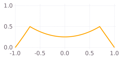
Figure 1. Numerical solution of problem (2.1) for $M=0.5$ and $q=1$.

Theorem 2.1 shows that a solution of problem (2.1) is given by a piecewise linear and parabolic function (see also the result of a numerical simulation in Figure 1). Notice that the high profile assumption $2M\geq q$ ensures that $u_{M;q}$ fits the interval $[0,M]$ and is therefore admissible for problem (2.1). The parabolic profile in the center has second derivative equal to $q$. A first understanding of this fact comes from the following straightforward first variation argument.

Proposition. Let $u$ be a solution to problem (2.1) and suppose that $u\in C^{2}(I)$ for some open interval $I\subset[-1,1]$. Moreover, suppose that $0<u<M$ in $I$. Then either $u^{\prime\prime}\equiv 0$ or $u^{\prime\prime}\equiv q$ in $I$.

Indeed, by $q$-concavity we have $u^{\prime\prime}\leq q$ in $I$. Suppose that $u^{\prime\prime}$ is not identically equal to $q$ in $I$, so that there exists an open interval $J\subset I$ such that $u^{\prime\prime}<q$ in $J$. Then, if $\varphi\in C^{\infty}_{c}(J)$ and $|t|$ is small enough, $u+t\varphi$ is still $q$-concave with $0<u+t\varphi<M$ (it is an admissible competitor). We have by dominated convergence

$$\frac{d}{dt}E(u+t\varphi) =-2\int_{J}\frac{\varphi^{\prime}(x)(u^{\prime}(x)+t\varphi^{\prime}(x))}{(1+(u^{\prime}(x)+t\varphi^{\prime}(x))^{2})^{2}}\,dx.$$

By minimality of $u$ we obtain that for any $\varphi\in C^{\infty}_{c}(J)$ there holds

$$-2\int_{J}\frac{\varphi^{\prime}u^{\prime}}{(1+(u^{\prime})^{2})^{2}}=2\int_{J}\frac{u^{\prime\prime}(1-(u^{\prime})^{2})}{(1+(u^{\prime})^{2})^{2}}\,\varphi=0,$$

so that we obtain the standard Euler-Lagrange equation for the Newton functional in one dimension

$$\frac{u^{\prime}}{(1+u^{\prime 2})^{2}}=\mathrm{const},$$

yielding that $u^{\prime\prime}\equiv 0$ in $J$ and then in $I$.

Radial two-dimensional case

In this case we let $\Omega=B_{R}(0)$ be the open ball in $\mathbb{R}^{2}$, with center $0$ and radius $R>0$, and we consider the class of $q$-concave radial functions. If we set $M>0$, $q\geq 0$ and

$$\mathcal{R}_{R;M;q}:=\left\{u\colon[0,R]\to[0,M]\left|r\mapsto u(r)-\frac{q}{2}r^{2}\text{ is nonincreasing and concave}\right.\right\},$$

then for every $u\in\mathcal{R}_{R;M;q}$ (which is the radial profile of a radial function that we still denote by $u$) the resistance functional is

$$D_{{B_{R}(0)}}(u)=\mathscr{D}_{R}(u):=\int\limits_{0}^{R}\dfrac{r\,dr}{1+u^{\prime}(r)^{2}}.$$

Therefore, given $M>0$, $R>0$ and $q\geq 0$, we have to solve the problem

(2.3) $$\min\left\{\mathscr{D}_{R}(u)\colon u\in\mathcal{R}_{R;M;q}\right\},$$

still with the high profile assumption $2M\geq qR^{2}$ and the single shock assumption $0\leq qR\leq 1$. Existence of minimizers is again standard, see the Appendix. Our second main result is the characterization of the solution to problem (2.3). It is given by a parabolic profile in $[0,a]$, and a strictly decreasing profile satisfying the radial two-dimensional Euler-Lagrange equation

$$\dfrac{-ru^{\prime}(r)}{(1+u^{\prime}(r)^{2})^{2}}=\mathrm{const}$$

in $(a,R]$. The optimal value of $a$ is uniquely determined in $(0,R)$. In order to write down the solution, which is a little less explicit, we need to introduce some notation.

We let $(-\infty,-1]\ni t\mapsto h(t):=-t(1+t^{2})^{-2}$. For $a\in(0,R)$, let $\varphi(a):=-\int_{a}^{R}h^{-1}(\tfrac{a}{4r})\,dr$ and

$$\gamma_{q}(a):=\sqrt{\dfrac{1}{2}\big{(}3a^{2}q^{2}+1+\sqrt{9a^{4}q^{4}+10a^{2}q^{2}+1}\big{)}},\quad\zeta_{q}(a):=-\int_{a}^{R}h^{-1}\left(\frac{ah(-\gamma_{q}(a))}{r}\right)\,dr.$$

Theorem 2.2.

Let $R>0$, $M>0$. Assume that $0\leq qR\leq 1$ and $2M\geq qR^{2}$. Then there exists a unique $a_{M}\in(0,R)$ such that $\varphi(a_{M})=M$, and there exists a unique $a_{*}\in[a_{M},R)$ such that $\zeta_{q}(a_{*})=M$. Moreover, there exists a unique solution to problem (2.3), given by

$$u(r):=\left\{\begin{array}[]{lcl}\dfrac{q}{2}(r^{2}-a_{*}^{2})+M&\text{if}&r\in[0,a_{*}]\\ &\\ \displaystyle-\int_{r}^{R}h^{-1}\left(\frac{a_{*}h(-\gamma_{q}(a_{*}))}{s}\right)\,ds&\text{if}&r\in(a_{*},R].\end{array}\right.$$

It is worth noticing that $\gamma_{0}(a)\equiv 1$, hence when $q=0$ we get $a_{*}=a_{M}$, and we recover the classical concave radial minimizer.

Numerical solutions to problem (2.3), in agreement with Theorem 2.2, are shown in Figure 2. We refer to Section 6 for numerical solutions obtained without radiality assumption.

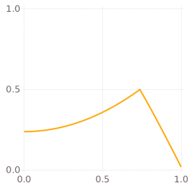
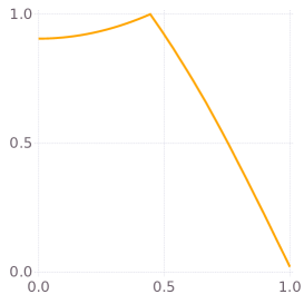
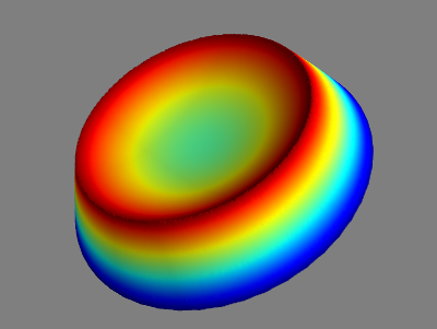
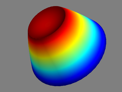
Figure 2. Numerical solutions of problem (2.3) for $M=0.5$ and $M=1$, both for $R=q=1$.

3. Some preliminary results

This section gathers some elementary results that will be useful in the sequel. We recall that, for $a<b$ and $q\geq 0$, $u:[a,b]\to\mathbb{R}$ is $q$-concave if the map $[a,b]\ni x\mapsto u(x)-\tfrac{q}{2}x^{2}$ is concave.

Definition 3.1 (Piecewise parabolic approximation).

Let $a<b$ and $q\geq 0$. Let $u$ be a $q$-concave continuous function on $[a,b]$. Let $w\colon[a,b]\to\mathbb{R}$ be defined by

$$w(y):=u(y)-\dfrac{q}{2}(y-a)(y-b).$$

For every $h\in\mathbb{N}$ and for every $j\in\left\{0,\ldots,h-1\right\}$ we consider intervals defined by $I_{j,h}:=\left[\alpha_{j,h},\beta_{j,h}\right)$ and $\alpha_{j,h}:=a+j\frac{b-a}{h}$, $\beta_{j,h}:=a+(j+1)\frac{b-a}{h}$. We let $w_{h}\colon[a,b]\to\mathbb{R}$ be given by

$$w_{h}(y):=\left\{\begin{array}[]{lcl}\sum\limits_{j=0}^{h-1}\left[w\left(\alpha_{j,h}\right)+\dfrac{h}{b-a}\left(w\left(\beta_{j,h}\right)-w\left(\alpha_{j,h}\right)\right)(y-\alpha_{j,h})\right]\mathbbm{1}_{I_{j}}(y)&\text{if}&y\in[a,b)\\ w(b)&\text{if}&y=b.\end{array}\right.$$

We define now the sequence of piecewise parabolic approximations $u_{h}\colon[a,b]\to\mathbb{R}$ as

$$u_{h}(y):=w_{h}(y)+\dfrac{q}{2}(y-a)(y-b),\qquad h\in\mathbb{N}.$$

Proposition 3.2.

Let $a<b$ and $q\geq 0$. Let $u$ be a $q$-concave continuous function on $[a,b]$. Let $(u_{h})_{h\in\mathbb{N}}$ be the sequence of piecewise parabolic approximations of $u$ given by Definition 3.1. Then $D_{(a,b)}(u_{h})\to D_{(a,b)}(u)$ as $h\to\infty$.

Proof.

We have $u_{h}\to u$ uniformly on $[a,b]$ as $h\to\infty$. For any differentiability point $x$ of $u$ which for every $h\in\mathbb{N}$ is not a grid node (that is, for a.e. $x\in(a,b)$), there holds $u^{\prime}_{h}(x)\to u^{\prime}(x)$. The result follows by dominated convergence. ∎

Remark 3.3.

It is clear that the approximation procedure of Definition 3.1 can be generalized to non uniform grids, still with $u_{h}$ equal to $u$ at grid nodes. Then, uniform convergence, a.e. convergence of derivatives and the result of Proposition 3.2 still hold as soon as the maximal size of the grid steps vanishes. In such case, it is possible to let an arbitrarily chosen point in $(a,b)$ be a grid node for any $h$. It is also possible to fix the value of the (right or left) derivative of the approximating sequence at some point. For instance, one may require $(u^{\prime}_{h})_{+}(x_{0})=u^{\prime}_{+}(x_{0})$ for any $h$ at some $x_{0}\in(a,b)$. Indeed, by the monotonicity of $w^{\prime}_{+}$, it is possible to find a sequence of intervals $[x_{h},x^{h})\ni x_{0}$, $h\in\mathbb{N}$, such that $x_{h}\uparrow x_{0}$ and $x^{h}\downarrow x_{0}$ monotonically as $h\to\infty$, and such that $(w(x^{h})-w(x_{h}))/(x^{h}-x_{h})=w^{\prime}_{+}(x_{0})$ for any $h$. Then, by choosing $x_{h},x^{h}$ to be subsequent grid nodes for the piecewise linear approximation $w_{h}$ of $w$, the requirement is fulfilled.

Proposition 3.4 (Parallelogram rule).

Let $\gamma\leq\delta$ and $c\geq 0$. Then

$$\int\limits_{\gamma}^{\delta}\dfrac{dx}{1+c(x-\gamma)^{2}}=\int\limits_{\gamma}^{\delta}\dfrac{dx}{1+c(x-\delta)^{2}}.$$

Proof.

The thesis follows by the change of variable $x\mapsto\gamma+\delta-x$. ∎

Proposition 3.5.

Let $a<b$ and $q\geq 0$. Let $u$ be a $q$-concave function on $[a,b]$ such that $u(a)=u(b)\geq u(x)$ for every $x\in[a,b].$ Then

$$\dfrac{q}{2}(x-b)\leq u^{\prime}_{+}(x)\leq u^{\prime}_{-}(x)\leq\dfrac{q}{2}(x-a)$$

for every $x\in(a,b).$

Proof.

Let $x\in(a,b)$ be fixed. Then, by $q$-concavity of $u$ on $[a,b]$, we have that both $u^{\prime}_{+}(x)$ and $u^{\prime}_{-}(x)$ exist and the following hold

(3.1) $$u(y)\leq u(x)+u^{\prime}_{+}(x)(y-x)+\dfrac{q}{2}(y-x)^{2}\text{ for every }y\in[x,b],$$

(3.2) $$u(z)\leq u(x)+u^{\prime}_{-}(x)(z-x)+\dfrac{q}{2}(z-x)^{2}\text{ for every }z\in[a,x].$$

Writing (3.1) for $y=b$ and (3.2) for $z=a$, taking into account that $u(a)=u(b)\geq u(x)$, we get

$$u^{\prime}_{+}(x)\geq\dfrac{q}{2}(x-b)\quad\text{ and }\quad u^{\prime}_{-}(x)\leq\dfrac{q}{2}(x-a).$$

Moreover, since $x\mapsto u(x)-\tfrac{q}{2}x^{2}$ is a concave function on $[a,b]$, then $u^{\prime}_{-}(x)\geq u_{+}^{\prime}(x)$ for every $x\in(a,b)$ thus concluding the proof. ∎

We conclude this preliminary section with the following computation.

Proposition 3.6.

Let $\lambda\geq 0$, $F_{\lambda}\colon\mathbb{R}^{3}\to\mathbb{R}$ be the function defined by

(3.3) $$F_{\lambda}(x,y,z):=\arctan x+\arctan y+\arctan z-\arctan\lambda+\arctan(\lambda-x)-\arctan(y+z)$$

and let

(3.4) $$\Delta_{\lambda}:=\left\{(x,y,z)\in\mathbb{R}^{3}\colon-y\leq x\leq\lambda,\,-\lambda\leq 2y\leq 0,\,x-\lambda\leq z\leq 0\right\}\subseteq\mathbb{R}^{3}.$$

Then

$$\min\limits_{\Delta_{\lambda}}F_{\lambda}=0.$$

The minimal value is attained if and only if one of the following three cases occurs:

$$\text{i) }\>x=\lambda,z=0,y\in\left[-\tfrac{\lambda}{2},0\right],\quad\text{ii) }\>x=-y,z=-y-\lambda,y\in\left[-\tfrac{\lambda}{2},0\right],\quad\text{iii) }\>x=y=0,z\in[-\lambda,0].$$

Proof.

If $\lambda=0$ the result is trivial. Let us assume that $\lambda>0$.

We first claim that if $(\overline{x},\overline{y},\overline{z})$ minimizes $F_{\lambda}$ on $\Delta_{\lambda}$, then $\overline{x}=-\overline{y}$ or $\overline{x}=\overline{z}+\lambda.$ Indeed, if $(\overline{x},\overline{y},\overline{z})$ is a minimum point for $F_{\lambda}$ on $\Delta_{\lambda}$ satisfying

(3.5) $$-\overline{y}<\overline{x}<\overline{z}+\lambda,$$

then it is seen from (3.4) that there exists $\delta>0$ such that $[\overline{x}-\delta,\overline{x}+\delta]\times\{\overline{y}\}\times\{\overline{z}\}\subseteq\Delta_{\lambda}$ and

$$0=\partial_{1}F_{\lambda}(\overline{x},\overline{y},\overline{z})=\dfrac{\lambda(\lambda-2\overline{x})}{\left(1+\overline{x}^{2}\right)\left(1+(\lambda-\overline{x})^{2}\right)},$$

that is $\overline{x}=\tfrac{\lambda}{2}$. Then, from (3.4) and(3.5) we have

$$-\dfrac{\lambda}{2}<\overline{y}\leq 0\text{ and }-\frac{\lambda}{2}<\overline{z}\leq 0.$$

If $\overline{x}=\frac{\lambda}{2}$, $-\tfrac{\lambda}{2}<\overline{y}<0\text{ and }-\frac{\lambda}{2}<\overline{z}<0$, then we see from (3.4) and (3.5) that the point $(\overline{x},\overline{y},\overline{z})$ is in the interior of $\Delta_{\lambda}$ and therefore

$$\partial_{2}F_{\lambda}\left(\overline{x},\overline{y},\overline{z}\right)=\partial_{3}F_{\lambda}\left(\overline{x},\overline{y},\overline{z}\right)=0,$$

but this is an absurd because the latter equalities hold true only if $\overline{y}=\overline{z}=0$. Then we are left to consider the case $\overline{x}=\frac{\lambda}{2}$, $\overline{y}=0$, $-\frac{\lambda}{2}<\overline{z}\leq 0$ and the case $\overline{x}=\frac{\lambda}{2}$, $-\tfrac{\lambda}{2}<\overline{y}\leq 0$, $\overline{z}=0$. However, in both cases we obtain

$$F_{\lambda}(\overline{x},\overline{y},\overline{z})=2\arctan\dfrac{\lambda}{2}-\arctan\lambda>0=F_{\lambda}(0,0,0)$$

and this contradicts the minimality of $(\overline{x},\overline{y},\overline{z})$, since $(0,0,0)\in\Delta_{\lambda}.$ The proof of the claim is done, that is, there holds $\overline{x}=\overline{z}+\lambda$ or $\overline{x}=-\overline{y}$.

In order to conclude it suffices to minimize the functions $\varphi_{\lambda},\psi_{\lambda}\colon\mathbb{R}^{2}\to\mathbb{R}$, defined by

$$\varphi_{\lambda}(y,z):=F(z+\lambda,y,z)=\arctan(z+\lambda)+\arctan y-\arctan\lambda-\arctan(y+z),$$

$$\psi_{\lambda}(y,z):=F(-y,y,z)=\arctan z-\arctan\lambda+\arctan(\lambda+y)-\arctan(y+z),$$

on the set

$$\Sigma_{\lambda}:=\left\{(y,z)\in\mathbb{R}^{2}\colon y\in\left[-\tfrac{\lambda}{2},0\right],z\in[-\lambda-y,0]\right\}.$$

It is easily seen than both $\varphi_{\lambda}$ and $\psi_{\lambda}$ have no critical points in the interior of ${\Sigma_{\lambda}}$. Let us check their behavior on the boundary of $\Sigma_{\lambda}$.

There holds

(3.6) $$\varphi_{\lambda}(y,0)=0=\varphi_{\lambda}(y,-y-\lambda)\quad\mbox{for every $y\in\left[-\tfrac{\lambda}{2},0\right]$}.$$

The restrictions of $\varphi_{\lambda}$ on the other two edges of the boundary of $\Sigma_{\lambda}$ are

$$\tilde{\varphi}_{\lambda}(z):=\varphi_{\lambda}\left(-\tfrac{\lambda}{2},z\right)=\arctan(z+\lambda)-\arctan\tfrac{\lambda}{2}-\arctan\lambda-\arctan\left(z-\tfrac{\lambda}{2}\right),\quad z\in\left[-\tfrac{\lambda}{2},0\right]$$

and

$$\overline{\varphi}_{\lambda}(z):=\varphi_{\lambda}(0,z)=\arctan(z+\lambda)-\arctan\lambda-\arctan z,\quad z\in[-\lambda,0].$$

Then we can see that $\tilde{\varphi}_{\lambda}$ is strictly increasing in $\left[-\tfrac{\lambda}{2},-\tfrac{\lambda}{4}\right]$ and strictly decreasing in $\left[-\tfrac{\lambda}{4},0\right]$ while $\overline{\varphi}_{\lambda}$ is strictly increasing in $[-\lambda,-\tfrac{\lambda}{2}]$ and strictly decreasing in $\left[-\tfrac{\lambda}{2},0\right]$. This yields $\tilde{\varphi}_{\lambda}\geq 0$ on $[-\frac{\lambda}{2},0]$ with equality only at $-\frac{\lambda}{2}$ and $0$, and $\overline{\varphi}_{\lambda}>0$ on $[-\lambda,0]$ with equality only at $-\lambda$ and $0$. Therefore, $\varphi_{\lambda}\geq 0$ on $\Sigma_{\lambda}$, the only equality cases being described by (3.6).

Similarly, $\psi_{\lambda}(0,z)=0$ for every $z\in[-\lambda,0]$ and $\psi_{\lambda}(y,-y-\lambda)=0$ for every $y\in\left[-\tfrac{\lambda}{2},0\right]$, and moreover $\psi_{\lambda}>0$ on the rest of the boundary of $\Sigma_{\lambda}$. Indeed, after setting

$$\tilde{\psi}_{\lambda}(z):=\psi_{\lambda}\left(-\tfrac{\lambda}{2},z\right)=\arctan z-\arctan\lambda+\arctan\tfrac{\lambda}{2}-\arctan\left(z-\tfrac{\lambda}{2}\right),\quad z\in\left[-\tfrac{\lambda}{2},0\right]$$

and

$$\overline{\psi}_{\lambda}(y):=\psi_{\lambda}(y,0)=-\arctan\lambda+\arctan(\lambda+y)-\arctan y,\quad y\in\left[-\tfrac{\lambda}{2},0\right]$$

it is easily seen that $\tilde{\psi}_{\lambda}$ is strictly increasing in $\left[-\tfrac{\lambda}{2},0\right]$ and $\overline{\psi}_{\lambda}$ is strictly decreasing on the same interval. The proof is concluded. ∎

4. The one-dimensional case

In the following we will make use of the notation

$$\wp_{a;b}^{K}(y):=\dfrac{q}{2}(y-a)(y-b)+K,\quad\text{ }y\in[a,b].$$

The proof of Theorem 2.1 is essentially based on the following Lemma 4.1 and Lemma 4.7. The first identifies the parabolic profile as optimal in the center. The latter identifies a linear profile on the side.

Lemma 4.1 (The center).

Let $a<b$, $q\geq 0$, and let $u$ be a $q$-concave function on $[a,b]$ such that $u(a)=u(b)\geq u(x)$ for every $x\in[a,b].$ Then

$$D_{(a,b)}(u)\geq D_{(a,b)}\left(\wp_{a;b}^{u(a)}\right)$$

and equality holds if and only if $u\equiv\wp_{a;b}^{u(a)}$.

Proof.

If $q=0$ the result is trivial. Assume therefore that $q>0$. Since $v_{h}(x):=u(x-h)$ satisfies $D_{(a,b)}(u)=D_{(a+h,b+h)}(v_{h})$ for any $h\in\mathbb{R}$ (translation invariance property), we may also assume without loss of generality that the reference interval is of the form $[-a,a]$, $a>0$.

Notice that $u$ is absolutely continuous in $[-a,a]$ and that $u(a)=u(-a)$ entails $\int_{-a}^{a}u^{\prime}(x)\,dx=0$, hence the set $\{x\in(-a,a):u^{\prime}_{+}(x)\leq qx\}$ is nonempty and we may define

(4.1) $$\zeta:=\inf\{x\in(-a,a)\colon u^{\prime}_{+}(x)\leq qx\}.$$

Then we have $\zeta\in[-a,a)$, and moreover we may assume without loss of generality that $\zeta\leq 0$ (indeed, if this is not the case we may consider $v(x):=u(-x)$, which still satisfies the assumptions, since it is clear that the corresponding value of $\zeta$ is in $[-a,0]$, and since $D_{-a}^{a}(v)=D_{-a}^{a}(u)$ obviously holds). Notice also that $\zeta\leq 0$ implies $u^{\prime}_{+}(0)\leq 0$, since $x\mapsto u^{\prime}_{+}(x)-qx$ is nonincreasing.

The proof will be achieved in some steps. We first prove that

(4.2) $$D_{(-a,a)}(u)\geq D_{(-a,a)}\left(\wp_{-a;a}^{u(a)}\right)$$

holds true for $q$-concave functions $u$, satisfying $u(a)=u(-a)\geq u(x)$ for any $x\in[-a,a]$, such that $[-a,a]\ni x\mapsto u(x)-\tfrac{q}{2}(x^{2}-a^{2})$ is piecewise linear. In such case $x\mapsto u^{\prime}(x)-qx$ is a nonincreasing piecewise constant function on $(-a,a)$. We will consider a general $u$ only in the last step.

Step 1. As previously observed, it is not restrictive to assume $\zeta\leq 0$. Let $A_{1}$ the (possibly empty) set defined by $A_{1}:=\{x\in(-a,\zeta)\colon u_{+}^{\prime}(x)>0\},$ and let $A_{2}=(-a,\zeta)\setminus A_{1}.$ Since $u^{\prime}$ is piecewise linear, $A_{1}$ is a finite disjoint union of open intervals $(c_{i},d_{i})$, $i=1,\ldots,k$, and

(4.3) $$\int\limits_{A_{1}}\dfrac{dx}{1+u^{\prime}(x)^{2}} \geq\sum\limits_{i=1}^{k}\int\limits_{c_{i}}^{d_{i}}\dfrac{dx}{1+q^{2}(x-c_{i})^{2}}$$

$$=\sum\limits_{i=1}^{k}\int\limits_{c_{i}}^{d_{i}}\dfrac{dx}{1+q^{2}(x-d_{i})^{2}}\geq\sum\limits_{i=1}^{k}\int\limits_{c_{i}}^{d_{i}}\dfrac{dx}{1+q^{2}x^{2}}=\int\limits_{A_{1}}\dfrac{dx}{1+q^{2}x^{2}}.$$

Here, the first inequality holds true since $x\mapsto u_{+}^{\prime}(x)-qx$ (equal to $u^{\prime}(x)-qx$ a.e. on $(-a,a)$) is not increasing and since $u^{\prime}_{+}(c_{i})=0$, so that on $(c_{i},d_{i})$ we have $0<u^{\prime}_{+}(x)\leq q(x-c_{i})$. The first equality follows by Proposition 3.4 and the last inequality is satisfied since we have $d_{i}\leq 0$ and then $0<q(d_{i}-x)\leq-qx$ on $(c_{i},d_{i})$, for every $i=1,\ldots,k$. On the other hand, it is clear that we have $0\geq u^{\prime}_{+}(x)\geq qx$ on $A_{2}$ and together with (4.3) this gives

(4.4) $$D_{(-a,\zeta)}(u)=\int_{A_{1}\cup A_{2}}\frac{dx}{1+u^{\prime}(x)^{2}}\geq\int_{-a}^{\zeta}\frac{dx}{1+q^{2}x^{2}}.$$

In a similar way, since $u$ is $q$-concave on $[-a,a]$ and $\zeta\in[-a,0]$, we have that $0\geq qx\geq u^{\prime}_{+}(x)\geq u^{\prime}_{+}(0)+qx$ for every $x\in(\zeta,0)$. As $u^{\prime}=u^{\prime}_{+}$ a.e. on $(-a,a)$, we get

(4.5) $$D_{(\zeta,0)}(u) \geq\int\limits_{\zeta}^{0}\dfrac{dx}{1+(u^{\prime}_{+}(0)+qx)^{2}}=\dfrac{1}{q}\arctan(u^{\prime}_{+}(0))-\dfrac{1}{q}\arctan(u^{\prime}_{+}(0)+q\zeta)$$

$$=\int\limits_{\zeta}^{0}\dfrac{dx}{1+q^{2}x^{2}}+\dfrac{1}{q}\arctan(u^{\prime}_{+}(0))-\dfrac{1}{q}\arctan(u^{\prime}_{+}(0)+q\zeta)+\dfrac{1}{q}\arctan(q\zeta).$$

Step 2. Let us now define

(4.6) $$\sigma: =\min\{x\in[0,a)\colon u^{\prime}_{+}(x)=0\},$$

$$S: =\{x\in(0,a)\colon u^{\prime}_{-}(x)=u^{\prime}_{+}(x)=0\}\cup\{x\in(0,a)\colon u^{\prime}_{+}(x)<0<u^{\prime}_{-}(x)\}.$$

By Proposition 3.5, we have $\tfrac{q}{2}(x-a)\leq u^{\prime}(x)\leq\tfrac{q}{2}(x+a)$ at each point where $u^{\prime}$ exists. Since $u^{\prime}(x)-qx$ is piecewise constant, it follows that $-qx>u^{\prime}(x)-qx\geq 0$ on a right neighbor of $-a$ and $-qx<u^{\prime}(x)-qx\leq 0$ on a left neighbor of $a$. Moreover $u^{\prime}_{+}(0)\leq 0$ follows from $\zeta\leq 0$. Therefore, $\sigma$ is well defined. We have $0<\sigma<a$ if $u^{\prime}_{+}(0)<0$ (then $u^{\prime}_{+}<0$ on $(0,\sigma)$) and $\sigma=0$ otherwise. In any case $u^{\prime}_{+}(\sigma)=0$. On the other hand, $u^{\prime}$ is piecewise linear, therefore $S$ is a (possibly empty) finite set, and sign change of $u^{\prime}_{+}$ on $(0,a)$ occurs exactly at $\sigma$ if $\sigma>0$, and on $S\setminus\{\sigma\}$, if nonempty. In case $S\setminus\{\sigma\}$ is nonempty, we denote its elements by $0<\xi_{1}<\xi_{2}<\ldots<\xi_{h}$, and $h$ is even (this comes from the fact that $u^{\prime}>0$ in a left neighborhood of $a$). We also let $\xi_{h+1}=a$. In each of the intervals $(\xi_{i},\xi_{i+1})$, $i=1,\ldots,h$, there holds either $u^{\prime}_{+}\geq 0$ or $u^{\prime}_{+}\leq 0$. Moreover we have that

(4.7) $$D_{(\xi_{i},\xi_{i+1})}(u)\geq\int\limits_{\xi_{i}}^{\xi_{i+1}}\dfrac{dx}{1+q^{2}(x-\xi_{i})^{2}}$$

for every $i=1,\ldots,h$. Indeed, (4.7) is obvious if $u^{\prime}_{+}\geq 0$ on $(\xi_{i},\xi_{i+1})$, i.e., $u^{\prime}\geq 0$ a.e. on $(\xi_{i},\xi_{i+1})$. Else if $u^{\prime}\leq 0$ a.e. on $(\xi_{i},\ \xi_{i+1})$, the $q$-concavity inequality $0\geq u^{\prime}_{+}(x)\geq q(x-\xi_{i+1})$ and Proposition 3.4 yield

$$D_{(\xi_{i},\xi_{i+1})}(u)\geq\int\limits_{\xi_{i}}^{\xi_{i+1}}\dfrac{dx}{1+q^{2}(x-\xi_{i+1})^{2}}=\int\limits_{\xi_{i}}^{\xi_{i+1}}\dfrac{dx}{1+q^{2}(x-\xi_{i})^{2}}.$$

If instead $S\setminus\{\sigma\}$ is empty we just have $h=0$ and $\xi_{1}=a$. Similarly, $q$-concavity implies $0\leq u^{\prime}_{+}(x)\leq q(x-\sigma)$ on $(\sigma,\xi_{1})$, and in case $\sigma>0$ it gives $q(x-\sigma)\leq u^{\prime}_{+}(x)\leq 0$ on $(0,\sigma)$. Then the usual change of variables of Proposition 3.4 entails

(4.8) $$D_{(0,\sigma)}(u)\geq\int\limits_{0}^{\sigma}\dfrac{dx}{1+q^{2}x^{2}},\qquad D_{(\sigma,\xi_{1})}(u)\geq\int\limits_{\sigma}^{\xi_{1}}\dfrac{dx}{1+q^{2}(x-\sigma)^{2}}.$$

In general, from (4.7) and (4.8) we have

$$D_{(0,a)}(u) =D_{(0,\sigma)}(u)+D_{(\sigma,{\xi_{1}})}(u)+\sum_{i=1}^{h}D_{(\xi_{i},\xi_{i+1})}(u)$$

$$\geq\int\limits_{0}^{\sigma}\dfrac{dx}{1+q^{2}x^{2}}+\int\limits_{\sigma}^{\xi_{1}}\dfrac{dx}{1+q^{2}(x-\sigma)^{2}}+\sum\limits_{i=1}^{h}\int\limits_{\xi_{i}}^{\xi_{i+1}}\dfrac{dx}{1+q^{2}(x-\xi_{i})^{2}}$$

$$=\int\limits_{0}^{\sigma}\dfrac{dx}{1+q^{2}x^{2}}+\dfrac{1}{q}\arctan(q\xi_{1}-q\sigma)+\sum_{i=1}^{h}\dfrac{1}{q}\arctan(q\xi_{i+1}-q\xi_{i}).$$

The sub-additivity of $\arctan$ in $\mathbb{R}_{+}$ then implies

(4.9) $$D_{(0,a)}(u) \geq\int\limits_{0}^{\sigma}\dfrac{dx}{1+q^{2}x^{2}}+\dfrac{1}{q}\arctan(qa-q\sigma)$$

$$=\int\limits_{0}^{a}\dfrac{dx}{1+q^{2}x^{2}}+\dfrac{1}{q}\arctan(qa-q\sigma)-\dfrac{1}{q}\arctan(qa)+\dfrac{1}{q}\arctan(q\sigma).$$

Step 3. Adding together (4.4), (4.5) and (4.9) we get

(4.10) $$D_{(-a,a)}(u)\geq\int\limits_{-a}^{a}\dfrac{dx}{1+q^{2}x^{2}}+\dfrac{1}{q}F_{qa}(q\sigma,u^{\prime}_{+}(0),q\zeta)$$

where $F_{qa}$ is the function defined in (3.3) with $\lambda=qa>0$, so that in order to conclude it is enough to show that

(4.11) $$(q\sigma,u^{\prime}_{+}(0),q\zeta)\in\Delta_{qa},$$

being $\Delta_{qa}$ the set defined in (3.4) with $\lambda=qa$, and then apply Proposition 3.6.

We already observed that $q\sigma\leq qa$, $u^{\prime}_{+}(0)\leq 0$ and $q\zeta\leq 0$. Moreover, $q$-concavity and $u^{\prime}_{+}(\sigma)=0$ yield $u^{\prime}_{+}(0)\geq u^{\prime}_{+}(\sigma)-q\sigma=-q\sigma$. Since $u(-a)=u(a)\geq u(x)$ for every $x\in[-a,a]$, by applying Proposition 3.5 we obtain that $2u^{\prime}_{+}(0)\geq-qa.$ At last we claim that $q\sigma-qa\leq q\zeta.$ Indeed we have $\int_{o}^{\sigma}u^{\prime}(x)dx\leq 0$ and $u^{\prime}(x)\leq q(x-\sigma)$ a.e. on $(\sigma,a)$, whereas $u(a)=u(-a)\geq u(\zeta)$ by assumption, thus

$$0 =\int\limits_{-a}^{a}u^{\prime}(t)\,dt=\int\limits_{-a}^{\zeta}u^{\prime}(t)\,dt+\int\limits_{\zeta}^{a}u^{\prime}(t)\,dt=u(\zeta)-u(a)+\int\limits_{\zeta}^{a}u^{\prime}(t)\,dt\leq\int\limits_{\zeta}^{a}u^{\prime}(t)\,dt$$

$$=\int\limits_{\zeta}^{0}u^{\prime}(t)\,dt+\int\limits_{0}^{\sigma}u^{\prime}(t)\,dt+\int\limits_{\sigma}^{a}u^{\prime}(t)\,dt\leq\int\limits_{\zeta}^{0}qt\,dt+\int\limits_{\sigma}^{a}q(t-\sigma)\,dt=\dfrac{1}{2}(a-\sigma-\zeta)(qa-q\sigma+q\zeta),$$

but $a-\sigma\geq 0$ and $\zeta\leq 0$ then the claim is proved, and (4.11) is shown, so that (4.10) and Proposition 3.6 allow to conclude that

$$D_{(-a,a)}(u)\geq\int\limits_{-a}^{a}\dfrac{dx}{1+q^{2}x^{2}}=D_{(-a,a)}\left(\wp_{-a;a}^{u(a)}\right),$$

in case $x\mapsto u^{\prime}(x)-qx$ is piecewise constant.

Step 4. In order to treat a general $q$-concave function $u$, satisfying $u(-a)=u(a)\geq u(x)$ for any $x\in[-a,a]$, we approximate it by means of the sequence $u_{h}$ from Definition 3.1. Then, (4.2) applies to $u_{h}$ for each $h$, as just shown. Invoking Proposition 3.2, we find (4.2) for $u$.

We are left to prove that the only equality case in (4.2) is $u=\wp_{-a;a}^{u(a)}$, i.e., $u^{\prime}(x)=qx$ in $(-a,a)$. This is done by revisiting the previous steps and by taking some care in the choice of the approximating sequence $u_{h}$. Assume that $u$ satisfies (4.2) with equality. As usual, we may assume that the number $\zeta$ defined by (4.1) is nonpositive, then $u^{\prime}_{+}(0)\leq 0$. If $\zeta=-a$, then $\int_{-a}^{a}u^{\prime}=0$ readily implies $u^{\prime}=qx$ on $(-a,a)$. Therefore, we assume that $\zeta>-a$ as well, and we aim at reaching a contradiction.

We first claim that $u^{\prime}_{+}\leq 0$ in the whole $(0,a)$ yields contradiction: indeed, it would give, by taking into account that $u(x)\leq u(-a)$ in $[-a,a]$ and that $u^{\prime}\leq 0$ a.e. on $(\zeta,0)$,

$$0=\int\limits_{-a}^{a}u^{\prime}(x)\,dx\leq\int\limits_{\zeta}^{a}u^{\prime}(x)\,dx=\int\limits_{\zeta}^{0}u^{\prime}(x)\,dx+\int\limits_{0}^{a}u^{\prime}(x)\,dx\leq\int\limits_{\zeta}^{0}qx\,dx\leq-\dfrac{q}{2}\zeta^{2},$$

that is, $\zeta=0$. But $\zeta=0$ implies $D_{(-a,0)}(u)\geq D_{(-a,0)}\left(\wp_{-a;a}^{u(a)}\right)$: this follows from Step 1, see (4.3) and (4.4), where in this case the set $A_{1}$ is a possibly infinite but countable union of disjoint open intervals (because $A_{1}$ is open, since $u^{\prime}_{+}$ is lower semicontinous). On the other hand, Proposition 3.5 implies $u^{\prime}(x)\geq\tfrac{q}{2}(x-a)$ a.e. on $(0,a)$, then $u^{\prime}\leq 0$ gives $u^{\prime}(x)^{2}\leq\tfrac{q^{2}}{4}(x-a)^{2}$ and Proposition 3.4 yields

$$D_{(0,a)}(u)=\int_{0}^{a}\frac{dx}{1+u^{\prime}(x)^{2}}\geq\int_{0}^{a}\frac{dx}{1+\tfrac{q^{2}}{4}(x-a)^{2}}=\int_{0}^{a}\frac{dx}{1+\tfrac{q^{2}}{4}x^{2}}>D_{(0,a)}\left(\wp_{-a;a}^{u(a)}\right),$$

that is, summing up, $D_{(-a,a)}(u)>D_{(-a,a)}(\tilde{u})$, a contradiction. The claim is proved and thus we assume from now that $u^{\prime}_{+}>0$ at some point in $(0,a)$, which implies, by $q$-concavity of $u$ and right continuity of $u^{\prime}_{+}$, that $\sigma$ from (4.6) is well defined for $u$, with $u^{\prime}_{+}(\sigma)=0$ and $-a<\zeta\leq 0\leq\sigma<a$.

We approximate $u$ with a sequence of $q$-concave piecewise parabolic functions $u_{h}$, constructed by means of Remark 3.3, such that $u_{h}(\pm a)=u(\pm a)$, $(u_{h})^{\prime}\to u^{\prime}$ a.e. on $(-a,a)$ and

(4.12) $$(u_{h})^{\prime}_{{+}}(\sigma)=u^{\prime}_{+}(\sigma),\quad(u_{h})^{\prime}_{{+}}(\zeta)=u^{\prime}_{+}(\zeta),\quad(u_{h})^{\prime}_{{+}}(0)=u^{\prime}_{+}(0),\quad\forall h\in\mathbb{N}.$$

We let $\zeta_{h}:=\inf\{x\in(-a,a)\colon(u_{h})^{\prime}_{+}(x)\leq qx\}$. By definition of $\zeta_{h}$ and $\zeta$ and by (4.12), we see that $\zeta_{h}\leq\zeta$ and that $\zeta_{h}\to\zeta$ as $h\to\infty$. We let $\sigma_{h}:=\min\{x\in[0,a)\colon(u_{h})^{\prime}_{+}(x)=0\}$, then (4.12) implies $\sigma_{h}\leq\sigma$. Notice that if $u^{\prime}_{+}(0)=0$, then $\sigma=0$ so that $\sigma_{h}=0$ for any $h$. Else if $(u_{h})^{\prime}_{+}(0)=u^{\prime}_{+}(0)<0$ we have by $q$-concavity $(u_{h})^{\prime}_{+}(x)\leq qx+u^{\prime}_{+}(0)$ on $[0,a)$, implying $q\sigma_{h}\geq-{(u_{h})^{\prime}_{+}(0)}=-u^{\prime}_{+}(0)$. Therefore $\sigma_{h}\in\left[-{u^{\prime}_{+}(0)}/{q},\sigma\right]$, and we may assume, up to passing on a not relabeled subsequence, that $\sigma_{h}\to\bar{\sigma}\in\left[-{u^{\prime}_{+}(0)}/{q},\sigma\right]$ as $h\to\infty$.

We apply the previous steps obtaining 4.10 for $u_{h}$, and passing to the limit with the a.e. convergence of $u^{\prime}_{h}$ to $u^{\prime}$ and with the continuity of function $F_{qa}$ we get

$$D_{(-a,a)}(u)\geq\int\limits_{-a}^{a}\dfrac{dx}{1+q^{2}x^{2}}+\dfrac{1}{q}F_{qa}(q\bar{\sigma},u^{\prime}_{+}(0),q\zeta).$$

If $F_{qa}(q\bar{\sigma},u^{\prime}_{+}(0),q\zeta)>0$ we contradict the fact that $u$ satisfies (4.2) with equality. By taking into account that $\bar{\sigma}\leq\sigma<a$, Proposition 3.6 shows that $F_{qa}(q\bar{\sigma},u^{\prime}_{+}(0),q\zeta)=0$ if and only if one of the following two cases occurs

$${\rm i)}\;0<u^{\prime}_{+}(0)=-q\bar{\sigma},\ \ \zeta=\bar{\sigma}-a,\qquad{\rm ii)}\;\bar{\sigma}=0=u^{\prime}_{+}(0).$$

If i) were true then $u^{\prime}_{+}(x)\leq qx+u^{\prime}_{+}(0)=q(x-\zeta-a)$ for every $x\in(0,a)$, hence by taking into account that $u(\zeta)\leq u(-a)$ we would get

$$0=\int_{-a}^{a}u^{\prime}(x)\,dx\leq\int_{\zeta}^{0}qx\,dx+\int_{0}^{a}q(x-\zeta-a)\,dx=-\dfrac{q}{2}(\zeta+a)^{2}$$

that is $\zeta=-a$, a contradiction.

Eventually if ii) occurs then we are in the case $\sigma_{h}=\sigma=0$. In this case it is clear that $u_{+}^{\prime}(x)-qx$, which is monotone, is identically $0$ on $(\zeta,0)$, and moreover we immediately get

(4.13) $$D_{(-a,0)}\left(\wp_{-a;a}^{u(a)}\right)\leq D_{(-a,0)}(u),$$

since equality holds on $(\zeta,0)$ where $u^{\prime}(x)\equiv qx$, and since we apply Step 1 on $(-a,\zeta)$, recalling as before that in general the set $A_{1}$ therein is a countable union of disjoint open intervals.

If $0\leq u^{\prime}_{+}(x)\leq qx$ in $(0,a)$, either $u^{\prime}=qx$ a.e. in $(0,a)$, thus in $(\zeta,a)$, and then we easily see from the null mean property of $u^{\prime}$ that $\zeta=-a$ (a contradiction), or $u^{\prime}=qx$ does not hold a.e. in $(0,a)$ and we readily conclude that $D_{(0,a)}\left(\wp_{-a;a}^{u(a)}\right)<D_{(0,a)}(u)$, which, combined with (4.13), yields that (4.2) does not hold with equality, a contradiction.

Else if $u^{\prime}_{+}<0$ at some point $c\in(0,a)$, since we are also excluding $u^{\prime}_{+}\leq 0$ on the whole $(0,a)$, we also fix a point $d\in(0,a)$ such that $u^{\prime}_{+}(d)>0$. In this case, we assume that the above approximating sequence $u_{h}$ satisfies a further restriction, still by means of Remark 3.3: we let $(u_{h})^{\prime}_{{+}}(c)=u^{\prime}_{+}(c)$ and $(u_{h})^{\prime}_{{+}}(d)=u^{\prime}_{+}(d)$ for any $h\in\mathbb{N}$. Therefore, after defining

$$S_{h}:=\{x\in(0,a)\colon(u_{h})^{\prime}_{-}(x)=(u_{h})^{\prime}_{+}(x)=0\}\cup\{x\in(0,a)\colon(u_{h})^{\prime}_{+}(x)<0<(u_{h})^{\prime}_{-}(x)\},$$

it is clear that for any $h\in\mathbb{N}$ there is an element $\bar{x}_{h}$ in the set $S_{h}\cap[c\wedge d,c\vee d]$. Indeed, $u_{h}^{\prime}$ has to change sign at least once on $[c\wedge d,c\vee d]$. Now we can reason as in Step 2. Fix $h\in\mathbb{N}$. Let $0=\xi_{0}<\xi_{1}<\ldots<\xi_{n}=\bar{x}_{h}$ and $\bar{x}_{h}=\xi_{n+1}\ldots<\xi_{n+m-1}$ denote the finitely many points of $S_{h}$, and let $\xi_{n+m}=a$ ($S_{h}$ contains at least $\bar{x}_{h}$). Since (4.7) holds for $u_{h}$ in any of the intervals $(\xi_{i},\xi_{i+1})$, where $u^{\prime}_{h}$ does not change sign, we get

$$D_{(0,a)}(u_{h}) \geq\sum_{i=0}^{n+m-1}\int_{\xi_{i}}^{\xi_{i+1}}\frac{dx}{1+q^{2}(x-\xi_{i})^{2}}=\sum_{i=0}^{n+m-1}\tfrac{1}{q}\arctan{(q(\xi_{i+1}-\xi_{i}))}$$

$$\geq\frac{1}{q}\arctan(q\bar{x}_{h})+\frac{1}{q}\arctan(q(a-\bar{x}_{h}))$$

where we have split the sum and used the sub-additivity of arctan. By passing to the limit with Proposition 3.2 and Remark 3.3 as $h\to\infty$ (possibly on a subsequence, such that $\bar{x}_{h}$ converge to some $\bar{x}\in[c\wedge d,c\vee d]$), and also using (4.13), we get

$$D_{(-a,a)}(u)\geq\int_{-a}^{0}\frac{dx}{1+q^{2}x^{2}}+\frac{1}{q}\arctan(q\bar{x})+\frac{1}{q}\arctan(q(a-\bar{x}))>\int_{-a}^{0}\frac{dx}{1+q^{2}x^{2}}+\frac{1}{q}\arctan(qa),$$

since $0<\bar{x}<a$. The right hand side is exactly $D_{(-a,a)}\left(\wp_{-a;a}^{u(a)}\right)$, this is a contradiction. ∎

Proposition 4.2 (concave rearrangement).

Let $a<b$ and let $u$ be a nonincreasing absolutely continuous function on $[a,b]$. Then there exists a nonincreasing concave function $u^{\ast}\colon[a,b]\to[u(b),u(a)]$ such that $D_{(a,b)}(u)=D_{(a,b)}(u^{\ast}).$

Proof.

Let $\left(u_{h}\right)_{h\in\mathbb{N}}$ denote a sequence of continuos, piecewise affine, nonincreasing approximating functions, constructed on a equispaced grid of step $(b-a)/h$ on the interval $[a,b]$, and coinciding with $u$ at the nodes of the grid. At any differentiability point $x$ of $u$ in $(a,b)$ which for any $h$ is not a grid node (that is, for a.e. $x$ in $(a,b)$), there holds $u_{h}^{\prime}(x)\to u^{\prime}(x)$ as $h\to\infty$.

For every $h\in\mathbb{N}$ let us exchange the position of each segment of the graph of $u_{h}$ in such a way that the slopes get ordered in a nonincreasing way. If $s_{j,h}$ denotes the slope of the piecewise affine function $u_{h}$ on the interval $[a+(b-a)(j-1)/h,a+(b-a)j/h]$, $j=1,\ldots,h$, we denote by $s^{*}_{1,h},\ldots,s^{*}_{h,h}$ a permutation of the slopes such that $s^{*}_{1,h}\geq s^{*}_{2,h}\geq\ldots\geq s^{*}_{h,h}$. We define $u_{h}^{*}$ as the unique continuous, piecewise affine function such that the slope of $u_{h}^{*}$ is $s^{*}_{j,h}$ on the interval $[a+(b-a)(j-1)/h,a+(b-a)j/h]$, $j=1,\ldots,h$, and such that $u_{h}^{*}(a)=u_{h}(a)=u(a)$, $u_{h}^{*}(b)=u_{h}(b)=u(b)$. It is clear that $D_{(a,b)}(u_{h}^{*})=D_{(a,b)}(u_{h})$ for every $h\in\mathbb{N}$.

Notice that $(u_{h}^{*})_{h\in\mathbb{N}}$ is a family of concave, uniformly bounded functions on $[a,b]$. By Lemma 7.5 in the Appendix, the family $(u_{h}^{*})_{h\in\mathbb{N}}$ has a concave decreasing limit point $u^{*}:[a,b]\to[u(b),u(a)]$ in the strong $W^{1,1}_{loc}((a,b))$ topology (it is extended by continuity to the closed interval). This entails uniform convergence on compact subsets of $(a,b)$ and $a.e.$ convergence of derivatives (up to extracting a subsequence), allowing to pass to the limit with dominated convergence and to get

$$D_{(a,b)}(u^{*})=\lim_{h\to\infty}D_{(a,b)}(u_{h}^{*})=\lim_{h\to\infty}D_{(a,b)}(u_{h})=D_{(a,b)}(u).$$

Hence, $u^{*}$ is the desired concave rearrangement. ∎

Remark 4.3.

In the same assumptions of Proposition 4.2 and with the same notation, if $c<0$ exists such that the set of differentiability points of $u$ with $u^{\prime}>c$ has positive measure, the same property holds for $u^{*}$ as well. Indeed, in such case there exists $\varepsilon>0$ such that the set $B$ where $u^{\prime}>c+\varepsilon$ has positive measure as well. Since $u_{h}^{\prime}$ converge to $u^{\prime}$ a.e. on $B$, by Egorov theorem there is a positive measure subset $B^{*}$ of $B$ such that $u^{\prime}_{h}\to u^{\prime}$ uniformly on $B^{*}$. Then there exists $h_{0}>0$ such that, for any $h>h_{0}$ and any $x\in B^{*}$, there holds $u_{h}^{\prime}(x)>c+\varepsilon/2$. For any $h>h_{0}$, after rearranging, since $u_{h}^{*}$ are concave, we have $(u_{h}^{*})^{\prime}>c+\varepsilon/2$ a.e. on an interval $(a,\xi)$ with length equal to the measure of $B^{*}$. Since $(u_{h}^{*})^{\prime}\to(u^{*})^{\prime}$ a.e. on $(a,b)$, we conclude that $(u^{*})^{\prime}\geq c+\varepsilon/2>c$ a.e. on $(a,\xi)$.

For the proof of Lemma 4.7 below, we will need a general result about the resistance functional, holding also in higher dimension. It is the property $|\nabla u|\notin(0,1)$, a proof of which is given in [BFK2, Theorem 2.3]. In dimension one we provide a simpler proof with the following

Proposition 4.4.

Let $a<b$ and let $u$ be a concave, nonincreasing, continuous function on $[a,b]$, such that $u(a)>u(b)$. Then there exists $c\in[a,b)$ such that $u(a)-u(b)\geq b-c$ and

$$D_{(a,b)}(u)\geq D_{(a,b)}(u_{a;b}^{c}),$$

where $u_{a;b}^{c}\colon[a,b]\to\mathbb{R}$ is defined by

(4.14) $$u^{c}_{a;b}(y):=\left\{\begin{array}[]{lcl}u(a)&\text{if}&y\in[a,c]\\ \\ \dfrac{y-b}{c-b}\left(u(a)-u(b)\right)+u(b)&\text{if}&y\in(c,b].\end{array}\right.$$

Proof.

Since $u$ is concave, then the set $A_{u}:=\{x\in(a,b)\colon u^{\prime}_{+}(x)\geq-1\}$ is connected, and we define

$$c^{\ast}:=\left\{\begin{array}[]{lll}\sup{A_{u}}&\text{if}&A_{u}\neq\varnothing\\ a&\text{if}&A_{u}=\varnothing\end{array}\right.$$

and $u_{c^{\ast}}\colon[a,b]\to\mathbb{R}$ as follows:

$$u_{c^{\ast}}(x):=\left\{\begin{array}[]{lll}u(a)&\text{if}&x\in[a,c^{\ast}+u(c^{\ast})-u(a)]\\ -x+c^{\ast}+u(c^{\ast})&\text{if}&x\in[c^{\ast}+u(c^{\ast})-u(a),c^{\ast}]\\ u(x)&\text{if}&x\in[c^{\ast},b].\end{array}\right.$$

Since $\tfrac{1}{1+t^{2}}\geq 1+\tfrac{t}{2}$ for every $t\leq 0$, we have

$$D_{(a,c^{\ast})}(u)\geq\int\limits_{a}^{c^{\ast}}\left(1+\dfrac{u^{\prime}(x)}{2}\right)dx=c^{\ast}-a+\dfrac{1}{2}(u(c^{\ast})-u(a))=D_{(a,c^{\ast})}(u_{c^{\ast}})$$

where the last equality follows by a simple calculation. Then $D_{(a,b)}(u)\geq D_{(a,b)}(u_{c^{\ast}})$.

Let now $c:=c^{\ast}+u(c^{\ast})-u(a)$. We claim that $D_{(a,b)}(u_{c^{\ast}})\geq D_{(a,b)}(u^{c}_{a;b})$. To see this, it is enough to prove that $D_{(c,b)}(u_{c^{\ast}})\geq D_{(c,b)}(u^{c}_{a;b})$. This immediately follows by Jensen inequality, since the function $f\colon(-\infty,-1]\to\mathbb{R}$ defined by $f(t)=\tfrac{1}{1+t^{2}}$ is convex and $u_{c^{\ast}}^{\prime}\leq-1$ a.e. in $(c,b)$. ∎

Corollary 4.5.

Let $a<b$ and let $u$ be a nonincreasing absolutely continuous function on $[a,b]$, such that $u(a)>u(b)$. Then there exists $c\in[a,b)$ such that $u(a)-u(b)\geq b-c$ and

$$D_{(a,b)}(u)\geq D_{(a,b)}(u^{c}_{a;b}),$$

where $u^{c}_{a;b}\colon[a,b]\to\mathbb{R}$ is the function defined in (4.14).

Proof.

We apply Proposition 4.2 to $u$, obtaining a nonincreasing concave function $u^{\ast}\colon[a,b]\to[u(b),u(a)]$ such that $D_{(a,b)}(u)=D_{(a,b)}(u^{\ast})$. Since $u(a)>u(b)$, then $u^{*}$ is non constant. We apply Proposition 4.4 to $u^{*}$, obtaining $c\in[a,b)$ and $(u^{\ast})^{c}_{a;b}$, defined by means of (4.14), such that $u(a)-u(b)\geq u^{*}(a)-u^{*}(b)\geq b-c$ and $D_{(a,b)}(u^{*})\geq D_{(a,b)}((u^{*})^{c}_{a;b})$. But then we easily see that $D_{(a,b)}((u^{*})^{c}_{a;b})\geq D_{(a,b)}(u^{c}_{a;b})$ and we conclude. ∎

Remark 4.6.

Notice that the condition $u(a)-u(b)\geq b-c$ on $c$ indicates that the straight line corresponding to the restriction of $u_{a;b}^{c}$ on $[c,b]$ has slope smaller than or equal to $-1$.

Lemma 4.7 (The side).

Let $a<b$ and $q\geq 0$. Let $u$ be a $q$-concave continuous function on $[a,b]$ such that $u(y)\leq u(a)$ for every $y\in[a,b]$ and $u(b)<u(a)$. Then there exists $\gamma\in[a,b)$ such that $u(a)-u(b)\geq b-\gamma$ and

$$D_{(a,b)}(u)\geq D_{(a,b)}(w_{a,\gamma,b}),$$

where $w_{a,\gamma,b}\colon[a,b]\to\mathbb{R}$ is defined by

(4.15) $$w_{a,\gamma,b}(y):=\left\{\begin{array}[]{lcl}\wp_{a;\gamma}^{u(a)}(y)&\text{if}&y\in[a,\gamma)\\ \\ \dfrac{y-b}{\gamma-b}\left(u(a)-u(b)\right)+u(b)&\text{if}&y\in[\gamma,b].\end{array}\right.$$

The result holds with $\gamma\in(a,b)$ if $u$ is not strictly decreasing on $[a,b]$.

Proof.

If $q=0$ we just apply Proposition 4.4, obtaining the concave function $u_{a;b}^{c}$, defined in (4.14), with $c\in[a,b)$, such that $D_{(a,b)}(u)\geq D_{(a,b)}(u_{a;b}^{c})$. Then we just let $\gamma=c$ and observe that in case $q=0$ we have $u_{a;b}^{\gamma}=w_{a,\gamma,b}$. If $u$ is not strictly decreasing and it is concave, then it has a flat part in a neighborhood of $a$ and we can take $c>a$. This is done by fixing $\tilde{a}>a$ such that $u(\tilde{a})=u(a)$ and by applying Proposition 4.4 on $[\tilde{a},b]$. From here on, we let $q>0$.

As did in the proof of Lemma 4.1, we prove the result first for $q$-concave functions $u$ that satisfy the assumptions (i.e. $u(x)\leq u(a)$ on $[a,b]$, $u(a)>u(b)$) and are moreover such that $[a,b]\ni x\mapsto u(x)-\tfrac{q}{2}(x-a)(x-b)$ is piecewise linear. This means that $u$ is piecewise parabolic on $[a,b]$, the second derivative of $u$ being equal to $q$ on each of the finitely many pieces. Moreover, it is clear that $u$ has a finite number of local maximum points on $[a,b]$.

The main part of the proof is the following claim: there is another piecewise parabolic function $\tilde{u}$ with the same resistance as $u$, such that $\tilde{u}(a)=u(a)$, $\tilde{u}(b)=u(b)$, $\tilde{u}(x)\leq\tilde{u}(a)$ for any $x\in[a,b]$, and moreover there exists $d\in[a,b)$ such that $\tilde{u}(d)=\tilde{u}(a)$ and $\tilde{u}$ is nonincreasing on $[d,b]$. Notice that the claim is directly proved if $u(a)=u(x)$ for each local maximum point $x$ of $u$ on $[a,b]$. Just let $\tilde{u}=u$ in this case.

In general, let us consider the subset of local maxima $x$ such that $x=b$ or $u(x)>u(y)$ for any $y\in(x,b]$. More precisely, if $\tilde{\mathcal{M}}$ is the set of local maximum points of $u$ on $[a,b]$, we define

$$\mathcal{M}:=(\tilde{\mathcal{M}}\cap\{b\})\cup\{x\in\tilde{\mathcal{M}}\colon u(x)>u(y)\text{ for every }y\in(x,b]\}.$$

Notice that $b$ could be a local maximum point itself, in such case it belongs to $\mathcal{M}$. We also let $x_{0}:=\min\mathcal{M}$ and $x^{*}:=\max\mathcal{M}$ (possibly $x_{0}=a$, $x^{*}=b$). If $\mathcal{M}$ is reduced to $x_{0}$, the claim is proved by letting $\tilde{u}=u$. Otherwise, for every $x\in\mathcal{M}\setminus\{x^{*}\}$ we let

$$\xi_{x}:=\min\left\{y\in\mathcal{M}\colon y>x\right\},\quad z_{x}:=\min\left\{y\in[x,\xi_{x}]\colon u(y)=u(\xi_{x})\right\}.$$

We let moreover

$$\gamma_{x}:=\sum\limits_{{s\in\mathcal{M}},\,{s<x}}(z_{s}-s),\;\;\mbox{for any $x\in\mathcal{M}$ (notice that $\gamma_{x_{0}}=0$)},$$

$$\delta_{*}:=\sum\limits_{x\in\mathcal{M}\setminus\{x^{*}\}}(\xi_{x}-z_{x})=x^{*}-\gamma_{x^{*}}-x_{0}.$$

We define $\tilde{u}:[a,b]\to\mathbb{R}$ by $\tilde{u}(y)=u(y)$ if $y\in[a,x_{0})\cup[x^{*},b]$ and, for every $x\in\mathcal{M}\setminus\{x^{*}\}$,

$$\tilde{u}(y)=\left\{\begin{array}[]{lll}u(y+\gamma_{x}+z_{x}-x)+u(x_{0})-u(\xi_{x})&&\mbox{if $y\in[x-\gamma_{x},x-\gamma_{x}+\xi_{x}-z_{x})$}\\ u(y-x_{0}-\delta_{*}-\gamma_{x}+x)&&\mbox{if $y\in[x_{0}+\delta_{*}+\gamma_{x},x_{0}+\delta_{*}+\gamma_{x}+z_{x}-x)$}.\end{array}\right.$$

Notice that $\tilde{u}$ is absolutely continuous on $[a,b]$ and that $\tilde{u}(a+\delta_{*})=\tilde{u}(a)$, moreover $\tilde{u}$ is nonincreasing on $[a+\delta_{*},b]$. $\tilde{u}$ is obtained from $u$ by translating restrictions of $u$ on a finite number of subintervals which cover $[a,b]$. Then it is piecewise parabolic and by the translation invariance property of the resistance functional in dimension one, we have, for every $x\in\mathcal{M}\setminus\{x^{*}\}$,

$$D_{(z_{x},\xi_{x})}(u)=D_{(x-\gamma_{x},x-\gamma_{x}+\xi_{x}-z_{x})}(\tilde{u}),\quad D_{(x,z_{x})}(u)=D_{(x_{0}+\delta_{*}+\gamma_{x},x_{0}+\delta_{*}+\gamma_{x}+z_{x}-x)}(\tilde{u}).$$

Therefore $D_{(a,b)}(\tilde{u})=D_{(a,b)}(u)$ and the claim is proved, with $d=a+\delta_{*}$.

We apply now Corollary 4.5 to $\tilde{u}$ on $[d,b]$, obtaining $\gamma\in[d,b)$ such that $\gamma\geq b-\tilde{u}(d)+\tilde{u}(b)$ and $D_{(d,b)}(\tilde{u})\geq D_{(d,b)}(\tilde{u}_{d;b}^{\gamma})$, where $\tilde{u}^{\gamma}_{d;b}$ is defined as (4.14), starting from $\tilde{u}$. Then, applying Lemma 4.1 on $[a,\gamma]$, since $\tilde{u}(d)=\tilde{u}(a)=u(a)$ and $\tilde{u}(b)=u(b)$, we get

$$D_{(a,b)}(u)=D_{(a,b)}(\tilde{u})\geq D_{(a,d)}(\tilde{u})+D_{(d,b)}(\tilde{u}_{d,b}^{\gamma})\geq D_{(a,b)}(w_{a,\gamma,b}),$$

with $\gamma\geq b-u(a)+u(b)$ and $\gamma\geq d=a+\delta_{*}\geq a$. In particular we deduce

(4.16) $$D_{(a,b)}(u)\geq\inf\left\{D_{(a,b)}(w_{a,\gamma,b})\colon\gamma\in\left[a\vee(u(b)-u(a)+b),b\right)\right\}.$$

In order to conclude, we need to prove (4.16) for a generic $u$ satisfying the assumptions of this lemma. If $u_{h}$ is a sequence of piecewise parabolic approximations of $u$ constructed by means of Proposition 3.1, we have $u_{h}(a)=u(a),u_{h}(b)=u(b)$ and $u_{h}(x)\leq u(x)\leq u(a)$ if $x\in[a,b]$, for any $h\in\mathbb{N}$. Therefore we may apply (4.16) to $u_{h}$ and pass it to the limit, since we can use Proposition 3.2, and since the right hand side of (4.16) is independent of $h$. The map

$$[a,b)\ni\gamma\mapsto D_{(a,b)}(w_{a,\gamma,b})=\frac{(b-\gamma)^{3}}{(b-\gamma)^{2}+(u(a)-u(b))^{2}}+\frac{2}{q}\arctan{(\tfrac{q}{2}(\gamma-a))}$$

is however smooth and strictly increasing in a left neighborhood of $b$, so that its infimum is realized and belongs to $[a\vee(u(b)-u(a)+b),b)$. In other words, there is $\gamma\in[a,b)$ such that $\gamma\geq u(b)-u(a)+b$ and $D_{(a,b)}(u)\geq D_{(a,b)}(w_{a,\gamma,b})$, as desired.

Eventually, we prove the last statement, which is in fact obvious if $u(\tilde{a})=u(a)$ for some $\tilde{a}>a$. We assume therefore that $u$ is not strictly decreasing on $[a,b]$ and also that $u(y)<u(a)$ for any $y\in(a,b]$. Then there exists a local maximum point for $u$ in $(a,b]$ that we denote by $a_{1}$, and we let $\delta_{0}\in(0,a_{1}-a)$ be small enough, such that $u(y)\leq u(a_{1})$ for any $y\in(a_{1}-\delta_{0},a_{1})$. We take advantage of Remark 3.3 for approximating $u$, by taking a sequence $u_{h}$ of piecewise parabolic approximations such that $u_{h}(a_{1})=u(a_{1})$ for any $h\in\mathbb{N}$. Notice that by construction $u_{h}\leq u$, thus we have $u_{h}(y)<u(a)$ for any $y\in(a,b]$, $a_{1}$ is a local maximum point for $u_{h}$ and in particular

(4.17) $$u_{h}(y)\leq u_{h}(a_{1})\quad\mbox{for any}\quad y\in(a_{1}-\delta_{0},a_{1}),$$

for any $h\in\mathbb{N}$. Now we fix $h$ and for the function $u_{h}$ we define $\mathcal{M}$, $x^{*}$, $x_{0}$, $d$, $\delta_{*}$ as above, omitting for simplicity the dependence on $h$. Since $u_{h}<u(a)$ on $(a,b]$ we readily have $a=x_{0}\in\mathcal{M}$. We take the largest element $x$ of $\mathcal{M}$ which is strictly smaller than $a_{1}$, and since $a_{1}$ is a local maximum point for $u_{h}$ (and the rightmost local maximum of $u_{h}$ necessarily belongs to $\mathcal{M}$), we see that $x<x^{*}$, i.e. $x\in\mathcal{M}\setminus\{x^{*}\}$. Then, by definition of $\xi_{x}$ above, we get $\xi_{x}\geq a_{1}>x$ and $u_{h}(\xi_{x})\geq u_{h}(a_{1})$. Moreover, by the definition of $z_{x}$ above, thanks to (4.17) and to the intermediate value theorem, we get $\xi_{x}-z_{x}\geq\delta_{0}$, implying $\delta_{*}\geq\delta_{0}$, i.e., $d\geq a+\delta_{0}$. Since $\delta_{0}$ does not depend on $h$, when applying the previous part of this proof we get the improved estimate $D_{(a,b)}(u)\geq\inf\{D_{(a,b)}(w_{a,\gamma,b})\colon\gamma\in[(a+\delta_{0})\vee(u(b)-u(a)+b),b)\}$, where the infimum is realized, yielding the result. ∎

Conclusion of the one-dimensional case

We first combine Lemma 4.1 and Lemma 4.7 to obtain the following

Proposition 4.8.

Let $M>0$, $q\geq 0$, $u\in\mathcal{K}_{q}^{M}$ and $M\geq m:=\max\{u(x)\colon x\in[-1,1]\}$. Then there exist $\alpha\in[0,m]$, $\beta\in[0,m]$ and $a,b\in\mathbb{R}$, with

$$-1\leq a\leq\min\{1,-1+m\},\quad\max\{-1,1-m\}\leq b\leq 1,\quad a\leq b,$$

such that the $q$-concave function on $[-1,1]$ defined by

(4.18) $$\hat{u}(x):=\left\{\begin{array}[]{lcl}\vspace{0.15cm}\dfrac{m-\alpha}{a+1}(x+1)+\alpha&\text{if}&x\in[-1,a)\\ \vspace{0.15cm}\dfrac{q}{2}(x-a)(x-b)+m&\text{if}&x\in[a,b]\\ \dfrac{\beta-m}{1-b}(x-b)+m&\text{if}&x\in(b,1]\end{array}\right.$$

satisfies $D_{(-1,1)}(u)\geq D_{(-1,1)}(\hat{u})$.

Proof.

We can assume wlog that $u$ is continuous up to the boundary of $[-1,1]$, and we let $\alpha:=u(-1)$ and $\beta:=u(1)$. We take a maximum point $x^{*}\in[-1,1]$ for $u$. We apply Lemma 4.7 on $[x^{*},1]$ and its reflected version on $[-1,x^{*}]$, finding two points $a,b\in[-1,1]$, with $-1\leq a\leq x^{*}\leq b\leq 1$, such that $D_{(a,b)}(u)\geq D_{(a,b)}(\tilde{u})$, where $\tilde{u}$, by this application of Lemma 4.7, is made of two straight lines on $[-1,a)$ and $(b,1]$, with slope in modulus greater than or equal to $1$, and moreover $\tilde{u}(a)=\tilde{u}(b)=m$. We change $\tilde{u}$ with $x\mapsto m+\tfrac{q}{2}(x-a)(x-b)$ on $[a,b]$, and the result follows by means of Lemma 4.1. All the degenerate cases $a=b$, $a=-1$, $b=1$, $a=b=1$, $a=b=-1$ are possible (for instance if $u\equiv m$ on $[-1,1]$, we are just applying Lemma 4.1). ∎

For $M>0$, $q\geq 0$, the resistance of $\hat{u}$ in (4.18) is given explicitly by $D_{(-1,1)}(\hat{u})=\Gamma(a,b,m,\alpha,\beta)$, where, if $q>0$,

$$\Gamma(a,b,m,\alpha,\beta):=\dfrac{(a+1)^{3}}{(a+1)^{2}+(m-\alpha)^{2}}+\dfrac{2}{q}\arctan\left(\dfrac{q}{2}(b-a)\right)+\dfrac{(1-b)^{3}}{(1-b)^{2}+(\beta-m)^{2}}$$

and where the parameters $(a,b,m,\alpha,\beta)$ vary in the set

$$\mathcal{T}:=\{(a,b,m,\alpha,\beta)\colon-1\leq a\leq\min\{1,-1+m\},\,\max\{-1,1-m\}\leq b\leq 1,\\ \,a\leq b,\,0\leq m\leq M,\,0\leq\alpha\leq m,\,0\leq\beta\leq m\}.$$

If $q=0$ the $\arctan$ term simply becomes $b-a$.

With the next three propositions we solve the problem $\min_{\mathcal{T}}\Gamma$, for $q\in[0,1]$ and $2M\geq q$.

Proposition 4.9.

If $(a,b,m,\alpha,\beta)$ is a minimizer of $\Gamma$ on $\mathcal{T}$, then $\alpha=\beta=0$, $m=M$, $-a=b=:\gamma$ and $\max\{0,1-M\}\leq\gamma<1$.

Proof.

We first notice that if $(a,b,m,\alpha,\beta)\in\mathcal{T}$ is a point of minimum for $\Gamma$, then both $a\neq-1$ and $b\neq 1$. Since the proofs are similar, let’s see, for example, that $a\neq-1$, which is equivalent to show that every $(-1,b,m,\alpha,\beta)\in\mathcal{T}$ is not a point of minimum for $\Gamma$ on $\mathcal{T}$. Let $\max\{-1,1-m\}\leq b\leq 1,\,0\leq m\leq M,\,0\leq\alpha\leq m,\,0\leq\beta\leq m$ be fixed. Then

$$\lim\limits_{a\to-1^{+}}\frac{\partial\Gamma}{\partial a}(a,b,m,\alpha,\beta)=-\dfrac{4}{4+q^{2}(b+1)^{2}}<0$$

and the thesis is proved for $b\in(-1,1]$. On the other hand it is easily seen that $(-1,-1,m,\alpha,\beta)$ is a local maximum for the function $a\mapsto\Gamma(a,a,m,\alpha,\beta)$, then the proof is done. So, from now on, we will assume both $a\neq-1$ and $b\neq 1$.

Since the function $m\mapsto\Gamma(a,b,m,\alpha,\beta)$ is decreasing on $[0,M]$, we have that

$$\Gamma(a,b,m,\alpha,\beta)\geq\Gamma(a,b,M,\alpha,\beta)$$

for every $(a,b,m,\alpha,\beta)\in\mathcal{T}$, with strict inequality if $m<M$. Moreover since both the functions $\alpha\mapsto\Gamma(a,b,M,\alpha,\beta)$ and $\beta\mapsto\Gamma(a,b,M,0,\beta)$ are non-decreasing on $[0,M]$ we have

$$\Gamma(a,b,M,\alpha,\beta)\geq\Gamma(a,b,M,0,0),$$

with strict inequality if $\alpha>0$ or $\beta>0$. Finally, since the function $[0,M]\ni\sigma\mapsto\sigma^{3}(M^{2}+\sigma^{2})^{-2}$ is convex, and taking into account that both $a+1,1-b\in[0,M]$, the following holds:

$$\Gamma(a,b,M,0,0)\geq\Gamma\left(\frac{a-b}{2},\frac{b-a}{2},M,0,0\right),$$

with strict inequality if $a\neq-b$. In conclusion, in order to minimize $\Gamma$ on $\mathcal{T}$ we can restrict to $m=M$, $\alpha=\beta=0$, $b=-a=:\gamma\geq 0$, $\max\{0,1-M\}\leq\gamma<1.$ ∎

Proposition 4.10.

Let $M>0$ and $q\in[0,1]$ such that $2M\geq q$. Let $\varphi_{M;q}\colon[0,1]\to\mathbb{R}$ be the function defined by

(4.19) $$\varphi_{M;q}(\gamma):=M^{4}-M^{2}(1-\gamma)^{2}-q^{2}\gamma^{2}(1-\gamma)^{4}-3M^{2}q^{2}\gamma^{2}(1-\gamma)^{2}.$$

Then $\varphi_{M;q}$ is strictly increasing on $[0,1]$.

Proof.

If $q=0$ the result is obvious. Assume $q>0$. We first consider the function $\psi_{M;q}\colon[0,1]\to\mathbb{R}$ defined by

$$\psi_{M;q}(\gamma):=M^{2}-q^{2}\gamma(1-\gamma)^{3}+2q^{2}\gamma^{2}(1-\gamma)^{2}-3M^{2}q^{2}\gamma(1-\gamma)+3M^{2}q^{2}\gamma^{2},$$

and we observe that

(4.20) $$\varphi_{M;q}^{\prime}(\gamma)=2(1-\gamma)\psi_{M;q}(\gamma)\quad\text{for every }\gamma\in[0,1].$$

Let now $\alpha,\beta\colon[0,1]\to\mathbb{R}$ be the functions defined by

$$\alpha(\gamma):=-\gamma(1-\gamma)^{3}\quad\text{and }\quad\beta(\gamma):=2\gamma^{2}-\gamma.$$

It is easy to check that

$$\min\limits_{[0,1]}\alpha=\alpha\left(\tfrac{1}{4}\right)=-\tfrac{27}{256},\quad\min\limits_{[0,1]}\beta=\beta\left(\tfrac{1}{4}\right)=-\tfrac{1}{8}.$$

Then, taking into account that $q\in(0,1]$ and $2M\geq q$, we have

$$\psi_{M;q}(\gamma) =M^{2}+q^{2}\alpha(\gamma)+2q^{2}\gamma^{2}(1-\gamma)^{2}+3M^{2}q^{2}\beta(\gamma)$$

$$\geq M^{2}-\tfrac{27}{256}q^{2}-\tfrac{3}{8}M^{2}q^{2}\geq\tfrac{5}{8}M^{2}-\tfrac{27}{256}q^{2}\geq\tfrac{13}{64}q^{2}>0$$

for every $\gamma\in[0,1].$ Therefore, from (4.20) we conclude. ∎

Proposition 4.11.

Let $M>0$ and $q\in[0,1]$ such that $2M\geq q$. Let $R_{M;q}\colon[0,1]\to\mathbb{R}$ be the function defined by (2.2).

• If $M\in(0,1)$ then there exists a unique $\gamma^{\ast}_{M,q}\in(0,1)$ such that

  $$\min\limits_{\gamma\in[0,1]}R_{M;q}(\gamma)=R_{M;q}(\gamma^{\ast}_{M,q}).$$

• If $M\geq 1$, then $\min\limits_{\gamma\in[0,1]}R_{M;q}(\gamma)=R_{M;q}(0)=\frac{1}{1+M^{2}}$, and $0$ is the unique minimizer.

Proof.

We first notice that

$$R_{M;q}^{\prime}(\gamma)=\dfrac{\varphi_{M;q}(\gamma)}{\left(1+q^{2}\gamma^{2}\right)[M^{2}+(1-\gamma)^{2}]^{2}}$$

for every $\gamma\in[0,1]$, $\varphi_{M;q}(\gamma)$ being the function defined in (4.19). Then the sign of $R_{M;q}^{\prime}$ coincides with the sign of $\varphi_{M;q}$.

(i) If $M\in(0,1)$ then $\varphi_{M;q}(0)=M^{2}(M^{2}-1)<0$ and $\varphi_{M;q}(1)=M^{4}>0$. Then, by Proposition 4.10, there exists a unique $\gamma^{\ast}_{M;q}\in(0,1)$ such that

$$R_{M;q}^{\prime}(\gamma^{\ast}_{M;q})=\varphi_{M;q}(\gamma^{\ast}_{M;q})=0$$

and $R_{M;q}^{\prime}$ is negative on $[0,\gamma^{\ast}_{M;q})$, while it is positive on $(\gamma^{\ast}_{M;q},1]$. Therefore $\gamma^{\ast}_{M;q}$ is the unique point of minimum of $R_{M;q}$ on [0,1].

(ii) If $M\geq 1$ then $\varphi_{M;q}(0)=M^{2}(M^{2}-1)\geq 0$ and $\varphi_{M;q}(1)=M^{4}>0$. By Proposition 4.10, both $\varphi_{M;q}$ and $R_{M;q}$ are strictly increasing on $[0,1]$, then

$$\min\limits_{[0,1]}R_{M;q}=R_{M;q}(0)=\frac{1}{1+M^{2}}$$

and $0$ is the unique minimizer of $R_{M;q}$ on $[0,1]$. ∎

Proof of Theorem 2.1

Proof.

Let $M>0$, $q\in[0,1]$ and $M\geq 2q$. Assume that $u$ is a solution to (2.1). We may assume that it is not constant and continuous up to the boundary. Let $m\in(0,M]$ be the maximal value of $u$ on $[-1,1]$, and let

$$\xi=\max\{x\in[-1,1]:u(x)=m\},\quad\eta=\min\{x\in[-1,1]:u(x)=m\}.$$

We claim that $m=M$, $-1<\eta\leq\xi<1$ and $u(\pm 1)=0$. If for instance $\eta=-1$ we apply Lemma 4.7 on $[-1,1]$ (reduced to Lemma 4.1 if $\xi=1$), yielding a competitor of the form of (4.18). It is not optimal, as a consequence of Proposition 4.9. This is a contradiction. Similarly, there holds $\xi<1$. If $m<M$, $u(-1)>0$ or $u(1)>0$, still we easily have a contradiction by constructing $\hat{u}$ of the form of (4.18) with $\hat{u}(\pm 1)=u(\pm 1)$, $\max_{[-1,1]}\hat{u}=m$, and $D_{(-1,1)}(u)\geq D_{(-1,1)}(\hat{u})$ (see Proposition 4.8). But then Proposition 4.9 shows that $\hat{u}$ is non optimal. The claim is proved.

By Lemma 4.1, $u$ coincides with $\wp_{\eta;\xi}^{M}$ on $[\eta,\xi]$, and the second claim is that $u$ is strictly decreasing on $[\xi,1]$. Indeed, if it is not the case we may define $u_{*}\in\mathcal{K}_{q}^{M}$ by

$$u_{*}(y):=\left\{\begin{array}[]{lcl}u(y)&\text{if}&y\in[-1,\xi)\\ w_{\xi,\zeta,1}(y)&\text{if}&y\in[\xi,1],\end{array}\right.$$

where $w_{\cdot,\cdot,\cdot}$ is defined in (4.15). Lemma 4.7 shows that $D_{(-1,1)}(u)\geq D_{(-1,1)}(u_{*})$ for a suitable $\zeta\in(\xi,1)$. However we have a contradiction as $u_{*}$ is not a minimizer, since we can decrease its resistance, in an admissible way, by applying Lemma 4.1 on $[\eta,\zeta]$. The second claim is proved.

The third claim is that a.e. on $(\xi,1)$ the slope of $u$ is not greater than $-1$. Indeed, suppose by contradiction that there is a positive measure subset of $(\xi,1)$ where $u^{\prime}>-1$. We apply Proposition 4.2 and Remark 4.3 to $u$ on $[\xi,1]$, obtaining a concave function on such interval, with $u^{\prime}>-1$ a.e. on a subinterval $(\xi,\xi^{\prime})$, $\xi^{\prime}>\xi$, and leaving the resistance unchanged. Then we apply Proposition 4.4, obtaining an admissible competitor (up to a vertical translation) with not larger resistance and a flat part on a suitable interval $(\xi,\xi^{\prime\prime})$, $\xi^{\prime\prime}>\xi$. This is a contradiction, because the latter competitor does not have minimal resistance, again its resistance can be improved by applying Lemma 4.1 on $[\eta,\xi^{\prime\prime}]$. This proves the third claim.

The same reasoning applies on $[-1,\eta]$, i.e. $u$ is strictly increasing on $[-1,\eta]$ with slope a.e. greater than or equal to $1$. The slope of $u$ is in fact constant on $[-1,\eta]$, and on $[\xi,1]$ as well, otherwise Jensen inequality, owing to the strict convexity of the map $t\mapsto\tfrac{1}{1+t^{2}}$ for $|t|\geq 1$ would yield a contradiction. For the same reason, as seen in the proof of Proposition 4.9, the two slopes are opposite.

Summing up, if $u$ is a solution than it has the form of $\hat{u}$ from (4.18), with $\alpha=\beta=0,\ m=M,\ a=\eta,\ \xi=b,\ \xi=-\eta=:\gamma$, and $\gamma\in[\max\{0,1-M\},1)$. However, minimization among profiles of this particular form reduces to minimize the function $R_{M;q}$, defined in (2.2), on the interval $[\max\{0,1-M\},1).$ But Proposition 4.11 shows that there is a unique minimizer $\gamma^{*}$ of $R_{M;q}$ on $[0,1]$, satisfying in particular $\gamma^{*}\in[\max\{0,1-M\},1)$, $\gamma^{*}=0$ if $M\geq 1$ and $\gamma^{*}\in(0,1)$ if $M\in(0,1)$. Notice that $u_{M;q}\in\mathcal{K}_{q}^{M}$, thanks to the assumption $M\geq 2q$. ∎

5. The radial two-dimensional case

For $0\leq a\leq b$ and locally absolutely continuous functions $u$ on $(a,b)$, we will use the notation

$$\mathscr{D}_{(a,b)}(u):=\int_{a}^{b}\frac{r\,dr}{1+(u^{\prime}(r))^{2}}$$

and in case $a=0$ we shall also write $\mathscr{D}_{b}(u):=\mathscr{D}_{(0,b)}(u).$

As for the one-dimensional case, the proof of Theorem 2.2 requires several preliminary results, the first of which takes the place of Proposition 3.4.

Proposition 5.1 (Radial parallelogram rule).

Let $q\geq 0$. Let $\alpha,\beta$ be such that $0\leq\alpha\leq\beta$. Then

$$\int\limits_{\alpha}^{\beta}\dfrac{r\,dr}{1+q^{2}(r-\beta)^{2}}\geq\int\limits_{\alpha}^{\beta}\dfrac{r\,dr}{1+q^{2}(r-\alpha)^{2}}$$

and if $q>0$ equality holds if and only if $\alpha=\beta$.

Proof.

Let $q>0$. Let $\varphi(t):=t\arctan t-\log(1+t^{2})$, $t\in[0,+\infty)$. Since $\varphi(0)=0=\varphi^{\prime}(0)$ and $\varphi^{\prime\prime}(t)=2t^{2}(t^{2}+1)^{-2}>0$ for every $t\in(0,+\infty)$ then $\varphi(t)>0$ for every $t\in(0,+\infty)$. Since

$$\int\limits_{\alpha}^{\beta}\dfrac{r\,dr}{1+q^{2}(r-\beta)^{2}}-\int\limits_{\alpha}^{\beta}\dfrac{r\,dr}{1+q^{2}(r-\alpha)^{2}}=\frac{1}{q^{2}}\varphi(q(\beta-\alpha)),$$

the result follows. If $q=0$ the result is obvious. ∎

By using Proposition 5.1 in place of Proposition 3.4, we reason as done in Lemma 4.1, and we may prove the corresponding characterization of optimal radial profiles in the center. The proof is actually simplified, thanks to the symmetry assumption.

Lemma 5.2.

Let $q\geq 0,\ a>0,\ H\in\mathbb{R}$. The minimization problem

$$\min\left\{\mathscr{D}_{(0,a)}(u):\text{$r\mapsto u(r)-\tfrac{q}{2}r^{2}$ is concave nonincreasing on $[0,a]$, $u(r)\leq u(a)=H$ on $[0,a]$}\right\}$$

admits the unique solution $u_{*}(r):=\frac{q}{2}(r^{2}-a^{2})+H$.

Proof.

If $q=0$ the result is trivial. Let $q>0$. Since $r\mapsto u(r)-\tfrac{q}{2}r^{2}$ is concave nonincreasing we get $u^{\prime}(r)\leq qr$ a.e in $(0,a)$. If $u^{\prime}\geq 0$ a.e. in $(0,a)$, then either $u^{\prime}(r)=qr$ a.e. in $(0,a)$ or by pointwise estimating the integrand we get $\mathscr{D}_{(0,a)}(u)>\mathscr{D}_{(0,a)}(u_{*})$.

Suppose that that there are negativity points of the left derivative $u^{\prime}_{-}$ on $(0,a)$. Since $u$ is $q$-concave, $u^{\prime}_{-}$ is upper semicontinuous on $(0,a)$, therefore the set $I:=\{r\in(0,a):u^{\prime}_{-}(r)<0\}$ is open, thus a (at most) countable union of (nonempty) disjoint open intervals $(\alpha_{j},\beta_{j})$. Moreover, if $\beta_{j}<a$ there holds $u^{\prime}_{-}(\beta_{j})=0$ (left continuity of $u^{\prime}_{-}$). A direct consequence of $q$-concavity and of the constraint $u(r)\leq u(a)$ on $[0,a]$ is that $u^{\prime}_{-}(r)\geq\tfrac{q}{2}(r-a)$ on $(0,a)$, see Proposition 3.5, therefore if instead $\beta_{j}=a$ we still have $\lim_{r\to a^{-}}u^{\prime}_{-}(r)=0$. On the other hand, $q$-concavity yields $0\geq u^{\prime}_{-}(r)\geq q(r-\beta_{j})$ on any interval $(\alpha_{j},\beta_{j})$. Since $u^{\prime}_{-}<0$ at some point in $(0,a)$, there is at least one of these intervals $(\alpha_{j},\beta_{j})$. If there exists an index $j$ such that $\alpha_{j}>0$, Proposition 5.1 entails

$$\int_{I}\dfrac{rdr}{1+u^{\prime}(r)^{2}} =\sum_{j}\int_{\alpha_{j}}^{\beta_{j}}\dfrac{rdr}{1+u^{\prime}(r)^{2}}\geq\sum_{j}\int_{\alpha_{j}}^{\beta_{j}}\dfrac{rdr}{1+q^{2}(r-\beta_{j})^{2}}$$

$$\geq\sum_{j}\int_{\alpha_{j}}^{\beta_{j}}\dfrac{rdr}{1+q^{2}(r-\alpha_{j})^{2}}>\sum_{j}\int_{I}\dfrac{rdr}{1+q^{2}r^{2}}=\int_{I}\dfrac{rdr}{1+q^{2}r^{2}}.$$

By taking into account that

$$\int_{[0,a]\setminus I}\dfrac{rdr}{1+u^{\prime}(r)^{2}}\geq\int_{[0,a]\setminus I}\dfrac{rdr}{1+q^{2}r^{2}},$$

we get $\mathscr{D}_{a}(u)>\mathscr{D}_{a}(u_{*})$. The remaining case is $I=(0,\beta)$ for some $\beta\in(0,a]$. If $\beta<a$, $q$-concavity and Proposition 5.1 yield

$$\mathscr{D}_{a}(u)\geq\int_{0}^{\beta}\frac{r\,dr}{1+q^{2}r^{2}}+\int_{\beta}^{a}\frac{r\,dr}{1+q^{2}(r-\beta)^{2}}>\int_{0}^{a}\frac{r\,dr}{1+q^{2}r^{2}}=\mathscr{D}_{a}(u_{*}).$$

If $\beta=a$, we use $0\geq u^{\prime}(r)\geq\tfrac{q}{2}(r-a)$ a.e. on $(0,a)$ and we get

$$\mathscr{D}_{a}(u)\geq\int_{0}^{a}\frac{r\,dr}{1+\tfrac{q^{2}r^{2}}{4}}>\int_{0}^{a}\frac{r\,dr}{1+q^{2}r^{2}}=\mathscr{D}_{a}(u_{*}),$$

concluding the proof. ∎

Lemma 5.3.

Let $q\geq 0$. Let $0\leq\alpha\leq\gamma\leq\beta$ and $q(\beta-\gamma)\leq 2$. Let moreover $u\colon[\alpha,\beta]\to\mathbb{R}$ be an absolutely continuous function such that

• $u(\gamma)=u(\beta)\geq u(r)$ for any $r\in[\gamma,\beta]$ and the restriction of $u$ on $[\gamma,\beta]$ is $q$-concave;

• $u^{\prime}(r)\leq-1$ a.e. on $(\alpha,\gamma)$.

Then

$$\int\limits_{\alpha}^{\beta}\dfrac{r\,dr}{1+u^{\prime}(r)^{2}}\geq\int\limits_{\alpha}^{\beta}\dfrac{r\,dr}{1+{w_{u}}^{\prime}(r)^{2}},$$

where ${w_{u}}\colon[\alpha,\beta]\to\mathbb{R}$ is the absolutely continuous function defined by

$$w_{u}(r):=\left\{\begin{array}[]{lcl}u(r+\gamma-\alpha)+u(\alpha)-u(\beta)&\text{if}&r\in[\alpha,\alpha+\beta-\gamma]\\ u(r-\beta+\gamma)&\text{if}&r\in[\alpha+\beta-\gamma,\beta].\end{array}\right.$$

Proof.

Let $q>0$. It is easily seen, by taking (ii) into account, that

$$\int\limits_{\alpha}^{\beta}\dfrac{r\,dr}{1+{w_{u}}^{\prime}(r)^{2}} =\int_{\gamma}^{\beta}\frac{(r+\alpha-\gamma)\,dr}{1+u^{\prime}(r)^{2}}+\int_{\alpha}^{\gamma}\frac{(r+\beta-\gamma)\,dr}{1+u^{\prime}(r)^{2}}$$

$$\leq(\alpha-\gamma)\int\limits_{\gamma}^{\beta}\dfrac{dr}{1+u^{\prime}(r)^{2}}+\int_{\alpha}^{\beta}\frac{r\,dr}{1+u^{\prime}(r)^{2}}+\frac{1}{2}(\beta-\gamma)(\gamma-\alpha).$$

Since (i) holds, Lemma 4.1 entails $D_{(\gamma,\beta)}(u)\geq D_{(\gamma,\beta)}(\wp_{\gamma;\beta}^{u(\gamma)})=\tfrac{2}{q}\arctan\left(\tfrac{q}{2}(\beta-\gamma)\right)$, so that

$$\int\limits_{\alpha}^{\beta}\dfrac{r\,dr}{1+{w_{u}}^{\prime}(r)^{2}}-\int\limits_{\alpha}^{\beta}\dfrac{r\,dr}{1+{u}^{\prime}(r)^{2}} \leq(\alpha-\gamma)\int\limits_{\gamma}^{\beta}\dfrac{dr}{1+u^{\prime}(r)^{2}}+\frac{1}{2}(\beta-\gamma)(\gamma-\alpha)$$

$$\leq(\gamma-\alpha)\left[\frac{\beta-\gamma}{2}-\frac{2}{q}\arctan\left(\tfrac{q}{2}(\beta-\gamma)\right)\right]=\frac{\alpha-\gamma}{q}\psi\left(\tfrac{q}{2}(\beta-\gamma)\right)$$

where $\psi(z):=2\arctan z-z.$ Since $\psi(0)=0$, $\psi^{\prime}(z)=(1-z^{2})(1+z^{2})^{-1}\geq 0$ for every $z\in[0,1]$ and $\tfrac{q}{2}(\beta-\gamma)\in[0,1]$, the result follows. If $q=0$ the term $\tfrac{2}{q}\arctan(\tfrac{q}{2}(\beta-\gamma))$ becomes $\beta-\gamma$ and the result follows as well. ∎

In the one dimensional case, Proposition 4.4 is necessary to show that the slope is greater than or equal to $1$ (in modulus) on the profile side. This property holds true in the radial two-dimensional case as well, even if we look to the class of nondecreasing radial profiles. It is in fact a consequence of [M, Theorem 5.4] (see also [BFK2]). We give a proof with the following lemma.

Lemma 5.4.

Let $0\leq R_{1}<R_{2}$, $m_{1}>m_{2}$. Let

$$\mathcal{W}:=\left\{u\in W^{1,1}_{\text{loc}}(R_{1},R_{2})\colon u^{\prime}\leq 0\ \text{a.e. in }(R_{1},R_{2}),\;u(R_{1})=m_{1}>m_{2}=u(R_{2})\right\},$$

where the boundary values are understood as limits. Then $\mathscr{D}_{(R_{1},R_{2})}$ admits a minimizer on $\mathcal{W}$ which is concave in $(R_{1},R_{2})$. If $u_{*}\in\arg\min_{\mathcal{W}}\mathscr{D}_{(R_{1},R_{2})}$, then $|u_{*}^{\prime}(r)|\not\in(0,1)$ for a.e. $r\in(R_{1},R_{2})$.

Proof.

For $u\in\mathcal{W}$ we define

$$\tilde{f}(t):=\left\{\begin{array}[]{ll}\vspace{5pt}\dfrac{2-t}{2}&\ \text{if}\ 0\leq t\leq 1\\ \dfrac{1}{1+|t|^{2}}&\ \text{if}\ t\geq 1.\end{array}\right.\quad\text{and}\qquad{\tilde{\mathscr{D}}}_{(R_{1},R_{2})}(u):=\int_{R_{1}}^{R_{2}}r\tilde{f}(|u^{\prime}(r)|)dr.$$

It is readily seen that $\tilde{f}$ is convex and that $\lim_{t\to+\infty}\tfrac{\tilde{f}(t|z|)}{t}=0$ for any $z\in\mathbb{R}$, hence $\tilde{\mathscr{D}}_{(R_{1},R_{2})}$ is sequentially l.s.c. with respect to the $w^{*}-BV_{loc}(R_{1},R_{2})$ convergence. Moreover if $(u_{n})\subset\mathcal{W}$ is a minimizing sequence for $\tilde{\mathscr{D}}_{(R_{1},R_{2})}$, then

$$\int_{R_{1}}^{R_{2}}|u^{\prime}_{n}(r)|\,dr=m_{1}-m_{2},$$

which entails existence of minimizers of ${\tilde{\mathscr{D}}}_{(R,1)}$ on $\mathcal{W}$. Let now $R_{1}\leq\alpha<\gamma\leq\beta\leq R_{2}$ and let $w\in\mathcal{W}$ be a piecewise affine function with slopes $\xi_{1}\leq 0$ in $(\alpha,\gamma)$ and $\xi_{2}\leq 0$ in $(\gamma,\beta)$, such that $\xi_{1}\leq\xi_{2}$. Then, by setting $\lambda:=(\gamma-\alpha)(\beta-\alpha)^{-1}$, we have

$$\int_{\alpha}^{\beta}r\tilde{f}(|w^{\prime}(r)|)\,dr=\dfrac{1}{2}\left((\gamma^{2}-\alpha^{2})\tilde{f}(|\xi_{1}|)+(\beta^{2}-\gamma^{2})\tilde{f}(|\xi_{2}|)\right)$$

and convexity of $\tilde{f}(|\cdot|)$ on $(-\infty,0]$ entails

$$\int_{\alpha}^{\beta}r\tilde{f}(|\lambda\xi_{1}+(1-\lambda)\xi_{2}|)\,dr\leq\dfrac{1}{2}(\beta^{2}-\alpha^{2})\left(\lambda\tilde{f}(|\xi_{1}|)+(1-\lambda)\tilde{f}(|\xi_{2}|)\right).$$

By taking into account that $\tilde{f}$ is decreasing we get

(5.1) $$\int_{\alpha}^{\beta}r\tilde{f}(|\lambda\xi_{1}+(1-\lambda)\xi_{2}|)\,dr-\int_{\alpha}^{\beta}r\tilde{f}(|w^{\prime}|)\,dr\leq\dfrac{1}{2}(\beta-\gamma)(\gamma-\alpha)(\tilde{f}(|\xi_{1}|)-\tilde{f}(|\xi_{2}|))\leq 0.$$

Hence, if $w_{**}$ denotes the concave envelope of $w$, (5.1) entails ${\tilde{\mathscr{D}}}_{(R_{1},R_{2})}(w)-{\tilde{\mathscr{D}}}_{(R_{1},R_{2})}(w_{**})\geq 0$ for every piecewise affine $w\in\mathcal{W}$ and therefore for every $w\in\mathcal{W}$, and we may conclude that $\tilde{\mathscr{D}}_{(R_{1},R_{2})}$ admits a minimizer on $\mathcal{W}_{**}$ and that

(5.2) $$\min_{\mathcal{W}}{\tilde{\mathscr{D}}}_{(R_{1},R_{2})}=\min_{\mathcal{W}_{**}}{\tilde{\mathscr{D}}}_{(R_{1},R_{2})},$$

where ${\mathcal{W}_{**}}:=\{u\in\mathcal{W}:\ u\text{ is concave}\}$.

Next, we let $u\in\mathcal{W}_{**}$ and we argue as in [BFK2, Theorem 2.3]. We let $\bar{r}:=\inf A_{u}$, where $A_{u}:=\left\{r\in(R_{1},R_{2}):u^{\prime}_{+}(r)\leq-1\right\}\cup\{R_{2}\}$, and

$$v(r)=\left\{\begin{array}[]{ll}\min\{u(\bar{r})+u^{\prime}_{+}(\bar{r})(r-\bar{r}),\ m_{1}\}&\ \text{if}\ r\in(R_{1},\bar{r})\\ u(r)&\ \text{if}\ r\in[\bar{r},R_{2}).\end{array}\right.$$

We have $v\in\mathcal{W}_{**}$, $v\geq u$ on $(R_{1},R_{2})$ and $|v^{\prime}|\notin(0,1)$ a.e. on $(R_{1},R_{2})$. Moreover, $|v^{\prime}|\in\{0,1\}$ and $|u^{\prime}|\in(0,1)$ a.e. on the set $I:=\{r\in(R_{1},R_{2}):u(r)\neq v(r)\}$, while $u^{\prime}=v^{\prime}$ a.e. on the set $E:=\{r\in(R_{1},R_{2}):u(r)=v(r)\}$. These information on $u^{\prime},v^{\prime}$, together with the definition of $\tilde{\mathscr{D}}_{(R_{1},R_{2})}$, directly entail $\mathscr{D}_{(R_{1},R_{2})}(u)\geq\tilde{\mathscr{D}}_{(R_{1},R_{2})}(u)$, $\mathscr{D}_{(R_{1},R_{2})}(v)=\tilde{\mathscr{D}}_{(R_{1},R_{2})}(v)$ and

$$\mathscr{D}_{(R_{1},R_{2})}(u)\geq\tilde{\mathscr{D}}_{(R_{1},R_{2})}(u)=\int_{E}r\tilde{f}(|u^{\prime}(r)|)\,dr+\int_{I}r\tilde{f}(|u^{\prime}(r)|)\,dr$$

$$=\tilde{\mathscr{D}}_{(R_{1},R_{2})}(v)+\int_{I}\left(\tilde{f}(|u^{\prime}(r)|)-\tilde{f}(|v^{\prime}(r)|)\right)r\,dr=\tilde{\mathscr{D}}_{(R_{1},R_{2})}(v)+\int_{R_{1}}^{R_{2}}\frac{|v^{\prime}(r)|-|u^{\prime}(r)|}{2}\,r\,dr$$

$$=\tilde{\mathscr{D}}_{(R_{1},R_{2})}(v)+\int_{m_{2}}^{m_{1}}\frac{v^{-1}(t)-u^{-1}(t)}{2}\,dt=\mathscr{D}_{(R_{1},R_{2})}(v)+\int_{m_{2}}^{m_{1}}\frac{v^{-1}(t)-u^{-1}(t)}{2}\,dt,$$

where we changed variables in the last but one equality, taking into account that $u,v$ are concave nonincreasing on $(R_{1},R_{2})$. Since $v\geq u$, we conclude that $\mathscr{D}_{(R_{1},R_{2})}(u)\geq\mathscr{D}_{(R_{1},R_{2})}(v)$ with equality if and only if $u=v$, and that the same holds for $\tilde{\mathscr{D}}_{(R_{1},R_{2})}$. In particular, if $u\in\arg\min_{\mathcal{W}_{**}}\tilde{\mathscr{D}}_{(R_{1},R_{2})}$, then $u=v$ implying $\mathscr{D}_{(R_{1},R_{2})}(u)=\tilde{\mathscr{D}}_{(R_{1},R_{2})}(u)$, and this entails that $u$ minimizes also $\mathscr{D}_{(R_{1},R_{2})}$ on $\mathcal{W}_{**}$. Summing up, $\mathscr{D}_{(R_{1},R_{2})}$ admits a minimizer on $\mathcal{W}_{**}$, and moreover $u$ is a minimizer of $\tilde{\mathscr{D}}_{(R_{1},R_{2})}$ on $\mathcal{W}_{**}$ if and only if it is a minimizer of $\mathscr{D}_{(R_{1},R_{2})}$ on $\mathcal{W}_{**}$, with same minimal values. In such case $|u^{\prime}|\notin(0,1)$ a.e. in $(R_{1},R_{2})$.

Let us assume from now on that $u$ is in fact a minimizer of $\mathscr{D}_{(R_{1},R_{2})}$ on $\mathcal{W}_{**}$. If we also take (5.2) into account, for every $w\in{\mathcal{W}}$ we have

(5.3) $$\mathscr{D}_{(R_{1},R_{2})}(u)=\tilde{\mathscr{D}}_{(R_{1},R_{2})}(u)=\min_{\mathcal{W}_{**}}\tilde{\mathscr{D}}_{(R_{1},R_{2})}=\min_{\mathcal{W}}\tilde{\mathscr{D}}_{(R_{1},R_{2})}\leq\tilde{\mathscr{D}}_{(R_{1},R_{2})}(w)\leq\mathscr{D}_{(R_{1},R_{2})}(w),$$

so that $u$ is also a minimizer of $\tilde{\mathscr{D}}_{(R_{1},R_{2})}$ and of $\mathscr{D}_{(R_{1},R_{2})}$ on $\mathcal{W}$. It is the desired concave minimizer. Eventually, let $u_{*}\in\arg\min_{\mathcal{W}}\mathscr{D}_{(R_{1},R_{2})}$. By definition of $\tilde{\mathscr{D}}_{(R_{1},R_{2})}$ we have ${\mathscr{D}}_{(R_{1},R_{2})}(u_{*})\geq\tilde{\mathscr{D}}_{(R_{1},R_{2})}(u_{*})$. We prove that the latter is in fact an equality. Indeed, if this was not the case we would be lead, since we have just proved that ${\mathscr{D}}_{(R_{1},R_{2})}(u_{*})={\mathscr{D}}_{(R_{1},R_{2})}(u)$, and also using the first equality in (5.3), to $\tilde{\mathscr{D}}_{(R_{1},R_{2})}(u)={\mathscr{D}}_{(R_{1},R_{2})}(u)={\mathscr{D}}_{(R_{1},R_{2})}(u_{*})>\tilde{\mathscr{D}}_{(R_{1},R_{2})}(u_{*})$, against the minimimality of $u$ for $\tilde{\mathscr{D}}_{(R_{1},R_{2})}$ on $\mathcal{W}$. We conclude that ${\mathscr{D}}_{(R_{1},R_{2})}(u_{*})=\tilde{\mathscr{D}}_{(R_{1},R_{2})}(u_{*})$, which directly entails $|u_{*}^{\prime}|\notin(0,1)$ a.e. in $(R_{1},R_{2})$. ∎

The next lemma shows some important properties of solutions of (2.3).

Lemma 5.5.

Let $R>0$, $M>0$, $0\leq qR\leq 1$ and $2M\geq qR^{2}$. Let $u\in C^{0}([0,R])$ be a solution to problem (2.3). Let $m=\max\{u(x):\ x\in[0,R]\}$ and $a:=\max\{x\in[0,R]:\ u(x)=m\}$. Then $a<R$, $u$ is strictly decreasing in $[a,R]$ where $u^{\prime}\leq-1$ a.e., $u(R)=0$ and $m=M$.

Proof.

If $a=R$, by Lemma 5.2 we get that the resistance of $r\mapsto\tfrac{q}{2}(r^{2}-R^{2})+m$ is less than or equal to $\mathscr{D}_{R}(u)$, but then it is readily seen that by taking

$$w(r)=\left\{\begin{array}[]{lcl}\vspace{0.1cm}\tfrac{q}{2}(r^{2}-(R-\delta)^{2})+m&\text{if}&r\in[0,R-\delta]\\ \frac{m}{\delta}(R-r)&\text{if}&r\in(R-\delta,R]\end{array}\right.$$

we get $\mathscr{D}_{R}(w+M-m)=\mathscr{D}_{R}(w)<\mathscr{D}_{R}(u)$ for $\delta$ small enough. This contradicts the minimality of $u$, since $r\mapsto w(r)+M-m$ belongs to $\mathcal{R}_{R;M;q}$, as a direct consequence of the high profile assumption $2M\geq qR^{2}$. We have obtained $a<R$ and $u(R)<m$.

Next we prove that $u$ is strictly decreasing on $[a,R]$. Notice that the restriction of $u$ to $[a,R]$ satisfies the assumptions of Lemma 4.7 (here we have $R$ in place of $b$). If $u$ is not strictly decreasing in $[a,R]$, as done in the proof of Lemma 4.7 we fix a local maximum point $a_{1}\in(a,R]$ of $u$ and we fix $\delta_{0}>0$ small enough such that $u(r)\leq u(a_{1})$ for any $r\in(a_{1}-\delta_{0},a_{1})$. By means of Remark 3.3, we let $(u_{h})_{h\in\mathbb{N}}$ be an approximating sequence of uniformly converging, piecewise parabolic functions on $[0,R]$, such that $u_{h}(0)=u(0)$, $u_{h}(R)=u(R)$, $u_{h}(a)=u(a)$ and $u_{h}(a_{1})=u(a_{1})$ for every $h\in\mathbb{N}$. Of course Proposition 3.2 applies to functional $\mathscr{D}_{R}$ as well, so that

(5.4) $$\mathscr{D}_{R}(u)\geq\mathscr{D}_{R}(u_{h})-\frac{1}{h},\quad\forall h\in\mathbb{N}.$$

The argument is similar to the one of Lemma 4.7, so we shall skip some details. Following the the proof of Lemma 4.7 , we define the quantities $\tilde{\mathcal{M}}$, $\mathcal{M}$, $x_{0}$, $x^{*}$, $\xi_{x}$, $z_{x}$, $\delta_{*}$ for $u_{h}$, so that they all depend on $h$, even if for simplicity we omit this dependence in the notation. Here we also define $z_{x^{*}}:=R$ (and it is possible that $x^{*}=z_{x^{*}}=R$). But since $u_{h}(r)\leq u(r)\leq u(a_{1})$ for any $r\in(a_{1}-\delta_{0},a_{1})$, the argument at the end of the proof of Lemma 4.7 shows that $\delta_{*}\geq\delta_{0}$ for any $h\in\mathbb{N}$. On each interval $[x,z_{x}]$, $x\in\mathcal{M}$, we have that $u_{h}$ is a strictly decreasing function, as seen in the proof of Lemma 4.7. We define $\tilde{u}_{h}:[0,R]\to\mathbb{R}$ by modifying $u_{h}$ on each of these intervals. Indeed, by Lemma 5.4 we change $u_{h}$ on $(x,z_{x})$, for any $x\in\mathcal{M}$, with a resistance minimizer (among nonincreasing functions with fixed boundary values) having a flat part on a subinterval $(x,\tilde{x})$ and a concave part with slope not greater than $-1$ a.e. on $(\tilde{x},z_{x})$, for a suitable $\tilde{x}\in[x,z_{x})$. In this way, we find $\tilde{u}_{h}(x)=u_{h}(x)$, $\tilde{u}_{h}(z_{x})=u_{h}(z_{x})$ and $\mathscr{D}_{R}(u_{h})\geq\mathscr{D}_{R}(\tilde{u}_{h})$. Notice that by its definition, the restriction of $\tilde{u}_{h}$ on $[a,R]$ is absolutely continuous. Notice moreover that $[a,R]$ is now partitioned in a finite number of intervals: we have the intervals of the form $[\tilde{x},z_{x}]$, $x\in\mathcal{M}$, where $\tilde{u}_{h}$ is concave nonincreasing with slope a.e. not in $(-1,0)$, while in each of the remaining intervals $\tilde{u}_{h}$ is $q$-concave with same value at the two endpoints (and by definition of $\delta_{*}$, if the sum of the lengths of these remaining intervals is $\delta_{**}$, then $\delta_{**}\geq\delta_{*}$). Starting from $\tilde{u}_{h}$, by repeatedly applying Lemma 5.3 (notice that this is possible because of the assumption $qR\leq 1$) we construct $u^{*}_{h}:[0,R]\to\mathbb{R}$ with the following properties: $u_{h}^{*}\leq m$, $u_{h}^{*}\equiv u_{h}$ on $[0,a]$, $u_{h}^{*}$ is $q$-concave on $[0,a+\delta_{**}]$, $u_{h}^{*}(a)=u_{h}^{*}(a+\delta_{**})=m$, $u_{h}^{*}$ is strictly decreasing on $[a+\delta_{**},R]$, $u_{h}^{*}(R)=u_{h}(R)=u(R)$, the range of $u_{h}^{*}$ is contained in that of $u_{h}$ and

(5.5) $$\mathscr{D}_{R}(u_{h})\geq\mathscr{D}_{R}(u_{h}^{*}).$$

A last application of Lemma 5.4 on $[a+\delta_{**},R]$ entails $\bar{u}_{h}$, given by $u_{h}^{*}$ on $[0,a+\delta_{**}]$ and by a concave resistance minimizer among nonincreasing functions on the interval $[a+\delta_{**},R]$ with fixed values $m$ and $u(R)$ at the two endpoints. $\bar{u}_{h}$ is $q$-concave on the whole $[0,R]$ with $\bar{u}_{h}(a)=\bar{u}_{h}(a+\delta_{**})=m$, $\bar{u}_{h}(R)=u(R)$ and, from (5.4), (5.5) and Lemma 5.4, it satisfies

(5.6) $$\mathscr{D}_{R}(u)\geq\mathscr{D}_{R}(\bar{u}_{h})-\frac{1}{h},\quad\forall h\in\mathbb{N}.$$

As already observed, $\delta_{*}$ and $\delta_{**}$ might depend on $h$, but $\delta_{**}\geq\delta_{*}\geq\delta_{0}$ and the quantity $\delta_{0}>0$ is fixed and does not depend on $h$. $(\bar{u}_{h})_{h\in\mathbb{N}}$ is a sequence of uniformly bounded $q$-concave functions on $[0,R]$ (in particular, the range of $\bar{u}_{h}$ is contained in that of $u_{h}$, which goes to that of $u$ as $h\to\infty$ by uniform convergence). Therefore, we may invoke Lemma 7.5 in the Appendix: up to extraction of a subsequence, $\bar{u}_{h}$ converge uniformly on compact subsets of $(0,R)$ (even of $[0,R)$ in this case since $(\bar{u}_{h})^{\prime}_{+}(0)\leq 0$) to some $q$-concave function $\bar{u}:[0,R]\to[0,m]$ (continuous up to redefinition at $R$), which is moreover satisfying $\bar{u}(a)=\bar{u}(a+\tilde{\delta})=m$, for a suitable $\tilde{\delta}\in[\delta_{0},R-a]$. Indeed, we may pass to the limit in the relations $\bar{u}_{h}(a)=\bar{u}_{h}(a+\delta_{**})=m$, where $\delta_{**}$ depends in general on $h$ and here $\tilde{\delta}$ is a corresponding limit point. From Lemma 7.5 we also have a.e. convergence of derivatives, implying $\mathscr{D}_{{R}}(\bar{u}_{h})\to\mathscr{D}_{{R}}(\bar{u})$ as $h\to\infty$. Together with (5.6), this implies $\mathscr{D}_{R}(u)\geq\mathscr{D}_{R}(\bar{u})$. But now we define $\bar{w}:[0,R]\to\mathbb{R}$ as

$$\bar{w}(r)=\left\{\begin{array}[]{lcl}\vspace{0.1cm}m+\tfrac{q}{2}(r^{2}-(a+\tilde{\delta})^{2})&\text{if}&r\in[0,a+\tilde{\delta}]\\ \bar{u}(r)&\text{if}&r\in(a+\tilde{\delta},R],\end{array}\right.$$

and since $\tilde{\delta}>0$ by Lemma 5.2 we find that $\mathscr{D}_{R}(\bar{w}+M-m)=\mathscr{D}_{R}(\bar{w})<\mathscr{D}_{R}(\bar{u})$, and $r\mapsto\bar{w}(r)+M-m$ belongs to $\mathcal{R}_{R;M;q}$, since $2M\geq qR^{2}$, thus contradicting minimality of $u$.

Now we show that $u^{\prime}\leq-1$ a.e. in $(a,R)$. Being the restriction of $u$ to $[a,R]$ nonincreasing, it necessarily minimizes the resistance functional among all nonincreasing $v$ in $[a,R]$ such that $v(a)=m$ and $v(R)=u(R)$, otherwise the concave minimizer provided by Lemma 5.4 would give a contradiction. As $u<u(a)$ on $(a,R]$, still by Lemma 5.4 we get that $u^{\prime}\leq-1$ a.e. in $(a,R)$.

If $m<M$ or $u(R)>0$, we let

$$w_{*}(r)=\left\{\begin{array}[]{lcl}\vspace{0.1cm}\tfrac{q}{2}(r^{2}-a^{2})+M-m&\text{if}&r\in[0,a]\\ \tfrac{M}{m-u(R)}(u(r)-u(R))&\text{if}&r\in(a,R].\end{array}\right.$$

Since $u(a)=m$ and $u^{\prime}\leq-1$ on $(a,R)$, it is clear that $w_{*}\in\mathcal{R}_{R;M;q}$ and that

$$\int_{a}^{R}\frac{r\,dr}{1+w_{*}^{\prime}(r)^{2}}<\int_{a}^{R}\frac{r\,dr}{1+u^{\prime}(r)^{2}},$$

and then Lemma 5.2 implies $\mathscr{D}_{R}(w_{*})<\mathscr{D}_{R}(u)$, again contradicting minimality of $u$. ∎

All the necessary elements for the proof of Theorem 2.2 are now settled. Before proceeding with the proof, we give a couple of useful result for the analytic characterization of the side of the optimal profile.

Proposition 5.6.

Let $M>0,\ R>0,$ and $h:(-\infty-1]\to\mathbb{R}$ be defined by $h(t)=-t(1+t^{2})^{-2}$. Then

$$a_{M}:=\min\left\{a\in(0,R):\;-\int_{a}^{R}h^{-1}\left(\frac{a}{4r}\right)\,dr\leq M\right\}$$

is well defined and it uniquely realizes equality in the above inequality among values in $(0,R)$. Besides, there exists a unique strictly decreasing $C^{1}$ function $\eta:[a_{M},R)\to\mathbb{R}$ such that $0<\eta(a)\leq\tfrac{a}{4}$ and

(5.7) $$-\int_{a}^{R}h^{-1}\left(\tfrac{\eta(a)}{r}\right)\,dr=M$$

for every $a\in[a_{M},R)$. Moreover, there holds

(5.8) $$\eta^{\prime}(a)\int_{a}^{R}\dfrac{dr}{rh^{\prime}\left(h^{-1}\left(\eta(a)/r\right)\right)}=h^{-1}\left(\tfrac{\eta(a)}{a}\right).$$

Proof.

Notice that the inverse function $h^{-1}$ is defined on $(0,\tfrac{1}{4}]$, it is smooth, increasing and there hold $\lim_{r\to 0}h^{-1}(r)=-\infty$ and $h^{-1}(\tfrac{1}{4})=-1$. Let

(5.9) $$\varphi(a):=-\int_{a}^{R}h^{-1}\left(\frac{a}{4r}\right)\,dr,\quad a\in(0,R).$$

It is readily seen, from the definition of $h$, that $\lim_{a\to R}\varphi(a)=0,\ \ \lim_{a\to 0}\varphi(a)=+\infty$ and $\varphi^{\prime}<0$ on $(0,R)$. Then there exists a unique $a_{M}$ such that $\varphi(a_{M})=M$ and $[a_{M},R)=\{a\in(0,R):\varphi(a)\leq M\}$. For every $a\in[a_{M},R)$ let $\psi_{a}:(0,\tfrac{a}{4}]\to[0,+\infty)$ be defined by

$$\psi_{a}(\eta):=-\int_{a}^{R}h^{-1}\left(\frac{\eta}{r}\right)\,dr.$$

Similarly as above we may check that for any $a\in[a_{M},R)$ there is

$$\psi_{a}^{\prime}(\eta)=\int_{R}^{a}\dfrac{dr}{rh^{\prime}(h^{-1}({\eta}/{r}))}<0$$

on $(0,\tfrac{a}{4})$, and moreover $\lim_{\eta\to 0}\psi_{a}(\eta)=+\infty,\ \ \lim_{\eta\to a/4}=\varphi(a)\leq M$. Hence for every $a\in[a_{M},R)$ there exists a unique $\eta\in(0,a/4]$ such that $\psi_{a}(\eta)=M$ is satisfied, and we denote it by $\eta(a)$. Notice that $\psi_{a}(\eta)$ strictly decreases with $a$ for each $\eta\in(0,\tfrac{a}{4}]$ so that the function $[a_{M},R)\ni a\mapsto\eta(a)$ is strictly decreasing, and it satisfies (5.7). Moreover, we have $\eta(a_{M})=\tfrac{a}{4}$, $\lim_{a\to R}\eta(a)=0$. $\eta(a)$ is $C^{1}$ and satisfies (5.8) by the implicit function theorem. ∎

Proposition 5.7.

Let $q\geq 0,\ R>0$, $M>0$ and let $\gamma_{q}:(0,R)\to\mathbb{R}$ be defined by

$$\gamma_{q}(a):=\sqrt{\dfrac{1}{2}\big{(}3a^{2}q^{2}+1+\sqrt{9a^{4}q^{4}+10a^{2}q^{2}+1}\big{)}}.$$

Let $h$, $a_{M}$ be defined as in Proposition 5.6. Let the function $\zeta_{q}:(0,R)\to\mathbb{R}$ be defined by

$$\zeta_{q}(a):=-\int_{a}^{R}h^{-1}\left(\frac{ah(-\gamma_{q}(a))}{r}\right)\,dr.$$

Then there exists a unique $a_{*}\in[a_{M},R)$ such that $\zeta_{q}(a_{*})=M$.

Proof.

Notice that $\zeta_{q}$ is well defined on $(0,R)$, since $h\leq\tfrac{1}{4}$ and $\gamma_{q}\geq 1$. If $q=0$, then $\gamma_{0}\equiv 1$, and since $h(-1)=\tfrac{1}{4}$ we obtain $\zeta_{0}(a)=\varphi(a)$, where $\varphi$ is defined by (5.9). Therefore, we are reduced to Lemma 5.6 in this case, and we find $a_{*}=a_{M}$.

Let $q>0$. Then $h(-\gamma_{q}(a))<\tfrac{1}{4}$ on $(0,R)$, so that $-h^{-1}(\tfrac{a_{M}h(-\gamma_{q}(a_{M}))}{r})>-h^{-1}(\tfrac{a_{M}}{4r})$ on $(a_{M},R)$, hence, by Lemma 5.6, $\zeta_{q}(a_{M})>M$. On the other hand, $\lim_{a\to R}\zeta_{q}(a)=0$, and by taking into account that

$$\zeta^{\prime}_{q}(a)=-\gamma_{q}(a)-\int_{a}^{R}\dfrac{dr}{rh^{\prime}(h^{-1}({ah(-\gamma_{q}(a))}/{r}))}<0,$$

the result follows. ∎

Proof of Theorem 2.2.

Proof.

Let $u\in C^{0}([0,R])$ be solution to (2.3). Since the assumptions of Lemma 5.5 are satisfied, we have $u(R)=0$, $\max u=M$, $a:=\max\{x\in[0,R]\colon u(x)=M\}<R$, and moreover $u^{\prime}\leq-1$ on $(a,R)$. We concentrate on the interval $(a,R)$, where first variation of the resistance functional yields

$$\int_{a}^{R}\dfrac{ru^{\prime}\varphi^{\prime}dr}{(1+u^{\prime 2})^{2}}=0$$

for every $\varphi\in C^{1}_{0}(a,R)$, that is there exists a constant $\eta>0$ such that

$$\dfrac{-ru^{\prime}}{(1+u^{\prime 2})^{2}}=\eta$$

a.e. in $(a,R)$. We get therefore $h(u^{\prime}(r))=\eta/r$, $h$ being defined in Proposition 5.6. Hence, $4\eta/r\in(0,1]$ for every $r\in(a,R)$, that is $0<\eta\leq a/4$. Since $u(R)=0,\ u(a)=M$, then $\eta$ has to satisfy

$$-\int_{a}^{R}h^{-1}\left(\frac{\eta}{r}\right)\,dr=M,$$

which implies

$$-\int_{a}^{R}h^{-1}\left(\frac{a}{4r}\right)\,dr\leq M,$$

that is $a\in[a_{M},R)$, where $a_{M}$ is defined in Proposition 5.6.

Summing up if $u\in C^{0}([0,R])$ solves (2.3), there exist $a\in[a_{M},R)$ and, by Proposition 5.6, a unique $\eta=\eta(a)\in(0,a/4]$ such that (also using Lemma 5.2),

$$u(r)=\dfrac{q}{2}(r^{2}-a^{2})+M\quad\text{in $[0,a]$},$$

$$u(r)=-\int_{r}^{R}h^{-1}\left(\frac{\eta(a)}{s}\right)\,ds\quad\text{in $(a,R]$}$$

and the latter profile has resistance is given by

$$\mathcal{E}(a):=\int_{0}^{a}\dfrac{r\,dr}{1+q^{2}r^{2}}+\int_{a}^{R}\dfrac{r\,dr}{1+|h^{-1}(\eta(a)/{r})|^{2}}.$$

We are now left to minimize over $a\in[a_{M},R)$. That is, we have $\mathscr{D}_{{{R}}}(u)=\min_{a\in[a_{M},R)}\mathcal{E}(a)$. Proposition 5.6 shows that the map $[a_{M},R)\ni a\mapsto\eta(a)$ is $C^{1}$ and strictly decreasing. By using the definition of function $h$, and by taking into account formula (5.8) of Proposition 5.6, we have

$$\mathcal{E}^{\prime}(a) =\dfrac{a}{1+q^{2}a^{2}}-\dfrac{a}{1+|h^{-1}(\eta(a)/{a})|^{2}}+2\eta^{\prime}(a)\int_{a}^{R}\dfrac{-h^{-1}(\eta(a)/{r})\,dr}{(1+|h^{-1}(\eta(a)/{r})|^{2})^{2}h^{\prime}(h^{-1}(\eta(a)/r))}$$

$$=\dfrac{a}{1+q^{2}a^{2}}-\dfrac{a}{1+|h^{-1}(\eta(a)/{a})|^{2}}+2\eta^{\prime}(a)\eta(a)\int_{a}^{R}\dfrac{dr}{rh^{\prime}(h^{-1}(\eta(a)/r))}$$

$$=\dfrac{a}{1+q^{2}a^{2}}-\dfrac{a}{1+|h^{-1}(\eta(a)/{a})|^{2}}+2\eta(a)h^{-1}(\eta(a)/{a}).$$

A computation then shows that $\mathcal{E}^{\prime}(a)\geq 0$ if and only if

$$(1+|h^{-1}(\eta(a)/{a})|^{2})^{2}\geq(3|h^{-1}(\eta(a)/{a})|^{2}+1)(1+q^{2}a^{2})$$

that is if and only if $h^{-1}(\eta(a)/{a})\leq-\gamma_{q}(a)$, where $\gamma_{q}$ is the function defined in Proposition 5.7, or equivalently $\eta(a)\leq ah(-\gamma_{q}(a))$. But $\eta(a_{M})=\tfrac{a_{M}}{4}>a_{M}h(-\gamma_{q}(a_{M}))$ while $Rh(-\gamma_{q}(R))>0=\lim_{a\to R}\eta(a)$, hence the equation $\eta(a)=ah(-\gamma_{q}(a))$ (equivalent to $\mathcal{E}^{\prime}(a)=0$) has at least a solution $a_{*}\in[a_{M},R)$ which is necessarily unique by Proposition 5.7 since

$$-\int_{a_{*}}^{R}h^{-1}\left(\frac{\eta(a_{*})}{r}\right)\,dr=M=-\int_{a_{*}}^{R}h^{-1}\left(\frac{a_{*}h(-\gamma_{q}(a_{*}))}{r}\right)\,dr.$$

Therefore, under the assumptions $0\leq qR\leq 1$ and $2M\geq qR^{2}$, problem (2.3) has a unique solution, characterized by the number $a^{*}$ coming from Proposition 5.7, with $u^{\prime}(r)=h^{-1}(\tfrac{\eta(a_{*})}{r})$ in $(a_{*},R)$ and $u(a_{*})=M$. The proof is completed. ∎

Remark 5.8.

We note that $\gamma_{0}(a)\equiv 1$, hence when $q=0$ we get $a_{*}=a_{M}$ and $\eta(a_{*})=\tfrac{a_{M}}{4}$, thus obtaining the classical concave radial minimizer.

6. Approximation of optimal profiles in the general two-dimensional case

To conclude our study, we discuss the approximation of optimal $q$-concave graphs with no radiality assumption. For $M>0$ and $q>0$, we provide in this section a numerical optimization algorithm to approximate $q$-concave profiles of $\mathcal{C}^{M}_{q}(\Omega)$ which minimize $D_{\Omega}$, where $\Omega$ is the unit disk of the plane. Following [LO], we know that the main difficulty of this constrained shape optimization problem comes from its great number of local minima. In order to tackle this difficulty, we introduce a discretization of the problem with few parameters which makes it possible to perform a stochastic optimization.

As in [LO], we parametrize optimal graphs as the convex hull of a set of points. Consider a sampling $C_{1},\ldots,C_{n}$ of the unit circle $\partial\Omega$ made of $n$ points and let $\Omega_{n}\subset\Omega$ be the convex hull of this sampling. We introduce the cylindrical parametrization $\Phi_{M,q}$, defined for $(r,\theta,z)\in[0,1]\times[0,2\pi]\times[0,1]$, by

$$\Phi_{M,q}(r,\theta,z):=(r\cos(\theta),r\sin(\theta),zM-q(r^{2}-1)/2).$$

If $\{P_{1},\dots,P_{m}\}$ are $m$ points of $[0,1]\times[0,2\pi]\times[0,1]$, we consider

$$\mathcal{G}_{P_{1},\dots,P_{m}}:=\text{Co}(\Omega_{n},\Phi_{M,q}(P_{1}),\dots,\Phi_{M,q}(P_{m}))\setminus\Omega_{n},$$

which is the convex-hull of the union of the points $\Phi_{M,q}(P_{1}),\dots,\Phi_{M,q}(P_{m}),C_{1},\ldots,C_{n}$, minus $\Omega_{n}$. $\mathcal{G}_{P_{1},\dots,P_{m}}$ is the polygonal graph of a concave function on $\Omega_{n}$. Moreover, if we denote by $v_{P_{1},\dots,P_{m}}$ this associated function, we have that

$$u_{P_{1},\dots,P_{m}}(x):=v_{P_{1},\dots,P_{m}}(x)+q(|x|^{2}-1)/2,\quad x\in\Omega_{n}$$

is $q$-concave and has values in $[0,M]$. Conversely, every $q$-concave function on $\Omega$ with values in $[0,M]$ can be approximated by this procedure.

Let us focus now on the cost function evaluation, that is, on the approximation of

$$D_{\Omega_{n}}(u_{P_{1},\dots,P_{m}})=\int_{\Omega_{n}}\frac{dx}{1+|\nabla u_{P_{1},\dots,P_{m}}(x)|^{2}}.$$

First, we observe that the situation is more complicated than the classical case $q=0$ studied in [LO]. As a matter of fact, the computation of $D_{\Omega_{n}}(u_{P_{1},\dots,P_{m}})$ does not reduce to a purely geometrical integral since $u_{P_{1},\dots,P_{m}}$ is not piecewise linear anymore. To provide a precise estimate of the previous integral, we notice that $u_{P_{1},\dots,P_{m}}$ is quadratic on every triangle $\tau$ obtained as the projection on $\Omega$ of one triangular face of $\mathcal{G}_{P_{1},\dots,P_{m}}$. Moreover the integral

$$\int_{\tau}\frac{dx}{1+|\nabla u_{P_{1},\dots,P_{m}}(x)|^{2}}$$

can be approximated by a Gauss quadrature formula of order $d$ if we provide the evaluation of $u_{P_{1},\dots,P_{m}}$ at every control points of the quadrature. We summarize the different steps required for one cost function evaluation in Algorithm 1, choosing a Gauss quadrature with $n_{c}$ control points.

Algorithm 1 Cost evaluation.

Input:

$M>0$, $q>0$, a sampling of $\partial\Omega$ with points $\{C_{1},\dots C_{n}\}$, and parameters $(r_{1},\theta_{1},z_{1}),\dots,(r_{m},\theta_{m},z_{m})$

Convex Hull:

Compute the convex hull of $\{C_{1},\dots C_{n}\}\cup\{\Phi_{M,q}(P_{1}),\dots,\Phi_{M,q}(P_{m})\}$ (complexity of order $(m+n)\log(m+n)$)

Triangulation:

Project every triangular face on $\Omega$ to obtain a triangulation $\mathcal{T}$ of the convex hull of $\{C_{1},\dots C_{n}\}$.

Gauss control points:

For every $\tau\in\mathcal{T}$, compute the associated $n_{c}$ control points $\{Q_{1}^{\tau},\dots Q_{n_{c}}^{\tau}\}.$

Evaluation:

For every $\tau\in\mathcal{T}$, for every control point $Q^{\tau}$, compute $\nabla u_{P_{1},\dots,P_{m}}(Q^{\tau})$. This step is reduced to a linear interpolation and a quadratic evaluation.

Output:

return the Gauss quadrature approximation based on the control points $(Q^{\tau}_{l})_{1\leq l\leq{n_{c}},\,\tau\in\mathcal{T}}$.

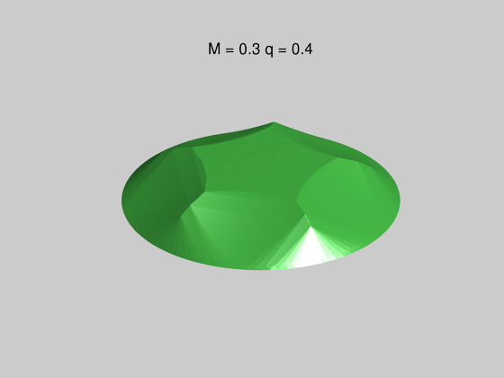
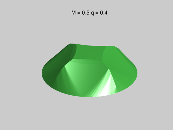
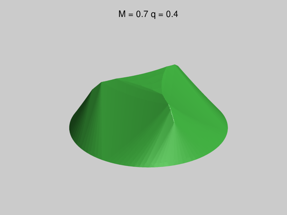
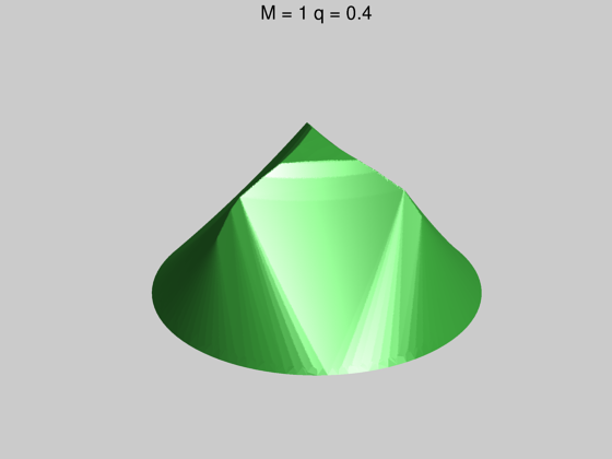
Figure 3. Optimal computed profiles for $q=0.4$ and $M=0.3,\,0.5,0.7,\,1$

Based on this discretization involving only a few parameters $m=50$ (that is $150$ parameters), $d=10$, $n_{c}=100$ and $n=100$ it has been possible to perform in five hours $10^{7}$ evaluations of the discretized cost function on a standard recent laptop. We used the algorithm adaptive_de_rand_1_bin_radiuslimited provided by the BlackBoxOptim library (see [BBO]). We represent in Figure 3, several $q$-concave optimal profiles for the same value $q=0.4$. The observed qualitative behavior is analogous to the one of the solutions computed in [LO] in the case $q=0$:

• Optimal graphs touch the constrained height hyperplane on a curvilinear polygon which seems to be regular. By the way, notice that for $q>0$, there is no flat upper contact anymore. This flat part is replaced by a parabola when $q>0$,

• singular arcs, raising from the vertices of the upper polygon, can be observed in the graph,

• non strictly concave parts of the graph for $q=0$ are substituted by parabolic patches.

7. Appendix: single shock and $q$-concave profiles

The single shock condition reflects the physical fact that every fluid particle hits the body at most once. We shall deduce a corresponding geometric constraint on the body profile. See also [BFK1, CL2, P1].

Let $\Omega\subset\mathbb{R}^{n}$ a bounded convex open set and let $u:\Omega\to\mathbb{R}$ an a.e. differentiable function. We consider a single point particle, moving in $\text{epi }u$ and approaching the graph of $u$ vertically downwards (i.e., along the direction of the coordinate vector $\mathbf{e}_{n+1}$) with constant nonnull velocity $\mathbf{v}=-v\mathbf{e}_{n+1}$, $v>0$. We suppose that the particle hits the graph of $u$ elastically at the point $(x_{0},u(x_{0}))\in\mathbb{R}^{n+1}$, such that $\nabla u(x_{0})$ exists. Furthermore we assume that the particle is reflected according to the usual laws of reflection. Denoting by $\nu_{0}$ the outward normal unit vector at $(x_{0},u(x_{0}))$, i.e.,

$${\nu}_{{0}}:=\left(\frac{-\nabla u(x_{0})}{\sqrt{1+|\nabla u(x_{0})|^{2}}},\frac{1}{\sqrt{1+|\nabla u(x_{0})|^{2}}}\right),$$

we let ${\tau}_{{0}}$ be a vector lying in the subspace of $\mathbb{R}^{n+1}$ generated by ${\mathbf{v}}$ and ${\nu}_{{0}}$, such that ${\nu}_{{0}}\cdot{\tau}_{{0}}=0.$ We denote by $z(t)=({x}(t),y(t))\in\mathbb{R}^{n+1}$, $t>0$, the position of the particle after the shock, occurring at $t=0$. If we consider the components of the velocity vector $z^{\prime}(t)$ along $\nu_{0}$ and $\tau_{0}$, according to the laws of reflection we have to impose

$$\left\{\begin{array}[]{rl}\left[z^{\prime}(t)\cdot{\nu}_{{0}}\right]{\nu}_{{0}}&=-\left({\mathbf{v}}\cdot{\nu}_{{0}}\right){\nu}_{{0}}\\ \left[z^{\prime}(t)\cdot{\tau}_{{0}}\right]{\tau}_{{0}}&=\left({\mathbf{v}}\cdot{\tau}_{{0}}\right){\tau}_{{0}},\end{array}\right.$$

that is,

$$\left\{\begin{array}[]{rl}\left[z^{\prime}(t)\cdot{\nu}_{{0}}\right]{\nu}_{{0}}&=-\left({\mathbf{v}}\cdot{\nu}_{{0}}\right){\nu}_{{0}}\\ z^{\prime}(t)-\left[z^{\prime}(t)\cdot{\nu}_{{0}}\right]{\nu}_{{0}}&={\mathbf{v}}-\left({\mathbf{v}}\cdot{\nu}_{{0}}\right){\nu}_{{0}}.\end{array}\right.$$

So we obtain that

$$z^{\prime}(t) ={\mathbf{v}}-2\left({\mathbf{v}}\cdot{\nu}_{{0}}\right){\nu}_{{0}}={\mathbf{v}}+\frac{2v}{\sqrt{1+|\nabla u(x_{0})|^{2}}}{\nu}_{{0}}=\mathbf{v}+\dfrac{2v}{1+\left|\nabla u(x_{0})\right|^{2}}\left(-\nabla u(x_{0}),1\right)$$

$$=\left(-2\,\frac{\nabla u(x_{0})}{1+|\nabla u(x_{0})|^{2}}\,v\,,\,\frac{1-|\nabla u(x_{0})|^{2}}{1+|\nabla u(x_{0})|^{2}}\,v\right).$$

The trajectory of the particle after the collision is therefore described for $t>0$ by

$$\left\{\begin{array}[]{rl}{x}(t)&=x_{0}-2\,\dfrac{\nabla u(x_{0})}{1+\left|\nabla u(x_{0})\right|^{2}}\,vt\\ {y}(t)&=u(x_{0})+\dfrac{1-\left|\nabla u(x_{0})\right|^{2}}{1+\left|\nabla u(x_{0})\right|^{2}}\,vt.\end{array}\right.$$

The single shock condition at $(x_{0},u(x_{0}))$, which is $u({x}(t))\leq y(t)$ for any $t>0$, is then given by

$$u\left(x_{0}-2\,\dfrac{\nabla u(x_{0})}{1+\left|\nabla u(x_{0})\right|^{2}}\,vt\right)\leq u(x_{0})+\dfrac{1-\left|\nabla u(x_{0})\right|^{2}}{1+\left|\nabla u(x_{0})\right|^{2}}\,vt.$$

If we rescale the time by letting $\tilde{t}_{x_{0}}:=\tfrac{2vt}{1+|\nabla u(x_{0})|^{2}}$, the above inequality rewrites as follows

$$u\left(x_{0}-\tilde{t}_{x_{0}}\nabla u(x_{0})\right)\leq u(x_{0})+\dfrac{\tilde{t}_{x_{0}}}{2}\left(1-|\nabla u(x_{0})|^{2}\right).$$

The above discussion motivates the following

Definition 7.1.

Let $\Omega$ be an open bounded convex subset of $\mathbb{R}^{n}$. We say that $u\colon\Omega\to\mathbb{R}$ is a single shock function on $\Omega$ if $u$ is a.e. differentiable in $\Omega$ and

$$u\left(x-\tau\nabla u(x)\right)\leq u(x)+\dfrac{\tau}{2}\left(1-|\nabla u(x)|^{2}\right)$$

for a.e. $x\in\Omega$ and for every $\tau>0$ such that $x-\tau\nabla u(x)\in\Omega$.

Next we discuss the relation between single shock and $q$-concave profiles. We start by recalling the definition of $q$-concavity.

Definition 7.2.

($q$-concave function) Let $\Omega$ be a convex subset of $\mathbb{R}^{n}$ and $q\geq 0$. A function $u\colon\Omega\to\mathbb{R}$ is said to be $q$-concave on $\Omega$ if the map $x\mapsto u(x)-\tfrac{q}{2}\left|x\right|^{2}$ is concave on $\Omega$. Equivalently, $u$ is $q$-concave on $\Omega$ if and only if

$$u\left(\lambda x+\left(1-\lambda\right)y\right)\geq\lambda u(x)+(1-\lambda)u(y)-\dfrac{q}{2}\lambda(1-\lambda)\left|x-y\right|^{2}$$

for every $x,y\in\Omega$ and for every $\lambda\in[0,1]$.

Lemma 7.3.

Let $q\geq 0$ and $\Omega\subset\mathbb{R}^{n}$ be a bounded convex open set. If $u\colon\Omega\to\mathbb{R}$ is a $q$-concave function on $\Omega$, and $q\,\text{diam}(\Omega)\leq 2$, than $u$ has the single shock property on $\Omega$. In particular, if $u$ is concave then it is single shock in $\Omega$.

Proof..

Let $x\in\Omega$ be such that $\nabla u(x)$ exists, and let $\tau>0$ be such that $x-\tau\nabla u(x)\in\Omega$. Using the $q$-concavity of $u$, the fact that if $x-\tau\nabla u(x)\in\Omega$ then $\tau|\nabla u(x)|\leq\text{diam}(\Omega)$, we have

$$u(x-\tau\nabla u(x)) \leq u(x)+\tau\left(-|\nabla u(x)|^{2}+\dfrac{q\tau}{2}|\nabla u(x)|^{2}\right)$$

$$\leq u(x)+\tau\left(-|\nabla u(x)|^{2}+\dfrac{q}{2}|\nabla u(x)|\,\text{diam}(\Omega)\right)$$

$$\leq u(x)+\tau\left(-|\nabla u(x)|^{2}+|\nabla u(x)|\right)$$

$$=u(x)+\dfrac{\tau}{2}\left(1-|\nabla u(x)|^{2}\right)-\dfrac{\tau}{2}\left(|\nabla u(x)|-1\right)^{2}$$

$$\leq u(x)+\dfrac{\tau}{2}\left(1-|\nabla u(x)|^{2}\right),$$

where we made use of the assumption $q\,\text{diam}(\Omega)\leq 2$. ∎

Remark 7.4.

The inequality $q\,\text{diam}(\Omega)\leq 2$ is sharp. Indeed, if $\Omega$ is a ball, centered at the origin, and $q\,\text{diam}(\Omega)>2$, then the function $\wp_{q}\colon\Omega\to\mathbb{R}$ defined by $\wp_{q}(x):=\tfrac{q}{2}|x|^{2}$ is not a single-shock function on $\Omega.$

Existence of minimizers of the resistance functional on $\mathcal{C}_{q}^{M}(\Omega)$ follows the standard arguments.

Lemma 7.5.

Let $\Omega$ be an open bounded convex subset of $\mathbb{R}^{n}$. Let $M>0$ and $q\geq 0$. Then for every $p\in[1,\infty)$ the class $\mathcal{C}_{q}^{M}(\Omega)$ is compact with respect to the strong topology of $W^{1,p}_{\emph{loc}}(\Omega)$.

Proof.

First of all, a concave function $v$ on $\Omega$ taking values in $[0,M]$ satisfies, for every $K\subset\subset\Omega$,

$$\left|v\left(z_{1}\right)-v\left(z_{2}\right)\right|\leq\frac{2M}{\emph{dist}\,\left(K,\partial\Omega\right)}\left|z_{1}-z_{2}\right|\quad\text{ for every }z_{1},z_{2}\in K.$$

Then, if $R>0$ is such that $\Omega\subset B_{0}(R)$, a $q$-concave function is Lipschitz continuous on any open subset $K$, compactly contained in $\Omega$, with Lipschitz constant not exceeding $\tfrac{2M}{\emph{dist}(K,\partial\Omega)}+qR$.

Let $\left(u_{n}\right)_{n\in\mathbb{N}}$ be a sequence of elements of $\mathcal{C}_{q}^{M}(\Omega)$. We shall prove that there exists a strictly increasing sequence of natural numbers $\left(n_{k}\right)_{k\in\mathbb{N}}$ and $u\in\mathcal{S}_{M,q}(\Omega)$ such that

$$u_{n_{k}}\rightarrow u\text{ in }L^{p}\left(\Omega\right)\text{ e }\nabla u_{n_{k}}\rightarrow\nabla u\text{ in }L^{p}(K)\text{ for every }K\subset\subset\Omega.$$

The sequence $\left(u_{n}\right)_{n\in\mathbb{N}}$ is equi-bounded and equi-Lipschitz on every $K\subset\subset\Omega$. By Ascoli-Arzelà theorem, $\left(u_{n}\right)_{n\in\mathbb{N}}$ admits a convergent subsequence in $C(K)$, for every $K\subset\subset\Omega.$ By a diagonal argument we may obtain the existence of a strictly increasing sequence of natural numbers $\left(n_{k}\right)_{k\in\mathbb{N}}$ and of a function $u\in C(\Omega)$, such that $u_{n_{k}}\to u$ uniformly on each $K\subset\subset\Omega$. Since

$$u\left(\lambda x+\left(1-\lambda\right)y\right) =\lim\limits_{k\to+\infty}u_{n_{k}}\left(\lambda x+\left(1-\lambda\right)y\right)$$

$$\geq\lim\limits_{k\to+\infty}\left[\lambda u_{n_{k}}(x)+\left(1-\lambda\right)u_{n_{k}}(y)-\dfrac{q}{2}\lambda\left(1-\lambda\right)\left|x-y\right|^{2}\right]$$

$$=\lambda u(x)+\left(1-\lambda\right)u(y)-\dfrac{q}{2}\lambda\left(1-\lambda\right)\left|x-y\right|^{2}$$

for every $x,y\in\Omega$ and for every $\lambda\in[0,1]$, $u$ is $q$-concave on $\Omega$. Moreover, since $u_{n_{k}}(x)\in[0,M]$ for every $x\in\Omega$ and for every $k\in\mathbb{N}$, we have $u(x)\in[0,M]$ for every $x\in\Omega$. Thus $u\in\mathcal{C}_{q}^{M}(\Omega)$. Now, since $\Omega$ is bounded and $\left(u_{n_{k}}\right)_{k\in\mathbb{N}}$ is an equi-bounded subsequence, by dominated convergence we infer that $u_{n_{k}}\to u$ in $L^{p}(\Omega).$ In order to conclude we have to show that $\nabla u_{n_{k}}\to\nabla u$ in $L^{p}(K)$ for every $K\subset\subset\Omega$. Since $\left(u_{n_{k}}\right)_{k\in\mathbb{N}}$ is equi-Lipschitz continuous on each $K\subset\subset\Omega$, we have that $\left(\nabla u_{n_{k}}\right)_{k\in\mathbb{N}}$ is equi-bounded on each $K\subset\subset\Omega$. So, it suffices to prove that

$$\nabla u_{n_{k}}(x)\to\nabla u(x)\text{ for a.e. }x\in\Omega.$$

Let $i\in\left\{1,\ldots,n\right\}$ and let $x\in\Omega$ be a fixed point where all $u_{n_{k}}$ $(k\in\mathbb{N})$ and $u$ are differentiable (almost every point of $\Omega$ meets this requirement). Denoting by ${e}_{i}$ the $i$-th vector of the standard basis in $\mathbb{R}^{n}$ and letting $\varphi_{n_{k}}(x):=u_{n_{k}}(x)-\tfrac{q}{2}x^{2}$, since the functions $t\mapsto\varphi_{{n_{k}}}(x+te_{i})$ are concave, there exists $\varepsilon_{0}=\varepsilon_{0}(i,x)>0$ such that, for every $\varepsilon\in(0,\varepsilon_{0})$

$$\dfrac{\varphi_{{n_{k}}}(x+\varepsilon e_{i})-\varphi_{{n_{k}}}(x)}{\varepsilon}\leq\partial_{i}\varphi_{{n_{k}}}(x)\leq\dfrac{\varphi_{{n_{k}}}(x-\varepsilon e_{i})-\varphi_{{n_{k}}}(x)}{-\varepsilon}$$

from which, adding $qx_{i}$ and taking into account that $\partial_{i}\varphi_{u_{n_{k}}}(x)=\partial_{i}u_{n_{k}}(x)-qx_{i}$, we have

$$\dfrac{u_{n_{k}}(x+\varepsilon e_{i})-u_{n_{k}}(x)}{\varepsilon}-\dfrac{q\varepsilon}{2}\leq\partial_{i}u_{n_{k}}(x)\leq\dfrac{u_{n_{k}}(x-\varepsilon e_{i})-u_{n_{k}}(x)}{-\varepsilon}+\dfrac{q\varepsilon}{2}.$$

Passing to the limit as $k\to+\infty$, for every $\varepsilon\in(0,\varepsilon_{0})$ we obtain

$$\dfrac{u(x+\varepsilon e_{i})-u(x)}{\varepsilon}-\dfrac{q\varepsilon}{2}\leq\liminf\limits_{k}\partial_{i}u_{n_{k}}(x)\leq\limsup\limits_{k}\partial_{i}u_{n_{k}}(x)\leq\dfrac{u(x-\varepsilon e_{i})-u(x)}{-\varepsilon}+\dfrac{q\varepsilon}{2}.$$

Passing now to the limit as $\varepsilon\to 0$ we have

$$\partial_{i}u(x)\leq\liminf\limits_{k}\partial_{i}u_{n_{k}}(x)\leq\limsup\limits_{k}\partial_{i}u_{n_{k}}(x)\leq\partial_{i}u(x),$$

that is, $\lim\limits_{k\to+\infty}\partial_{i}u_{n_{k}}(x)=\partial_{i}u(x).$ ∎

Corollary 7.6.

Let $\Omega$ be an open bounded convex subset of $\mathbb{R}^{n}$. Let $M>0$ and $q\geq 0$. The resistance functional $D_{\Omega}$ admits a minimizer on $\mathcal{C}_{q}^{M}(\Omega)$.

Proof.

Notice that, by dominated convergence, functional $D_{\Omega}$ is continuous with respect to the a.e. convergence of gradients. ∎

Acknowledgements

E.M. is member of the GNAMPA group of the Istituto Nazionale di Alta Matematica (INdAM).

References

- [BBO] BlackBoxOptim.jl, a global optimization framework for Julia, https://github.com/robertfeldt/BlackBoxOptim.jl.
- [BFK1] F. Brock, V. Ferone, B. Kawohl, A Symmetry Problem in the Calculus of Variations, Calc. Var. Partial Differential Equations 4 (1996), 593–599.
- [B] G. Buttazzo, A survey on the Newton problem of optimal profiles. In ‘Variational Analysis and Aerospace Engineering’, Volume 33 of the series Springer Optimization and Its Applications (2009), 33-48.
- [BFK2] G. Buttazzo, V. Ferone, B. Kawohl, Minimum problems over sets of concave functions and related questions, Math. Nachr. 173 (1995), 71–89.
- [BG] G. Buttazzo, P. Guasoni, Shape optimization problems over classes of convex domains, J. Convex Anal. 4 (1997), 343–351.
- [BK] G. Buttazzo, B. Kawohl, On Newton’s problem of minimal resistance, Math. Intelligencer 15 (4) (1993), 7–12.
- [CL1] M. Comte, T. Lachand-Robert, Newton’s problem of the body of minimal resistance under a single-impact assumption, Calc. Var. Partial Differential Equations 12 (2001), 173–211.
- [CL2] M. Comte, T. Lachand-Robert, Existence of minimizers for the Newton’s problem of the body of minimal resistance under a single-impact assumption, J. Anal. Math. 83 (2001), 313–335.
- [G] H. H. Goldstine, A history of the calculus of variations from the 17th through the 19th Century. Heidelberg: Springer- Verlag (1980).
- [LO] T. Lachand-Robert, É. Oudet, Minimizing within convex bodies using a convex hull method, SIAM J. Optim. 16 (2005), pp. 368–379.
- [LP] T. Lachand-Robert, M. A. Peletier, Newton’s Problem of the Body of Minimal Resistance in the Class of Convex Developable Functions , Math. Nachr. 226 (2001), 153–176.
- [M] P. Marcellini, Nonconvex integrals of the calculus of variations. In ‘Methods of Nonconvex Analysis’ (Varenna, 1989), Lecture Notes in Math. 1446, Springer-Verlag, Berlin (1990), 16–57.
- [MMOP] E. Mainini, M. Monteverde, E. Oudet, D. Percivale, Newton’s aerodynamic for non convex bodies, to appear on Rend. Lincei Mat. Appl.
- [P1] A. Plakhov, The problem of minimal resistance for functions and domains. SIAM J. Math. Anal. 46 (2014), 2730-2742.
- [P2] A. Plakhov, Newton’s problem of minimal resistance under the single impact assumption. Nonlinearity 29 (2016), 465-488.