Models of Warm Jupiter Atmospheres: Observable Signatures of Obliquity

Abstract

We present three-dimensional atmospheric circulation models of a hypothetical “warm Jupiter” planet, for a range of possible obliquities from 0-90°. We model a Jupiter-mass planet on a 10-day orbit around a Sun-like star, since this hypothetical planet sits at the boundary between planets for which we expect that tidal forces should have aligned their rotation axes with their orbital axes (i.e., ones with zero obliquity) and planets whose timescale for tidal alignment is longer than the typical age of an exoplanet system. In line with observational progress, which is pushing atmospheric characterization to planets on longer orbital periods, we calculate the observable signatures of obliquity for a transiting warm Jupiter: in orbital phase curves of thermal emission and in the hemispheric flux gradients that could be measured by eclipse mapping. For both of these predicted measurements, the signal that we would see depends strongly on our viewing geometry relative to the orientation of the planet’s rotation axis, and we thoroughly identify the degeneracies that result. We compare these signals to the predicted sensitivities of current and future instruments and determine that the James Webb Space Telescope should be able to constrain the obliquities of nearby warm Jupiters to be small (if $\leq 10\arcdeg$) or to directly measure them if significantly non-zero ($\geq 30\arcdeg$), using the technique of eclipse mapping. For a bright target and assuming photon-limited precision, this could be done with a single secondary eclipse observation.

1 Introduction

Exoplanet atmospheric characterization began with a hot Jupiter (Charbonneau et al., 2002) and the majority of all measurements so far have been of the atmospheres of these Jupiter-mass planets that orbit less than 0.1 AU from their host stars. In addition to being inherently interesting, hot Jupiters are the biggest, brightest transiting planets and so the easiest to detect and characterize. However, we are entering an era where transit searches are finding increasing numbers of cooler planets on longer orbital periods and, importantly, ones around bright enough stars that we can extend atmospheric characterization beyond hot Jupiters. This is also facilitated by a better understanding of how to best use current instruments for atmospheric measurements, as well as the much-anticipated launch of new facilities, especially the James Webb Space Telescope. As a field were are poised to expand our understanding of exoplanets to the increasingly diverse possiblities we should expect as we study planets on longer orbital periods.

As of this writing, there are almost three dozen warm Jupiters known to transit their host star, where we define “warm Jupiter” somewhat arbitrarily to mean a planet with a radius greater than 0.5 Jupiter radii and a zero-albedo equilibrium temperature between 500-1000 K. These planets are all around stars bright enough for us to estimate their effective temperatures (necessary to estimate the planets’ equilibrium temperatures). The current brightest planet of this population is WASP-69b, a 1 Jupiter-radius, 0.3 Jupiter-mass planet with an equilibrium temperature of $\sim$960 K around a $V=9.87$ magnitude star (Anderson et al., 2014). The next two brightest, with V magnitudes between 10.5-11 are HAT-P-17b (1 $R_{J}$, 0.5 $M_{J}$, $T_{eq}\sim 790$ K, and $e=0.34$; Howard et al. 2012) and WASP-84b (0.9 $R_{J}$, 0.7 $M_{J}$, and $T_{eq}\sim 800$ K; Anderson et al. 2014). We expect that this population of known warm Jupiters should grow as current transit searches continue and new ones begin. In particular, missions such as the Transiting Exoplanet Survey Satellite (TESS) and the PLAnetary Transits and Oscillations of stars (PLATO) satellite should identify more planets that transit bright stars, improving our ability to characterize these worlds.

A significant difference between the populations of “warm” and “hot” Jupiters is that the overwhelmingly strong tidal forces experienced by hot Jupiters will no longer be so overwhelming for the longer orbital period, warm population. As a consequence, whereas we generally assume that the rotation rates of hot Jupiters are synchronized with their orbital rates and their rotation axes are aligned with their orbital axes, these assumptions no longer hold for warm Jupiters and we should expect a range of possible values for these parameters. One observable expression of this decreasing influence of tidal forces on longer period planets is the increase in their range of orbital eccentricities (see review by Winn & Fabrycky, 2015). As we expand observational and theoretical efforts out from hot Jupiters there are three planetary properties that were fixed for the hot Jupiter population, but that we should expect to create additional diversity among the longer period “warm Jupiters”: eccentricity, rotation rate, and obliquity. There has been previous work studying different eccentricities (Kataria et al., 2013) and rotation rates (Showman et al., 2015) for warm Jupiters; here we focus on non-zero obliquities.

Previous work studying non-zero obliquities of exoplanets has generally fallen into one of two main categories. The first includes papers that study the influence of obliquity on atmospheric circulation patterns, often with an emphasis on Earth-like planet and their habitability (e.g., Williams et al., 1996; Williams & Pollard, 2003; Spiegel et al., 2009; Ferreira et al., 2014; Linsenmeier et al., 2015; Shields et al., 2016). The second category contains papers that identify means by which we may be able to measure or constrain the obliquities of exoplanets, either using a presumed atmospheric state or analytic models that allow for any general spatial pattern. Seager & Hui (2002) demonstrated that the oblateness of a planet, due to rotation, can impart a small signal on its transit light curve, and the obliquity of the planet influences the shape and strength of this feature. This method was subsequently used to observationally constrain the oblateness of several exoplanets and a brown dwarf companion (Carter & Winn, 2010; Zhu et al., 2014). There have also been studies of ways to constrain a transiting or directly imaged planet’s obliquity with future instrumentation, including signatures of obliquity within scattered light curves (Kawahara & Fujii, 2010; Kawahara, 2016), polarimetric observations (de Kok et al., 2011), and the planet’s Rossiter-McLaughlin effect during secondary eclipse (Nikolov & Sainsbury-Martinez, 2015).

In a more general approach, Cowan et al. (2013) and Schwartz et al. (2016) presented useful analytic frameworks for identifying how the intrinsic properties of exoplanets (e.g., their rotation rates, inclinations, obliquities, albedos, etc.) couple with the extrinsic viewing orientation (related to the planet’s orbital parameters) in order to shape observed orbital and rotational photometric variations, for emitted or reflected light. They explicitly identified how the spatial information on the planet is expressed in the temporal information of the light curve, as well as which spatial patterns are necessarily (i.e., mathematically) invisible in these light curves.

Gaidos & Williams (2004) is a rare work that fits within both categories of obliquity research; they simulated the influence of non-zero obliquity (as well as non-zero eccentricity) on a planet’s atmospheric structure, using energy balance models (considering a range of thermal inertias), and also predicted observable consequences, calculating thermal phase curves as a function of viewing orientation. While these authors focused on terrestrial planets with Earth-like temperatures, some of their results regarding the influence of viewing orientation on observed seasonality are reproduced in our predictions, as we will describe below. They also found significant degeneracy between the effects of obliquity, thermal inertia, and viewing orientation; we uniquely identify secondary eclipse maps as a means by which we may be able to break these degeneracies. In addition, our atmospheric model is more complex and the thermal inertia is not an input but a prediction (albeit influenced by other, more basic, planetary parameters we choose). Cowan et al. (2012) expanded on this by using two detailed three-dimensional circulation models for the Earth (one similar to current-day conditions and one representative of a snowball state) to simulate orbital thermal phase curves, as viewed from different orientations. While they did not vary obliquity or eccentricity, their models did include self-consistent heat transport and so could test the influence of thermal inertia by comparing their temperate and snowball models.

In this work we identify the next set of observable planets whose obliquities may be measurable (“warm Jupiters”) and present a joint analysis of their atmospheric state and observability (both via thermal phase curves and eclipse maps). We start our exploration of non-zero obliquities by modeling a hypothetical Jupiter-like planet on a 10-day orbit around a Sun-like star. We choose this orbital period because it corresponds to where the timescales for tidal circularization and axial alignment (which are of similar magnitude, e.g. Peale, 1999) may be comparable to the typical lifetime of an exoplanet system. Starting with the timescale for tidal spin-down of a planet (Guillot et al., 1996), $\tau$, and solving for the planet’s orbital period, we find:

$$P\sim\left(\frac{\tau}{Q}\frac{16\pi^{4}R_{p}^{3}}{G\omega_{p}M_{p}}\right)^{1/4}.$$ (1)

This formulation disguises any complexity of the planet’s tidal dissipation by using a single parameter, $Q$, and we are also ignoring any orbital changes that may happen over time, so we can use this to estimate the orbital period at which the timescale for tidal effects may be comparable to the age of the system (setting that equal to $\tau$), but this is not a strict prediction for a specific boundary in physical conditions. Nevertheless, using the mass, radius, and current spin of Jupiter (as an estimate for the initial spin rate, $\omega_{p}$), an estimate for the tidal dissipation factor of $Q\sim 10^{6}$, and assuming an age on the order of Gyr, we solve for an orbital period of $P\sim 10$ days. This is then roughly the orbit at which we would not know whether or not to expect that tidal forces should have aligned a planet’s obliquity, and so this presents an interesting potential target for characterization.

The equilibrium temperature for a planet on a 10-day orbit around a Solar analog is $\sim$900 K. Interestingly, this is near the $\sim$1000 K boundary identified by Thorngren et al. (2016), cooler than which we may be able to assess the metallicities of exoplanets from their bulk densities, without the (still unknown) hot Jupiter radius inflation mechanism confusing matters. In other words, the planets that we may want to study in order to answer fundamental questions about planet bulk compositions are also those planets for which we should expect a range of non-zero obliquities.

In this paper we compare models for a hypothetical warm Jupiter at different obliquities using a three-dimensional General Circulation Model (GCM). In Section 2 we discuss our modeling framework, including the treatment for non-zero obliquity. In Section 3 we present the results from the GCM and discuss the variation in circulation patterns between models. We show observable properties of each model in Section 4: the thermal phase curves (4.1) and eclipse maps (4.2). We also compare these predicted signals to the sensitivities of current and future instruments (4.3). Finally, in Section 5 we summarize our results and the potential for observationally constraining the obliquities of warm Jupiters.

2 Atmospheric Circulation Model

We present three-dimensional atmospheric circulation models for a hypothetical planet with the mass, radius, and rotation rate of Jupiter, on a 10-day period orbit around a Sun-like star. We calculated the circulation patterns using a numerical code that solves the primitive equations of meteorology, with pressure as the vertical coordinate, and uses a double-gray scheme for the radiative transfer, as described thoroughly in Rauscher & Menou (2012). This code has been updated to allow for the variable stellar irradiation patterns appropriate for planets with non-zero obliquity, as described in Section 2.1 below. We ran models for obliquities from 0 to 90°, with all other physical parameters remaining the same (as listed in Table 1). Specifically, we simulated planets with obliquities of: 0°, 3° (equal to Jupiter’s obliquity), 10°, 30° ($\approx$ the obliquities of Earth, Saturn, and Neptune), 60°, and 90° (close to Uranus’ obliquity). We chose values for the gray optical and infrared absorption coefficients such that the analytic solution (Guillot, 2010) roughly matches the temperature-pressure profile for a hypothetical Jupiter-like planet at 0.1 AU, as calculated from a one-dimensional atmospheric model with detailed radiative transfer (Fortney et al., 2007).

Table 1: Model physical parameters

Parameter	Value
Radius of the planet, $R_{p}$	$6.986\times 10^{7}$ m
Gravitational acceleration, $g$	26 m s-2
Orbital revolution rate, $\omega_{\mathrm{orb}}$	$7.2722\times 10^{-6}$ s-1
Corresponding period, $P_{\mathrm{orb}}$	10 day⊕
Rotation rate, $\omega_{\mathrm{rot}}$	$1.7587\times 10^{-4}$ s-1
Corresponding period, $P_{\mathrm{rot}}$	10 hours
Incident flux at substellar point, $F_{0}$	$1.36\times 10^{5}$ W m-2
Corresponding temperature, $T_{\mathrm{irr}}$	1250 K
Internal heat flux, $F_{\uparrow\mathrm{IR},\mathrm{int}}$	5.7 W m-2
Corresponding temperature, $T_{\mathrm{int}}$	100 K
Optical absorption coefficient, $\kappa_{\mathrm{vis}}$	$2.6\times 10^{-3}$ cm2 g-1
Optical photosphere ($\tau_{\mathrm{vis}}=2/3$)	667 mbar
Infrared absorption coefficient, $\kappa_{\mathrm{IR},0}$	$5.2\times 10^{-2}$ cm2 g-1
Infrared photosphere ($\tau_{\mathrm{IR}}=2/3$)	33 mbar
Specific gas constant, $\mathcal{R}$	3523 J kg-1 K-1
$\mathcal{R}/c_{P}$	0.2857

Our standard model runs were performed at a horiztonal spectral resolution of T42 (corresponding to $\sim$3° resolution at the equator) and with 30 vertical levels evenly sampled in $\log P$ from 100 bar to 1 mbar. We applied numerical hyperdissipation as an eighth-order operator on the wind and temperature fields (as described in Rauscher & Menou, 2012), with a dissipation timescale of 0.02 $P_{\mathrm{rot}}$, which we found to adequately remove noise at the smallest scales without overdamping the kinetic energy spectrum of the circulation. We initialized the models using a horizontally uniform temperature profile, whose vertical (pressure) dependence was set to match the globally averaged analytic solution for our double-gray opacities (Guillot, 2010). We started each run with the winds at rest and used 360 timesteps per $P_{\mathrm{rot}}$ to simulate each planet for 3000 orbital periods ($=72552$ $P_{\mathrm{rot}}$), by which point the winds throughout the observable atmosphere had finished accelerating (for yearly averaged values).

We can calculate the expected scale of dynamical features in our planet’s global circulation using the Rossby deformation radius (e.g., Showman et al., 2010) and find that at the infrared photosphere this scale is $\sim$8°. While T42 resolution should be sufficient to capture these features, we tested some limited models at T63 and T85, corresponding to $\sim$2° and $\sim$1.4° resolutions, respectively. We found very similar circulation patterns and temperature structures, without any smaller scale detail emerging in these higher resolution runs, giving us confidence that the T42 resolution is sufficient to model the global circulation pattern of this planet.

One unavoidable concern when modeling planetary atmospheres is whether there could be sub-grid physics, not captured within the numerical simulation, that could influence the global circulation of the planet. While this may be of particular concern for hot Jupiters, where the intense stellar irradiation can drive super-sonic winds, potentially triggering sub-grid shocks and hydrodynamic instabilities (e.g., Li & Goodman, 2010; Fromang et al., 2016), these particular effects should be less important in the calmer atmospheric circulation of warm Jupiters. (To preview our results: the maximum wind speeds we find are about 1 km s^-1, whereas the sound speeds in the atmosphere range from 2-3 km s^-1.) Nevertheless, we are fundamentally not resolving whatever form of sub-grid dissipation exists in these atmospheres, instead capturing it through our hyperdissipation parameter. As there is no a priori physical basis for calculating this parameter (Cho & Polvani, 1996), our uncertainty in the correct value to use could, for example, result in errors in our maximum wind speeds (Heng et al., 2011). Mayne et al. (2014) also has a nice discussion of the implications of this and other assumptions used in hot Jupiter circulation modeling. While issues of sub-grid physics are not unique to our models, and perhaps may be better behaved than in the hot Jupiter context, this is an important caveat that should be kept in mind.

2.1 Stellar Flux Pattern for Non-zero Obliquities

Our atmospheric circulation code has been used before to model the atmospheres of planets with zero obliquity, for a variety of stellar heating patterns. In the case of hot Jupiters the stellar heating pattern does not change with time (in the frame rotating with the planet). The flux has a maximum at the substellar point, falls off as the cosine of the angle from the substellar point, and is zero everywhere on the planet’s perpetual nightside. In the case of non-synchronous rotation (as in Rauscher & Kempton, 2014) the same hemispheric forcing pattern is used, but the longitude of the substellar point varies with time. If the planet is rotatingly quickly enough that the time between consecutive star-rises is shorter than the radiative timescale of the atmosphere, it is more appropriate to use a diurnally averaged stellar heating pattern, such that the equator receives more flux than the poles (for zero obliquity). This was the forcing pattern we used for the models presented in May & Rauscher (2016).

Here we have updated our code to calculate the appropriate stellar forcing patterns for planets with non-zero obliquities. For these planets the latitude of the substellar point ($\phi_{\mathrm{ss}}$) has a yearly seasonal dependence given by:

$$\sin\phi_{\mathrm{ss}}=\sin\psi\sin(2\pi t/P_{\mathrm{orb}}),$$ (2)

where $\psi$ is the planet’s obliquity and the zero-point for time in the orbit ($t=0$) is set to be the vernal equinox in the Northern hemisphere, such that the maximum Northern excursion of the substellar latitude ($\phi_{\mathrm{ss}}=+\psi$) occurrs at the Northern summer solstice ($t=0.25P_{\mathrm{orb}}$). If the planet is rotating quickly enough that it is appropriate to use a diurnally averaged stellar flux pattern to heat the atmosphere, the downward flux at the top of the atmosphere can be calculated as (e.g., Liou, 1980):

$$F(\phi)=\frac{F_{o}}{\pi}(\sin\phi\sin\phi_{\mathrm{ss}}\ H+\cos\phi\cos\phi_{\mathrm{ss}}\sin H),$$ (3)

where $F_{0}$ is the incident flux at the substellar point and $H$ is the length of half a day (from star-rise to noon), measured in radians, for the given latitude: $H=\cos^{-1}(-\tan\phi\tan\phi_{\mathrm{ss}})$. The inverse cosine function is only defined when its argument is within $[-1,1]$. For latitudes greater/lesser than the substellar latitude during Northern/Southern summer, $H=\pi$ and those regions of the planet experience perpetual daylight for the season, while similarly there are latitudes in the other hemisphere that will have $H=0$ and experience seasonally perpetual nighttime.

Since we assume Jupiter’s rotation rate for our hypothetical planet, and a 10-day orbit around a Sun-like star, we can use the prescription in Showman et al. (2015) to determine the appropriateness of using a diurnally averaged stellar heating pattern in this case. We do find that the radiative timescale at the optical photosphere (the $\tau=2/3$ surface for absorbed starlight) is greater than the rotation period (favoring a diurnal average), but only by a factor of $\sim$2. We tested the impact of using a diurnal stellar heating pattern by performing limited versions of our zero and 90° obliquity models in which we explicitly move the heating pattern with time. In order to correctly model the movement of the substellar point, it should not advance more than one grid point in one timestep. For the case of zero obliquity, this is equivalent to requiring that the number of timesteps per $P_{\mathrm{rot}}$ is greater than the number of longitude points (128 at our standard T42 resolution) times the number of timesteps between each time the radiative transfer routine is calculated (10), times the number of rotation periods in an orbital period minus one ($24.184-1$). This minimum requirement forces us to use 30000 timesteps per rotation period, a factor of almost 100 greater than (and so computationally slower than) our standard runs. We found that the atmospheric structure in these models was still mostly axisymmetric, with wind and temperature patterns that look very similar to those from the models with diurnally averaged heating patterns. The deviations from axisymmetry were very small; for example, at the infrared photosphere the temperatures in a single latitude circle are always within 2% of the average at that latitude. This supports the use of a diurnal average for this planet’s heating pattern.

3 Comparison of circulation patterns

Our models with relatively low obliquity (0°, 3°, and 10°) all exhibit atmospheric structures where the equator is warmer than the poles and the circulation is eastward throughout most of the atmosphere, dominated by a jet at high latitude in each hemisphere. The $\psi=0\arcdeg$ and $\psi=3\arcdeg$ models are largely indistinguishable, so much so that we do not find it worthwhile to present results from the 3° model. Between the 0° and 10° models there are only small differences in wind speed and jet width. In Figure 1 we show plots of the zonally averaged zonal wind (in the East-West direction) for each model; the plots for the 0° and 10° models are yearly averages, since little-to-no seasonal variation is observed, while for the higher obliquity models several snapshots are shown throughout the planet’s year.

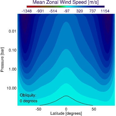
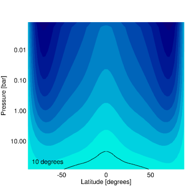
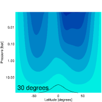
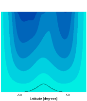
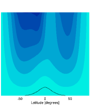
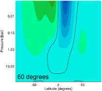
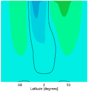
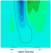
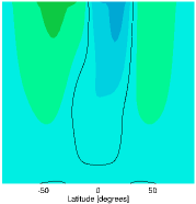
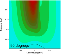
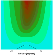
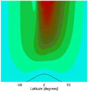
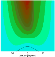
Figure 1: The zonally averaged zonal (East-West) winds for models with obliquities of: 0° (top left), 10° (top right), 30° (third row from the bottom), 60° (second row from the bottom), and 90° (bottom row). The plots for $\psi=0\arcdeg$ and $\psi=10\arcdeg$ are annual averages; the other plots are snapshots at: (Northern) vernal equinox, summer solstice, autumnal equinox, and winter solstice (left to right). The colorscale is the same for each plot and the black line is boundary between Eastward (positive) and Westward (negative) winds.

For this hypothetical planet, we find that significant seasonal differences emerge once the obliquity reaches 30°, with a clear shift in wind patterns and temperature structure as the Northern and Southern hemispheres receive more or less direct heating. The circulation pattern for the $\psi=30\arcdeg$ model resembles the patterns for lower obliquity models, with dominant eastward flow and high latitude jets, but the jet structure is slightly distorted between the two hemispheres, with a seasonal dependence. The flow patterns for the $\psi=60\arcdeg$ and $\psi=90\arcdeg$ models also show a seasonal dependence, but the winds in these models are significantly different from the lower obliquity cases. For $\psi=60\arcdeg$ there is a more even distribution between eastward and westward winds and the flow is characterized by an eastward jet that remains near the equator, but shifts up and down in latitude seasonally. The 90° obliquity model is dominated by westward flow, with a strong jet at the equator that shifts slightly in latitude throughout the year. These planets are clearly in a different circulation regime than lower obliquity planets.

In Figure 2 we show how the temperature structures of the $\psi\geq 30\arcdeg$ models respond to the changing seasons. We plot the temperature at the infrared photosphere for each of these models as a function of time, throughout one orbit of the planet. For each model we plot the latitudinal temperature structure by taking an azimuthal average (as is appropriate since our diurnal heating pattern results in no significant variation of properties with longitude). On top of these temperature contours we plot a dashed black line to show the latitude of the substellar point as a function of time (Equation 2), so that we can compare the spatial and temporal response of the atmosphere to the changing irradiation pattern.

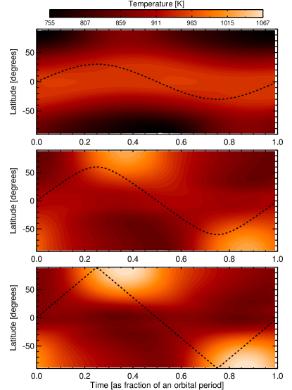
Figure 2: The latitudinal temperature structure at the infrared photosphere (red contours, with color scale at top) and the latitude of the substellar point (black dashed line, Equation 2), as a function of time throughout one orbit of the planet. From top to bottom the panels show results for the models with 30°, 60°, and 90° obliquity, respectively. In all models the temperature structure lags the stellar irradiation pattern, with a timescale of $\sim$1/8 $P_{\mathrm{orb}}$.

For the $\psi=30\arcdeg$ model the temperature structure is similar to that of lower obliquity models, in that the equator remains warmer than the poles, but the latitude of maximum temperature shifts above and below the equator with time. The stark change in atmospheric regime between the $\psi\leq 30\arcdeg$ and $\psi\geq 60\arcdeg$ models seen in the wind patterns (Figure 1) is also reflected in the temperature structures. At most times during the year one hemisphere is significantly warmer than the other, such that the main temperature gradient is between the summer and winter hemispheres, with short times of relatively uniform temperature near the equinoxes.

From Figure 2 we can also see that the atmospheres of the $\psi=30\arcdeg$, 60$\arcdeg$, and 90$\arcdeg$ models all respond to the changing irradiation pattern with a similar response time. This is observed as a lag in the latitude of the maximum temperature, relative to the substellar latitude, by $\sim$1/8 $P_{\mathrm{orb}}$. This response time is about an order of magnitude longer than the radiative timescale at the infrared photosphere ($\sim$0.014 $P_{\mathrm{orb}}$), evidencing a complex radiative and dynamical response of the atmosphere as it transports energy from the heating at the optical photosphere (where the radiative timescale is also shorter than the response time, at $\sim$0.05 $P_{\mathrm{orb}}$).

The focus of this paper is the observable consequences of non-zero obliquities and so a more detailed analysis of these circulation patterns and the shift between regimes will have to wait for future work. The take-away point from this section is that seasonal effects are insignificant for our models with obliquities $\leq 10$°, but influence the temperature structure at the infrared photosphere (i.e., what we would see in thermal emission) for models with obliquities $\geq 30$°.

4 The effect of obliquity on observable properties

The nature of any observable seasonal variation will depend not only on the intrinsic physical properties of the system (e.g., $P_{\mathrm{orb}}$, $\psi$, stellar flux, etc.), but also on the extrinsic viewing orientation of the observer relative to the planet’s axial tilt, which can be characterized by the coordinates of the subobserver point. Since we are considering diurnally averaged models here, all subobserver longitudes are equal. The subobserver latitude, $\phi_{\mathrm{obs}}$, sets the viewing orientation and remains constant with time; it is related to the obliquity and observed orbital phase ($\gamma$) as:

$$\sin\phi_{\mathrm{obs}}=\sin\psi\sin(2\pi[\gamma-t/P_{\mathrm{orb}}])$$ (4)

where $t=0$ is the same as in Equation 2. Transit is defined to occur at an orbital phase of $\gamma=0,1$ and secondary eclipse is at $\gamma=0.5$ (assuming a transiting system and a circular orbit). Since the seasonal orientation of any system is a priori unknown, Equation 4 allows us to analyze output from our models for fixed observer orientations ($\phi_{\mathrm{obs}}$), snapshots from the simulation ($t/P_{\mathrm{orb}}$), or orbital phases. A full phase curve observation occurs over a planet’s year ($\Delta t=P_{\mathrm{orb}}$) and requires a choice for the viewing orientation.

For an eclipse mapping observation (at $\gamma=0.5$), we need to know not just the subobserver latitude, but in which direction the pole of the planet is pointed. Using the spherical law of cosines (following the example of Schwartz et al., 2016), we find that the angle, $C$, through which the Northern pole should be rotated (in a clockwise direction) around a line that passes from the center of the planet to the observer (through the subobserver point), is given by:

$$\cos C=\cos\psi/\cos\phi_{\mathrm{obs}}.$$ (5)

Cosine is an even function and the solution for $C$ could be a positive or negative value; these correspond to the two points during a planet’s orbit when an observer might be oriented such that secondary eclipse occurred at that value of $\phi_{\mathrm{obs}}$. From a consideration of the orbital geometry (using Equation 4) it is apparent that the positive solutions correspond to $-1/4<t/P_{\mathrm{orb}}<1/4$ and the negative solutions to $1/4<t/P_{\mathrm{orb}}<3/4$.

4.1 Orbital thermal phase curves

In the simulated orbital phase curves presented here we assume that our hypothetical planet is of interest because it transits and we choose to view the system exactly edge-on. This allows us to isolate the observable consequences of non-zero obliquities, but for actual systems these effects would be convolved with the effect of viewing at an orbital inclination slightly less than exactly 90°. This will be a minor effect and in practice the orbital inclination is measurable from the shape of the transit curve and so the reference frame could be adjusted to account for this angle.

Since we force the orbital inclination of our hypothetical system to be exactly edge-on to the observer, this constrains the possible viewing geometry such that the planet must be seen with a subobserver latitude ranging from zero to $\pm\psi$ (and for the zero obliquity model this means that the planet is also always viewed exactly along its equator). We calculate a set of simulated phase curves for each of our models by assuming various orientations (i.e. using different values for the subobserver latitude in Equation 4), and then integrate the flux emitted from the hemisphere facing the observer, as a function of time throughout one orbit, as the planet undergoes seasonal changes. It is necessary to simulate a set of curves for each non-zero obliquity model because the random orientation of the observer relative to the system will directly affect the measured phase curve, as seen in Figure 3. Figure 4 shows maps of the flux emitted from each of our models, oriented for the different viewing geometries used to produce the curves in Figure 3. Each map is for a snapshot of the planet at an orbital phase of zero; full-orbit movies showing the seasonal flux variation for the cases shown in Figure 4 are available as supplemental files.

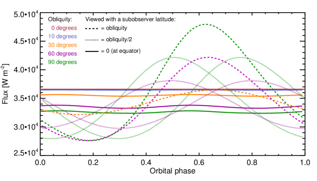
Figure 3: Orbital phase curves for models with a range of obliquities. These curves show the amount of flux that the planet is emitting, from the hemisphere facing a distant observer, as a function of time throughout the planet’s orbit. Not only does the amount of flux differ between models with different obliquities (shown as different colors), but the observed flux variation from any particular model depends on the orientation with which the observer is viewing the planet (shown as different line styles). Maximal variation would be seen if the axis of the planet is tilted toward the observer such that one hemisphere is primarily in view ($\phi_{\mathrm{obs}}=\psi$), whereas the least variation is seen if the planet’s axis is perpendicular to the observer such that equal parts of the Northern and Southern hemisphere are in view ($\phi_{\mathrm{obs}}=0$). In all cases the geometry of the system is assumed to be transiting; secondary eclipse would occur at the orbital phase 0.5 (when the observed planet flux drops to zero as it passes behind its star, but not included in these curves). The corresponding planet emission flux maps for each curve are shown in Figure 4 and full-orbit movies are available as supplemental files.

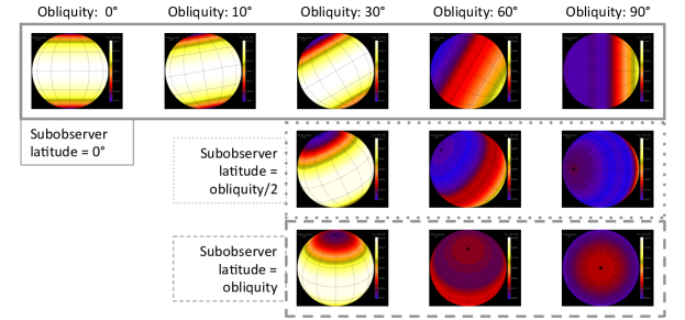
Figure 4: Maps of the flux emitted from models with various obliquities (from left to right, as labeled), and as observed with different viewing orientations. In all cases the planet is assumed to be in a transiting orbit and these images are for the time when $\gamma=0$, meaning that the planet would be at the center of transit. The top row show the planet as it would look if the equator of the planet was aligned toward the observer. The middle row show the planet as if the observer were seeing the planet at a latitude equal to half of the planet’s obliquity (so at 15$\arcdeg$ for the $\psi=30\arcdeg$ model, 30$\arcdeg$ for the $\psi=60\arcdeg$ model, and 45$\arcdeg$ for the $\psi=90\arcdeg$ model). The bottom row shows the planet oriented such that its rotation axis is pointed toward the observer, so that the observer views a latitude equal to the obliquity. Movies showing the time variation of this flux pattern throughout the planet’s orbit, for all models and viewing orientations represented here, are available as supplemental files.

If our hypothetical planet has zero obliquity, then its orbital phase curve should be completely flat. Its temperature structure is axisymmetric (due to its assumed Jupiter-like rotation rate and diurnally averaged stellar heating pattern) and it experiences no seasonal variations, so the emitted flux is constant with time, as seen in Figure 3. We can compare the flux level of this curve to the flux level that we would expect if the heating from the star was evenly re-radiated from the entire planet surface, ($F_{\mathrm{irr}}/4=3.4\times 10^{4}$ W m^-2). We find that the flux from our $\psi=0\arcdeg$ model is lower than this global average, which is not surprising. Atmospheric transport does not completely homogenize the equator-to-pole temperature difference from differential heating, leaving the equator hotter than the global average, and we preferentially observe this brighter region of the planet. If we could independently constrain the obliquity of a planet to be zero, then the flux level of the orbital phase curve would be a measure of the efficiency of equator-to-pole heat transport, with values closer to the globally averaged flux meaning more efficient transport.

In the case that it cannot be measured independently, the obliquity of the planet has a degenerate effect with the equator-to-pole heat transport on the observed flux level, for equatorial viewing geometries. Figure 3 shows that—at equatorial viewing orientations—a lower level of emitted flux is associated with a higher value of planetary obliquity. Values less than the globally averaged incident flux ($3.4\times 10^{4}$ W m^-2) are observed for planets with obliquities $\geq 60$°, a result of the poles of these planets receiving more flux than the equator, integrated over an orbit. Figure 2 shows that these high obliquity models have equatorial temperatures that are always equal to or less than the planet’s average temperature. When the planet is observed along the equator we preferentially see these cooler regions and so the average hemispheric flux is decreased relative to the lower obliquity models.

The phase curves for equatorial viewing geometry are not completely flat; there is some small amount of seasonal variation (similar to the semi-orbital variations in the blackbody planet models of Gaidos & Williams, 2004). Even though an observer would see an equal amount of each hemisphere, Figure 2 shows that there are times of the year when one hemisphere is much hotter than average and times when both hemispheres are both only warm, leading to an integrated flux level that shows a small amplitude seasonal variation. However, this signal would likely be lost in the noise of an actual phase curve measurement (see Section 4.3) and so these curves are effectively flat.

The take-away point from the solid curves in Figure 3 is that if we observe a flat phase curve for the thermal emission from a transiting planet, we are probably observing the planet along its equator. If the measured flux level is above the globally averaged value ($F_{\mathrm{irr}}/4=\sigma T_{\mathrm{star}}^{4}[R_{\mathrm{star}}/2a]^{2}$), then the planet’s equator is hotter than its poles and the obliquity is likely less than 54°. In this case the measured flux level is giving us information about the efficiency of equator-to-pole heat transport. If the observed flux is below the globally averaged value, then the obliquity is likely greater than 54° and our results show that lower levels correspond to higher obliquities. An important caveat to this is that the albedo of the planet may be unknown, in which case the globally averaged flux value would need to be adjusted down by an unknown amount, confusing the interpretation of a flat phase curve.

The set of flat (or effectively flat) solid phase curves shown in Figure 3 are for the particular viewing orientation of the subobserver point being along the planet’s equator. Plotted as dashed lines in Figure 3 are the other extreme viewing orientation, where the planet is observed at the maximum possible subobserver latitude (for a transiting system), $|\phi_{\mathrm{obs}}|=\psi$. For these cases we observe the maximum variation in emitted flux, since the full seasonal response of a hemisphere is preferentially in view. Without spatially resolving the planet from the star we cannot know the orientation of the orbital angular momentum vector, leading to a North-South degeneracy in our observed properties. We do not know whether our subobserver latitude is positive or negative (Northern or Southern), but since both hemispheres respond to the seasonal cycle symmetrically, it is only the absolute value of $\phi_{\mathrm{obs}}$ that is relevant anyway.

For the $\psi=10$° model, which does not show significant seasonal variation, the $\phi_{\mathrm{obs}}=\pm 10$° viewing orientation results in a slightly diminshed flux level. This is simply explained by the higher latitudes on the planet being cooler than the equator and so shifting those latitudes to greater visibility diminishes the disk-integrated flux observed. For the models that do exhibit seasonality ($\psi=30,60,90$°) the amplitude of variation increases for increasing obliquity, while the orbital phase of the maximum flux is the same for all models. This trend of increasing variation with obliquity was also found for Earth-like planets in Gaidos & Williams (2004), and their results can also be used to make sense of the constant phase we see for maximum flux, since the thermal inertia of the atmosphere is the same for all models.

When we observe the planet at $\phi_{\mathrm{obs}}=\psi$, then according to Equations 2 and 4, the solstice for the hemisphere facing us occurs at $\gamma=0.5$ and so the phase difference between this and the peak flux is a measure of the atmospheric response time to the changing irradiation pattern. This agrees with the peak of the curves in Figure 3 being at 0.5 $+\sim$1/8 $\approx 0.625$, matching the timescale for atmospheric response determined above (see Section 3).

In the bottom plot of Figure 3 we show intermediate viewing angles for the highest obliquity models ($\psi=60,90$°), those with the strongest seasonal variation. When $\phi_{\mathrm{obs}}\neq\psi$ two solutions exist for the orientation of the observer relative to the system. When $\phi_{\mathrm{obs}}=0$°, as in the solid curves of Figure 3, these two solutions produce overlapping phase curves because of hemispheric symmetry, but at intermediate values they do not, as is evident in the $\phi_{\mathrm{obs}}=\psi/2$ curves shown as dotted lines. For one solution the planet is observed such that solstice in the primarily observed hemisphere occurs before $\gamma=0.5$ and in the other solution it occurs after $\gamma=0.5$, resulting in phase shifts in either direction. The phase at which peak flux occurs depends on a combination of the atmospheric response timescale and the subobserver latitude, with a positive or negative shift depending on which orientation we are observing from, relative to the seasonal cycle.

In general we have learned that the orbital phase curves of emitted light from this hypothetical planet contain information about the planet’s intrinsic properties of obliquity, and either equator-to-pole heat transport (for low obliquity), or the atmospheric timescale for seasonal response (for high obliquity). The expression of these properties is regulated by the viewing orientation of the system, which could make it difficult to disentangle the intrinsic information without some other independent constraint on the viewing or inherent properties (confirming the conclusions of Gaidos & Williams, 2004). However, if the planet obliquity or viewing geometry were known, then we could constrain atmospheric properties through the type of analysis demonstrated here. In the next Section we discuss another type of measurement that could be done instead, or could be used to break the degeneracies in the phase curves.

4.2 Eclipse maps

Orbital phase curves have been the primary means by which we have measured spatial information about exoplanets but, as we just saw, this type of observation should become less informative (and much more time-consuming) for planets on longer orbital periods. Conveniently, another type of observational technique, known as eclipse mapping, should be increasingly useful for longer period planets. In this method, the detailed shape of the flux curve as the planet passes into secondary eclipse (ingress) or comes out from behind the star (egress), can be inverted to construct a two-dimensional map of the planet’s dayside brightness pattern (Williams et al., 2006; Rauscher et al., 2007; de Wit et al., 2012; Majeau et al., 2012). The advantages of using this method for longer period planets are:

• It only requires observation during the time surrounding secondary eclipse, requiring much less telescope time than a full orbit (which would be 10 days for our hypothetical planet).

• The slower orbital speed of the planet means that the ingress and egress take longer, providing a better opportunity to characterize the detailed shape of this part of the light curve.

• The two-dimensional information retrieved by this method can constrain multiple properties of the planet. In addition to the magnitude of the equator-to-pole or North-to-South temperature gradient, the orientation of the flux gradient can reveal information about the planet’s obliquity.

The primary measurement made during secondary eclipse is the total decrement in light when the planet is blocked from view, behind the star. The total depth of the eclipse then gives us the integrated flux from the dayside hemisphere of the planet. From Figure 3 we can see that the amount of planetary flux that would be eclipsed by the star (the value of each curve at an orbital phase of 0.5) can depend strongly on the obliquity of the planet and the viewing orientation, but degeneracies exist such that these two properties cannot be uniquely retrieved. For example, in Figure 3 some of the curves for the $\psi=60\arcdeg$ model would be observationally indistinguishable from some curves for the $\psi=90\arcdeg$ model at 0.5 orbital phase; many more overlapping possibilities exist for the full range of obliquities and viewing geometries. The secondary eclipse depth alone does not provide a strong constraint on the planet’s obliquity.

Eclipse mapping provides the additional information required to discriminate between the temperature structures of low- or high-obliquity planets, in the case where they have the same hemispherically integrated flux. In Figure 5 we show the temperature map at the infrared photosphere for the 60° obliquity model, at several snapshots throughout its orbit. For each snapshot we have oriented the planet image to the perspective of an observer who happens to see the planet in secondary eclipse at that point in its orbit (using Equations 4 and 5; the viewing orientation changes between each snapshot). From this careful accounting for the geometry of secondary eclipse at various viewing orientations, we can simulate different possible eclipse mapping measurements. In Figure 5 we only show snapshots from the first half of the orbit because the images from the remainder of the planet’s year are mirror-images, flipped vertically: the $t/P_{\mathrm{orb}}=4/8$ snapshot is the flipped image of the $t/P_{\mathrm{orb}}=0$ snapshot, the $t/P_{\mathrm{orb}}=5/8$ snapshot the flipped image of $t/P_{\mathrm{orb}}=1/8$, and so on.

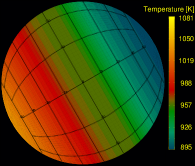
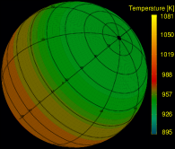
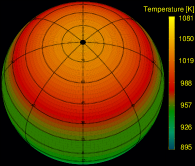
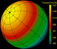
Figure 5: Temperature structure at the infrared photosphere, for the $\psi=60$° model, at $t/P_{\mathrm{orb}}=0$, $1/8$, $2/8$, and $3/8$ (from left to right). In each plot the axis is oriented to the perspective of an observer who would see the planet go into secondary eclipse at that time, assuming that the angular momentum vector of the orbit is pointed up on the page.

There are two important degeneracies that influence the orientation of the brightness structure that can be measured by eclipse mapping: the unknown North-South orbital orientation of the system, and a seasonal hemispheric degeneracy. Figure 6 shows schematic examples of these degeneracies. Since we are not spatially resolving the planet from the star, but rather using the time domain to separate out its signal, we do not know the orientations of the orbital or rotational angular momentum vectors relative to us, the latter of which defines which hemisphere is the Northern one. We may be able to determine that one hemisphere is hotter than the other, but cannot label it as “North” or “South”. This degeneracy was also discussed above in Section 4.1, as it relates to the phase curves only being sensitive to the absolute value of the subobserver latitude.

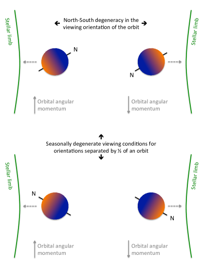
Figure 6: A diagram of the degeneracies that result from the unknown viewing orientation of the system. As distant observers, we cannot tell which hemisphere is the planet’s North or South, nor can we tell Northern summer from Southern summer.

The second degeneracy diagrammed in Figure 6 is a physical degeneracy in the seasonal response between the two hemispheres. There are no sources of North-South asymmetry for our idealized hypothetical planet and so we see identically changing heating and cooling patterns in each hemisphere’s temperature structure. This explains why times separated by one half of an orbit have mirror-imaged temperature patterns. Since the North-South viewing degeneracy also exists, this means that we cannot discriminate between these seasonally identical conditions. For the example diagrammed in Figure 6, we cannot differentiate between a planet that is passing into eclipse in Northern winter or Northern summer, because in either case the hotter hemisphere will be eclipsed first. This degeneracy is also implicitly found in Figure 3, in that each curve is actually two overlapping predictions: the $+\phi_{\mathrm{obs}}$ and $-\phi_{\mathrm{obs}}$ solutions with times separated by half an orbit.

Even with those degeneracies, there still are several important pieces of information that we can measure with eclipse mapping. We calculate these from each of our models and plot them in Figure 7:

1. On the vertical axis we plot the secondary eclipse depth, or disk-integrated flux emitted from the hemisphere facing the observer.

2. The color of each point shows the amplitude of the flux gradient, meaning the difference in flux between the brightest and dimmest regions of the planet, for the observed hemisphere.

3. On the horizontal axis we plot the projected axial tilt, meaning the orientation of the flux gradient relative to the direction of the motion of the stellar limb. Specifically, we calculate the projected angle of the observed flux gradient and take the difference between this an the planet’s orbital angular momentum (which is perpendicular to the direction of motion of the stellar limb). Due to the degeneracies discussed above and diagrammed in Figure 6, we only calculate the absolute value of this tilt (i.e., not whether it is tipped clockwise or counterclockwise) and only characterize it with values $\leq 90\arcdeg$ (i.e., do not differentiate between the Northern or Southern hemisphere).

The third property listed, the projected tilt of the flux gradient, is the mostly directly observable indication of the planet’s obliquity. This is because our axisymmetric models always have flux gradients aligned with the rotation axis and so we are effectively measuring the projected obliquity. This will, however, be a function of the (arbitrary) viewing orientation of the seasons relative to our line-of-sight and so may take on a range of values. Results for each of our obliquity models (plotted using different symbols) were calculated at evenly spaced snapshots in time throughout the planet’s orbit, in order to explore the possible range of observed properties. In Figure 7 we also choose several representative datapoints for the different obliquity models and show the planet flux map that corresponds to each of those cases.

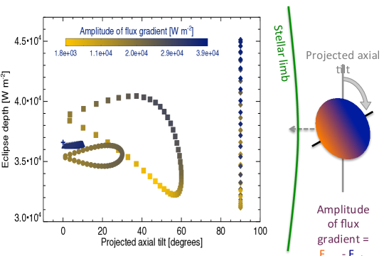
Figure 7: The properties of a planet measurable by eclipse mapping: the total flux from the observed hemisphere of the planet (eclipse depth), the gradient in flux across the planet disk (amplitude in color), and the orientation of the planet’s axis relative to the stellar limb, assuming the rotation is aligned with the flux gradient (projected axial tilt). Each point corresponds to the properties of a map that could be measured for models with obliquity equal to 0° (cross), 10° (triangles), 30° (circles), 60° (squares), and 90° (diamonds), depending on the orientation of the observer relative to the planet’s orbit. Also shown are the flux maps corresponding to several representative datapoints, oriented as they would be observed in secondary eclipse, with the stellar limb moving horizontally across the page. The color gradient for these maps is the same as in Figure 4 (white/yellow is the brightest, red is dimmer) and all maps share the same scale so that they can be directly compared to each other.

The zero obliquity model has no seasonal variation and its temperature structure remains unchanging throughout the year. Its eclipse depth, flux gradient, and projected axial tilt will always be the same value, independent of viewing orientation. These values are all nearly degenerate with the results for the $\psi=10\arcdeg$ model, whose temperature structure is very similar and shows only minimal seasonal variation. The only slight difference is that the project tilt for this model could be observed as anything between 0° and 10°, depending on the orientation of the observer relative to the seasonal cycle. It is unlikely that observations could discriminate between these low obliquity cases for our hypothetical planet.

When we compare the predicted eclipse mapping data for models with higher obliquities and stronger seasonal variation, we do see observable differences. There are some times during its orbit when the $\psi=90\arcdeg$ model would be observed to have the same eclipse depth and flux gradient amplitude as the $\psi=0\arcdeg$ model, but its projected axial tilt is always at 90° (always aligned with the direction of motion of the stellar limb and so perpendicular to the orbital angular momentum); this would be a clear way to discriminate between these two extremes in obliquity.

Another piece of information from eclipse mapping that would help to differentiate between planets with obliquities of 0° or 90° is that the flux gradient for the 0° case is peaked at the equator and drops off toward the poles, while the 90° case has a North-South gradient that stretches across the whole planet. This type of spatial information is retrieved in eclipse mapping observations, although we have not quantified it in our analysis here. Nevertheless, it is worth emphasizing that the planets with equators hotter than their poles (our $\psi=$0°, 10°, and 30° models) should be observed to have a different pattern of emission than planets where one hemisphere is hotter and brighter than the other (our $\psi=$60° or 90° models). However, this will depend some on the viewing orientation; for example, a high-latitude viewing orientation for a planet with a hotter equator and cooler poles could perhaps mimic the hemispheric flux difference of a higher obliquity planet, depending on the level of detail that can be retrieved with eclipse mapping.

Our models with obliquities of 30° and 60° show intermediate eclipse-mapping properties in Figure 7. They both have possible projected axial tilt values from zero up to their full obliquities, but observing a non-zero tilt only constrains the possible obliquities to be greater than or equal to that value. However, here we can see eclipse mapping’s power to constrain a planet’s obliquity. While models with different obliquities could produce the same the same projected axial tilt, the same eclipse depth, and/or the same flux gradient amplitude, these properties can generally be used in combination to break degeneracies between the different possible planet obliquities. In the next Section we estimate the ability of current and future instrumentation to perform precise enough measurements to be able to constrain a warm Jupiter’s obliquity.

4.3 Current and future instrument sensitivity

We have predicted two types of observations that could potentially be used to discern a planet’s obliquity: orbital phase curves and eclipse maps. Here we compare the signals predicted by our models to the instrumental sensitivity of current and future missions. We use rough estimates, since our modeled planet is hypothetical and we have to wait for a specific system to be targeted before more detailed estimates can be made. First we go through the exercise of estimating signal-to-noise assuming that the planet orbits a bright star and that we can achieve photon-limited precision, before a discussion of how to scale to less optimistic circumstances.

4.3.1 Predicted planet-to-star flux ratio

We already have predictions for the flux emitted from the planet, as a function of obliquity and viewing orientation (Figures 3 and 7), but the actual observable is the planet-to-star flux ratio, which we estimate as follows. The double-gray radiative transfer scheme used in our circulation model separates the optical absorbed stellar light from the thermally re-emitted infrared light, with the result that the predicted emission shown above is a general “infrared” emission and in fact encompasses all emission from the planet (for details, see Rauscher & Menou, 2012). If we view this in a bolometric sense, then the planet-to-star flux ratio is $\sim 6\times 10^{-4}$, based on an average planetary emission of $\sim 3.6\times 10^{4}$ W m^-2 (from Figures 3 and 7) and assuming Sun-like properties of the host star.

In comparing our predictions to specific instruments, it is important to consider the strong wavelength dependence of the planet-to-star flux ratio. Assuming Planck functions for the planetary and stellar emission, their flux ratio at some wavelength can be calculated as: $(R_{p}/R_{s})^{2}\times B(\lambda,T_{p})/B(\lambda,T_{s})$. Using the planet’s equilibrium temperature of $\sim$880 K, which is close to the average temperature at the planet’s infrared photosphere (Figure 2), we can estimate the planet-to-star flux ratio for Hubble (WFC3 G141, 1.4 micron) as $\sim 4\times 10^{-7}$ and for Spitzer (IRAC1, 3.6 micron) or JWST (NIRCam F356W, 3.5 micron) as $\sim 1\times 10^{-4}$.

4.3.2 Estimates of precision

We base our precision estimates on the values from Table 3 of Cowan et al. (2015), which assume the photon-counting limit for a target 20 pc away around a 5000 K host star. We adjust these predictions from an assumed integration time of 1 hour to the $\sim$4 hour length of the secondary eclipse for our hypothetical planet ($=2R_{s}/[2\pi a/P_{\mathrm{orb}}]$). Since our various measurements are all differential (in- vs. out-of-eclipse, amplitude at one phase vs. another) and so require the comparison of two different flux-level measurements, we apply a $\sqrt{2}$ penalty and obtain optimistic precisions of 1.6 ppm, 11 ppm, and 1.6 ppm (parts per million) for Hubble (WFC3 G141), Spitzer (IRAC1), and JWST (NIRCam F356W), respectively. We can only make educated guesses as to JWST’s actual performance until it begins operations, but based on lab tests of its detectors (noise floor estimates, quantum efficiencies, etc.), as well as previous experience with Hubble and Spitzer, we expect that JWST will achieve excellent photometric precision for exoplanet transits and eclipses (Beichman et al., 2014).

4.3.3 Detection of secondary eclipse

The largest, easiest signal to detect is that of the secondary eclipse of the planet. Using the planet-to-star flux ratios and precisions estimated in the previous two sections, we expect that with a single observation (assuming photon-limited precision) the secondary eclipse of our hypothetical warm Jupiter would not be detected by Hubble, but could have been detected by Spitzer at 9-$\sigma$, and should be detectable by JWST at 80-$\sigma$.

This optimistic prediction implies that JWST should be able to measure the eclipse depths plotted in Figure 7 to a precision of $\sim 0.2\times 10^{4}$ W m^-2 at 3-$\sigma$. The eclipse depths of the models with $\psi=0\arcdeg$ and 10° will be indistinguishable, the lowest possible values of the $\psi=30$°  model may be barely distinguishable from the lower obliquity cases, and much of the range of values for the $\psi=60$° or 90° models should be easily distinguishable. Since these are single-eclipse estimates, we could further improve the precision by collecting multiple observations, since we see no significant orbit-to-orbit variability on the planet.

4.3.4 Detection of variation in orbital phase

According to Figure 3, the amplitude of orbital flux variation we should observe depends both on the planet’s obliquity and our viewing orientation, with the (a priori unknown) viewing orientation having a strong influence on the phases of maximum and minimum flux. Since the orbital period is 10 days, it would be observationally very expensive to monitor a continuous, full orbit of the system and so a few shorter integration observations would probably be preferred (Krick et al., 2016). If there was already a secondary eclipse observation, that would help to constrain possible combinations of obliquity and viewing orientation, and help to intelligently schedule snapshots throughout the orbit.

We will side-step the issue of timing and instead just assume that there is one 4-hour observation near the peak in flux and one 4-hour observation near the minimum, in order to determine what level of variation could be measured. From our estimates of signal and precision, we determined above that JWST should be able to measure flux differences of $\sim 0.2\times 10^{4}$ W m^-2 for this planet at 3-$\sigma$. This means that all of the phase curves for equatorial viewing geometries (the solid lines in Figure 3) would be considered flat, as would the maximally variable curve for the $\psi=10$° model. All of the rest of the curves shown in Figure 3 (non-equatorially viewed models with $\psi\geq 30$°) would have measurable variation, at the 9- to 40-$\sigma$ level with JWST.

4.3.5 Detection of flux gradient via eclipse mapping

The detection of a gradient in flux across the planet’s disk can be measured during the ingress and egress times of secondary eclipse, given a high enough precision. This limits the integration time of the observation to the time that it takes the planet disk to move behind the star (or re-emerge), $2R_{p}/(2\pi a/P_{\mathrm{orb}})=0.4$ hours. Whereas for the eclipse depth measurement we assume an integration time of 4 hours and apply a $\sqrt{2}$ penalty for comparison with a baseline measured out of eclipse, here all of the information is contained within the times of ingress and egress. We thus use only 0.4 hours as the integration time, instead of 0.8 for the full ingress plus egress, and still apply the $\sqrt{2}$ penalty for a differential measurement. We could simplistically think of this as a comparison in flux between the first/second half of ingress/egress and the second/first half of ingress/egress. While the details of eclipse mapping are actually more complex (Williams et al., 2006; Rauscher et al., 2007; de Wit et al., 2012; Majeau et al., 2012), this method still relies on comparing the differential flux during some time(s) of ingress/egress to other times. This adjusts our predicted precision, assuming a single eclipse mapping observation with JWST, to 4 ppm.

The signal we are trying to measure in eclipse mapping is the difference in shape between an ingress/egress curve for a planet disk with uniform brightness and one with a flux gradient. If the gradient stretches across the globe, so that one hemisphere is above average and the other below, then we can simplistically assume that the maximum signal occurs when the planet is half-occulted by the star (in reality this depends on the projected angle of the gradient relative to the stellar limb). In this case, we apply a penalty of $1/2$ to the expected signal, since only half of the planet is in view. For planets with an equator-to-pole flux gradient, the same simplistic assumption would imply the greatest signal is when $1/4$ of the planet is occulted or left in-view. The ingress and egress signals would then average out to the same factor of $1/2$. The amplitude of the signal we are trying to measure is then roughly $(1/2)F_{\mathrm{grad}}/F_{*}$. (If the gradient is equal to the eclipse depth, then halfway through ingress/egress the flux would be $1/2\ F_{\mathrm{ed}}$ different from the flux of a uniformly bright disk; if there is no gradient the signal is zero.)

Note that one underlying assumption of our analysis is that our predicted JWST observations are at sufficient cadence to resolve the shape of the light curve during ingress and egress well enough to retrieve the spatial information. This is a safe assumption for two reasons. First, Spitzer has demonstrated sufficient cadence for mapping a similarly bright target (de Wit et al., 2012; Majeau et al., 2012), albeit with stacked observations, and the time-series imaging mode for NIRCam has been specifically designed for high-precision and high-cadence observations of bright sources, a significant improvement over Spitzer. Second, in the simplified estimate here we are effectively binning down to two points during ingress and two during egress, since we are only trying to estimate an amplitude for the flux gradient, rather than its spatial shape. As such, the observational cadence of JWST is not a concern here.

We can then take the planet-to-star flux ratios estimated above, multiply by $0.5F_{\mathrm{grad}}/F_{\mathrm{ed}}$, and divide by our estimated JWST precision for this type of measurement to determine the detectability of our predicted flux gradients. From the eclipse depths and flux gradients presented in Figure 7 we determine that the lower end of the $F_{\mathrm{grad}}/F_{\mathrm{ed}}$ range for the $\psi=60\arcdeg$ model is not accessible to eclipse mapping with a single observation, the lower end of that range for the $\psi=90\arcdeg$ model is marginally mappable (3-$\sigma$), and all other possible views of all other models could be mapped with a single JWST observation. The minimum for the $\psi=30\arcdeg$ model is 6-$\sigma$ and the maximum values for the $\psi=0$°, 10°, 30°, 60°, and 90° models are 13-$\sigma$, 12-$\sigma$, 9-$\sigma$, 9-$\sigma$, and 12-$\sigma$, respectively.

The technique of eclipse mapping has only successfully been applied to a single exoplanet (HD 189733b, de Wit et al., 2012; Majeau et al., 2012) and does not yet have a standardized method of analysis, making it difficult for us to predict the precision to which axial tilts could be measured. Both de Wit et al. (2012) and Majeau et al. (2012) presented multiple possible maps that could be reconstructed, depending on the particular form of equations used to describe the planet map. This motivates work such as Rauscher, Suri, & Cowan (in prep), in which we present orthonormal basis sets of maximally informative light curves and the corresponding “eigenmaps” that can be combined to reconstruct the planet map. However, our ability to accurately use the method of eclipse mapping is limited by the precision with which we know other properties of the system, namely the planet’s eccentricity, its impact parameter (or alternatively its orbital inclination), and the global density of the star (which influences the orbit of the planet), as demonstrated by de Wit et al. (2012). It is left to more detailed future work to precisely quantify the sensitivity of eclipse mapping measurements to both the amplitudes of flux gradients and their projected tilts.

4.3.6 A less optimistic signal-to-noise estimate

For the estimates in the sections above, we have optimistically assumed that JWST will be able to reach photon-limited precision and that our hypothetical planet orbits a nearby bright star. Here we briefly consider how our estimated signal-to-noise decreases if we make less generous assumptions. While none of these factors can actually be known before JWST is in operation, or before a warm Jupiter system to study is identified, it is possible to adjust our expectations for less desirable circumstances.

The hypothetical target star used by Cowan et al. (2015) to estimate instrument precision, which we use as a basis for our signal-to-noise estimate, has similar properties to the bright hot Jupiter host star HD 189733 ($d=19.45$ pc, $T_{\mathrm{eff}}=5040$ K), which has a $V$ magnitude of 7.7. The expected yield from the Transiting Exoplanet Survey Satellite (TESS) includes about 20 gaseous exoplanets (meaning radii larger than 4 Earth radii) with periods less than 20 days, orbiting stars with magnitudes as faint as $I_{C}\sim 12$, which is roughly the magnitude we would expect for the HD 189733-like host star used in the calculations above. So if we target a warm Jupiter from the TESS survey, we may expect our optimism about a bright host star to be fair. If, however, we are limited to the currently known warm Jupiter population (see the Introduction), then a host star $V$ magnitude of 10 would make our precision $\sim$3 times worse. This would still allow for most of our predicted flux gradients to be detected at greater than 3-$\sigma$ with a single JWST observation.

On the instrument side, while it may be overly optimistic to assume that JWST will reach photon-limited precision, the realized performance may not be too far off from it. Cowan et al. (2015) showed that their photon-limited precision estimates for HST and Spitzer were within a factor of 2 to 3 of the precisions actually achieved for exoplanet transits and eclipses. This is encouraging, especially since the NIRCam, NIRISS, and NIRSpec instruments will all use the same type of detector as HST. A factor of 2-3 worse precision is the same as our above consideration of a dimmer stellar host, meaning that we would still be able to measure most of the possible flux gradients to better than 3-$\sigma$.

We also have reason for some optimism in that, even if the precision of JWST is not as spectacular as one might hope, we should still be able to stack together multiple eclipses to achieve improved precision. The original eclipse mapping measurement was achieved by stacking together seven Spitzer eclipses (de Wit et al., 2012; Majeau et al., 2012). Even if the performance of JWST were an order of magnitude worse that photon-limited precision, stacking $\sim$4-9 eclipses would still allow us to measure the maximum flux gradients predicted for each obliquity model (and thus help to constrain a warm Jupiter’s obliquity) at 3-$\sigma$, although $\sim$25 eclipses would be needed to get these to 5-$\sigma$ detections.

5 Summary and conclusions

We have presented a set of three-dimensional atmospheric models for a hypothetical Jupiter-like planet on a 10-day period orbit around a Sun-like star, testing possible planetary obliquities ($\psi$) of: 0°, 10°, 30°, 60°, and 90°. We find that seasonal variations are negligible for $\psi\leq 10$° and important for $\psi\geq 30$°, to a level that should be measurable with the James Webb Space Telescope.

The circulation pattern of the $\psi\leq 30$° models is characterized by two high-latitude eastward jets (one in each hemisphere) and an equator that is hotter than the poles. For the $\psi=30$°  model the hot region near the equator shifts slightly up and down in latitude, as a delayed response to the seasonally shifting irradiation pattern. This atmospheric response time of $\sim$1/8 $P_{\mathrm{orb}}$, which is about an order of magnitude longer than the radiative timescale at the infrared photosphere, is also seen in the seasonal variations of the models with $\psi\geq 60$°. For those models the temperature pattern is characterized by one hemisphere being hotter during its summer and then a more uniform temperature distribution during equinoxes.

The observable features of each model depends not only on its obliquity, but also on the orientation with which the system is viewed, relative to the seasonal cycle. This results in observational degeneracies between inherent and coincidental properties; however, by combining multiple measurements, it may be possible to constrain a planet’s obliquity. From observing the light emitted by the planet as a function of orbital phase, we can determine:

• the efficiency of equator-to-pole heat transport, if the phase curve is flat and is at a level higher than the global average for re-emission of absorbed starlight,

• the obliquity of the planet, if the phase curve is flat and at a level below the global value for re-emitted starlight, or

• degenerate information about the planet’s obliquity, our viewing orientation, and the atmospheric seasonal response time, if the phase curve shows measurable variation.

Eclipse mapping, which resolves the dayside of the planet when it is eclipsed by the star, can provide more information than orbital phase curves and will require significantly less telescope time. We present quantitative predictions for the three main features measured by eclipse mapping: the total flux emitted from the observed hemisphere, the gradient in emitted flux across the hemisphere, and the orientation of that gradient relative to the direction of motion of the stellar limb. While none of these parameters can uniquely constrain the planet’s obliquity on its own, their combination can usually only match the predictions from a single obliquity model. The exceptions are the $\psi=0\arcdeg$ and 10° models, which have very similar values for each of these predicted observables. Thus eclipse mapping can either constrain a planet’s obliquity to be small (if $\leq 10\arcdeg$), or can measure it if significantly non-zero ($\geq 30\arcdeg$).

The phase curve and eclipse mapping methods are also complementarily informative. For example, independent of obliquity, the smallest phase curve variations occur for equatorial viewing geometries; but if we observe the system from this orientation, the projected axial tilt measured by eclipse mapping will be equal to the true obliquity of the planet. In this way, the multiple parameters that can be observed with eclipse mapping could be combined with phase curve measurements to provide even better constraints on the planet’s obliquity. If we first obtain the (observationally cheaper) eclipse map measurement, we could use the information contained there to identify which orbital phases might be the most informative (providing information about the atmospheric response time and/or efficiency of meridional heat transport) and sidestep the need for continuous observation (Krick et al., 2016).

Finally, we compare our various predicted signals to the sensitivity of current and future instruments. We find that Hubble observes at wavelengths too short to be useful for observing this hypothetical planet; however, the James Webb Space Telescope will be an amazing instrument for this type work. If we assume photon-limited precision and a host star as bright as HD 189733, then JWST should be able to detect the secondary eclipse of this hypothetical warm Jupiter at $\sim$80-$\sigma$ in a single observation, which is sensitive enough to eclipse-map the planet, measuring the hemispheric flux gradient and its orientation.

We have determined that the expected non-zero obliquities of warm Jupiters should both influence the observational characterization of these planets, and also be measurable with JWST. Future work will need to determine the observational degeneracies between the diversity of possible values we expect for the obliquities, eccentricities (Gaidos & Williams, 2004; Kataria et al., 2013), and rotation rates (Showman et al., 2015) of warm Jupiters. Since the obliquities (along with eccentricities and rotation rates) are presumably markers of the formation, evolution, and tidal processes that influence these planets, this adds an extra dimension of study for warm Jupiters, beyond the lessons we can learn from their bulk compositions (e.g. Thorngren et al., 2016).

References

- Anderson et al. (2014) Anderson, D. R., Collier Cameron, A., Delrez, L., et al. 2014, MNRAS, 445, 1114
- Beichman et al. (2014) Beichman, C., Benneke, B., Knutson, H., et al. 2014, PASP, 126, 1134
- Carter & Winn (2010) Carter, J. A., & Winn, J. N. 2010, ApJ, 709, 1219
- Charbonneau et al. (2002) Charbonneau, D., Brown, T. M., Noyes, R. W., & Gilliland, R. L. 2002, ApJ, 568, 377
- Cho & Polvani (1996) Cho, J. Y.-K., & Polvani, L. M. 1996, Physics of Fluids, 8, 1531
- Cowan et al. (2013) Cowan, N. B., Fuentes, P. A., & Haggard, H. M. 2013, MNRAS, 434, 2465
- Cowan et al. (2012) Cowan, N. B., Voigt, A., & Abbot, D. S. 2012, ApJ, 757, 80
- Cowan et al. (2015) Cowan, N. B., Greene, T., Angerhausen, D., et al. 2015, PASP, 127, 311
- de Kok et al. (2011) de Kok, R. J., Stam, D. M., & Karalidi, T. 2011, ApJ, 741, 59
- de Wit et al. (2012) de Wit, J., Gillon, M., Demory, B.-O., & Seager, S. 2012, A&A, 548, A128
- Ferreira et al. (2014) Ferreira, D., Marshall, J., O’Gorman, P. A., & Seager, S. 2014, Icarus, 243, 236
- Fortney et al. (2007) Fortney, J. J., Marley, M. S., & Barnes, J. W. 2007, ApJ, 659, 1661
- Fromang et al. (2016) Fromang, S., Leconte, J., & Heng, K. 2016, A&A, 591, A144
- Gaidos & Williams (2004) Gaidos, E., & Williams, D. M. 2004, New Astronomy, 10, 67
- Guillot (2010) Guillot, T. 2010, A&A, 520, A27+
- Guillot et al. (1996) Guillot, T., Burrows, A., Hubbard, W. B., Lunine, J. I., & Saumon, D. 1996, ApJ, 459, L35
- Heng et al. (2014) Heng, K., Mendonça, J. M., & Lee, J.-M. 2014, ApJS, 215, 4
- Heng et al. (2011) Heng, K., Menou, K., & Phillipps, P. J. 2011, MNRAS, 413, 2380
- Kataria et al. (2013) Kataria, T., Showman, A. P., Lewis, N. K., et al. 2013, ApJ, 767, 76
- Kawahara (2016) Kawahara, H. 2016, ApJ, 822, 112
- Kawahara & Fujii (2010) Kawahara, H., & Fujii, Y. 2010, ApJ, 720, 1333
- Krick et al. (2016) Krick, J. E., Ingalls, J., Carey, S., et al. 2016, ApJ, 824, 27
- Li & Goodman (2010) Li, J., & Goodman, J. 2010, ApJ, 725, 1146
- Linsenmeier et al. (2015) Linsenmeier, M., Pascale, S., & Lucarini, V. 2015, Planet. Space Sci., 105, 43
- Liou (1980) Liou, K. N. 1980, An introduction to atmospheric radiation.
- Majeau et al. (2012) Majeau, C., Agol, E., & Cowan, N. B. 2012, ApJ, 747, L20
- May & Rauscher (2016) May, E. M., & Rauscher, E. 2016, ApJ, 826, 225
- Mayne et al. (2014) Mayne, N. J., Baraffe, I., Acreman, D. M., et al. 2014, A&A, 561, A1
- Nikolov & Sainsbury-Martinez (2015) Nikolov, N., & Sainsbury-Martinez, F. 2015, ApJ, 808, 57
- Peale (1999) Peale, S. J. 1999, ARA&A, 37, 533
- Rauscher & Kempton (2014) Rauscher, E., & Kempton, E. M. R. 2014, ApJ, 790, 79
- Rauscher & Menou (2012) Rauscher, E., & Menou, K. 2012, ApJ, 750, 96
- Rauscher et al. (2007) Rauscher, E., Menou, K., Seager, S., et al. 2007, ApJ, 664, 1199
- Schwartz et al. (2016) Schwartz, J. C., Sekowski, C., Haggard, H. M., Pallé, E., & Cowan, N. B. 2016, MNRAS, 457, 926
- Seager & Hui (2002) Seager, S., & Hui, L. 2002, ApJ, 574, 1004
- Shields et al. (2016) Shields, A. L., Barnes, R., Agol, E., et al. 2016, Astrobiology, 16, 443
- Showman et al. (2010) Showman, A. P., Cho, J. Y.-K., & Menou, K. 2010, Atmospheric Circulation of Exoplanets, ed. Seager, S., 471–516
- Showman et al. (2015) Showman, A. P., Lewis, N. K., & Fortney, J. J. 2015, ApJ, 801, 95
- Spiegel et al. (2009) Spiegel, D. S., Silverio, K., & Burrows, A. 2009, ApJ, 699, 1487
- Thorngren et al. (2016) Thorngren, D. P., Fortney, J. J., Murray-Clay, R. A., & Lopez, E. D. 2016, ApJ, 831, 64
- Williams et al. (1996) Williams, D. M., Kasting, J. F., & Caldeira, K. 1996, in Circumstellar Habitable Zones, ed. L. R. Doyle, 43
- Williams & Pollard (2003) Williams, D. M., & Pollard, D. 2003, International Journal of Astrobiology, 2, 1
- Williams et al. (2006) Williams, P. K. G., Charbonneau, D., Cooper, C. S., Showman, A. P., & Fortney, J. J. 2006, ApJ, 649, 1020
- Winn & Fabrycky (2015) Winn, J. N., & Fabrycky, D. C. 2015, ARA&A, 53, 409
- Zhu et al. (2014) Zhu, W., Huang, C. X., Zhou, G., & Lin, D. N. C. 2014, ApJ, 796, 67