Learning to Draw Samples with Amortized Stein Variational Gradient Descent

Abstract

We propose a simple algorithm to train stochastic neural networks to draw samples from given target distributions for probabilistic inference. Our method is based on iteratively adjusting the neural network parameters so that the output changes along a Stein variational gradient direction (Liu & Wang, 2016) that maximally decreases the KL divergence with the target distribution. Our method works for any target distribution specified by their unnormalized density function, and can train any black-box architectures that are differentiable in terms of the parameters we want to adapt. We demonstrate our method with a number of applications, including variational autoencoder (VAE) with expressive encoders to model complex latent space structures, and hyper-parameter learning of MCMC samplers that allows Bayesian inference to adaptively improve itself when seeing more data.

1 INTRODUCTION

Modern machine learning increasingly relies on highly complex probabilistic models to reason about uncertainty. A key computational challenge is to develop efficient inference techniques to approximate, or draw samples from complex distributions. Currently, most inference methods, including MCMC and variational inference, are hand-designed by researchers or domain experts. This makes it difficult to fully optimize the choice of different methods and their parameters, and exploit the structures in the problems of interest in an automatic way. The hand-designed algorithm can also be inefficient when there is a need to perform fast inference repeatedly on a large number of different distributions with similar structures. This happens, for example, when we need to reason about a number of observed datasets in settings like online learning or personalized prediction, or need fast inference as inner loops for other algorithms such as learning latent variable models (such as variational autoencoder (Kingma & Welling, 2013)) or unnormalized distributions. Therefore, it is highly desirable to develop intelligent probabilistic inference systems that can adaptively improve their own performance to fully optimize the computational efficiency, and generalize to new tasks with similar structures. Developing such systems requires solving the following learning-to-sample problem:

Problem 1.

Given a distribution with density $p(z)$ on set $\mathcal{Z}$ and a simulator $z=f(\xi;~{}\eta)$, such as a neural network, which takes a parameter $\eta$ and a random seed $\xi$ drawn from $q_{0}$ and outputs a value $z$ in $\mathcal{Z}$, we want to find an optimal parameter $\eta$ so that the density of the random output $z=f(\xi;~{}\eta)$ with $\xi\sim q_{0}$ closely matches the target $p$.

Here, we assume that we do not know the analytical form of the simulator $f(\cdot)$ (which we call inference network), and we can only query it through the output value $f(\xi;~{}\eta)$ and derivative $\partial_{\eta}f(\xi;~{}\eta)$ for given $\eta$ and $\xi$. We also assume that the random seed distribution $q_{0}$ is unknown and we can only access it through the draws of the random input $\xi$; that is, $q_{0}$ can be arbitrarily complex, and can be discrete, continuous or hybrid.

Because of the above assumption, we cannot directly calculate the density $q_{\eta}(z)$ of the output variable $z=f(\xi;~{}\eta)$; this makes it difficult to solve Problem 1 using the typical variational inference (VI) methods. Recall that VI finds an optimal parameter $\eta$ to approximate the target $p$ with $q_{\eta}$, by minimizing the KL divergence:

$$\mathrm{KL}(q_{\eta}~{}||~{}p)=\mathbb{E}_{q_{\eta}}[\log(q_{\eta}/p)].$$ (1)

However equation (1) requires calculating the density $q_{\eta}(z)$ or its derivative, which is intractable by our assumption (and is called implicit models in Mohamed & Lakshminarayanan (2016)). This holds true even when Monte Carlo gradient estimates (Hoffman et al., 2013) and the reparametrization trick (Kingma & Welling, 2013) are applied.

This requirement of calculating $q_{\eta}(z)$ makes it difficult for practitioners to use variational inference in an automatic way, especially in domains where it is critical to use expressive inference networks to achieve good approximation quality. Methods that do not require to explicitly calculate $q_{\eta}(z)$, referred to as wild variational inference, or variational programming (Ranganath et al., 2016), can significantly simplify the design and expand the applications of VI methods, allowing practioners to focus more on choosing proposals that work best with their specific tasks.

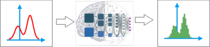
Figure 1: Wild variational inference allows us to train general stochastic neural inference networks to learn to draw (approximate) samples from the target distributions, without restriction on the computational tractability of the density function of the neural inference networks.

A similar problem also appears in importance sampling (IS), where it requires calculating the IS proposal density $q(z)$ in order to calculate the importance weight $w(z)=p(z)/q(z)$. However, there exist methods that use no explicit information of the proposal $q(z)$, and, seemingly counter-intuitively, give better asymptotic variance or converge rate than the typical IS that uses the proposal information (e.g., Liu & Lee, 2016; Briol et al., 2015; Henmi et al., 2007; Delyon & Portier, 2014). Discussions on this phenomenon date back to O’Hagan (1987), who argued that “Monte Carlo (that uses the proposal information) is fundamentally unsound”, and developed Bayesian Monte Carlo (O’Hagan, 1991) as an instance that uses no information of proposal $q(z)$, yet gives better convergence rate than the typical Monte Carlo $O(n^{-1/2})$ convergence rate (Briol et al., 2015). Despite the substantial difference between IS and VI, these results intuitively suggest the possibility of developing efficient variational inference without using the information of density function $q(z)$ explicitly.

Main Idea

In this work, we study a simple algorithm for Problem 1, motivated by a recent Stein variational gradient descent (SVGD) algorithm. Briefly speaking, SVGD is a nonparametric functional gradient descent algorithm which solves $\min_{q}\mathrm{KL}(q~{}||~{}p)$ without parametric assumption on $q$, and approximates the functional gradient, called the Stein variational gradient, using a set of samples (or particles) $\{z_{i}\}_{i=1}^{n}$ which iteratively evolves. See Section 2 for more introduction on SVGD. We can then view Problem 1 as a constrained optimization problem,

$$\min_{q}\mathrm{KL}(q~{}||~{}p),~{}~{}~{}~{}s.t.~{}~{}~{}q=q_{\eta}~{}~{}\text{for some $\eta$},$$ (2)

which motivates us to develop a project gradient like algorithm that iteratively calculates the Stein variational gradient, and projects it to the finite dimensional $\eta$-space to update parameter $\eta$. At the convergence, the samples drawn from $q_{\eta}$ reach the equilibrium state of SVGD, and hence form a good approximation of $p$. We can view this method as “amortizing” or distilling the SVGD dynamics using parametric family $q_{\eta}$ or its inference network $f(\xi;~{}\eta)$ and call it amortized SVGD. See Section 3 for the detailed description of amortized SVGD.

Our algorithm provides a simple approach for the wild inference problem in Problem 1, enabling wide application in approximate learning and inference. We explore two examples in this paper. In Section 4.1, we apply amortized SVGD to learn complex encoder functions in variational autoencoder (VAE), allowing it to model complex latent variable space. In Section 4.2 we use amortized SVGD to learn hyper-parameters of MCMC samplers, which allows us to adaptively improve the efficiency of Bayesian computation when performing a large number of similar tasks.

Related Work

There has been a number of very recent work that studies advanced variational inference methods that do not require explicitly calculating $q_{\eta}(z)$ (Problem 1). This includes adversarial variational Bayesian (Mescheder et al., 2017) which approximates the KL divergence with a density ratio estimator, operator variational inference (Ranganath et al., 2016) which replaces the KL divergence with an alternative operator variational objective that is equivalent to Stein discrepancy (see Appendix A for more discussion), and amortized MCMC (Li et al., 2017) which proposes to amortize arbitrary MCMC dynamics to make it applicable to discrete models and gradient-free settings.

The key advantage of our method is its simplicity. both Mescheder et al. (2017) and Ranganath et al. (2016) require training some type of auxiliary networks, while our main algorithm (Algorithm 1 with update (10)) is very simple, and is essentially a generalization of the typical gradient descent rule that replaces the typical gradient with the stein variational gradient.

It is also possible to adopt the auxiliary variational inference methods (e.g., Agakov & Barber, 2004; Salimans et al., 2015) to solve Problem 1 by treating $\xi$ as a hidden variable. however, in order to frame a tractable joint distribution $p(z,\xi)$, one would need to add additional noise on $z$, e.g., assume $z=f(\xi;~{}\eta)+\mathcal{N}(0,\sigma^{2})$ with a careful choice of noise variance $\sigma$, and also need to introduce an additional auxiliary network to approximate $q(\xi~{}|~{}z)$, which makes the algorithm more complex than ours.

The idea of amortized inference (Gershman & Goodman, 2014) has been recently applied in various domains of probabilistic reasoning, including both amortized variational inference (e.g., Kingma & Welling, 2013; Rezende & Mohamed, 2015) and date-driven designs of Monte Carlo based methods (e.g., Paige & Wood, 2016), to name only a few. Balan et al. (2015) also explored the idea of amortizing or distil MCMC samplers to obtain compact fast posterior representation. Most of these methods uses typical variational inference methods and hence need to use simple $q_{\eta}$ to ensure tractability.

There is a large literature on traditional adaptive MCMC methods (e.g., Andrieu & Thoms, 2008; Roberts & Rosenthal, 2009) which can be used to adaptively adjust the proposal distribution of MCMC by exploiting the special theoretical properties of MCMC (e.g., by minimizing the autocorrelation). Our method is simpler, more generic, and works efficiently in practice thanks to the use of gradient-based back-propagation. Finally, connections between stochastic gradient descent and variational inference have been discussed and exploited in Mandt et al. (2016); Maclaurin et al. (2015).

2 STEIN VARIATIONAL GRADIENT DESCENT

Stein variational gradient descent (SVGD) (Liu & Wang, 2016) is a nonparametric variational inference algorithm that iteratively transports a set of particles $\{z_{i}\}_{i=1}^{n}$ to approximate the target distribution $p$ by performing a type of functional gradient descent on the KL divergence. We give a quick overview of the SVGD in this section.

Let $p(z)$ be a positive density function on $\mathbb{R}^{d}$ which we want to approximate with a set of particles $\{z_{i}\}_{i=1}^{n}$. SVGD starts with a set of initial particles $\{z_{i}\}_{i=1}^{n}$, and updates the particles iteratively by

$$z_{i}\leftarrow z_{i}+\epsilon{\boldsymbol{\phi}}(z_{i}),~{}~{}~{}~{}\forall i=1,\ldots,n,$$ (3)

where $\epsilon$ is a step size, and ${\boldsymbol{\phi}}\colon\mathbb{R}^{d}\to\mathbb{R}^{d}$ is a velocity field which should be chosen to push the particle distribution closer to the target distribution. Assume the current particles are drawn from a distribution $q$, and let $q_{[\epsilon{\boldsymbol{\phi}}]}$ be the distribution of the updated particles $z^{\prime}=z+\epsilon{\boldsymbol{\phi}}(z)$ when $z\sim q$. The optimal choice of ${\boldsymbol{\phi}}$ can be framed as the following optimization problem:

$${\boldsymbol{\phi}}^{*}=\operatorname*{arg\,max}_{{\boldsymbol{\phi}}\in{\mathcal{F}}}\bigg{\{}-\frac{d}{d\epsilon}\mathrm{KL}(q_{[\epsilon{\boldsymbol{\phi}}]}~{}||~{}p)~{}\bigg{|}_{\epsilon=0}\bigg{\}},$$ (4)

that is, ${\boldsymbol{\phi}}$ should yield a maximum decreasing rate on the KL divergence between the particle distribution and the target distribution. Here, ${\mathcal{F}}$ is a function set that includes the possible velocity fields and is chosen to be the unit ball of a vector-valued reproducing kernel Hilbert space (RKHS) $\mathcal{H}=\mathcal{H}_{0}\times\cdots\times\mathcal{H}_{0}$, where $\mathcal{H}_{0}$ is a RKHS formed by scalar-valued functions associated with a positive definite kernel $k(z,z^{\prime})$, that is, ${\mathcal{F}}=\{{\boldsymbol{\phi}}\in\mathcal{H}\colon||{\boldsymbol{\phi}}||_{\mathcal{H}}\leq 1\}$. This choice of ${\mathcal{F}}$ allows us to consider velocity fields in infinite dimensional function spaces while still obtaining a closed form solution. Liu & Wang (2016) showed that the objective function in (4) equals a simple linear functional of ${\boldsymbol{\phi}}$:

$$~{}-\frac{d}{d\epsilon}\mathrm{KL}(q_{[\epsilon{\boldsymbol{\phi}}]}~{}||~{}p)\big{|}_{\epsilon=0}=\mathbb{E}_{x\sim q}[{\mathcal{T}}_{p}{\boldsymbol{\phi}}(x)],$$ (5)

$$~{}~{}\text{with}~{}~{}~{}{\mathcal{T}}_{p}{\boldsymbol{\phi}}(z)=\nabla_{x}\log p(z)^{\top}{\boldsymbol{\phi}}(z)+\nabla_{z}^{\top}{\boldsymbol{\phi}}(z),$$ (6)

where ${\mathcal{T}}_{p}$ is a linear operator acting on a velocity field ${\boldsymbol{\phi}}$ and returns a scalar-valued function; ${\mathcal{T}}_{p}$ is called the Stein operator in connection with Stein’s identity which shows that the RHS of (5) equals zero if $p=q$:

$$\mathbb{E}_{p}[{\mathcal{T}}_{p}{\boldsymbol{\phi}}]=\mathbb{E}_{p}[\nabla_{z}\log p^{\top}{\boldsymbol{\phi}}+\nabla_{z}\cdot{\boldsymbol{\phi}}]=0.$$ (7)

This is a result of integration by parts assuming the values of $p(z){\boldsymbol{\phi}}(z)$ vanish on the boundary of the integration domain. Therefore, the optimization in (4) reduces to

$$\!\!\!\!\mathbb{D}(q||p)\overset{def}{=}\max_{{\boldsymbol{\phi}}\in\mathcal{H}}\{\mathbb{E}_{z\sim q}[{\mathcal{T}}_{p}{\boldsymbol{\phi}}(z)]~{}~{}~{}s.t.~{}~{}~{}~{}||{\boldsymbol{\phi}}||_{\mathcal{H}}\leq 1\},$$ (8)

where $\mathbb{D}(q~{}||~{}p)$ is the kernelized Stein discrepancy defined in (Liu et al., 2016; Chwialkowski et al., 2016), which equals zero if and only if $p=q$ under proper conditions that ensure the function space $\mathcal{H}$ is rich enough.

Observe that (8) is “simple” in that it is a linear functional optimization on a unit ball of a Hilbert space. Therefore, it is not surprise to derive a closed form solution:

$${\boldsymbol{\phi}}^{*}(\cdot)\propto\mathbb{E}_{z\sim q}[\nabla_{z}\log p(z)k(z,\cdot)+\nabla_{x}k(z,\cdot)],$$ (9)

where $k(z,z^{\prime})$ is the positive definite kernel associated with RKHS $\mathcal{H}_{0}$. See Liu et al. (2016) for the derivation. We call ${\boldsymbol{\phi}}^{*}$ the Stein variational gradient direction since it provides the optimal direction for pushing the particles towards the target distribution $p$.

In the practical SVGD algorithm, we start with a set of initial particles, calculate its corresponding ${\boldsymbol{\phi}}^{*}$ by replacing the expectation under $q$ with the empirical average of particles, and use it to update the particles:

$$z_{i}~{}\leftarrow~{}z_{i}~{}+~{}\epsilon{\boldsymbol{\phi}}^{*}(z_{i}),~{}~{}~{}~{}~{}~{}~{}~{}\forall i=1,\ldots,n,$$ (10)

$${\boldsymbol{\phi}}^{*}(z_{i})=\frac{1}{n}\sum_{j=1}^{n}[\nabla_{z_{j}}\log p(z_{j})k(z_{j},z_{i})+\nabla_{z_{j}}k(z_{j},z_{i})].$$

The two terms in ${\boldsymbol{\phi}}^{*}(z_{i})$ play two different roles: the term with the gradient $\nabla_{z}\log p(z)$ drives the particles toward the high probability regions of $p(z)$, while the term with $\nabla_{z}k(z,z_{i})$ serves as a repulsive force to encourage different particles to be different from each other as shown in Liu & Wang (2016). Overall, this procedure provides diverse points for approximating distribution $p$ when it converges.

It is easy to see from (10) that ${\boldsymbol{\phi}}^{*}(z_{i})$ reduces to the typical gradient $\nabla_{z}\log p(z_{i})$ when there is only a single particle ($n=1$) and $\nabla_{z}k(z,z_{i})=0$ when $z=z_{i}$, in which case SVGD reduces to the standard gradient ascent for maximizing $\log p(z)$ (i.e., maximum a posteriori (MAP)).

Computing the Kernelized Stein Discrepancy

By substituting the ${\boldsymbol{\phi}}^{*}$ in (9) into (8), one can show that (Liu et al., 2016; Chwialkowski et al., 2016; Oates et al., 2017)

$${\mathbb{D}(q~{}||~{}p)}^{2}=\mathbb{E}_{z,z^{\prime}\sim~{}q}[\kappa_{p}(z,z^{\prime})],$$ (11)

where $\kappa_{p}(z,z^{\prime})$ is a positive definite kernel obtained by applying Stein operator on $k(z,z^{\prime})$ twice, as a function of $z$ and $z^{\prime}$, respectively. It has the following computationally tractable form:

$$\kappa_{p}(z,z^{\prime})= {\boldsymbol{s}}_{p}(z)^{\top}k(z,z^{\prime}){\boldsymbol{s}}_{p}(z^{\prime})+{\boldsymbol{s}}_{p}(z)^{\top}\nabla_{z^{\prime}}k(z,z^{\prime})$$

$$+\nabla_{z}k(z,z^{\prime})^{\top}{\boldsymbol{s}}_{p}(z^{\prime})+\nabla_{z}^{\top}(\nabla_{z^{\prime}}k(z,z^{\prime})),$$

where ${\boldsymbol{s}}_{p}(z)=\nabla_{z}\log p(z)$. The form of KSD in (11) provides a computationally tractable way for estimating the Stein discrepancy between a set of samples $\{z_{i}\}$ (e.g., drawn from an unknown $q$) and a distribution $p$ specified by its score function $\nabla_{z}\log p(z)$ (which is independent of its normalization constant),

$$\hat{\mathbb{D}}_{u}^{2}(\{z_{i}\}~{}||~{}p)=\frac{1}{n(n-1)}\sum_{i\neq j}[\kappa_{p}(z_{i},z_{j})],$$ (12)

where $\hat{\mathbb{D}}_{u}^{2}(q~{}||~{}p)$ provides an unbiased estimator (hence called a $U$-statistic) for $\mathbb{D}^{2}(q~{}||~{}p)$. As a side result of this work, we will discuss the possibility of using KSD as an objective function for wild variational inference in Appendix A.

Algorithm 1 Amortized SVGD for Problem 1

  Set batch size $m$, step-size scheme $\{\epsilon_{t}\}$ and kernel $k(z,z^{\prime})$. Initialize $\eta^{0}$.

  for iteration $t$ do

     Draw random $\{\xi_{i}\}_{i=1}^{m}$, calculate $z_{i}=f(\eta^{t};~{}\xi_{i})$, and the Stein variational gradient ${\boldsymbol{\phi}}^{*}(z_{i})$ in (10).

     Update parameter $\eta$ using either (13), (14) or (15).

  end for

3 AMORTIZED SVGD: TOWARDS AN AUTOMATIC NEURAL SAMPLER

SVGD and other particle-based methods become inefficient when we need to apply them repeatedly on a large number of different, but similar target distributions for multiple tasks, because they can not leverage the similarity between the different distributions and may require a large memory to restore a large number of particles. This problem can be addressed by training a neural network $f(\xi;~{}\eta)$ to output particles that would have been produced by SVGD; this amounts to “amortizing” or compressing the nonparametric SVGD into a parametric network, yielding a solution for wild variational inference in Problem 1 of Section 1.

One straightforward way to achieve this is to run SVGD until convergence and train $f(\xi;~{}\eta)$ to fit the resulting SVGD particles (e.g., by using generative adversarial networks (GAN) (Goodfellow et al., 2014)). This, however, requires running many epochs of fully converged SVGD and can be slow in practice. We instead propose an incremental approach in which $\eta$ is iteratively adjusted so that the network outputs $z=f(\xi;~{}\eta)$ improves by moving along the Stein variational gradient direction in (10), in order to move towards the target distribution.

Specifically, denote by $\eta^{t}$ the parameter estimated at the $t$-th iteration of our method; each iteration of our method draws a batch of random inputs $\{\xi_{i}\}_{i=1}^{m}$ and calculate their corresponding output $z_{i}=f(\xi_{i};~{}\eta^{t})$ based on $\eta^{t}$, where $m$ is a mini-batch size (e.g., $m=100$). The Stein variational gradient ${\boldsymbol{\phi}}^{*}(z_{i})$ in (10) would then ensure that $z^{\prime}_{i}=z_{i}+\epsilon{\boldsymbol{\phi}}^{*}(z_{i})$ forms a better approximation of the target distribution $p$. Therefore, we should adjust $\eta$ to make it output $\{z^{\prime}_{i}\}$ instead of $\{z_{i}\}$, that is, we want to update $\eta$ by

$$\eta^{t+1}\leftarrow \operatorname*{arg\,min}_{\eta}\sum_{i=1}^{m}||f(\xi_{i};~{}\eta)-z_{i}^{\prime}||_{2}^{2},$$ (13)

where $z_{i}^{\prime}=z_{i}+\epsilon{\boldsymbol{\phi}}^{*}(z_{i})$. This process is repeated until convergence, in which case the outputs of network $f$ can no longer be improved by SVGD and hence should form a good approximation of the target $p$. See Algorithm 1.

If we assume $\epsilon$ is very small, then (13) can be approximated by a least square optimization. To see this, note that $f(\xi_{i};~{}\eta)\approx f(\xi_{i};~{}\eta^{t})+\partial_{\eta}f(\xi_{i};~{}\eta^{t})(\eta-\eta^{t})$ by Taylor expansion. Since $z_{i}=f(\xi_{i};~{}\eta^{t})$, we have

$$||f(\xi_{i};~{}\eta)-z_{i}^{\prime}||_{2}^{2}\approx||\partial_{\eta}f(\xi_{i};~{}\eta^{t})(\eta-\eta^{t})-\epsilon{\boldsymbol{\phi}}^{*}(z_{i})||_{2}^{2}.$$

As a result, (13) reduces to a least square optimization:

$$\begin{split}&\eta^{t+1}\leftarrow\eta^{t}-\epsilon\Delta\eta^{t},\\ &\Delta\eta^{t}=\operatorname*{arg\,min}_{\delta}\sum_{i=1}^{m}||\partial_{\eta}f(\xi_{i};~{}\eta^{t})\delta-{\boldsymbol{\phi}}^{*}(z_{i})||_{2}^{2}.\end{split}$$ (14)

It may be still slow to solve a least square problem at each iteration. We can derive a more computationally efficient approximation by performing only one step of gradient descent of (13) starting at $\eta^{t}$ (or equivalently (14) starting at $\delta=0$), which gives

$$\eta^{t+1}\leftarrow\eta^{t}+\epsilon\sum_{i=1}^{m}\partial_{\eta}f(\xi_{i};~{}\eta^{t}){\boldsymbol{\phi}}^{*}(z_{i}).$$ (15)

Although update (15) is derived as an approximation of (13) or (14), it is computationally faster and it works effectively in practice; this is because when $\epsilon$ is small, one step of gradient update can be sufficiently close to the optimum.

Update (15) has a simple and intuitive interpretation: it can be thought as a “chain rule” that back-propagates the Stein variational gradient to the network parameter $\eta$. This can be justified by considering the special case when we use only a single particle $(n=1)$ in which case ${\boldsymbol{\phi}}^{*}(z_{i})$ in (10) reduces to the typical gradient $\nabla_{z}\log p(z_{i})$, and update (15) reduces to the typical gradient ascent for maximizing $\mathbb{E}_{\xi}[\log p(f(\xi;~{}\eta))],$ in which case $f(\xi;~{}\eta)$ is trained to maximize $\log p(z)$ (that is, learning to optimize), instead of learning to draw samples from $p$ for which it is crucial to use the Stein variational gradient ${\boldsymbol{\phi}}^{*}(z_{i})$ to diversify the outputs to capture the uncertainties in $p$.

Update (15) also has a close connection with the typical variational inference with the reparameterization trick (Kingma & Welling, 2013). Let $q_{\eta}(z)$ be the density function of $z=f(\xi;~{}\eta)$, $\xi\sim q_{0}$. Using the reparameterization trick, the gradient of $\mathrm{KL}(q_{\eta}~{}||~{}p)$ w.r.t. $\eta$ equals

$$\nabla_{\eta}\mathrm{KL}(q_{\eta}~{}||~{}p)=-\mathbb{E}_{\xi\sim q_{0}}[\partial_{\eta}f(\eta;~{}\xi)\nabla_{z}\log(p(z)/q_{\eta}(z))].$$

With $\{\xi_{i}\}$ i.i.d. drawn from $q_{0}$ and $z_{i}=f(\xi_{i};~{}\eta),~{}\forall i$, we can obtain a standard stochastic gradient descent for minimizing the KL divergence:

$$\begin{split}&\eta^{t+1}\leftarrow\eta^{t}+\sum_{i=1}^{m}\partial_{\eta}f(\xi_{i};~{}\eta^{t})\tilde{\boldsymbol{\phi}}^{*}(z_{i}),\\ \text{where}~{}~{}~{}~{}&\tilde{\boldsymbol{\phi}}^{*}(z_{i})=\nabla_{z}\log p(z_{i})-\nabla_{z}\log q_{\eta^{t}}(z_{i}).\end{split}$$ (16)

This is similar to (15), but replaces the Stein gradient ${\boldsymbol{\phi}}^{*}(z_{i})$ defined in (10) with $\tilde{\boldsymbol{\phi}}^{*}(z_{i})$. However, because $\tilde{\boldsymbol{\phi}}^{*}(z_{i})$ depends on the density $q_{\eta^{t}}$, which is assumed to be intractable in Problem 1, (16) is not directly applicable in our setting. Further insights can be obtained by noting that

$${\boldsymbol{\phi}}^{*}(z_{i}) \approx\mathbb{E}_{z\sim q_{\eta^{t}}}[\nabla_{z}\log p(z)k(z,z_{i})+\nabla_{z}k(z,z_{i})]$$

$$=\mathbb{E}_{z\sim q_{\eta^{t}}}[(\nabla_{z}\log p(z)-\nabla_{z}\log q_{\eta^{t}}(z))k(z,z_{i})]$$

$$=\mathbb{E}_{z\sim q_{\eta^{t}}}[\tilde{\boldsymbol{\phi}}^{*}(z)k(z,z_{i})],$$ (17)

where (3) is obtained by using Stein’s identity (7). Therefore, ${\boldsymbol{\phi}}^{*}(z_{i})$ can be treated as a smoothed version of $\tilde{\boldsymbol{\phi}}^{*}(z_{i})$ obtained by convolving it with kernel $k(z,z^{\prime})$.

4 APPLICATIONS OF AMORTIZED SVGD

With amortized SVGD, we can use expressive inference networks to obtain better approximation and explore new applications where traditional VI methods cannot be applied. In this section, we introduce two different applications of amortized SVGD. One is training variational autoencoders (Kingma & Welling, 2013) with complex, non-Gaussian encoders, and the other is training “smart” MCMC samplers that adaptively improve their own hyper-parameters from past experience.

4.1 Amortized SVGD For Variational Autoencoders

Variational autoencoders (VAEs) (Kingma & Welling, 2013) are latent variable models of form $p_{\theta}(x)=\int_{z}p_{\theta}(x|z)p_{\theta}(z)dz$ where $x$ is an observed variable and $z$ is an un-observed latent variable. Assume the empirical distribution of the observed variable is $\hat{p}(x)$, VAE learns the parameter $\theta$ using a variational EM algorithm which approximates the posterior distribution $p_{\theta}(z|x)$ with a simple encoder $q_{\eta}(z|x)$, and updates $\theta$ and $\eta$ alternatively by

$$\theta\leftarrow\operatorname*{arg\,max}_{\theta}~{}\mathbb{E}_{\hat{p}(x)q_{\eta}(z\mid x)}\big{[}\log p_{\theta}(x,~{}z)\big{]},$$ (18)

$$\eta\leftarrow\operatorname*{arg\,min}_{\eta}~{}\mathbb{E}_{\hat{p}(x)}\big{[}\mathrm{KL}(q_{\eta}(z\mid x)~{}||~{}p_{\theta}(z\mid x))\big{]},$$ (19)

which alternates between updating $\theta$ by maximizing the joint likelihood (M-step (18)) and approximating the posterior distribution $p_{\theta}(z|x)$ given fixed $\theta$ with variational inference (VI) (E-step (19)). In standard VAE, (18) is performed using standard VI with the reparameterization trick (16), which requires $q_{\eta}$ to be tractable. Therefore, $q_{\eta}(z\mid x)$ is often defined as a Gaussian distribution with mean and diagonal covariance parameterized by neural networks with $x$ as input. This Gaussian assumption potentially limits the quality of the resulting generative models, and more expressive encoders can improve the performance as shown in recent works (e.g, Kingma et al., 2016; Mescheder et al., 2017, to name a few).

By applying amortized SVGD to solve the posterior inference problem in (19), we obtain simple algorithms that work with more complex inference networks. Specifically, we assume that $z\sim q_{\eta}(z|x)$ is generated by $z=f(\xi,x;~{}\eta)$, and optimize $\eta$ using update (13)-(15). See Algorithm 2. In our experiment, we take $z=f(\xi,x;~{}\eta)$ to be a deep neural network with binary Bernoulli dropout noise at the input layer of the network which is more effective in approximating multi-modal posteriors than the simple Gaussian encoders.

Similar idea has also been explored in Pu et al. (2017). Besides, we propose an entropy regularized VAE to improve the standard VAE and get more diverse images by adding an entropy regularization term on the encoder networks. Here, we replace the $\eta$-update in (19) with

$$\eta \leftarrow\operatorname*{arg\,min}_{\eta}\mathbb{E}_{\hat{p}(x)}[\mathrm{KL}(q_{\eta}(z\mid x)~{}||~{}p_{\theta}(z\mid x))\big{]}-\alpha H(q_{\eta})$$

$$=\operatorname*{arg\,min}_{\eta}\mathbb{E}_{\hat{p}(x)}\big{[}\mathrm{KL}(q_{\eta}(z\mid x)~{}||~{}p_{\theta}(z\mid x)^{\frac{1}{1+\alpha}})\big{]},$$ (20)

where $H(q_{\eta})=-\mathbb{E}_{\hat{p}(x)q_{\eta}(z|x)}[\log q_{\eta}(z|x)]$ is the (conditional) entropy of $q_{\eta}(z|x)$, and $\alpha$ is a regularization coefficient. (20) can be solved by applying SVGD on the tempered distribution $p_{\theta}(z\mid x)^{\frac{1}{1+\alpha}}$, which can be done by $z_{i}~{}\leftarrow~{}z_{i}~{}+~{}\epsilon{\boldsymbol{\phi}}^{*}(z_{i})$ with

$$\begin{split}\!\!\!\!\!\!\!{\boldsymbol{\phi}}^{*}(z_{i})=\frac{1}{n}\sum_{j=1}^{n}[&\nabla_{z_{j}}\log p_{\theta}(z_{j}|x)k(z_{j},z_{i})~{}~{}+\\ &~{}~{}~{}~{}~{}~{}~{}~{}~{}~{}~{}~{}~{}~{}~{}~{}~{}+~{}~{}(1+\alpha)\nabla_{z_{j}}k(z_{j},z_{i})],\end{split}$$ (21)

where the temperature parameter $(1+\alpha)$ becomes a weight coefficient of the repulsive force; a high temperature (or equivalent a large entropy regularization) yields a strong repulsive force and push the particles to be further away from each other.

Algorithm 2 Amortized SVGD for training VAE

  Set batch size $m$ and kernel $k(z,z^{\prime})$.

  Initialize encoder parameter $\eta$ and decoder parameter $\theta$.

  for iteration $t$ do

     Pick input $x^{(i)}$ from the training data.

     Draw $\{\xi_{k}\}_{k=1}^{m}\sim q_{0}$, calculate $z_{k}^{(i)}=f(x^{(i)},\xi_{k};~{}\eta)\vspace{.1cm}$, and their Stein variational gradients ${\boldsymbol{\phi}}^{*}(z_{k}^{(i)})$ in (10) or (21) related to gradient $\nabla_{z}\log p_{\theta}(z_{k}^{(i)}|x^{(i)})$.

     Update $\eta$ using either (13), (14) or (15).

     Update $\theta$ with $~{}~{}~{}~{}~{}~{}~{}~{}~{}\theta\leftarrow\theta+\frac{1}{m}\sum_{k=1}^{m}\nabla_{\theta}\log p_{\theta}(x^{(i)},~{}z_{k}^{(i)})$.

  end for

4.2 Training Langevin Samplers

By viewing typical MCMC procedures as a simulator $f(\cdot)$, we can apply amortized SVGD to adaptively improve hyperparameters in MCMC inference. This is useful when we need to perform Bayesian inference on a large number of different, but similar datasets or posteriors, where we can adaptively improve the MCMC sampler for future tasks by leveraging the information of the previous tasks. An example of this, which we consider in this work, is adaptively learning optimal step sizes for Langevin dynamics.

To specify the general framework, we assume that we are interested in drawing samples from a set of distributions

$${\mathcal{Q}}=\{p_{\vartheta}(z)\colon\vartheta\in\Theta\},$$

indexed by parameter $\vartheta$. We are interested in learning a network $f(\xi,p_{\vartheta};~{}\eta)$ which maps the distribution $p_{\vartheta}$ to stochastic posterior samples. Note that this is a generalization of Problem 1 which focuses on approximating an individual distribution. In practice, $p_{\vartheta}$ could be the posterior distributions of unknown parameters of interest conditioning on different observed data, or models of different individuals in hierarchical models.

In order to learn the network $f(\xi,p_{\vartheta};~{}\eta)$, we modify Algorithm 1, to perform amortized SVGD on a randomly selected $p_{\vartheta}$ from ${\mathcal{Q}}$ at each iteration. See Algorithm 3. In this way, we expect that the trained network $f(\xi,p_{\vartheta};~{}\eta)$ can perform well on similar $p_{\vartheta}$ drawn from the same distribution, but never seen by the training algorithm.

A useful perspective is that typical MCMC methods can be viewed as neural networks $f(\xi,p_{\vartheta};~{}\eta)$ handcrafted by researchers, with nice theoretical properties. We can leverage the structure of existing MCMC to design the architecture of $f(\cdot)$, and use amortized SVGD to adaptively improve its parameters across different tasks.

As an example, Langevin dynamics draws samples from $p_{\vartheta}$ by starting with an initial sample $z^{0}$ and performing iterative random updates of form $z^{t+1}\leftarrow f_{t}(z^{t})$ with

$$f_{t}(z^{t})=z^{t}+\eta^{t}\odot\nabla_{z}\log p_{\vartheta}(z^{t})+\sqrt{2\eta^{t}}\odot\xi^{t},$$ (22)

which performs gradient ascent with a Gaussian perturbation. Here $\eta^{t}$ denotes a vector-valued step size at the $t$-th iteration and “$\odot$” denotes element-wise product, and $\xi^{t}$ is a standard Gaussian random vector of the same size as $z^{t}$.

Algorithm 3 Amortized SVGD for Learning to Sample a distribution family ${\mathcal{Q}}=\{p_{\vartheta}\colon\vartheta\in\Theta\}$

  Goal: Learn parameter $\eta$ to train $z=f(\xi,p_{\vartheta};~{}\eta)$ drawing samples from $p_{\vartheta}$.

  Set batch size $m$, and kernel $k(z,z^{\prime})$. Initialize $\eta^{0}$.

  for iteration $t$ do

     Randomly select $p_{\vartheta}$ from ${\mathcal{Q}}$.

     Draw random seed $\{\xi\}_{i=1}^{m}\sim q_{0}.$

     Calculate $z_{i}=f(\xi_{i},~{}p_{\vartheta};~{}\eta)$, and the Stein variational gradient ${\boldsymbol{\phi}}^{*}(z_{i})$ in (10).

     Update parameter $\eta$ using either (13), (14) or (15).

  end for

We can view $T$ iterations of Langevin dynamics as a $T$-layer neural network:

$$z^{T}=f(\xi,~{}p_{\vartheta};~{}\eta)=f_{T-1}\circ\cdots\circ f_{0}(\xi,~{}p_{\vartheta};~{}\eta),$$ (23)

in which the initial samples and the Gaussian noise form the random seeds of the network, that is, $\xi=\{\xi^{t}\}_{t=0}^{T-1}\cup\{z^{0}\}$, and the step sizes $\eta=\{\eta^{t}\}_{t=0}^{T-1}\vspace{0.1 cm}$ form the parameters which we can estimate using Algorithm 3. In cases when it is difficult to calculate $\nabla_{z}\log p_{\vartheta}$ exactly, such as the case of Bayesian inference with big datasets, we can use stochastic gradient Langevin dynamics (Welling & Teh, 2011) to approximate $\nabla_{z}\log p_{\vartheta}$ with subsampling, which introduces another source of randomness. This, however, does not influence the application of Algorithm 3, since our method does not need to know the structure of the random seed distribution.

In practice, a large value of $T$ would result in a deep network and cause a vanishing gradient problem. We address this problem by partitioning the $T$ layers into small blocks of size $5$ or $10$, and evaluate the gradient of the parameters in each block by back-propagating the Stein variational gradient from the output of its own block.

(a) Test Distribution (truth)	(b) Power Decay (15 steps)	(c) Power Decay (1,000 steps)	(d) Amortized SVGD (5 steps)	(e) Amortized SVGD (15 steps)

Figure 2: Learning to sample from GMM. We train Langevin samplers using amortized SVGD on a set of randomly generated GMMs, and evaluate the samplers on a new GMM shown in (a) generated randomly in the same way as the training GMMs, but unavailable in the training time. (d)-(e): The Langevin sampler with step size trained by amortized SVGD obtains close approximation with $T=5$ or $15$ steps. (b)-(c): The typical power decay step size requires more Langevin iterations (and hence computation cost) to converge.

Log10 MSE
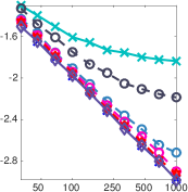
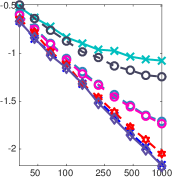
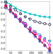
Sample Size ($n$)	Sample Size($n$)	Sample Size ($n$)
(a) $\mathbb{E}(x)$	(b) $\mathbb{E}(x^{2})$	(c) $\mathbb{E}(\cos(wx+b))$

Figure 3: Result on Gaussian-Bernoulli RBM. (a)-(c) show the mean square errors for estimating expectation $\mathbb{E}_{p}(h(x))$ using Langevin samplers with different numbers $T$ of steps, with either power decay step sizes or adaptive step size trained by amortized SVD. We take $h(x)=x^{j},(x^{j})^{2}$ and $\cos(wx^{j}+b)$ where $x^{j}$ denotes the $j$-th coordinate of vector $x$ and $w\sim\mathcal{N}(0,1)$ and $b\sim\mathrm{Uniform}(0,2\pi)$ and report the average MSE across all dimensions $j=1,\ldots,d$, over 20 random trials.

5 EXPERIMENTS

We apply amortized SVGD to the two different applications mentioned in section 4, and demonstrate that our method can train expressive inference networks to draw samples from intractable posterior distributions. For all our experiments, we use the standard RBF kernel $k(z,z^{\prime})=\exp(-\frac{1}{h}||z-z^{\prime}||^{2}_{2})$, and take the bandwidth to be $h=\mathrm{med}^{2}/\log n$, where $\mathrm{med}$ is the median of the pairwise distance between the current points $\{z_{i}\}^{n}_{i=1}$. We use update (15) in Algorithm 1, which solves Eq (13)-Eq (14) using a single gradient step. We find that using more gradient steps does not change the final results significantly, but may potentially increase the convergence speed (see Appendix B).

5.1 Training Langevin Samplers

In this section, we use amortized SVGD (Algorithm 3) to learn the step size parameters in the Langevin sampler in (23). We test a number of distribution families, including Gaussian Mixture, Gaussian Bernoulli RBM, Bayesian logistic regression and Bayesian neural networks. In all the cases, we train the sampler with a set of “training distributions” and evaluate the sampler on “test distributions” that are not seen by the algorithm during training. We compare our method to the typical Langevin sampler with power decay step size, selected to be the best from $\eta^{t}=10^{a}/(t+b)^{\gamma}$ where $\gamma=0.55$, $a\in\{-6,...,2\}$, $b\in\{0,...,9\}$.

Gaussian Mixture

We first train the Langevin samplers to learn to sample from simple Gaussian mixtures. We consider a family of Gaussian Mixtures $q_{\vartheta}(z)=\frac{1}{10}\sum_{i=1}^{10}\mathcal{N}(z;\vartheta_{i},0.1^{2})$, where $\vartheta$ is the mean parameter.

We train the sampler by drawing random elements of $\vartheta$ from $\mathrm{Uniform}(-1,1)$ at each iteration of Algorithm 3, and evaluate the quality of the samplers on new values of $\vartheta$ drawn from the same distribution, but not seen during training. In Figure 2, we find that the sampler trained by amortized SVGD obtains good approximation with $T=5$ or $15$ steps of Langevin updates (Figure 2(d)-(e)). In comparison, the typical Langevin sampler with the best power decay step size performs much worse (Figure 2(b)).

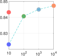
Test Accuracy	Test Accuracy
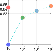
Steps of Langevin updates	Steps of Langevin updates
(a) Bayesian logistic regression	(b) Bayesian neural networks

Figure 4: By training the step size using amortized SVGD on dataset a9a, we obtain good performance “on” datasets a1a-a8a using Langevin sampler with only $T=10$ steps of Langevin updates.

Restricted Boltzmann Machine (RBM)

We test our method on Gaussian-Bernoulli RBM which is high dimensional and multi-modal. Gaussian-Bernoulli RBM is a hidden variable model consisting of a continuous observable variable $z\in\mathbb{R}^{d}$ and a binary hidden variable $h\in\{\pm 1\}^{\ell}$ with joint probability $p_{\vartheta}(z,h)\propto\exp(z^{\top}Bh+b^{\top}z+c^{\top}h-\frac{1}{2}||z||_{2}^{2}),$ where the parameters include $\vartheta=\{B,b,c\}.$ We obtain the marginal distribution of $p_{\vartheta}(z)$ by summing over $h$: $p_{\vartheta}(z)\propto\exp\big{[}b^{\top}z-\frac{1}{2}||z||_{2}^{2}+\sigma(B^{\top}z+c)\big{]},$ where $\sigma(h)=\sum_{i=1}^{\ell}\log(\exp(h_{i})+\exp(-h_{i}))$. In our experiments, we take $\ell=10$ hidden variables and $d=100$ observable variables, and randomly draw $b$ and $c$ from $\mathcal{N}(0,I)$ and $B$ uniformly from $\{\pm 0.1\}$ in the training time. The evaluation is on a new set of parameters $\vartheta=\{B,b,c\}$ drawn from the same distribution.

Figure 3 shows the result when we use the trained samplers to estimate integral quantities of form $\mathbb{E}_{p_{\vartheta}}[h]$ with different testing functions $h$. The plots show the MSE for estimating $\mathbb{E}_{p_{\vartheta}}[h]$ using $\sum_{i}h(z_{i})/n$ with $z_{i}$ generated from the trained sampler $z_{i}=f(\xi_{i},p_{\vartheta};~{}\eta)$. Here the sample size $n$ is the number of i.i.d. samples generated from the trained sampler in the testing time. In the case of typical, non-adaptive Langevin samplers, it is the number of Langevin Markov chains that we run in parallel. In Figure 3 (a)-(c), we generally find that amortized SVGD allows us to train high quality Langevin samplers with a small number $T$ of Langevin update steps. We observe that we can always further refine the result of our trained samplers using additional typical MCMC steps. For example, in Figure 3, we find that when using 20 steps of typical Langevin dynamics (with a power decay step size) to refine the output of the $T=30$ layer Langevin sampler trained by amortized SVGD achieves results close to the exact Monte Carlo.

Bayesian Classification

We test our method on Bayesian Logistic Regression and Bayesian neural networks for binary classification on real world datasets. In this case, the distribution of interest has a form of $p_{\vartheta}(z)=p(z|D)$, where $z$ is the network weights in logistic regression and neural networks, and $D$ is the dataset for binary classification, which we view as the parameter $\vartheta$, that is, different dataset $D$ yields different posterior $p(z|D)$, and we are interested in training the Langevin sampler on a set of available datasets, and hope it performs well on future datasets that have similar structures. This setting can be useful, for example, in the streaming setting where we use existing datasets to adaptively improve the Langevin sampler. In our experiment, we take nine similar datasets (a1a-a9) from the libsvm repository; we train our Langevin sampler on a9a, and evaluate the sampler on the remaining 8 datasets (a1a-a8a). Our training and evaluation steps are as follows:

1. Estimate the step sizes $\{\eta^{t}\}_{t=0}^{T-1}$ of the Langevin sampler using amortized SVGD based on dataset a9a.

2. Apply the Langevin sampler with the estimated step size to the training subsets of a$k$a, $k=1,\ldots,8$, to obtain posterior samples $\{z_{i}^{k}\}$ of the classification weights.

3. Calculate the test likelihood of $\{z_{i}^{k}\}$ on the testing subsets of a$k$a, $k=1,\ldots,8$. Report the averaged testing likelihood averaged on the 8 datasets in Figure 4.

Because each dataset is relatively large, we use the stochastic gradient approximation as suggested by Welling & Teh (2011) (with a minibatch size of 100) in Langevin samplers. We find that the $T=10$ Langevin samplers trained by amortized SVGD on a9a is comparable with the $T=10^{3}$ Langevin sampler with the best power decay step size.

5.2 Training VAE With Amortized SVGD

We compare the entropy regularized VAE trained with amortized SVGD (denoted by ESteinVAE), which is Algorithm 2 with update (21), with the standard VAE and entropy regularized standard VAE (denoted by EVAE) on the dynamically binarized MNIST dataset (Burda et al., 2015). We tested the following settings:

1. A standard VAE (VAE-f) with a fully connected encoder consisting of one hidden layer with 400 hidden units, and a Gaussian output hidden variable with diagonal covariance.

2. A standard convolutional Gaussian VAE (VAE-CNN) with a convolutional encoder consisting of 2 convolution layers with $5\times 5$ filters, stride 2 and $[16,32]$ features maps, followed by a fully connected layer with 512 hidden units.

3. A convolutional Gaussian entropy regularized (EVAE-CNN) with the same encoder and decoder structures as the standard convolutional VAE (VAE-CNN).

4. Entropy regularized VAEs trained by our amortized SVGD in Algorithm 2, with the same encoder architecture as VAE-f and VAE-CNN, respectively, but removing the Gaussian noise on the top layer and adding a multiplicative Bernoulli noise with a dropout rate of 0.3 to the each layer of the encoder. These two cases are denoted by ESteinVAE-f, and ESteinVAE-CNN, respectively.

In all these cases, we use $\mathrm{dim}(z)=32$ latent variables and the decoders have symmetric architectures as the encoders in all models. Adam is used with a learning rate tuned on the training images. For each training iteration, a batch of 128 images is used, and for each image we draw a batch of $m=5$ samples to apply amortized SVGD.

Marginal likelihood

Table 1 reports the test log-likelihood of all the methods estimated using Hamiltonian annealed importance sampling (HAIS) (Wu et al., 2016) with 100 independent AIS chains and 10,000 intermediate transitions, averaged on 5000 test images. We find that ESteinVAE-f significantly outperforms VAE-f, and ESteinVAE-CNN slightly outperforms VAE-CNN and EVAE-CNN. Table 1 also reports the effective sample size (ESS) of the HAIS estimates. The fact that the effective sample sizes of all the methods are close suggests that accuracy of the different NLL estimates are comparable.

Table 1: Negative log-likelihood on binarized mnist test dataset.

Model	NLL/nats	ESS
VAE-f	90.32	84.11
ESteinVAE-f	88.85	83.49
VAE-CNN	84.68	85.50
EVAE-CNN	84.43	84.91
ESteinVAE-CNN	84.31	86.57

Table 2: Quantitative imputation experiment based on 2,000 true images and 500 reconstructed images per true image.

Model	Accuracy	Entropy
ESteinVAE-CNN	0.84	0.501
EVAE-CNN	0.82	0.382
VAE-CNN	0.83	0.340

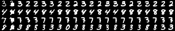
ESteinVAE-CNN

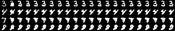
EVAE-CNN

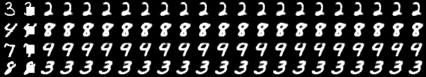
VAE-CNN

Figure 5: Imputation results from benchmark VAE-CNN, EVAE and ESteinVAE-CNN. The first column shows the original image. Col. 2 shows the missing image. The remaining columns show imputations for 20 reconstructed samples.

Missing data imputation

We demonstrate that ESteinVAE is able to learn multi-modal latent representation with the binary dropout noise. We consider missing data imputation with pixel missing in a square sub-regions of the image (the second column of Figure 5). We use a simple method to reconstruct image by applying one step of encode-decode operation starting from uniform noise $\mathrm{Uniform}(0,1)$. Specifically, let $x=[x^{v},x^{m}]$ where $x^{v}$ and $x^{m}$ denotes the visible and missing parts, respectively. Our imputation procedure consists of the following steps:

1. Draw $x^{c}$ from $\mathrm{Uniform}(0,1)$;

2. Draw $z\sim q_{\phi}(z|x^{c},~{}x^{v})$;

3. Draw $x\sim p(x|z)$.

Each column (starting from the third column) of Figure 5 shows an independent run of this procedure, where we can see that ESteinVAE-CNN is able to generate diverse construction when ambiguity exists, while the EVAE-CNN and VAE-CNN tend to be trapped in a local mode. This suggests that the diagonal variance of the latent variables in the Gaussian encoder of VAE-CNN tends to be small, underestimating the posterior uncertain, while ESteinVAE can capture the multi-modal posterior due to the dropout noise.

Table 2 is the quantitative result of the imputation experiment, in which the “accuracy” column denotes the number of original images whose digit is in its reconstructed images. and the “entropy” column denotes the entropy of the probability of the reconstructed images belonging to different digit classes. EsteinVAE obtains more diverse images and slightly more accurate reconstructed images.

6 CONCLUSION

We propose a new method to train neural samplers for given distributions, together with various applications to learning to draw samples using neural samplers. Future directions include exploring more efficient neural architectures and theoretical understanding of our method.

Acknowledgments
This work is supported in part by NSF CRII 1565796. We thank Yingzhen Li from University of Cambridge for her valuable comments and feedbacks.

Appendix A KSD Variational Inference

Kernelized Stein discrepancy (KSD) provides a discrepancy measure between distributions and can be in principle used as a variational objective function in replace of KL divergence. In fact, thanks to the special form of KSD ((11)-(12)), one can derive a standard stochastic gradient descent for minimizing KSD without needing to estimate $q_{\eta}(z)$ explicitly, which provides a conceptually simple wild variational inference algorithm. Although this work mainly focuses on amortized SVGD which we find to be easier to implement and tend to perform superior to KSD variational inference in practice (see Figure 6), we think the KSD approach is of theoretical interest and hence give a brief discussion here.

Specifically, take $q_{\eta}$ to be the density of the random output $z=f(\xi;~{}\eta)$ when $\xi\sim q_{0}$, and we want to find $\eta$ to minimize $\mathbb{D}(q_{\eta}~{}||~{}p)$. Assuming $\{\xi_{i}\}$ is i.i.d. drawn from $q_{0}$, we can approximate $\mathbb{D}^{2}(q_{\eta}~{}||~{}p)$ unbiasedly using the U-statistics in (12), and derive a standard gradient descent

$$\eta\leftarrow\eta-\epsilon\frac{2}{n(n-1)}\sum_{i\neq j}\partial_{\eta}f(\xi_{i};~{}\eta)~{}\nabla_{z_{i}}\kappa_{p}(z_{i},z_{j}),$$ (24)

where $z_{i}=f(\xi_{i};~{}\eta)$. This enables a wild variational inference method based on directly minimizing $\eta$ with standard (stochastic) gradient descent. We call this algorithm amortized KSD. Note that (24) is similar to (15) in form, but replaces ${\boldsymbol{\phi}}^{*}(z_{i})$ with

$$\bar{{\boldsymbol{\phi}}}^{*}(z_{i})\overset{def}{=}-2\sum_{j\colon i\neq j}\nabla_{z_{i}}\kappa_{p}(z_{i},z_{j})/(n(n-1)).$$

Here $\bar{\boldsymbol{\phi}}^{*}$ depends on the second order derivative of $\log p$ because $\kappa_{p}(z,z^{\prime})$ depends on $\nabla\log p$, which makes it more difficult to implement amortized KSD than amortized SVGD.

Intuitively, minimizing KSD can be viewed as seeking a stationary point of KL divergence under SVGD updates. To see this, recall that $q_{[\epsilon{\boldsymbol{\phi}}]}$ denotes the density of $z^{\prime}=z+\epsilon{\boldsymbol{\phi}}(z)$ when $z\sim q$. From (4), we have for small $\epsilon$,

$$\mathbb{D}^{2}(q~{}||~{}p)\approx\frac{1}{\epsilon}\max_{\phi\in{\mathcal{F}}}\big{\{}{\mathrm{KL}(q~{}||~{}p)-\mathrm{KL}(q_{[\epsilon{\boldsymbol{\phi}}]}~{}||~{}p)}\big{\}}.$$

That is, KSD measures the maximum degree of decrease in the KL divergence when we update the particles along the optimal SVGD perturbation direction ${\boldsymbol{\phi}}^{*}$. If $q=p$, then the decrease of the KL divergence equals zero and $\mathbb{D}^{2}(q~{}||~{}p)$ equals zero. In fact, KSD can be explicitly represented as the magnitude of the functional gradient of the KL divergence w.r.t. ${\boldsymbol{\phi}}$ in RKHS (Liu & Wang, 2016),

$$\mathbb{D}(q~{}||~{}p)=\Big{|}\Big{|}\nabla_{\boldsymbol{\phi}}F(0)\Big{|}\Big{|}_{\mathcal{H}^{d}},~{}~{}~{}~{}~{}F({\boldsymbol{\phi}})\overset{def}{=}\mathrm{KL}(q_{[\epsilon{\boldsymbol{\phi}}]}~{}||~{}p),$$

where $\nabla_{{\boldsymbol{\phi}}}F({\boldsymbol{\phi}})$ denotes the functional gradient of the function $F({\boldsymbol{\phi}})$ w.r.t. ${\boldsymbol{\phi}}$ defined in RKHS $\mathcal{H}^{d}$, and $\nabla_{{\boldsymbol{\phi}}}F({\boldsymbol{\phi}})$ is also an element in $\mathcal{H}^{d}$. Therefore, in contrast to amortized SVGD which attends to minimize the KL objective $F({\boldsymbol{\phi}})$, KSD variational inference minimizes the gradient magnitude $||\nabla_{\boldsymbol{\phi}}F(0)||_{\mathcal{H}^{d}}$ of KL divergence.

This idea is closely related to the operator variational inference (Ranganath et al., 2016), which directly minimizes the variational form of Stein discrepancy in (4) and (8) with ${\mathcal{F}}$ replaced by sets of parametric neural networks. Specifically, Ranganath et al. (2016) assumes ${\mathcal{F}}$ consists of a neural network ${\boldsymbol{\phi}}_{\tau}(z)$ with parameter $\tau$, and find $\tau$ jointly with $\eta$ by solving a min-max game:

$$\min_{\eta}\max_{\tau}\mathbb{E}_{z\sim q_{\eta}}[{\mathcal{T}_{p}}{\boldsymbol{\phi}}_{\tau}(z)].$$

This yields a more challenging computation problem, although it is possible that the neural networks provide stronger discrimination than RKHS in practice. The main advantage of the KSD based approach is that it leverages the closed form solution in RKHS, yields a simpler optimization formulation based on standard gradient descent.

Figure 6 shows results of Langevin samplers trained by amortized SVGD and amortized KSD, respectively, for learning simple Gaussian mixtures under the same setting as that in Section 5.1. We find that amortized KSD tends to perform worse (Figure 6(c)) than amortized SVGD (Figure 6(b)); given that it is also less straightforward to implement amortized KSD (for requiring calculating $\nabla_{z}\kappa_{p}(z,z^{\prime})$ in (24)), we did not test it in our other experiments.

(a) Test Distribution (truth)	(b) Amortized SVGD (15 steps)	(c) Amortized KSD (15 steps)

Figure 6: Learning to sample from GMM. The Langevin sampler with step size trained by amortized SVGD (b) obtains close approximation with $T=15$ is close to the true test distribution (a) while amortized KSD (c) which we use equation (24) to perform does not work as well as amortized SVGD.

Log10 MSE
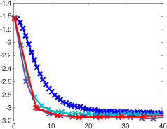
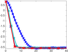
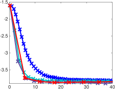
time (seconds)	time (seconds)	time (seconds)
(a) $\mathbb{E}(x)$	(b) $\mathbb{E}(x^{2})$	(c) $\mathbb{E}(\cos(wx+b))$

Figure 7: Results when using different numbers of gradient decent steps for solving (14). The setting is the same as that in Figure 2, but we conduct experiments using 1, 5, 10, 20 gradient steps when solving (14), and show their corresponding training time in the $x$-axis, and their mean square error for estimating $\mathbb{E}_{p}h$ (for the “testing” distributions) in the $y$-axis. The Langevin samplers we used have $T=10$ layers (Langevin update steps). The results are evaluated by drawing 1,000 samples from the trained samplers at different iterations of SVGD. The dimension of the Gaussian Mixtures is $d=50$.

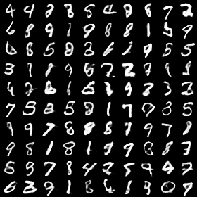
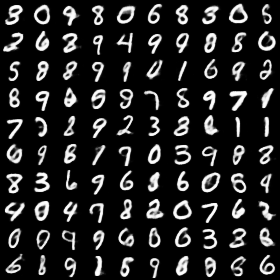
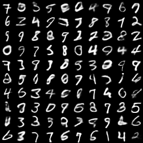
VAE-CNN	EVAE-CNN	ESteinVAE-CNN

Figure 8: Images generated by VAE-CNN, EVAE-CNN, and ESteinVAE-CNN

Appendix B Solving the Projection Step Using Different Numbers Gradient Steps

Amortized SVGD requires us to solve the projection step using either (13) or (14) at each iteration. In practice, we approximately solve it using only one step of gradient descent starting from the old values of $\eta$ for the sake of computational efficiency.

In order to study the trade-off of accuracy and computational cost here, we plot in Figure 7 the results when we solve Eq (14) using different numbers of gradient descent steps (the result is almost identical when we solve Eq (13) instead). We can see that when using more gradient steps, although the training time per iteration increases, the overall convergence speed may still improve, because it may take less iterations to converge. Figure 7 seems to suggest that using 5, 10, 20 steps gives better convergence than using a single step, but this may vary in different cases. We suggest to search for the best gradient step if the convergence speed is a primary concern. On the other hand, the number of gradient steps seems to have minor influence on the final result at the convergence as shown in Figure 7.

Appendix C Images Generated by Different VAEs

Figure 8 shows the images generated by the standard VAE-CNN, the entropy regularized VAE-CNN and ESteinVAE-CNN. We can see that both EVAE-CNN and ESteinVAE-CNN can generate images of good quality.

References

- Agakov & Barber (2004) Agakov, Felix V and Barber, David. An auxiliary variational method. In International Conference on Neural Information Processing, pp. 561–566. Springer, 2004.
- Andrieu & Thoms (2008) Andrieu, Christophe and Thoms, Johannes. A tutorial on adaptive mcmc. Statistics and Computing, 18(4):343–373, 2008.
- Balan et al. (2015) Balan, Anoop Korattikara, Rathod, Vivek, Murphy, Kevin P, and Welling, Max. Bayesian dark knowledge. In Advances in Neural Information Processing Systems, pp. 3438–3446, 2015.
- Briol et al. (2015) Briol, François-Xavier, Oates, Chris, Girolami, Mark, Osborne, Michael A, Sejdinovic, Dino, et al. Probabilistic integration: A role for statisticians in numerical analysis? arXiv preprint http://arxiv.org/abs/1512.00933, 2015.
- Burda et al. (2015) Burda, Yuri, Grosse, Roger, and Salakhutdinov, Ruslan. Importance weighted autoencoders. arXiv preprint arXiv:1509.00519, 2015.
- Chwialkowski et al. (2016) Chwialkowski, Kacper, Strathmann, Heiko, and Gretton, Arthur. A kernel test of goodness of fit. In Proceedings of the International Conference on Machine Learning (ICML), 2016.
- Delyon & Portier (2014) Delyon, Bernard and Portier, François. Integral approximation by kernel smoothing. arXiv preprint arXiv:1409.0733, 2014.
- Gershman & Goodman (2014) Gershman, Samuel J and Goodman, Noah D. Amortized inference in probabilistic reasoning. In Proceedings of the 36th Annual Conference of the Cognitive Science Society, 2014.
- Goodfellow et al. (2014) Goodfellow, Ian, Pouget-Abadie, Jean, Mirza, Mehdi, Xu, Bing, Warde-Farley, David, Ozair, Sherjil, Courville, Aaron, and Bengio, Yoshua. Generative adversarial nets. In Advances in Neural Information Processing Systems, pp. 2672–2680, 2014.
- Henmi et al. (2007) Henmi, Masayuki, Yoshida, Ryo, and Eguchi, Shinto. Importance sampling via the estimated sampler. Biometrika, 94(4):985–991, 2007.
- Hoffman et al. (2013) Hoffman, Matthew D, Blei, David M, Wang, Chong, and Paisley, John. Stochastic variational inference. JMLR, 2013.
- Kingma & Welling (2013) Kingma, Diederik P and Welling, Max. Auto-encoding variational Bayes. In Proceedings of the International Conference on Learning Representations (ICLR), 2013.
- Kingma et al. (2016) Kingma, Diederik P, Salimans, Tim, and Welling, Max. Improving variational inference with inverse autoregressive flow. arXiv preprint arXiv:1606.04934, 2016.
- Li et al. (2017) Li, Yingzhen, Turner, Richard E, and Liu, Qiang. Approximate inference with amortised mcmc. arXiv preprint arXiv:1702.08343, 2017.
- Liu & Lee (2016) Liu, Qiang and Lee, Jason D. Black-box importance sampling. https://arxiv.org/abs/1610.05247, 2016.
- Liu & Wang (2016) Liu, Qiang and Wang, Dilin. Stein variational gradient descent: A general purpose bayesian inference algorithm. arXiv preprint arXiv:1608.04471, 2016.
- Liu et al. (2016) Liu, Qiang, Lee, Jason D, and Jordan, Michael I. A kernelized Stein discrepancy for goodness-of-fit tests. In Proceedings of the International Conference on Machine Learning (ICML), 2016.
- Maclaurin et al. (2015) Maclaurin, Dougal, Duvenaud, David, and Adams, Ryan P. Early stopping is nonparametric variational inference. arXiv preprint arXiv:1504.01344, 2015.
- Mandt et al. (2016) Mandt, Stephan, Hoffman, Matthew D, and Blei, David M. A variational analysis of stochastic gradient algorithms. arXiv preprint arXiv:1602.02666, 2016.
- Mescheder et al. (2017) Mescheder, Lars, Nowozin, Sebastian, and Geiger, Andreas. Adversarial variational bayes: Unifying variational autoencoders and generative adversarial networks. arXiv preprint arXiv:1701.04722, 2017.
- Mohamed & Lakshminarayanan (2016) Mohamed, Shakir and Lakshminarayanan, Balaji. Learning in implicit generative models. arXiv preprint arXiv:1610.03483, 2016.
- Oates et al. (2017) Oates, Chris J, Girolami, Mark, and Chopin, Nicolas. Control functionals for Monte Carlo integration. Journal of the Royal Statistical Society, Series B, 2017.
- O’Hagan (1987) O’Hagan, Anthony. Monte Carlo is fundamentally unsound. Journal of the Royal Statistical Society. Series D (The Statistician), 36(2/3):247–249, 1987.
- O’Hagan (1991) O’Hagan, Anthony. Bayes–hermite quadrature. Journal of statistical planning and inference, 29(3):245–260, 1991.
- Paige & Wood (2016) Paige, Brooks and Wood, Frank. Inference networks for sequential monte carlo in graphical models. arXiv preprint arXiv:1602.06701, 2016.
- Pu et al. (2017) Pu, Yunchen, Gan, Zhe, Henao, Ricardo, Li, Chunyuan, Han, Shaobo, and Carin, Lawrence. Vae learning via stein variational gradient descent. In Advances in Neural Information Processing Systems (NIPS), 2017.
- Ranganath et al. (2016) Ranganath, R., Altosaar, J., Tran, D., and Blei, D.M. Operator variational inference. 2016.
- Rezende & Mohamed (2015) Rezende, Danilo Jimenez and Mohamed, Shakir. Variational inference with normalizing flows. In Proceedings of the International Conference on Machine Learning (ICML), 2015.
- Roberts & Rosenthal (2009) Roberts, Gareth O and Rosenthal, Jeffrey S. Examples of adaptive mcmc. Journal of Computational and Graphical Statistics, 18(2):349–367, 2009.
- Salimans et al. (2015) Salimans, Tim et al. Markov chain monte carlo and variational inference: Bridging the gap. In International Conference on Machine Learning, 2015.
- Welling & Teh (2011) Welling, Max and Teh, Yee W. Bayesian learning via stochastic gradient Langevin dynamics. In Proceedings of the International Conference on Machine Learning (ICML), 2011.
- Wu et al. (2016) Wu, Yuhuai, Burda, Yuri, Salakhutdinov, Ruslan, and Grosse, Roger. On the quantitative analysis of decoder-based generative models. arXiv preprint arXiv:1611.04273, 2016.