Nonlinear transverse cascade and sustenance of MRI-turbulence in Keplerian disks with an azimuthal magnetic field

Abstract

We investigate magnetohydrodynamic turbulence driven by the magnetorotational instability (MRI) in Keplerian disks with a nonzero net azimuthal magnetic field using shearing box simulations. As distinct from most previous studies, we analyze turbulence dynamics in Fourier (${\bf k}$-) space to understand its sustenance. The linear growth of MRI with azimuthal field has a transient character and is anisotropic in Fourier space, leading to anisotropy of nonlinear processes in Fourier space. As a result, the main nonlinear process appears to be a new type of angular redistribution of modes in Fourier space – the nonlinear transverse cascade – rather than usual direct/inverse cascade. We demonstrate that the turbulence is sustained by interplay of the linear transient growth of MRI (which is the only energy supply for the turbulence) and the transverse cascade. These two processes operate at large length scales, comparable to box size and the corresponding small wavenumber area, called vital area in Fourier space is crucial for the sustenance, while outside the vital area direct cascade dominates. The interplay of the linear and nonlinear processes in Fourier space is generally too intertwined for a vivid schematization. Nevertheless, we reveal the basic subcycle of the sustenance that clearly shows synergy of these processes in the self-organization of the magnetized flow system. This synergy is quite robust and persists for the considered different aspect ratios of the simulation boxes. The spectral characteristics of the dynamical processes in these boxes are qualitatively similar, indicating the universality of the sustenance mechanism of the MRI-turbulence.

1 Introduction

The problem of the onset and sustenance of turbulence in accretion disks lies at the basis of understanding different aspects of disk dynamics and evolution: secular redistribution of angular momentum yielding observationally obtained accretion rates, dynamo action and generation of magnetic fields and outflows, possibility of appearance of coherent structures (e.g., vortices, zonal flows, pressure bumps) that can form sites for planet formation. Investigations in this direction acquired new impetus and became more active since Balbus & Hawley (1991) demonstrated the relevance and significance of the magnetorotational instability (MRI) for disks. Today the MRI is considered as the most likely cause of magnetohydrodynamic (MHD) turbulence in disks and hence a driver agent of the above phenomena. Starting from the 1990s a vast number of analytical and numerical studies have investigated different aspects of linear and nonlinear evolution of the MRI in three-dimensional (3D) Keplerian disks using both local shearing box and global approaches for different configurations (unstratified and stratified, incompressible and compressible, with vertical and/or azimuthal magnetic fields having zero and nonzero net fluxes) at different domain sizes and resolutions (see e.g., Armitage, 2011; Fromang, 2013, for a review).

In this paper, we consider a local model of a disk threaded by a nonzero net azimuthal/toroidal magnetic field. The linear stability analysis showed that only non-axisymmetric perturbations can exhibit the MRI for this orientation of the background field (Balbus & Hawley, 1992; Ogilvie & Pringle, 1996; Terquem & Papaloizou, 1996; Papaloizou & Terquem, 1997; Brandenburg & Dintrans, 2006; Salhi et al., 2012; Shtemler et al., 2012). Such perturbations are, however, sheared by the disk’s differential rotation (shear) and as a result the MRI acquires a transient nature, while the flow stays exponentially, or spectrally stable. Nevertheless, as early seminal numerical simulations by Hawley et al. (1995) revealed, the transient MRI in the presence of an azimuthal field in fact causes transition to MHD turbulence. However, the transient growth itself, which in this case is the only available source of energy for turbulence, cannot ensure a long-term sustenance of the latter without appropriate nonlinear feedback. In other words, the role of nonlinearity becomes crucial: it lies at the heart of the sustenance of turbulence. Thus, the transition to turbulence in the presence of azimuthal field fundamentally differs from that in the case of the vertical field, where the MRI grows exponentially forming a channel flow, which, in turn, breaks down into turbulence due to secondary (parasitic) instabilities (Goodman & Xu, 1994; Hawley et al., 1995; Bodo et al., 2008; Pessah & Goodman, 2009; Latter et al., 2009; Pessah, 2010; Longaretti & Lesur, 2010; Murphy & Pessah, 2015).

The first developments of the MRI in magnetized disks in the 1990s coincided with the period of the breakthrough of the fluid dynamical community in understanding the dynamics of spectrally stable (i.e., without exponentially growing eigenmodes) hydrodynamic (HD) shear flows (see e.g., Reddy et al., 1993; Trefethen et al., 1993; Farrell & Ioannou, 1996; Schmid & Henningson, 2001; Schmid, 2007). The nonnormality of these flows, i.e., the nonorthogonality of the eigenfunctions of classical modal approach, had been demonstrated and its consequences – the transient/nonmodal growth of perturbations and the transition to turbulence were thoroughly analyzed. There are no exponentially growing modes in such flows and the turbulence is energetically supported only by the linear nonmodal growth of perturbations due to the shear flow nonnormality. Afterwards, the bypass concept of the onset and sustenance of turbulence in spectrally stable shear flows was formulated (see e.g., Gebhardt & Grossmann, 1994; Baggett et al., 1995; Grossmann, 2000). According to this concept, the turbulence is triggered and maintained by a subtle interplay of shear-induced linear transient growth and nonlinear processes. These processes appear to be strongly anisotropic in Fourier (${\bf k}$-) space due to the shear (Horton et al., 2010; Mamatsashvili et al., 2016) in contrast to classical isotropic and homogeneous forced turbulence without background shear.

Differentially rotating disks represent special case of shear flows and hence the effects of nonnormality inevitably play a key role in their dynamics (e.g., Chagelishvili et al., 2003; Mukhopadhyay et al., 2005; Zhuravlev & Razdoburdin, 2014; Razdoburdin & Zhuravlev, 2017). In particular, in magnetized disks, the nonmodal/transient growth of the MRI over intermediate (dynamical) times can be actually more relevant in many situations than its modal growth (Mamatsashvili et al., 2013; Squire & Bhattacharjee, 2014). Since in the present case of azimuthal field, the MRI exhibits only transient rather than exponential growth, the resulting turbulence, like in spectrally stable HD shear flows, is expected to be governed by a subtle cooperation of this nonmodal growth and nonlinear processes. As we showed previously (Mamatsashvili et al., 2014), this is indeed the case for an analogous two-dimensional (2D) MHD flow with linear shear and magnetic field parallel to it and the flow configuration considered here in fact represents its 3D generalization. So, our main goal is to investigate the spectral properties and sustaining dynamics of MHD turbulence driven by the transient amplification of the MRI in disks with a net nonzero azimuthal field.

The dynamics and statistics of MRI-driven MHD turbulence in Keplerian disk flows have been commonly analyzed and interpreted in physical space rather than in Fourier space. This also concerns studies of disks with nonzero net azimuthal magnetic field. Below we cite the most relevant ones. Hawley et al. (1995); Guan et al. (2009); Guan & Gammie (2011); Nauman & Blackman (2014); Ross et al. (2016) in the shearing box, and Fromang & Nelson (2006); Beckwith et al. (2011); Flock et al. (2011, 2012a); Sorathia et al. (2012); Hawley et al. (2013); Parkin & Bicknell (2013) in global disk simulations extensively investigated the dependence of the dynamics and saturation of the MRI-turbulence without explicit dissipation on the domain size, resolution and imposed azimuthal field strength. Fleming et al. (2000) in local model and Flock et al. (2012b) in global model addressed the influence of resistivity and established a critical value of magnetic Reynolds number for the existence of turbulence. Simon & Hawley (2009) and Meheut et al. (2015) included also viscosity together with resistivity and showed that at fixed field strength the saturation amplitude mainly depends on the magnetic Prandtl number, that is, the ratio of viscosity to resistivity, if the latter is larger than unity and the Reynolds number is high enough. On the other hand, at Prandtl numbers smaller than unity the turbulence sustenance is more delicate: it appears to be independent of the Prandtl number and mainly determined by the magnetic Reynolds number. Simon & Hawley (2009) attributed this behavior to the small-scale resistive dissipation processes (reconnection), which are thought to be central in the saturation process.

Part of these papers based on the local approximation (Hawley et al., 1995; Fleming et al., 2000; Nauman & Blackman, 2014; Meheut et al., 2015) do present analysis of energy density power spectrum, but in somewhat restricted manner by considering either averaging over wavevector angle, i.e., averages over spherical shells of constant $|{\bf k}|$, or slices along different directions in Fourier space. However, there are several studies of MRI turbulence also in the local approximation, but with nonzero net vertical magnetic flux (Lesur & Longaretti, 2011) and with zero net flux (Fromang & Papaloizou, 2007; Fromang et al., 2007; Simon et al., 2009; Davis et al., 2010), which go beyond energy spectrum and describe the dynamics of MRI- turbulence and associated energy injection (stresses) and nonlinear transfer processes in Fourier space, but again in a restricted manner by using shell-averaging procedure and/or reduced one-dimensional (1D) spectrum along a certain direction in Fourier space by integrating in the other two. However, as demonstrated by Hawley et al. (1995); Lesur & Longaretti (2011); Murphy & Pessah (2015) for MRI-turbulence (with net vertical field) and by our previous study of 2D MHD shear flow turbulence in Fourier space (Mamatsashvili et al., 2014), the power spectra and underlying dynamics are notably anisotropic due to shear, i.e., depend quite strongly also on the orientation of wavevector ${\bf k}$ in Fourier space rather than only on its magnitude $|{\bf k}|$. This is in contrast to a classical isotropic forced turbulence without background velocity shear, where energy cascade proceeds along ${\bf k}$ only (Biskamp, 2003). This shear-induced anisotropy also differs from the typical anisotropy of classical shearless MHD turbulence in the presence of a (strong) background magnetic field (Goldreich & Sridhar, 1995). It leads to anisotropy of nonlinear processes and particularly to the nonlinear transverse cascade (see below) that play a central role in the sustenance of turbulence in the presence of transient growth. Consequently, the shell-averaging done in the above studies is misleading, because it completely leaves out shear-induced spectral anisotropy, which is thus an essential ingredient of the dynamics of shear MHD turbulence. The recent works by Meheut et al. (2015) and Murphy & Pessah (2015) share a similar point of view, emphasizing the importance of describing anisotropic shear MRI-turbulence using a full 3D spectral analysis instead of using spherical shell averaging in Fourier space, which is applicable only for isotropic turbulence without shear. Such a generalized treatment is a main goal of this paper. In particular, Murphy & Pessah (2015) employ a new approach that consists in using invariant maps for characterizing anisotropy of MRI-driven turbulence in physical space and dissecting the 3D Fourier spectrum along the most relevant planes, as defined by the type of anisotropy of the flows.

As for the global disk studies cited above, relatively little attention is devoted to the dynamics of MRI-turbulence in Fourier space. This is, however, understandable, since in contrast to the cartesian shearing box model, global disk geometry makes it harder to perform Fourier analysis in all three, radial, azimuthal and meridional directions, so that these studies only consider azimuthal spectra integrated in other two directions.

Recently, we have numerically studied a cooperative interplay of linear transient growth and nonlinear processes ensuring the sustenance of nonlinear perturbations in HD and 2D MHD plane spectrally stable constant shear flows (Horton et al., 2010; Mamatsashvili et al., 2014, 2016). Performing the analysis of dynamical processes in Fourier space, we showed that the shear-induced spectral anisotropy gives rise to a new type of nonlinear cascade process that leads to transverse redistribution of modes in k-space, i.e. to a redistribution over wavevector angles. This process, referred to as the nonlinear transverse cascade, originates ultimately from flow shear and fundamentally differs from the canonical (direct and inverse) cascade processes accepted in classical Kolmogorov or Iroshnikov-Kraichnan (IK) theories of turbulence (see e.g., Biskamp, 2003). The new approach developed in these studies and the main results can be summarized as follows:
– identifying modes that play a key role in the sustaining process of the turbulence;
– defining a wavenumber area in Fourier space that is vital in the sustenance of turbulence;
– defining a range of aspect ratios of the simulation domain for which the dynamically important modes are fully taken into account;
– revealing the dominance of the nonlinear transverse cascade in the dynamics;
– showing that the turbulence is sustained by a subtle interplay between the linear transient (nonmodal) growth and the nonlinear transverse cascade.

In this paper, with the same spirit and goals in mind, we take the approach of Mamatsashvili et al. (2014) to investigate the dynamics and sustenance of MHD turbulence driven by the transient growth of MRI with a net nonzero azimuthal field in a Keplerian disk flow. We adopt the shearing box model of the disk (see e.g., Hawley et al., 1995), where the flow is characterized by constant shear rate, as that considered in that paper, except it is 3D, including rotation (Coriolis force) and vertical thermal stratification. To capture the spectral anisotropy of the MRI-turbulence, we analyze the linear and nonlinear dynamical processes and their interplay in 3D Fourier space in full without using the above-mentioned procedure of averaging over spherical shells of constant $k=|{\bf k}|$. So, our study is intended to be more general than the above-mentioned studies that also addressed the spectral dynamics of MRI-turbulence. One of our goals is to demonstrate the realization and efficiency of the transverse cascade and its role in the turbulence dynamics also in the 3D case, as we did for 2D MHD shear flow. Although in 3D perturbation modes are more diverse and, of course, modify the dynamics, still the essence of the cooperative interplay of linear (transient) and nonlinear (transverse cascade) processes should be preserved.

We pay particular attention to the choice of the aspect ratio of the simulation box, so as to encompass as full as possible the modes exhibiting the most effective amplification due to the transient MRI. To this aim, we apply the method of optimal perturbations, widely used in fluid dynamics for characterizing the nonmodal growth in spectrally stable shear flows (see e.g., Farrell & Ioannou, 1996; Schmid & Henningson, 2001; Zhuravlev & Razdoburdin, 2014), to the present MRI problem (see also Squire & Bhattacharjee, 2014). These are perturbations that undergo maximal transient growth during the dynamical time. In this framework, we define areas in Fourier space, where the transient growth is more effective – these areas cover small wavenumber modes. On the other hand, the simulation box includes only a discrete number of modes and minimum wavenumbers are set by its size. A dense population of modes in these areas of the effective growth in ${\bf k}$-space is then achieved by suitably choosing the box sizes. In particular, we show that simulations with elongated in the azimuthal direction boxes (i.e., with azimuthal size larger than radial one), do not fully account for this nonmodal effects, since the discrete wavenumbers of modes contained in such boxes scarcely cover the areas of efficient transient growth.

The paper is organized as follows. The physical model and derivation of dynamical equations in Fourier space is given in Section 2. Selection of the suitable aspect ratio of the simulation box based on the optimal growth calculations is made in Section 3. Numerical simulations of the MRI-turbulence at different aspect ratios of the simulation box are done in Section 4. In this Section we present also energy spectra, we determine dynamically active modes and delineate the vital area of turbulence, where the active modes and hence the sustaining dynamics are concentrated. The analysis of the interplay of the linear and nonlinear processes in Fourier space and the sustaining mechanism of the turbulence is described in Section 5. In this Section we also reveal the basic subcycle of the sustenance, describe the importance of the magnetic nonlinear term in the generation and maintenance of the zonal flow, examine the effect of the box aspect ratio and demonstrate the universality of the sustaining scheme. A summary and discussion are given in Section 6.

2 Physical model and equations

We consider the motion of an incompressible conducting fluid with constant kinematic viscosity $\nu$, thermal diffusivity $\chi$ and Ohmic resistivity $\eta$, in the shearing box centered at a radius $r_{0}$ and rotating with the disk at angular velocity $\Omega(r_{0})$. Adopting the Boussinesq approximation for vertical thermal stratification (Balbus & Hawley, 1991; Lesur & Ogilvie, 2010), the governing equations of the non-ideal MHD become

$$\frac{\partial{\bf U}}{\partial t}+({\bf U}\cdot\nabla){\bf U}=-\frac{1}{\rho}\nabla P+\frac{\left({\bf B}\cdot\nabla\right){\bf B}}{4\pi\rho}-2{\bf\Omega}\times{\bf U}\\ +2q{\Omega}^{2}x{\bf e}_{x}-\Lambda N^{2}\theta{\bf~{}e}_{z}+\nu\nabla^{2}{\bf U},$$ (1)

$$\frac{\partial\theta}{\partial t}+{\bf U}\cdot\nabla\theta=\frac{u_{z}}{\Lambda}+\chi\nabla^{2}\theta,$$ (2)

$$\frac{\partial{\bf B}}{\partial t}=\nabla\times\left({\bf U}\times{\bf B}\right)+\eta\nabla^{2}{\bf B},$$ (3)

$$\nabla\cdot{\bf U}=0,$$ (4)

$$\nabla\cdot{\bf B}=0,$$ (5)

where ${\bf e}_{x},~{}{\bf e}_{y},~{}{\bf e}_{z}$ are the unit vectors, respectively, along the radial $(x)$, azimuthal $(y)$ and vertical $(z)$ directions, $\rho$ is the density, ${\bf U}$ is the velocity, ${\bf B}$ is the magnetic field, $P$ is the total pressure, equal to the sum of the thermal and magnetic pressures, $\theta\equiv{\delta\rho}/\rho$ is the perturbation of the density logarithm (or entropy, since pressure perturbations are neglected in the Boussinesq approximation). Finally, $N^{2}$ is the Brunt-V$\ddot{\rm a}$is$\ddot{\rm a}$l$\ddot{\rm a}$ frequency squared that controls the stratification. It is assumed to be positive and spatially constant, equal to $N^{2}=0.25\Omega^{2}$, formally corresponding to a stably stratified (i.e., convectively stable) local model along the vertical $z$-axis (Lesur & Ogilvie, 2010). For dimensional correspondence with the usual Boussinesq approximation, we define a stratification length $\Lambda\equiv g/N^{2}$, where $g$ is the vertical component of the gravity. Note, however, that $\Lambda$ cancels out from the equations if we normalize the density logarithm by $\Lambda\theta\rightarrow\theta$, which will be used henceforth. So, here we take into account the effects of thermal stratification in a simple way. Bodo et al. (2012, 2013) studied more sophisticated models of stratified MRI-turbulence in the shearing box, treating thermal physics self-consistently with dynamical equations. The shear parameter $q=-d\ln\Omega/d\ln r$ is set to $q=3/2$ for a Keplerian disk.

Equations (1)-(5) have a stationary equilibrium solution – an azimuthal flow along the $y$-direction with linear shear of velocity in the the radial $x$-direction, ${\bf U}_{0}=(0,-q\Omega x,0)$, with the total pressure $P_{0}$, density $\rho_{0}$ and threaded by an azimuthal uniform background magnetic field, ${\bf B}_{0}=(0,B_{0y},0),B_{0y}>0$. This simple, but important configuration, which corresponds to a local version of a Keplerian flow with toroidal field, allows us to grasp the key effects of the shear on the perturbation dynamics and ultimately on a resulting turbulent state.

Consider perturbations of the velocity, total pressure and magnetic field about the equilibrium, ${\bf u}={\bf U}-{\bf U}_{0},p=P-P_{0},{\bf b}={\bf B}-{\bf B}_{0}$. Substituting them into Equations (1)-(5) and rearranging the nonlinear terms with the help of divergence-free conditions (4) and (5), we arrive to the system (A1)-(A9) governing the dynamics of perturbations with arbitrary amplitude that is given in Appendix. These equations are solved within a box with sizes $(L_{x},L_{y},L_{z})$ and resolutions $(N_{x},N_{y},N_{z})$, respectively, in the $x,y,z-$directions. We use standard for the shearing box boundary conditions: shearing-periodic in $x$ and periodic in $y$ and $z$ (Hawley et al., 1995). For stratified disks, outflow boundary conditions in the vertical direction are more appropriate, however, in the present study, as mentioned above, we adopt a local approximation in $z$ with spatially constant $N^{2}$ that justifies our choice of the periodic boundary conditions in this direction (Lesur & Ogilvie, 2010). This does not affect the main dynamical processes in question.

2.1 Energy equation

The perturbation kinetic, thermal and magnetic energy densities are defined, respectively, as

$$E_{K}=\frac{1}{2}\rho_{0}{\bf u}^{2},~{}~{}~{}E_{th}=\frac{1}{2}\rho_{0}N^{2}\theta^{2},~{}~{}~{}E_{M}=\frac{{\bf b}^{2}}{8\pi}.$$

From the main Equations (A1)-(A9) and the shearing box boundary conditions, after some algebra, we can readily derive the evolution equations for the volume-averaged kinetic, thermal and magnetic energy densities

$$\frac{d}{dt}\langle E_{K}\rangle=q\Omega\left\langle\rho_{0}u_{x}u_{y}\right\rangle-N^{2}\left\langle\rho_{0}\theta u_{z}\right\rangle+\frac{1}{4\pi}\left\langle{\bf B}_{0}{\bf u}\otimes\nabla{\bf b}\right\rangle\\ -\frac{1}{4\pi}\left\langle{\bf b}{\bf b}\otimes\nabla{\bf u}\right\rangle-\rho_{0}\nu\langle\left(\nabla{\bf u}\right)^{2}\rangle,$$ (6)

$$\frac{d}{dt}\langle E_{th}\rangle=N^{2}\left\langle\rho_{0}\theta u_{z}\right\rangle-\rho_{0}N^{2}\chi\langle\left(\nabla\theta\right)^{2}\rangle,$$ (7)

$$\frac{d}{dt}\langle E_{M}\rangle=q\Omega\left\langle-\frac{b_{x}b_{y}}{4\pi}\right\rangle+\frac{1}{4\pi}\left\langle{\bf B}_{0}{\bf b}\otimes\nabla{\bf u}\right\rangle\\ +\frac{1}{4\pi}\left\langle{\bf b}{\bf b}\otimes\nabla{\bf u}\right\rangle-\frac{\eta}{4\pi}\langle\left(\nabla{\bf b}\right)^{2}\rangle,$$ (8)

where the angle brackets denote an average over the box. Adding up Equations (6)-(8), the cross terms of linear origin on the right hand side (rhs), proportional to $N^{2}$ and ${\bf B}_{0}$ (which describe kinetic-thermal and kinetic-magnetic energy exchange, respectively) and the nonlinear terms cancel out because of the boundary conditions. As a result, we obtain the equation for the total energy density $E=E_{K}+E_{th}+E_{M}$,

$$\frac{d\langle E\rangle}{dt}=q\Omega\left\langle\rho_{0}u_{x}u_{y}-\frac{b_{x}b_{y}}{4\pi}\right\rangle\\ -\rho_{0}\nu\langle\left(\nabla{\bf u}\right)^{2}\rangle-\rho_{0}N^{2}\chi\langle\left(\nabla\theta\right)^{2}\rangle-\frac{\eta}{4\pi}\langle\left(\nabla{\bf b}\right)^{2}\rangle.$$ (9)

The first term on the rhs of Equation (9) is the flow shear, $q\Omega$, multiplied by the volume-averaged total stress. The total stress is a sum of the Reynolds, $\rho_{0}u_{x}u_{y}$, and Maxwell, $-b_{x}b_{y}/4\pi$, stresses that describe, respectively, exchange of kinetic and magnetic energies between perturbations and the background flow in Equations (6) and (8). Note that they originate from the linear terms proportional to shear in Equations (A2) and (A6). The stresses also determine the rate of angular momentum transport (e.g., Hawley et al., 1995; Balbus, 2003) and thus are one of the important diagnostics of turbulence. The negative definite second, third and fourth terms describe energy dissipation due to viscosity, thermal diffusivity and resistivity, respectively. Note that a net contribution from the nonlinear terms has canceled out in the total energy evolution Equation (9) after averaging over the box. Thus, only Reynolds and Maxwell stresses can supply perturbations with energy, extracting it from the background flow due to the shear. In the case of the MRI-turbulence studied below, these stresses ensure energy injection into turbulent fluctuations. The nonlinear terms, not directly tapping into the flow energy and therefore not changing the total perturbation energy, act only to redistribute energy among different wavenumbers as well as among components of velocity and magnetic field (see below). In the absence of shear ($q=0$), the contribution from the Reynolds and Maxwell stresses disappears in Equation (9) and hence the total perturbation energy cannot grow, gradually decaying due to dissipation.

2.2 Spectral representation of the equations

Before proceeding further, we normalize the variables by taking $\Omega^{-1}$ as the unit of time, the disk scale height $H$ as the unit of length, $\Omega H$ as the unit of velocity, $\Omega H\sqrt{4\pi\rho_{0}}$ as the unit of magnetic field and $\rho_{0}\Omega^{2}H^{2}$ as the unit of pressure and energy. Viscosity, thermal diffusivity and resistivity are measured, respectively, by Reynolds number, ${\rm Re}$, Péclet number, ${\rm Pe}$, and magnetic Reynolds number, ${\rm Rm}$, defined as

$${\rm Re}=\frac{\Omega H^{2}}{\nu},~{}~{}~{}{\rm Pe}=\frac{\Omega H^{2}}{\chi},~{}~{}~{}{\rm Rm}=\frac{\Omega H^{2}}{\eta}.$$

All the simulations share the same ${\rm Re}={\rm Pe}={\rm Rm}=3200$ (i.e., the magnetic Prandtl number ${\rm Pm}={\rm Rm}/{\rm Re}=1$). The strength of the imposed background uniform azimuthal magnetic field is measured by a parameter $\beta=2\Omega^{2}H^{2}/v_{A}^{2}$, which we fix to $\beta=200$, where $v_{A}=B_{0y}/(4\pi\rho_{0})^{1/2}$ is the corresponding Alfvén speed. In the incompressible case, this parameter is a proxy of the usual plasma $\beta$ parameter (Longaretti & Lesur, 2010), since the sound speed in thin disks is $c_{s}\sim\Omega H$. In this non-dimensional units, the mean field becomes $B_{0y}=\sqrt{2/\beta}=0.1.$

Our primary interest lies in the spectral aspect of the dynamics, so we start with decomposing the perturbations $f\equiv({\bf u},p,\theta,{\bf b})$ into spatial Fourier harmonics/modes

$$f({\bf r},t)=\int\bar{f}({\bf k},t)\exp\left({\rm i}{\bf k}\cdot{\bf r}\right)d^{3}{\bf k}$$ (10)

where $\bar{f}\equiv(\bar{\bf u},\bar{p},\bar{\theta},\bar{\bf b})$ denotes the corresponding Fourier transforms. Substituting decomposition (10) into perturbation Equations (A1)-(A9), taking into account the above normalization and eliminating the pressure (see derivation in Appendix), we obtain the following evolution equations for the quadratic forms of the spectral velocity, logarithmic density (entropy) and magnetic field:

$$\frac{\partial}{\partial t}\frac{|\bar{u}_{x}|^{2}}{2}=-qk_{y}\frac{\partial}{\partial k_{x}}\frac{|\bar{u}_{x}|^{2}}{2}+{\cal H}_{x}+{\cal I}_{x}^{(u\theta)}+{\cal I}_{x}^{(ub)}+{\cal D}_{x}^{(u)}+{\cal N}_{x}^{(u)},$$ (11)

$$\frac{\partial}{\partial t}\frac{|\bar{u}_{y}|^{2}}{2}=-qk_{y}\frac{\partial}{\partial k_{x}}\frac{|\bar{u}_{y}|^{2}}{2}+{\cal H}_{y}+{\cal I}_{y}^{(u\theta)}+{\cal I}_{y}^{(ub)}+{\cal D}_{y}^{(u)}+{\cal N}_{y}^{(u)},$$ (12)

$$\frac{\partial}{\partial t}\frac{|\bar{u}_{z}|^{2}}{2}=-qk_{y}\frac{\partial}{\partial k_{x}}\frac{|\bar{u}_{z}|^{2}}{2}+{\cal H}_{z}+{\cal I}_{z}^{(u\theta)}+{\cal I}_{z}^{(ub)}+{\cal D}_{z}^{(u)}+{\cal N}_{z}^{(u)},$$ (13)

$$\frac{\partial}{\partial t}\frac{|\bar{\theta}|^{2}}{2}=-qk_{y}\frac{\partial}{\partial k_{x}}\frac{|\bar{\theta}|^{2}}{2}+{\cal I}^{(\theta u)}+{\cal D}^{(\theta)}+{\cal N}^{(\theta)},$$ (14)

$$\frac{\partial}{\partial t}\frac{|\bar{b}_{x}|^{2}}{2}=-qk_{y}\frac{\partial}{\partial k_{x}}\frac{|\bar{b}_{x}|^{2}}{2}+{\cal I}_{x}^{(bu)}+{\cal D}_{x}^{(b)}+{\cal N}_{x}^{(b)},$$ (15)

$$\frac{\partial}{\partial t}\frac{|\bar{b}_{y}|^{2}}{2}=-qk_{y}\frac{\partial}{\partial k_{x}}\frac{|\bar{b}_{y}|^{2}}{2}+{\cal M}+{\cal I}_{y}^{(bu)}+{\cal D}_{y}^{(b)}+{\cal N}_{y}^{(b)},$$ (16)

$$\frac{\partial}{\partial t}\frac{|\bar{b}_{z}|^{2}}{2}=-qk_{y}\frac{\partial}{\partial k_{x}}\frac{|\bar{b}_{z}|^{2}}{2}+{\cal I}_{z}^{(bu)}+{\cal D}_{z}^{(b)}+{\cal N}_{z}^{(b)}.$$ (17)

These seven dynamical equations in Fourier space, which are the basis for the subsequent analysis, describe processes of linear, $~{}{\cal H}_{i}({\bf k},t)$, ${\cal I}_{i}^{(u\theta)}({\bf k},t)$, ${\cal I}^{(\theta u)}({\bf k},t)$, ${\cal I}_{i}^{(ub)}({\bf k},t)$, ${\cal I}_{i}^{(bu)}({\bf k},t)$, ${\cal M}({\bf k},t)$, and nonlinear, $~{}{\cal N}_{i}^{(u)}({\bf k},t)$, ${\cal N}^{(\theta)}({\bf k},t)$, ${\cal N}_{i}^{(b)}({\bf k},t)$, origin, where the index $i=x,y,z$ henceforth. ${\cal D}_{i}^{(u)}({\bf k},t)$, ${\cal D}^{(\theta)}({\bf k},t)$, ${\cal D}_{i}^{(b)}({\bf k},t)$ describe the effects of viscous, thermal and resistive dissipation as a function of wavenumber and are negative definite. These terms come from the respective linear and nonlinear terms in main Equations (A1)-(A7) and their explicit expressions are derived in Appendix. In the turbulent regime, these basic linear and nonlinear processes are subtly intertwined, so before embarking on calculating and analyzing these terms from the simulation data, we first describe them in more detail below. Equations (11)-(17) serve as a mathematical basis for our main goal – understanding the character of the interplay of the dynamical processes sustaining the MRI-turbulence. Since we consider a finite box in physical space, the perturbation dynamics also depends on the smallest wavenumber available in the box (see Section 3), which is set by its sizes $L_{x},L_{y},L_{z}$ and is a free parameter in the shearing box.

To get a general feeling, as in Simon et al. (2009); Lesur & Longaretti (2011), we derive also equations for the spectral kinetic energy, ${\cal E}_{K}=(|\bar{u}_{x}|^{2}+|\bar{u}_{y}|^{2}+|\bar{u}_{z}|^{2})/2$, by combining Equations (11)-(13),

$$\frac{\partial{\cal E}_{K}}{\partial t}=-qk_{y}\frac{\partial{\cal E}_{K}}{\partial k_{x}}+{\cal H}+{\cal I}^{(u\theta)}+{\cal I}^{(ub)}+{\cal D}^{(u)}+{\cal N}^{(u)},$$ (18)

where

$${\cal H}=\sum_{i}{\cal H}_{i}=\frac{q}{2}(\bar{u}_{x}\bar{u}_{y}^{\ast}+\bar{u}_{x}^{\ast}\bar{u}_{y}),$$

$${\cal I}^{(u\theta)}=\sum_{i}{\cal I}_{i}^{(u\theta)},~{}~{}~{}~{}{\cal I}^{(ub)}=\sum_{i}{\cal I}_{i}^{(ub)},$$

$${\cal D}^{(u)}=\sum_{i}{\cal D}_{i}^{(u)}=-\frac{2k^{2}}{\rm Re}{\cal E}_{K},~{}~{}~{}{\cal N}^{(u)}=\sum_{i}{\cal N}^{(u)}_{i}$$

and for the spectral magnetic energy, ${\cal E}_{M}=(|\bar{b}_{x}|^{2}+|\bar{b}_{y}|^{2}+|\bar{b}_{z}|^{2})/2$, by combining Equations (15)-(17),

$$\frac{\partial{\cal E}_{M}}{\partial t}=-qk_{y}\frac{\partial{\cal E}_{M}}{\partial k_{x}}+{\cal M}+{\cal I}^{(bu)}+{\cal D}^{(b)}+{\cal N}^{(b)},$$ (19)

where

$${\cal M}=-\frac{q}{2}(\bar{b}_{x}\bar{b}_{y}^{\ast}+\bar{b}_{x}^{\ast}\bar{b}_{y}),~{}~{}~{}~{}{\cal I}^{(bu)}=\sum_{i}{\cal I}_{i}^{(bu)}=-{\cal I}^{(ub)},$$

$${\cal D}^{(u)}=\sum_{i}{\cal D}_{i}^{(u)}=-\frac{2k^{2}}{\rm Rm}{\cal E}_{M},~{}~{}~{}{\cal N}^{(b)}=\sum_{i}{\cal N}^{(b)}_{i}.$$

The equation of the thermal energy, ${\cal E}_{th}=N^{2}|\theta|^{2}/2$, is straightforward to derive by multiplying Equation (14) just by $N^{2}$, so we do not write it here. Besides, we will see below that the thermal energy is much less than the magnetic and kinetic energies, so the thermal processes have a minor contribution in forming the final picture of the turbulence. Similarly, we get the equation for the total spectral energy of perturbations, ${\cal E}={\cal E}_{K}+{\cal E}_{th}+{\cal E}_{M}$,

$$\frac{\partial{\cal E}}{\partial t}=-qk_{y}\frac{\partial{\cal E}}{\partial k_{x}}+{\cal H}+{\cal M}+{\cal D}^{(u)}+N^{2}{\cal D}^{(\theta)}\\ +{\cal D}^{(b)}+{\cal N}^{(u)}+N^{2}{\cal N}^{(\theta)}+{\cal N}^{(b)}.$$ (20)

One can distinguish six basic processes, five of linear and one of nonlinear origin, in Equations (11) and (17) (and therefore in energy Equations 18 and 19) that underlie the perturbation dynamics:

1. The first terms on the rhs of Equations (11)-(17), $-qk_{y}\partial(.)/\partial k_{x}$, describe the linear “drift” of the related quadratic forms parallel to the $k_{x}$-axis with the normalized velocity $qk_{y}$. These terms are of linear origin, arising from the convective derivative on the lhs of the main Equations (A1)-(A7) and therefore correspond to the advection by the background flow. In other words, background shear makes the spectral quantities (Fourier transforms) drift in ${\bf k}-$space, non-axisymmetric harmonics with $k_{y}>0$ and $k_{y}<0$ travel, respectively, along and opposite the $k_{x}-$axis at a speed $|qk_{y}|$, whereas the ones with $k_{y}=0$ are not advected by the flow. This drift in Fourier space is equivalent to the time-varying radial wavenumber, $k_{x}(t)=k_{x}(0)+q\Omega k_{y}t$, in the linear analysis of non-axisymmetric shearing waves in magnetized disks (e.g., Balbus & Hawley, 1992; Johnson, 2007; Pessah & Chan, 2012). In the energy Equations (18) and (19), the spectral energy drift, of course, does not change the total kinetic and magnetic energies, since $\int d^{3}{\bf k}\partial(k_{y}{\cal E}_{K,M})/\partial k_{x}=0$.

2. The second rhs terms of Equations (11)-(13), ${\cal H}_{i}$, and Equation (16), ${\cal M}$, are also of linear origin associated with the shear (Equations B20-B22 and B34), i.e., originate from the linear terms proportional to the shear parameter in Equations (A2) and (A6). They describe the interaction between the flow and individual Fourier modes, where the velocity components $|\bar{u}_{i}|^{2}$ and the azimuthal field perturbation $|\bar{b}_{y}|^{2}$ can grow, respectively, due to ${\cal H}_{i}$ and ${\cal M}$, at the expense of the flow. In the present case, such amplification is due to the linear azimuthal MRI fed by the shear. In the presence of the mean azimuthal field, only non-axisymmetric modes exhibit the MRI and since they also undergo the drift in ${\bf k}-$space, their amplification acquires a transient nature (Balbus & Hawley, 1992; Papaloizou & Terquem, 1997; Brandenburg & Dintrans, 2006; Salhi et al., 2012; Shtemler et al., 2012). From the expressions (B20)-(B22) and (B34), we can see that ${\cal H}_{i}$ and ${\cal M}$ are related to the volume-averaged nondimensional Reynolds and Maxwell stresses entering energy Equations (6) and (8) through

   $$q\langle u_{x}u_{y}\rangle=\int{\cal H}d^{3}{\bf k},~{}~{}~{}~{}~{}q\langle-b_{x}b_{y}\rangle=\int{\cal M}d^{3}{\bf k},$$

   where ${\cal H}=\sum_{i}{\cal H}_{i}$, and hence represent, respectively, the spectra of the Reynolds and Maxwell stresses, acting as the source, or injection of kinetic and magnetic energies for perturbation modes at each wavenumber (see Equations 18 and 19) (see also Fromang & Papaloizou, 2007; Simon et al., 2009; Davis et al., 2010; Lesur & Longaretti, 2011).

3. the cross terms, ${\cal I}_{i}^{(u\theta)}$ and ${\cal I}^{(\theta u)}$ (Equations B23 and B28) describe, respectively, the effect of the thermal process on the $i$-component of the velocity, $\bar{u}_{i}$, and the effect of the $z$-component of the velocity on the logarithmic density (entropy) for each mode. These terms are also of linear origin, related to the Brunt-V$\ddot{\rm a}$is$\ddot{\rm a}$l$\ddot{\rm a}$ frequency squared $N^{2}$, and come from the corresponding linear terms in Equations (A3) and (A4). They are not a source of new energy, as $\sum_{i}{\cal I}_{i}^{(u\theta)}+N^{2}{\cal I}^{(\theta u)}=0$, but rather characterize exchange between kinetic and thermal energies (Equation 14 and 18), so they cancel out in the total spectral energy Equation (20).

4. the second type of cross terms, ${\cal I}_{i}^{(ub)}$ and ${\cal I}_{i}^{(bu)}$ (Equations B24 and B35), describe, respectively, the influence of the $i$-component of the magnetic field, $\bar{b}_{i}$, on the same component of the velocity, $\bar{u}_{i}$, and vice versa for each mode. These terms are of linear origin too, proportional to the mean field $B_{0y}$, and originate from the corresponding terms in Equations (A1)-(A3) and (A5)-(A7). From the definition it follows that ${\cal I}_{i}^{(ub)}=-{\cal I}_{i}^{(bu)}$ and hence these terms also do not generate new energy for perturbations, but rather exchange between kinetic and magnetic energies (Equations 18 and 19). They also cancel out in the total spectral energy equation.

5. The terms ${\cal D}_{i}^{(u)}$, ${\cal D}^{(\theta)}$ and ${\cal D}_{i}^{(b)}$ (Equations B25, B29 and B36) describe, respectively, dissipation of velocity, logarithmic density (entropy) and magnetic field for each wavenumber. They are obviously of linear origin and negative definite. Comparing these dissipation terms with the energy-supplying terms ${\cal H}_{i}$ and ${\cal M}$, we see that the dissipation is at work at large wavenumbers $k\gtrsim k_{D}\equiv{\rm min}(\sqrt{\rm Re},\sqrt{\rm Pe},\sqrt{\rm Rm})$.

6. The terms ${\cal N}_{i}^{(u)}$, $\cal N^{(\theta)}$ and ${\cal N}_{i}^{(b)}$ (Equations B26, B30 and B37) originate from the nonlinear terms in main Equations (A1)-(A7) and therefore describe redistributions, or transfers/cascades of the squared amplitudes, respectively, of the $i$-component of the velocity, $|\bar{u}_{i}|^{2}$, entropy, $|\bar{\theta}|^{2}$, and the $i$-component of the magnetic field, $|\bar{b}_{i}|^{2}$, over wavenumbers in $\textbf{k}-$space as well as among each other via nonlinear triad interactions. Similarly, the above-defined ${\cal N}^{(u)}$, $N^{2}{\cal N}^{(\theta)}$, ${\cal N}^{(b)}$ describe nonlinear transfers of kinetic, thermal and magnetic energies, respectively. It follows from the definition of these terms that their sum integrated over an entire Fourier space is zero,

   $$\int[{\cal N}^{(u)}({\bf k},t)+N^{2}{\cal N}^{(\theta)}({\bf k},t)+{\cal N}^{(b)}({\bf k},t)]d^{3}{\bf k}=0,$$ (21)

   which is, in fact, a direct consequence of cancelation of the nonlinear terms in the total energy Equation (9) in physical space. This implies that the main effect of nonlinearity is only to redistribute (scatter) energy (drawn from the background flow by Reynolds and Maxwell stresses) of the kinetic, thermal and magnetic components over wavenumbers and among each other, while leaving the total spectral energy summed over all wavenumbers unchanged. The nonlinear transfer functions (${\cal N}^{(u)}$, ${\cal N}^{(\theta)}$, ${\cal N}^{(b)}$) play a central role in MHD turbulence theory – they determine cascades of energies in k-space, leading to the development of their specific spectra (e.g., Verma, 2004; Alexakis et al., 2007; Teaca et al., 2009; Sundar et al., 2017). These transfer functions are one of the main focus of the present analysis. One of our main goals is to explore how they operate in the presence of the azimuthal field MRI in disks and ultimately of the shear. Specifically, below we will show that, like in 2D HD and MHD shear flows we studied before (Horton et al., 2010; Mamatsashvili et al., 2014), energy spectra, energy-injection as well as nonlinear transfers are also anisotropic in the quasi-steady MRI-turbulence, resulting in the redistribution of power among wavevector angles in $\textbf{k}-$space, i.e., the nonlinear transverse cascade.

Having described all the terms in spectral equations, we now turn to the total spectral energy Equation (20). Each mode drifting parallel to the $k_{x}-$axis, go through a dynamically important region in Fourier space, which we call the vital area, where energy-supplying linear terms, ${\cal H}$ and ${\cal M}$, and redistributing nonlinear terms, ${\cal N}^{(u)}$, ${\cal N}^{(\theta)}$, ${\cal N}^{(b)}$ operate. The net effect of the nonlinear terms in the total spectral energy budget over all wavenumbers is zero according to Equation (21). Thus, the only source for the total perturbation energy is the integral over an entire ${\bf k}$-space $\int({\cal H}+{\cal M})d^{3}{\bf k}$ that extracts energy from a vast reservoir of shear flow and injects it into perturbations. Since the terms ${\cal H}$ and ${\cal M}$, as noted above, are of linear origin, the energy extraction and perturbation growth mechanisms (the azimuthal MRI) are essentially linear by nature. The role of nonlinearity is to continually provide, or regenerate those modes in ${\bf k}$-space that are able to undergo the transient MRI, drawing on mean flow energy, and in this way feed the nonlinear state over long times. This scenario of a sustained state, based on a subtle cooperation between linear and nonlinear processes, is a keystone of the bypass concept of turbulence in spectrally stable HD shear flows (Gebhardt & Grossmann, 1994; Baggett et al., 1995; Grossmann, 2000; Chapman, 2002).

3 Optimization of the box aspect ratio – linear analysis

It is well known from numerical simulations of MRI-turbulence that its dynamics (saturation) generally depends on the aspect ratio ($L_{y}/L_{x}$, $L_{x}/L_{z}$) of a computational box (e.g., Hawley et al., 1995; Bodo et al., 2008; Guan et al., 2009; Johansen et al., 2009; Shi et al., 2016). In order to understand this dependence and hence appropriately select the aspect ratio in simulations, in our opinion, one should take into account as fully as possible the nonmodal growth of the MRI during intermediate (dynamical) timescales, because it can ultimately play an important role in the turbulence dynamics (Squire & Bhattacharjee, 2014). However, this is often overlooked in numerical studies. So, in this Section, we identify the aspect ratios of the preselected boxes that better take into account the linear transient growth process.

In fluid dynamics, the linear transient growth of perturbations in shear flows is usually quantified using the formalism of optimal perturbations (Farrell & Ioannou, 1996; Schmid & Henningson, 2001; Schmid, 2007). This approach has already been successfully applied to (magnetized) disk flows (Mukhopadhyay et al., 2005; Zhuravlev & Razdoburdin, 2014; Squire & Bhattacharjee, 2014; Razdoburdin & Zhuravlev, 2017). Such perturbations yield maximum linear nonmodal growth during finite times and therefore are responsible for most of the energy extraction from the background flow. So, in this framework, we quantify the linear nonmodal optimal amplification of the azimuthal MRI as a function of mode wavenumbers for the same parameters adopted in the simulations.

In the shearing box, the radial wavenumber of each non-axisymmetric perturbation mode (shearing wave) changes linearly with time due to shear, $k_{x}(t)=k_{x}(0)+q\Omega k_{y}t$. The maximum possible amplification of the total energy ${\cal E}={\cal E}_{K}+{\cal E}_{th}+{\cal E}_{M}$ of a shearing wave, with an initial wavenumber ${\bf k}(0)=(k_{x}(0),k_{y},k_{z})$ by a specific (dynamical) time $t_{d}$ is given by

$$G({\bf k}(t_{d}))=\max_{\bar{f}(0)}\frac{{\cal E}({\bf k}(t_{d}))}{{\cal E}({\bf k}(0))},$$ (22)

where the maximum is taken over all initial conditions $\bar{f}(0)$ with a given energy ${\cal E}({\bf k}(0))$. The final state at $t_{d}$ and the corresponding energy ${\cal E}({\bf k}(t_{d}))$ are found from the initial state at $t=0$ by integrating the linearized version of spectral Equations (B1)-(B9) in time for each shearing wave and finding a propagator matrix connecting the initial and final states. Then, expression (22) is usually calculated by means of the singular value decomposition of the propagator matrix. The square of the largest singular value then gives the optimal growth factor $G$ for this set of wavenumbers. The corresponding initial conditions, leading to this highest growth at $t_{d}$ are called optimal perturbations. (A reader interested in the details of these calculations is referred to Squire & Bhattacharjee (2014), where the formalism of optimal growth and optimal perturbations in MRI-active disks, which is adopted here, is described to a greater extent.) Reference time, during which to calculate the nonmodal growth, is generally arbitrary. We choose it equal to the characteristic ($e$-folding) time of the most unstable MRI mode, $t_{d}=1/\gamma_{max}=1.33\Omega^{-1}$, where $\gamma_{max}=0.75\Omega$ is its growth rate (Balbus, 2003; Ogilvie & Pringle, 1996), since it is effectively a dynamical time as well.

Figure 1 shows $G$ in $(k_{x},k_{y})-$plane at fixed $k_{z}$ as well as its value maximized over the initial $k_{x}(0)$, $G_{max}=\max_{k_{x}(0)}G$, represented as a function of $k_{y},k_{z}$. Because of the $k_{x}$-drift, the optimal mode with some initial radial wavenumber $k_{x}(0)$, at $t_{d}$ will have the wavenumber $k_{x}(t_{d})=k_{x}(0)+qk_{y}t_{d}$. In the top panel, $G$ is represented as a function of this final wavenumber $k_{x}(t_{d})$. Because of the shear, the typical distribution at fixed $k_{z}$ is inclined towards the $k_{x}$-axis, having larger values on the $k_{x}/k_{y}>0$ side (red region). The most effective nonmodal MRI amplification occurs at smaller wavenumbers, in the areas marked by dark red in both $(k_{x},k_{y})$ and $(k_{y},k_{z})$-planes in Figure 1. Thus, the growth of the MRI during the dynamical time appears to favor smaller $k_{z}$ (see also Squire & Bhattacharjee, 2014), as opposed to the transient growth of the azimuthal MRI often calculated over times much longer than the dynamical time, which is the more effective the larger is $k_{z}$ (Balbus & Hawley, 1992; Papaloizou & Terquem, 1997). Obviously, the growth over such long timescales is irrelevant for the nonlinear (turbulence) dynamics.

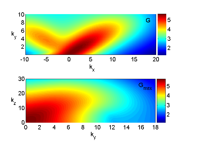
Figure 1: (upper panel) Optimal nonmodal growth factor, $G$, in $(k_{x},k_{y})$-plane at $t_{d}=1.33$ and $k_{z}/2\pi=1$ (which is the same as $k_{z}=1$ in new mode number notations used in the next Sections). (lower panel) Maximized over initial $k_{x}(0)$ growth factor, $G_{max}$, as a function of $k_{y}$ and $k_{z}$.

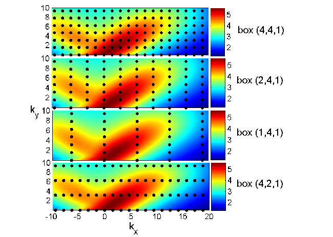
Figure 2: Discrete modes (black dots) contained in each simulation box superimposed on the distribution of $G$ in $(k_{x},k_{y})$-plane from the upper panel of Figure 1. From all the selected boxes, the box $(4,4,1)$ contains most of the effectively amplified modes.

In the simulation box, however, the wavenumber spectrum is inherently discrete, with smallest wavenumbers being defined by the box size $(L_{x},L_{y},L_{z})$ as $k_{i,min}=2\pi/L_{i}$, while other wavenumbers being multiples of them. We take $L_{z}=1$ (i.e., $L_{z}=H$ in dimensional units) and mainly consider four aspect ratios $(L_{x},L_{y},L_{z})=(4,4,1),~{}(2,4,1),~{}(1,4,1),~{}(4,2,1)$. Figure 2 shows the modes (black dots) in each box superimposed on the map of $G$ in $(k_{x},k_{y})$-plane from Figure 1 for the first vertical harmonics with $k_{z,min}$, or equivalently $k_{z}=1$ (in new notations used below). We see that from among these four boxes, the box $(4,4,1)$ contains the largest possible number of modes in the area of the effective transient growth and therefore best accounts for the role of the nonmodal effects in the energy exchange processes in the case of turbulence. Of course, further increasing $L_{x}$ and $L_{y}$ leads to larger number of modes in the area of effective growth, however, as also seen from Figure 2, already for the box $(4,4,1)$ this area appears to be sufficiently well populated with modes, i.e., enough resolution (measured in terms of $\Delta k_{i}=2\pi/L_{i}$) is achieved in Fourier space to adequately capture the nonmodal effects. To ascertain this, we also carried out a simulation for the box $(8,8,1)$ and found that the ratio of the number of the active modes (i.e., the number in the growth area) to the total number of modes in this larger box is almost the same as for the box $(4,4,1)$. Consequently, these boxes should give qualitatively similar dynamical pictures in Fourier space. For this reason, below we choose the box $(4,4,1)$ as fiducial and present only some results for other boxes for comparison at the end of Section 5.

4 Simulations and general characteristics

The main Equations (A1)-(A9) are solved using the pseudo-spectral code SNOOPY (Lesur & Longaretti, 2007). It is a general-purpose code, solving HD and MHD equations, including shear, rotation, stratification and several other physical effects in the shearing box model. Fourier transforms are computed using the FFTW library, taking also into account the drift of radial wavenumber $k_{x}(t)$ in ${\bf k}$-space due to shear in order to comply with the shearing-periodic boundary conditions. Nonlinear terms are computed using a pseudo-spectral algorithm (Canuto et al., 1988), and antialiasing is enforced using the $2/3$-rule. Time integration is done by a standard explicit third-order Runge-Kutta scheme, except for viscous and resistive terms, which are integrated using an implicit scheme. The code has been extensively used in the shearing box studies of disk turbulence (e.g., Lesur & Ogilvie, 2010; Lesur & Longaretti, 2011; Herault et al., 2011; Meheut et al., 2015; Murphy & Pessah, 2015; Riols et al., 2017).

Table 1: Simulation characteristics: box size, number of grid points, volume- and time-averaged values (denoted by double brackets) of the perturbed kinetic, $E_{K}$, magnetic, $E_{M}$, and thermal, $E_{th}$, energy densities as well as the rms values of the magnetic field components and the Reynolds, $u_{x}u_{y}$, and Maxwell, $-b_{x}b_{y}$, stresses in the fully developed turbulence.

$(L_{x},L_{y},L_{z})$	$(N_{x},N_{y},N_{z})$	$\langle\langle E_{K}\rangle\rangle$	$\langle\langle E_{M}\rangle\rangle$	$\langle\langle E_{th}\rangle\rangle$	$\langle\langle b_{x}^{2}\rangle\rangle^{1/2}$	$\langle\langle b_{y}^{2}\rangle\rangle^{1/2}$	$\langle\langle b_{z}^{2}\rangle\rangle^{1/2}$	$\langle\langle u_{x}u_{y}\rangle\rangle$	$\langle\langle-b_{x}b_{y}\rangle\rangle$
$(8,8,1)$	$(512,512,64)$	0.0173	0.0422	0.0022	0.101	0.266	0.06	0.0037	0.0198
$(4,4,1)$	$(256,256,64)$	0.0125	0.03	0.0019	0.086	0.224	0.05	0.0028	0.0146
$(2,4,1)$	$(128,256,64)$	0.0116	0.0298	0.0019	0.085	0.223	0.05	0.0028	0.0144
$(1,4,1)$	$(64,256,64)$	0.0111	0.0295	0.0018	0.085	0.222	0.05	0.0027	0.0143
$(4,2,1)$	$(256,128,64)$	0.0056	0.012	0.0011	0.053	0.14	0.03	0.0013	0.0059

We carry out simulations for boxes with different radial and azimuthal sizes $(L_{x},L_{y},L_{z})=(4,4,1)$, $(2,4,1)$, $(1,4,1)$, $(4,2,1)$, $(8,8,1)$ and resolution of $64$ grid points per scale height $H=1$ (Table 1). The numerical resolution adopted ensures that the dissipation wavenumber, $k_{D}$, is smaller than the maximum wavenumber, $k_{i,max}=2\pi N_{i}/3L_{i}$, in the box (taking into account the 2/3-rule). The initial conditions consist of small amplitude random noise perturbations of velocity on top of the Keplerian shear flow. A subsequent evolution is followed up to $t_{f}=630$ (about 100 orbits). The wavenumbers $k_{x},k_{y},k_{z}$ are normalized, respectively, by the grid cell sizes of Fourier space, $\Delta k_{x}=2\pi/L_{x},\Delta k_{y}=2\pi/L_{y}$ and $\Delta k_{z}=2\pi/L_{z}$, that is, $(k_{x}/\Delta k_{x},k_{y}/\Delta k_{y},k_{z}/\Delta k_{z})\rightarrow(k_{x},k_{y},k_{z})$. As a result, the normalized azimuthal and vertical wavenumbers are integers $k_{y},k_{z}=0,\pm 1,\pm 2,...$, while $k_{x}$, although changes with time due to drift, is integer at discrete moments $t_{n}=nL_{y}/(q|k_{y}|L_{x})$, where $n$ is a positive integer.

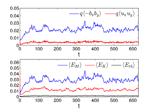
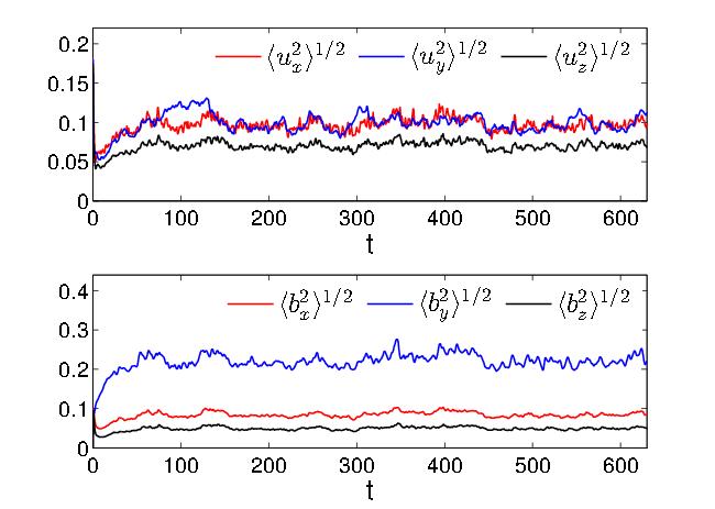
Figure 3: Evolution of volume-averaged Reynolds and Maxwell stresses (top row), kinetic, thermal and magnetic energy densities (second row), rms of velocity (third row) and magnetic field (bottom row) components for the fiducial box $(4,4,1)$. Turbulence sets in after several orbits, with the magnetic energy dominating kinetic and thermal energies, and the Maxwell stress the Reynolds one. The azimuthal component of the turbulent magnetic field is larger than the other two ones due to the shear. It is also about twice larger than the mean field $B_{0y}=0.1$ (Table 1).

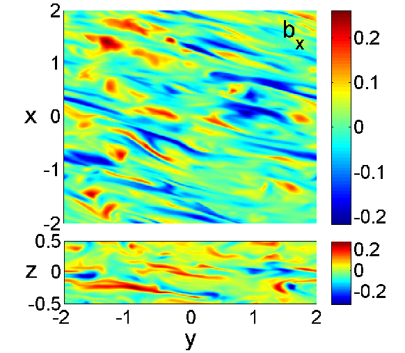
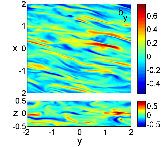
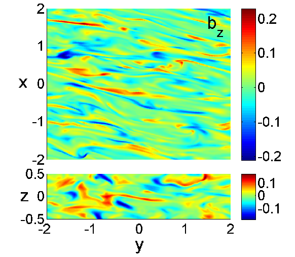
Figure 4: Typical structure of the magnetic field in the fully developed quasi-steady turbulent state at $t=550$ for the box $(4,4,1)$. Shown are the sections in $(y,x)$ and $(y,z)$-planes.

In all the boxes, initially imposed small perturbations start to grow as a result of the nonmodal MRI amplification of the constituent Fourier modes. Then, after several orbits, the perturbation amplitude becomes high enough, reaching the nonlinear regime and eventually the flow settles down into a quasi-steady sustained MHD turbulence. Figure 3 shows the time-development of the volume-averaged perturbed kinetic, $\langle E_{K}\rangle$, thermal, $\langle E_{th}\rangle$, and magnetic, $\langle E_{M}\rangle$, energy densities as well as the Reynolds, $\langle u_{x}u_{y}\rangle$, and Maxwell $-\langle b_{x}b_{y}\rangle$ stresses for the fiducial box $(4,4,1)$. For completeness, in this figure, we also show the evolution of the rms values of the turbulent velocity and magnetic field components. The magnetic energy dominates the kinetic and thermal ones, with the latter being much smaller than the former two, while the Maxwell stress is about 5 times larger than the Reynolds one. This indicates that the magnetic field perturbations are primarily responsible for energy extraction from the mean flow by the Maxwell stress, transporting angular momentum outward and sustaining turbulence. In contrast to the 2D plane case (Mamatsashvili et al., 2014), the Reynolds stress in this 3D case is positive and also contributes to the outward transport. The temporal behavior of the volume-averaged kinetic and magnetic energy densities and stresses is consistent with analogous studies of MRI-turbulence in disks with a net azimuthal field (Hawley et al., 1995; Guan et al., 2009; Simon & Hawley, 2009; Meheut et al., 2015). For all the models, the time- and volume-averaged quantities over the whole quasi-steady state, between $t=100$ and the end of the run at $t_{f}$, are listed in Table 1. For the fiducial model, the ratios of the magnetic energy to kinetic and thermal ones are $\langle\langle E_{M}\rangle\rangle/\langle\langle E_{K}\rangle\rangle=2.4$ and $\langle\langle E_{M}\rangle\rangle/\langle\langle E_{th}\rangle\rangle=15.8$, respectively, and the ratio of the Maxwell stress to the Reynolds stress is $\langle\langle-b_{x}b_{y}\rangle\rangle/\langle\langle u_{x}u_{y}\rangle\rangle=5.21$. For other boxes, similar ratios hold between magnetic and hydrodynamic quantities, as can be read off from Table 1, with the magnetic energy and stresses being always dominant over respective hydrodynamic ones. Interestingly, for all boxes in the quasi-steady turbulent state, $\langle E_{M}\rangle$ and $\langle-b_{x}b_{y}\rangle$ closely follow each other at all times, with the ratio being nearly constant, $\langle E_{M}\rangle/\langle-b_{x}b_{y}\rangle\approx 2$ (see also Hawley et al., 1995; Guan et al., 2009). From Table 1, we can also see how the level (intensity) of the turbulence varies with the radial and azimuthal sizes of the boxes. For fixed $L_{y}=4$, the saturated values of the energies and stresses increase with $L_{x}$, but only very little, so they can be considered as nearly unchanged, especially after $L_{x}>1$. By contrast, at fixed $L_{x}=4$, these quantities are more sensitive to the azimuthal size $L_{y}$, increasing more than twice with the increase of the latter from $L_{y}=2$ to $L_{y}=4$. However, after $L_{y}=4$ the increase of the turbulence strength with the box size is slower, as evident from the box $(8,8,1)$. This type of dependence of the azimuthal MRI-turbulence characteristics on the horizontal sizes of the simulation box is consistent with that of Guan et al. (2009).

The structure of the turbulent magnetic field in the fully developed quasi-steady turbulence in physical space is presented in Figure 4. It is chaotic and stretched along the $y$-axis due to the shear, with $b_{y}$ achieving higher values than $b_{x}$ and $b_{z}$. At this moment, the rms values of these components are, $\langle b_{x}^{2}\rangle^{1/2}=0.079$, $\langle b_{z}^{2}\rangle^{1/2}=0.044$, while $\langle b_{y}^{2}\rangle^{1/2}=0.2$ and is twice larger than the background field $B_{0y}=0.1$. These values, as expected, are consistent with the bottom panel of Figure 3. So, the turbulent field satisfies $\langle b_{z}^{2}\rangle^{1/2}<\langle b_{x}^{2}\rangle^{1/2}<B_{0y}<\langle b_{y}^{2}\rangle^{1/2}$, which in fact holds throughout the evolution for all models (Table 1).

4.1 Analysis in Fourier space – an overview

A deeper insight into the nature of the turbulence driven by the azimuthal MRI can be gained by performing analysis in Fourier space. So, following Horton et al. (2010); Mamatsashvili et al. (2014, 2016), we examine in detail the specific spectra and sustaining dynamics of the quasi-steady turbulent state by explicitly calculating and visualizing the individual linear and nonlinear terms in spectral Equations (11)-(17), which have been classified and described in Section 2, based on the simulation data. These equations govern the evolution of the quadratic forms (squared amplitudes) of Fourier transforms of velocity, thermal and magnetic field perturbations and are more informative than Equations (18) and (19) for spectral kinetic and magnetic energies. In the latter equations a lot of essential information is averaged and lost. Therefore, energy equations alone are insufficient for understanding intertwined linear and nonlinear processes that underlie the sustaining dynamics of the turbulence. For this reason, we rely largely on Equations (11)-(17), enabling us to form a complete picture of the turbulence dynamics. So, we divide our analysis in Fourier space into several steps:

1. Three-dimensionality, of course, complicates the analysis. Therefore, initially, we find out which vertical wavenumbers are important by integrating the spectral energies and stresses in $(k_{x},k_{y})$-plane (Figure 5). As will be evident from such analysis, mostly the lower vertical harmonics, $|k_{z}|=0,1,2$, (i.e., with vertical scales comparable to the box size $L_{z}$) engage in the turbulence maintaining process.

2. Next, concentrating on these modes with lower vertical wavenumber, we present the spectral magnetic energy in $(k_{x},k_{y})$-plane (Figure 6) and identify the energy-carrying modes in this plane (Figure 7). From these modes, we delineate a narrower set of dynamically important active ones, which are central in the sustenance process. Based on this, we identify a region in Fourier space – the vital area – where the basic linear and nonlinear processes for these modes operate. Despite a limited extent of the vital area, the number of the dynamically important modes within it appears to be quite large and they are distributed anisotropically in Fourier space.

3. Integrating in $(k_{x},k_{y})$-plane the quadratic forms of the spectral velocity and magnetic field components (${|\bar{u}_{i}|^{2}}$ and ${|\bar{b}_{i}|^{2}}$) as well as the corresponding linear and nonlinear terms on the rhs of Equations 11-17), we obtain a first idea about the importance of each of them in the dynamics as a function of $k_{z}$ (Figure 8). Note that the action of the linear drift terms vanishes after the integration. Nevertheless, the universality and importance of the linear drift is obvious in any case.

4. Finally, we analyze the interplay of these processes/terms that determines the turbulence dynamics (Figures 9-14). As a result, we construct the turbulence sustaining picture/mechanism by revealing the transverse nature of the nonlinear processes – the nonlinear transverse cascade – and demonstrating its key role in the sustenance.

Fromang & Papaloizou (2007); Simon et al. (2009); Davis et al. (2010); Lesur & Longaretti (2011) took a similar approach of representing the MHD equations in Fourier space and analyzing individual linear and nonlinear (transfer) terms in the dynamics of MRI-turbulence. They derived evolution equations for the kinetic and magnetic energy spectra, which are similar to our Equations (18)-(19) except for notation and mean field direction. As mentioned above, we do not make the shell-averages in Fourier space, as done in these studies, that completely wipes out spectral anisotropy due to the shear crucial to the turbulence dynamics.

Since our analysis primarily focuses on the spectral aspect of the dynamics, the SNOOPY code, being of spectral type, is particularly convenient for this purpose, as it allows us to directly extract Fourier transforms. From now on we consider the evolution after the quasi-steady turbulence has set in, so all the spectral quantities/terms in Equations (11)-(17) are averaged in time over an entire saturated turbulent state between $t=200$ and the end of the run. Below we concentrate on the fiducial box $(4,4,1)$. Comparison of the spectral dynamics in other boxes and the effects of the box aspect ratio will be presented in the next Section.

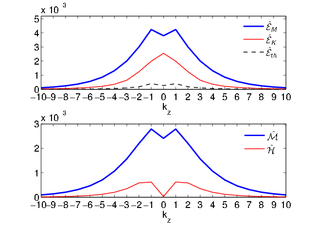
Figure 5: Integrated in $(k_{x},k_{y})$-plane time-averaged kinetic, $\hat{\cal E}_{K}$, magnetic, $\hat{\cal E}_{M}$ and thermal $\hat{\cal E}_{th}$ energy spectra (upper panel) as well as Reynolds, $\hat{\cal H}$, and Maxwell, $\hat{\cal M}$, stresses (lower panel) as a function of $k_{z}$ for the box $(4,4,1)$.

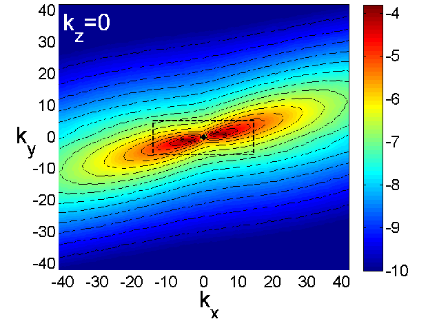
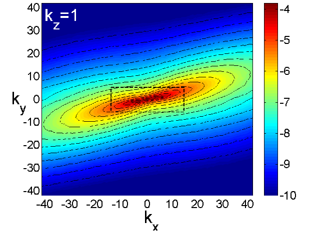
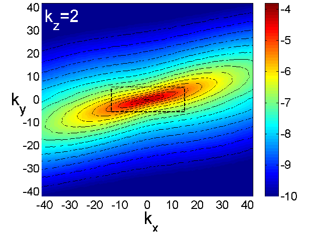
Figure 6: Logarithm of the spectral magnetic energy, $log_{10}{\cal E}_{M}$, in $(k_{x},k_{y})$-plane at $k_{z}=0,1,2$ for the box $(4,4,1)$. The spectra is strongly anisotropic due to the shear, having larger power on the $k_{x}/k_{y}>0$ side at a given $k_{y}$. Dashed rectangles delineate the vital area of turbulence, where the sustaining process is concentrated (see Figures 9-14).

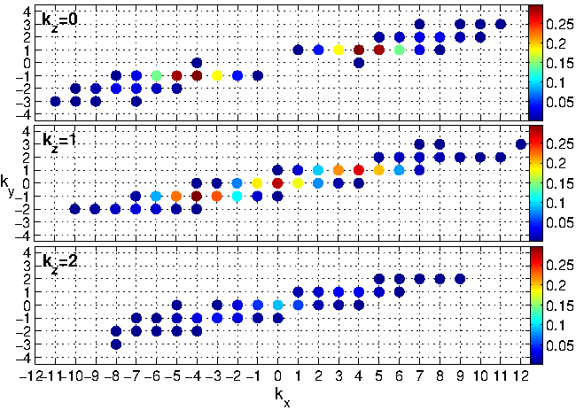
Figure 7: Distribution of the active modes in k-space at $k_{z}=0,1,2$ for the box $(4,4,1)$. The color dots represent the modes whose magnetic energy, ${\cal E}_{M}$, grows more than $50\%$ of the maximum spectral magnetic energy, ${\cal E}_{M,max}$, and the colors indicate the fraction of time each mode contains this higher energy during the quasi-steady state until the end of the simulation.

4.2 Energy spectra, active modes and the vital area

Figure 5 shows the time-averaged spectra of the kinetic, magnetic and thermal energies as well as the Reynolds and Maxwell stresses integrated in $(k_{x},k_{y})$-plane, $\hat{\cal E}_{K,M,th}(k_{z})=\int{\cal E}_{K,M,th}dk_{x}dk_{y}$ and $(\hat{\cal H}(k_{z}),\hat{\cal M}(k_{z}))=\int({\cal H},{\cal M})dk_{x}dk_{y}$ as a function of $k_{z}$. The magnetic energy is the largest and the thermal energy the smallest, while the Maxwell stress dominates the Reynolds one, at all $k_{z}$. All the three energy spectra and stresses reach a maximum at small $|k_{z}|$ – the magnetic and thermal energies as well as the stresses at $|k_{z}|=1$, while the kinetic energy at $k_{z}=0$ – and rapidly decrease with increasing $|k_{z}|$. As a result, in particular, the magnetic energy injection into turbulence due to the Maxwell stress takes place mostly at small $k_{z}$, which is consistent with our linear optimal growth calculations (Section 3) and also with Squire & Bhattacharjee (2014), but is in contrast to the accepted view that the purely azimuthal field MRI is stronger at high $k_{z}$ (Balbus & Hawley, 1992; Hawley et al., 1995). The main reason for this difference, as mentioned above, is that the latter is usually calculated over much longer times (spanning from tens to hundred dynamical times), following the evolution of the shearing waves from initial tightly leading to final tightly trailing orientation, whereas the optimal growth is usually calculated over a finite (dynamical) time, which seems more appropriate in the case of turbulence. Thus, the large-scale modes with the first few $k_{z}$ contain most of the energy and hence play a dynamically important role.

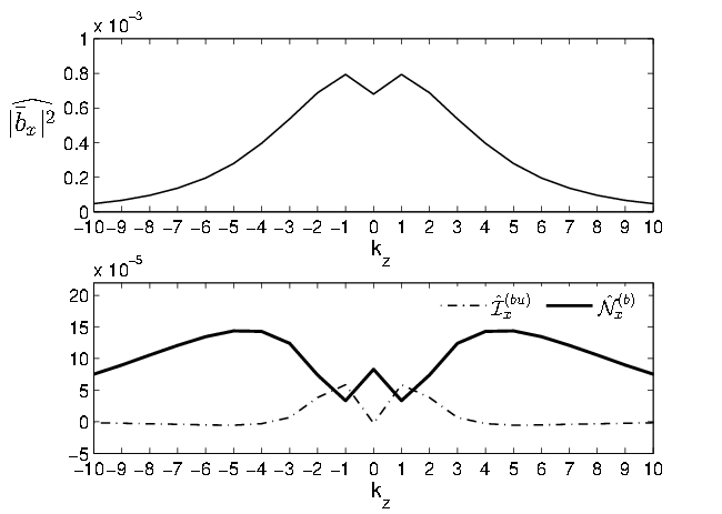
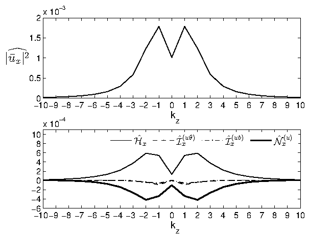
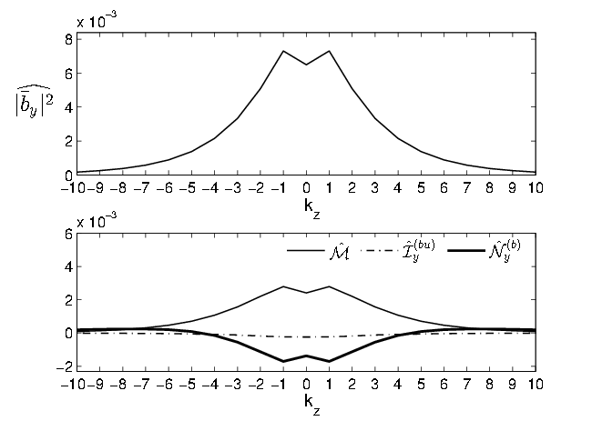
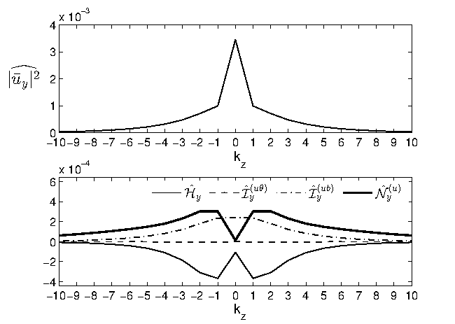
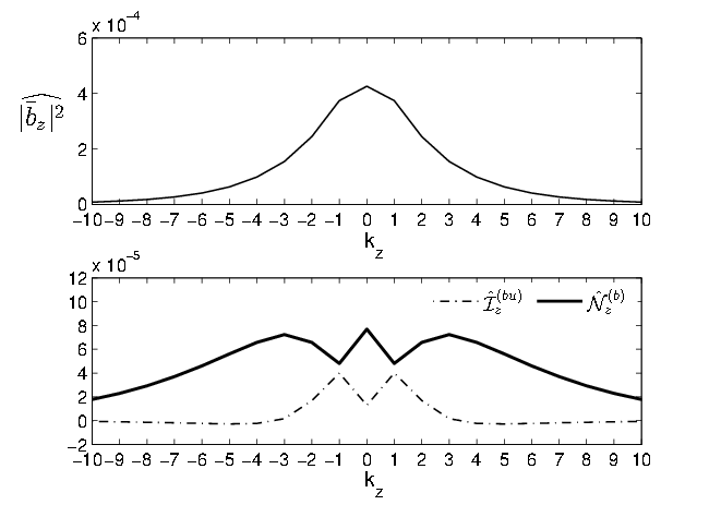
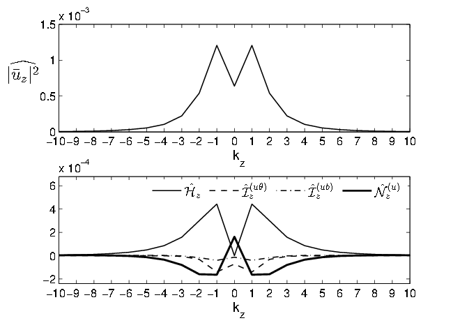
Figure 8: Integrated in $(k_{x},k_{y})$-plane the quadratic forms of the spectral velocity and magnetic field components together with the corresponding linear and nonlinear terms from corresponding Equations (11)-(17) as a function of $k_{z}$.

To have a fuller picture of the energy spectra, in Figure 6 we present sections of ${\cal E}_{M}$ in $(k_{x},k_{y})$-plane again at first three vertical wavenumbers $k_{z}=0,1,2$, for which it is higher (see Figure 5). The spectrum is highly anisotropic due to the shear with the same elliptical shape and inclination towards the $k_{x}-$axis irrespective of $k_{z}$. This indicates that modes with $k_{x}/k_{y}>0$ have more energy than those with $k_{x}/k_{y}<0$ at fixed $k_{y}$. The kinetic energy spectrum shares similar properties and is not shown here. A similar anisotropic spectrum was already reported in the shearing-box simulations of MRI-turbulence with a nonzero net vertical field (Hawley et al., 1995; Lesur & Longaretti, 2011; Murphy & Pessah, 2015). This energy spectrum, which clearly differs from a typical turbulent spectrum in the classical case of forced MHD turbulence without shear (Biskamp, 2003), arises as a consequence of a specific anisotropy of the linear and nonlinear terms of Equations (11)-(17) in ${\bf k}-$space. These new features are not common to shearless MHD turbulence and hence it is not surprising that Kolmogorov or IK theory cannot adequately describe shear flow turbulence.

Having described the energy spectrum, we now look at how energy-carrying modes, most actively participating in the dynamics, are distributed in $(k_{x},k_{y})$-plane. We refer to modes whose magnetic energy reaches values higher than 50% of the maximum spectral magnetic energy as active modes. Although this definition is somewhat arbitrary, it gives an idea on where the dynamically important modes are located in Fourier space. Figure 7 shows these modes in $(k_{x},k_{y})$-plane at $k_{z}=0,1,2$ with color dots. They are obtained by following the evolution of all the modes in the box during an entire quasi-steady state and selecting those modes whose magnetic energy becomes higher than the above threshold. The color of each mode indicates the fraction of time, from the onset of the quasi-steady state till the end of the simulation, during which it contains this higher energy. We have also checked that Figure 7 is not qualitatively affected upon changing the 50% threshold to either 20% or 70%. Like the energy spectrum, the active modes with different duration of “activity” are distributed quite anisotropically in $(k_{x},k_{y})$-plane, occupying a broader range of radial wavenumbers $|k_{x}|\lesssim 12$ than that of azimuthal ones $|k_{y}|\lesssim 3$. This main, energy-containing area in k-space represents the vital area of turbulence. Essentially, the active modes in the vital area take part in the sustaining dynamics of turbulence. The other modes with larger wavenumbers lie outside the vital area and always have energies and stresses less than 50% of the maximum value, therefore, not playing as much a role in the energy-exchange process between the background flow and turbulence. Note that the total number of the active modes (color dots) in Figure 7 is equal to $114$, implying that the dynamics of the MRI-turbulence, strictly speaking, cannot be reduced to low-order models of the sustaining processes, involving only a small number of active modes (e.g., Herault et al., 2011; Riols et al., 2017).

4.3 Vertical spectra of the dynamical terms

Having identified the vital area, we now examine the significance of each of the linear and nonlinear terms in this area first along the vertical $k_{z}$-direction in Fourier space. For this purpose, we integrate in $(k_{x},k_{y})$-plane the quadratic forms of the spectral velocity and magnetic field components as well as the rhs terms of Equations (11)-(13) and (15)-(17), as we have done for the spectral energies and stresses above. We do not apply this procedure to the linear drift term (which vanishes after such integration) and dissipation terms, as their action is well known. The results are presented in Figure 8 (the spectral quantities integrated in $(k_{x},k_{y})$-plane are all denoted by hats), which shows that:

1. The dynamics of $\widehat{|\bar{b}_{x}|^{2}}$ is governed by $\hat{\cal I}_{x}^{(bu)}$ and $\hat{\cal N}^{(b)}_{x}$, which are both positive and therefore act as a source for the radial field at all $k_{z}$.

2. The dynamics of $\widehat{|\bar{b}_{y}|^{2}}$ is governed by $\hat{\cal M}$ and $\hat{\cal N}^{(b)}_{y}$, the action of $\hat{\cal I}_{y}^{(bu)}$ is negligible compared with these terms. The effect of $\hat{\cal M}$ is positive for all $k_{z}$, reaching a maximum, as we have seen before, at $|k_{z}|=1$. This implies that the energy injection into turbulence from the background flow due to the MRI occurs over a range of length scales, preventing the development of the proper inertial range in the classical sense (see also Lesur & Longaretti, 2011). On the other hand, $\hat{\cal N}^{(b)}_{y}$ is negative and hence acts as a sink for low/active $k_{z}$, but positive at large $|k_{z}|$. So, the nonlinear term transfers the azimuthal field component from these wavenumbers to large $|k_{z}|$ as well as (which is more important) to other components.

3. The dynamics of $\widehat{|\bar{b}_{z}|^{2}}$ is governed by $\hat{\cal I}_{z}^{(bu)}$ and $\hat{\cal N}^{(b)}_{z}$, which are both positive, with the latter being larger than the former at all $k_{z}$. Note that $\widehat{|\bar{b}_{z}|^{2}}$ is smaller compared to the other two components, while $\widehat{|\bar{b}_{y}|^{2}}$ is the largest.

4. The dynamics of $\widehat{|\bar{u}_{x}|^{2}}$ is governed by $\hat{\cal H}_{x}$ and $\hat{\cal N}^{(u)}_{x}$, the action of the exchange terms, $\hat{\cal I}_{x}^{(u\theta)}$ and $\hat{\cal I}_{x}^{(ub)}$, are negligible compared to these terms. The effect of $\hat{\cal H}_{x}$ is positive for all $k_{z}$, acting as the only source for $\bar{u}_{x}$. By contrast, $\hat{\cal N}^{(u)}_{x}$ is negative (sink), opposing $\hat{\cal H}_{x}$, with a similar dependence of its absolute value on $k_{z}$. So, the nonlinear term transfers the radial velocity to other components.

5. The dynamics of $\widehat{|\bar{u}_{y}|^{2}}$ is governed by $\hat{\cal H}_{y}$, $\hat{\cal I}_{y}^{(ub)}$ and $\hat{\cal N}^{(u)}_{y}$, the action of $\hat{\cal I}_{y}^{(u\theta)}$ is negligible. The effects of $\hat{\cal N}^{(u)}_{y}$ and $\hat{\cal I}_{y}^{(ub)}$ are positive for all $k_{z}$, while $\hat{\cal H}_{y}$ is negative. Special attention deserves the sharp peak of $\widehat{|\bar{u}_{y}|^{2}}$ at $k_{z}=0$. This peak is related to the formation of the zonal flow with $|k_{x}|=1$ and $k_{y}=0$ in the MRI-turbulence (Johansen et al., 2009), which will be analyzed below.

6. The dynamics of $\widehat{|\bar{u}_{z}|^{2}}$ is governed by $\hat{\cal H}_{z}$, $\hat{\cal I}_{z}^{(u\theta)}$ and $\hat{\cal N}^{(u)}_{z}$, the action of $\hat{\cal I}_{z}^{(ub)}$ is negligible. $\widehat{|\bar{u}_{z}|^{2}}$ is the only term that explicitly depends on the thermal processes. Note also that $\hat{\cal N}^{(u)}_{z}$ is negative at $|k_{z}|\geq 1$, but becomes positive at $k_{z}=0$, implying inverse transfer towards small $k_{z}$. We do not go into the details of this dependence, as $\widehat{|\bar{u}_{z}|^{2}}$ is anyway smaller compared to the other components. Besides, the thermal processes do not play a major role in the overall dynamics, since their energy is much smaller than the magnetic end kinetic energies (see also Figure 3).

It is seen from Figure 8 that all the dynamical terms primarily operate at small vertical wavenumbers $|k_{z}|=0,1,2$. Some of them ($\hat{\cal N}_{x}^{(b)}$ and $\hat{\cal N}_{z}^{(b)}$) may extend up to $|k_{z}|=3-6$, but eventually decay at large $|k_{z}|$. Similarly, the spectra of the velocity and magnetic field have relatively large values also at small $|k_{z}|$. So, $|k_{z}|=2$ can be viewed as an upper vertical boundary of the vital area in Fourier space.

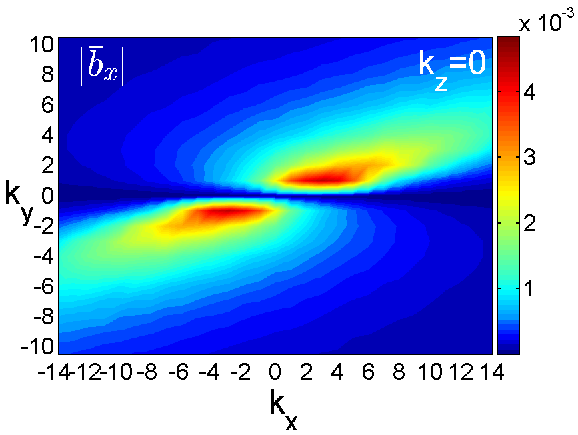
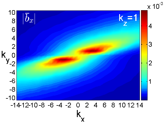
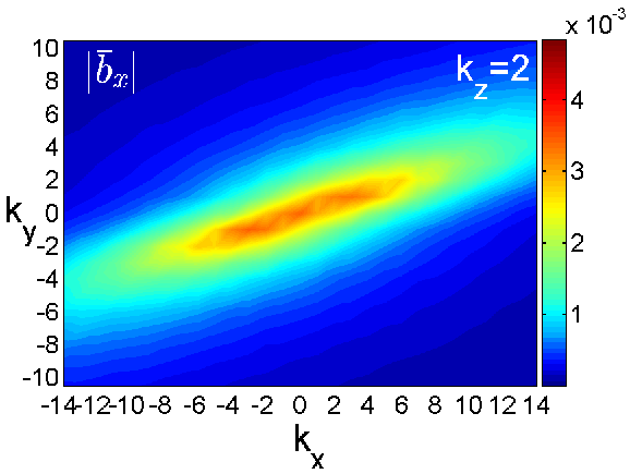
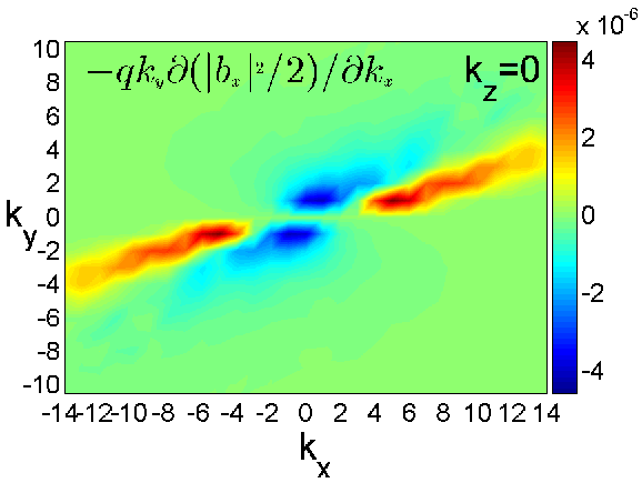
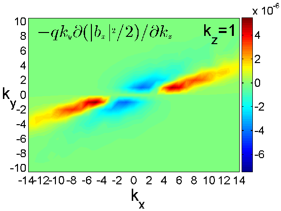
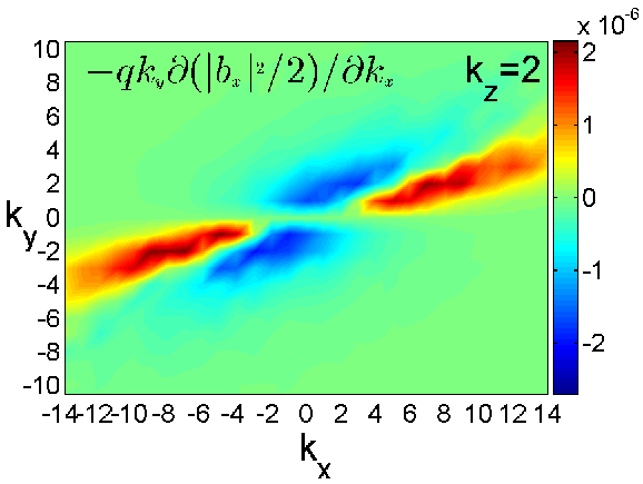
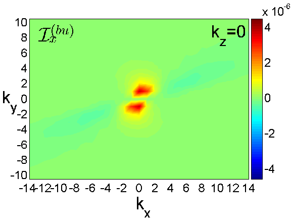
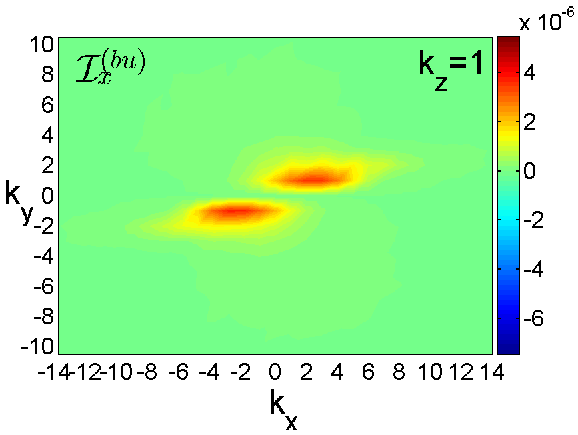
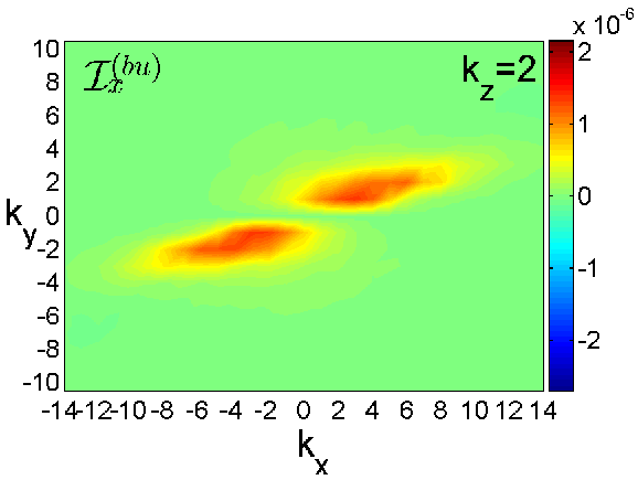
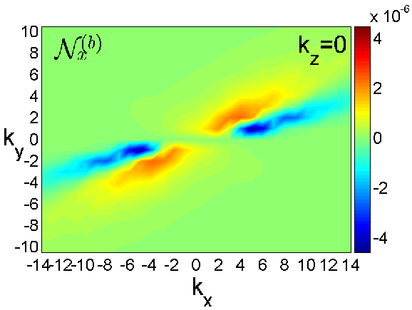
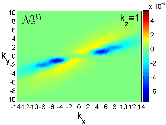
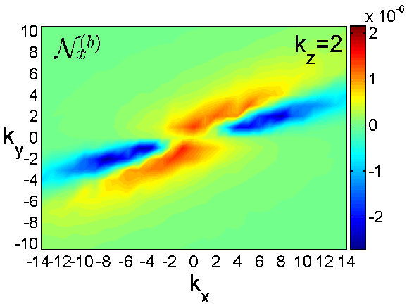
Figure 9: Spectrum of the radial field, $|\bar{b}_{x}|$, and the maps of the corresponding linear and nonlinear terms, governing its dynamics (Equation 15), in $(k_{x},k_{y})$-plane at $k_{z}=0(left),~{}1(middle),~{}2(right)$. The spectrum as well as the action of these terms are highly anisotropic, (i.e., depend on the wavevector azimuthal angle) due to the shear. These terms are appreciable and primarily operate in the vital area $|k_{x}|\lesssim 12,|k_{y}|\lesssim 3$. The red and yellow (blue and dark blue) regions in each panel correspond to wavenumbers where respective dynamical terms are positive (negative) and hence act as a source (sink) for $|\bar{b}_{x}|^{2}$. In light green regions, outside the vital area, these terms are small, although, as we checked, preserve the same anisotropic shape. In particular, the nonlinear transfer term ${\cal N}_{x}^{(b)}$ transversely redistributes $|\bar{b}_{x}|^{2}$ from the blue and dark blue regions, where ${\cal N}_{x}^{(b)}<0$, to the red and yellow regions, where ${\cal N}_{x}^{(b)}>0$. These regions exhibit considerable variations with the azimuthal angle of the wavevector and also depend on $k_{z}$.

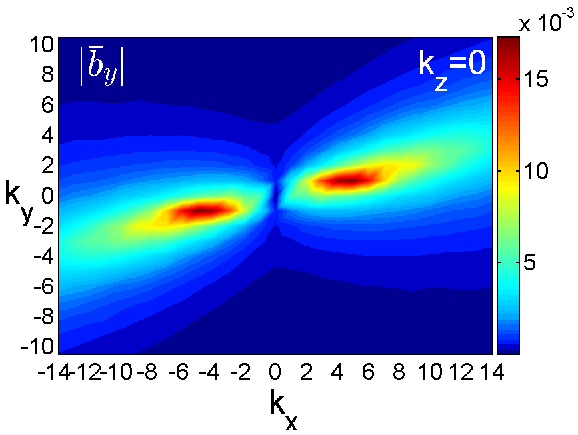
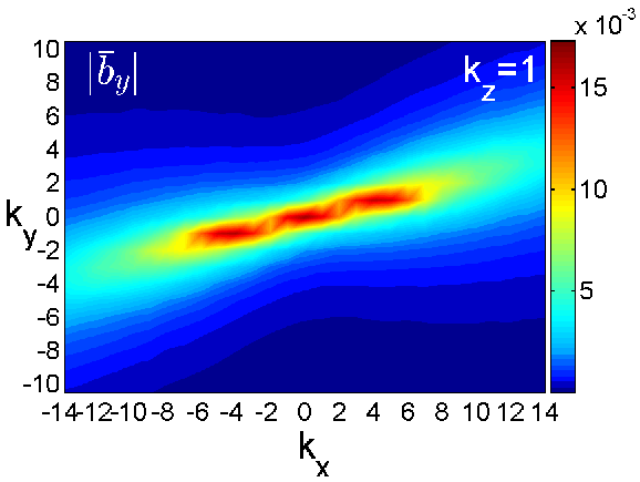
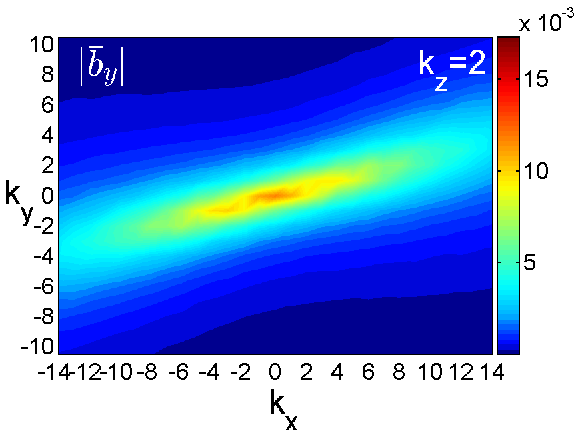
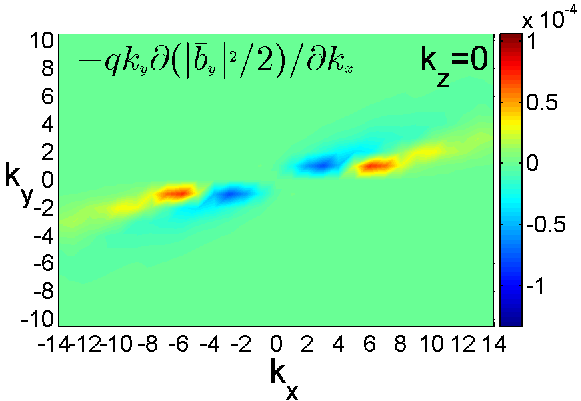
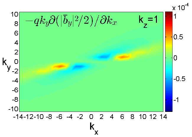
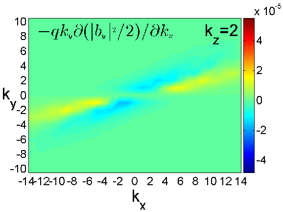
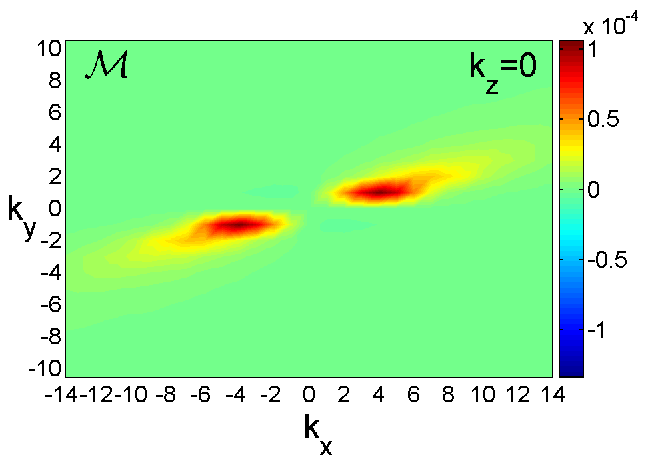
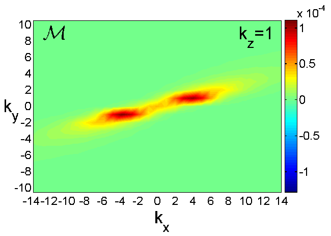
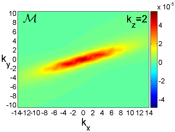
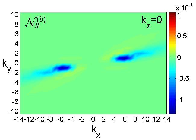
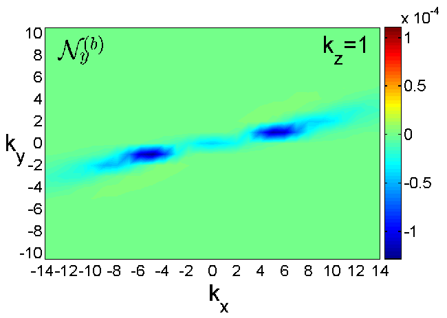
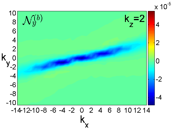
Figure 10: Same as in Figure 9, but for the azimuthal field $\bar{b}_{y}$ with the corresponding dynamical terms from Equation (16). The dynamics of this component is primarily determined by the combined action of the drift, the Maxwell stress ${\cal M}$, which is positive (energy injection) and the nonlinear term ${\cal N}_{y}^{(b)}$, which is negative (sink) in the vital area. The linear exchange term ${\cal I}_{y}^{(bu)}$ is negligible compared with the above terms and is not shown here.

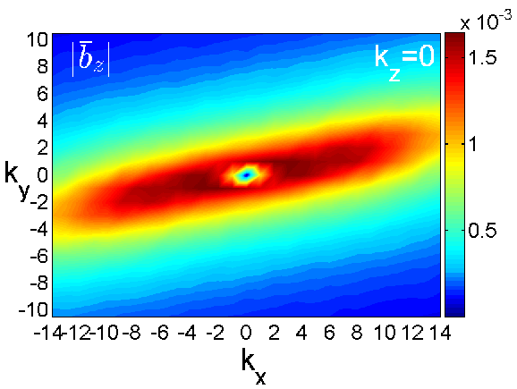
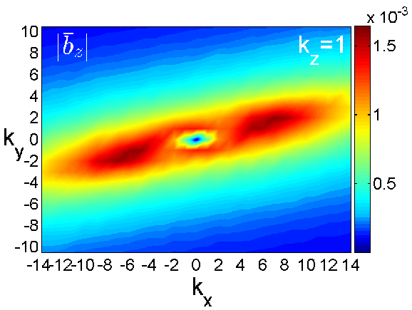
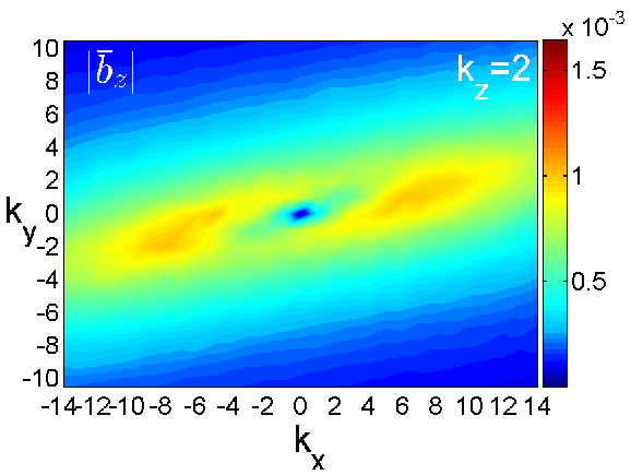
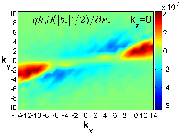
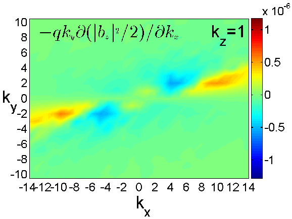
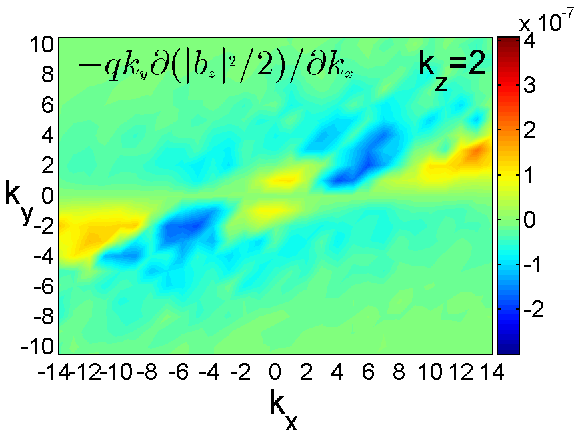
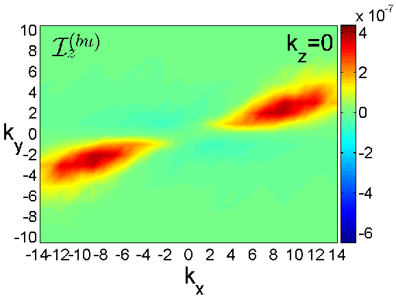
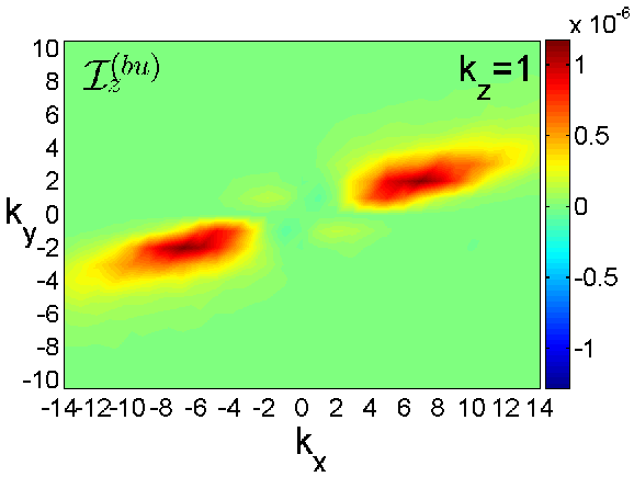
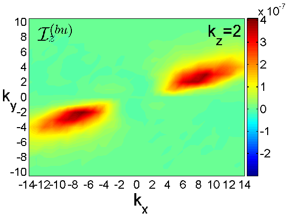
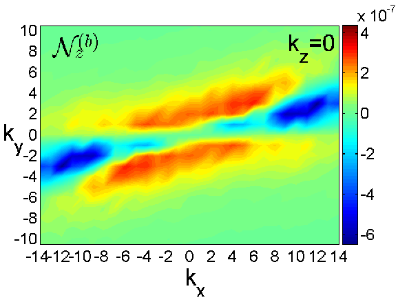
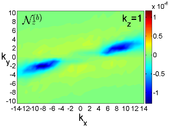
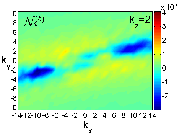
Figure 11: Same as in Figure 9, but for $\bar{b}_{z}$ with the corresponding dynamical terms from Equation (17). The transverse character of the nonlinear redistribution, ${\cal N}_{z}^{(b)}$, is also evident. $|\bar{b}_{z}|$ is small in comparison with $|\bar{b}_{x}|$ and $|\bar{b}_{y}|$.

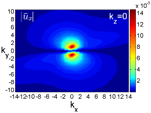
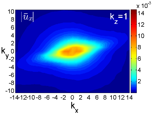
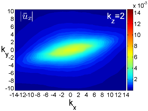
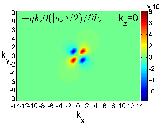
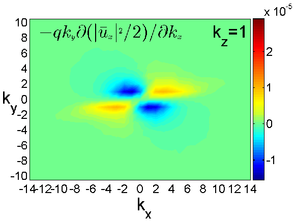
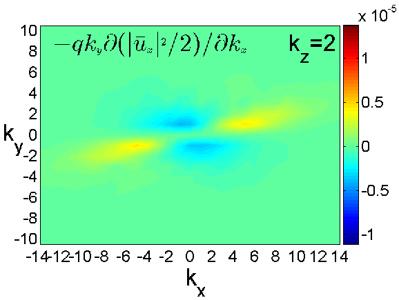
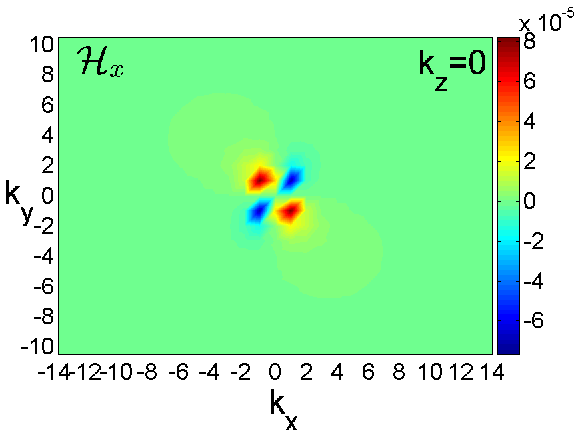
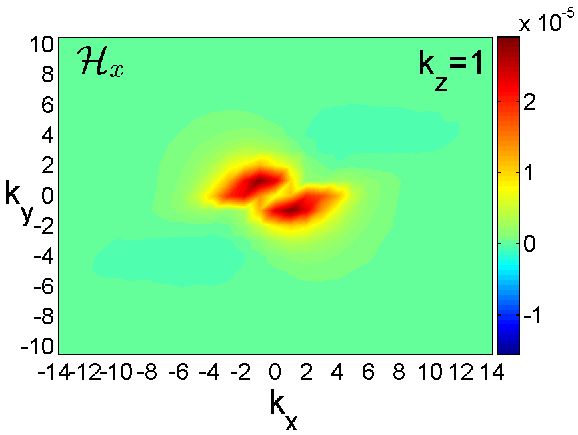
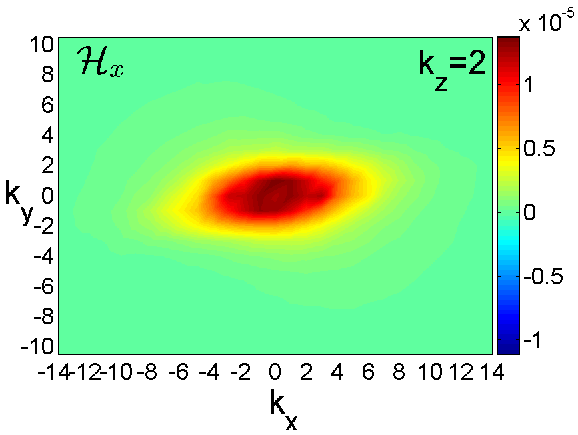
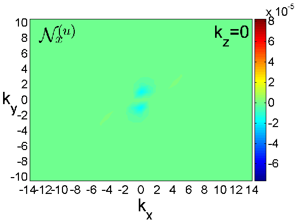
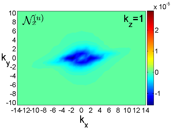
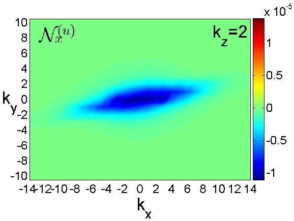
Figure 12: Spectra of $|\bar{u}_{x}|$ and the maps of the corresponding linear and nonlinear terms governing its dynamics (Equation 11) in $(k_{x},k_{y})$-plane at $k_{z}=0(left),1(middle),2(right)$. The dynamics of this velocity component is primarily determined by ${\cal H}_{x}$ (source) and ${\cal N}_{x}^{(u)}$ (sink), the linear exchange terms, ${\cal I}_{x}^{(u\theta)}$ and ${\cal I}_{x}^{(ub)}$, are negligible compared with the above terms and are not shown here.

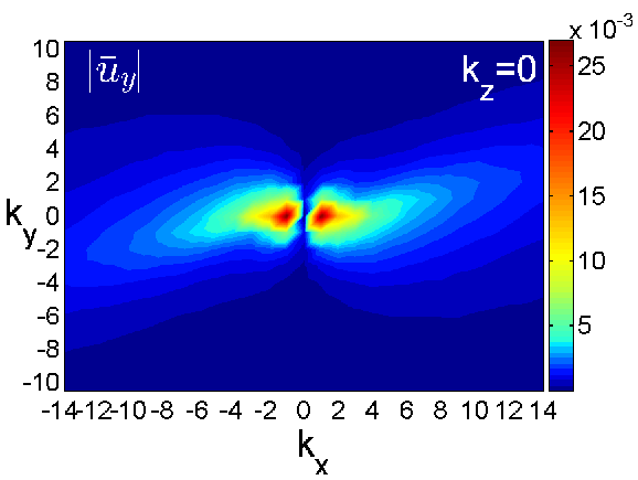
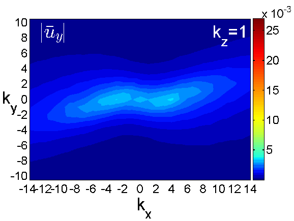
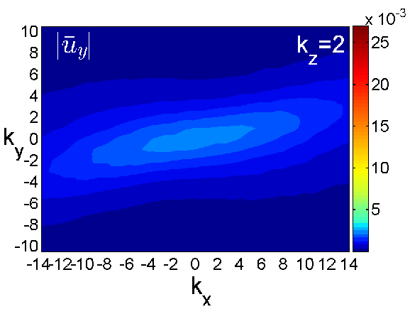
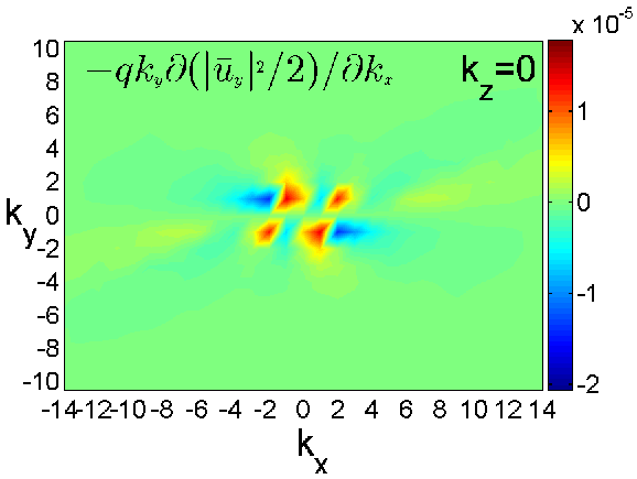
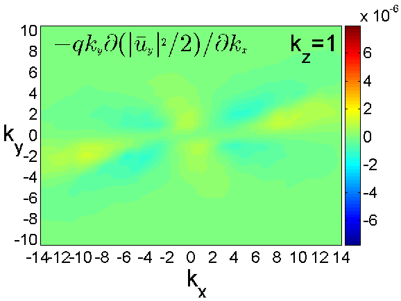
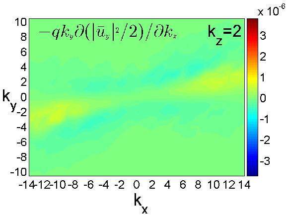
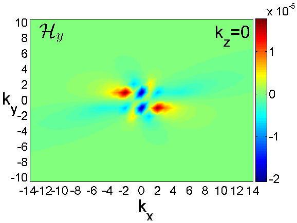
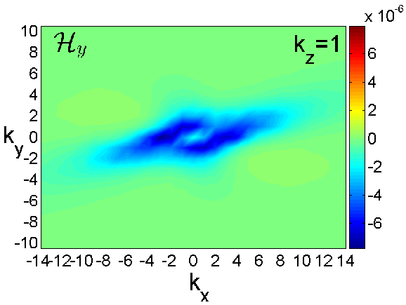
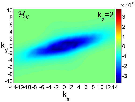
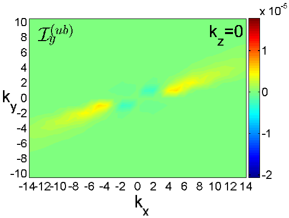
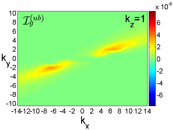
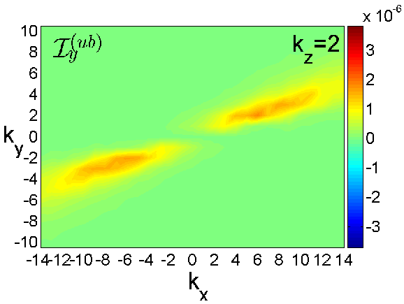
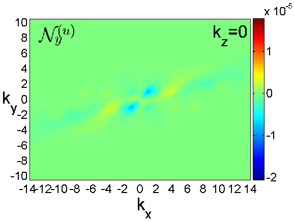
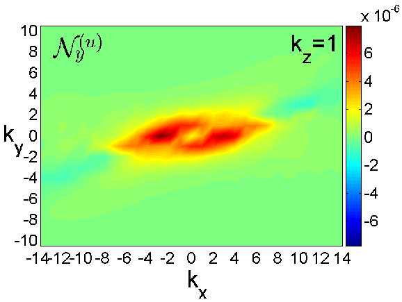
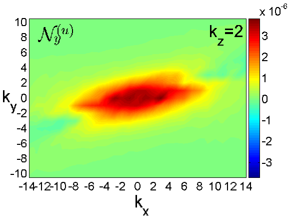
Figure 13: Same as in Figure 12, but for $\bar{u}_{y}$ with the corresponding dynamical terms from Equation (12). The influence of the thermal process, ${\cal I}_{y}^{(u\theta)}$, is negligible and not shown here. The spectrum of $|\bar{u}_{y}|$ reaches a maximum at $k_{x}=\pm 1,k_{y}=k_{z}=0$, which corresponds to the zonal flow in physical space.

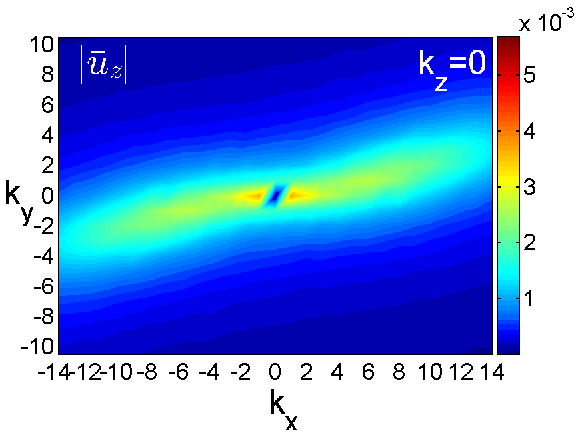
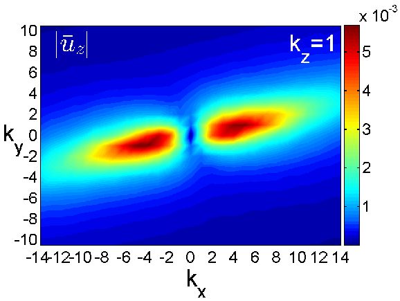
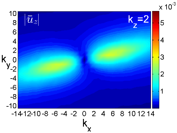
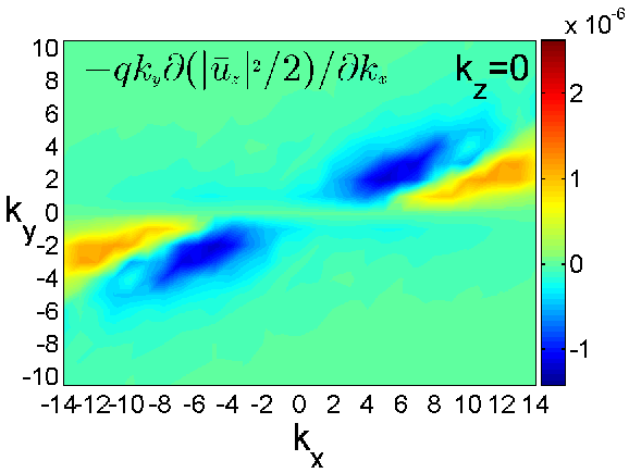
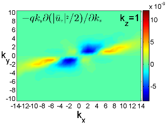
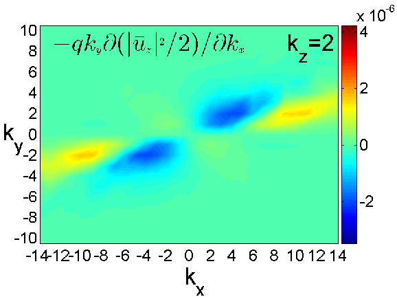
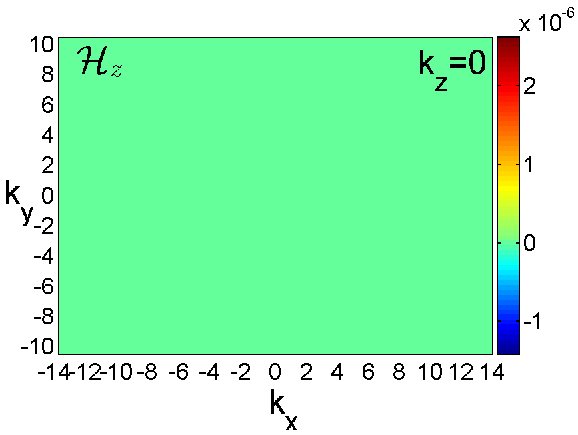
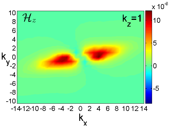
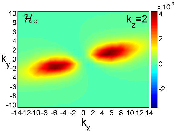
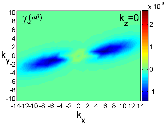
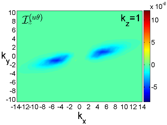
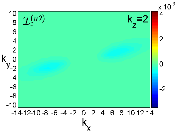
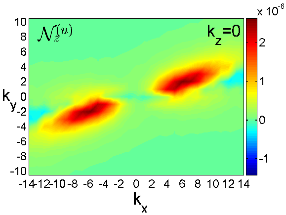
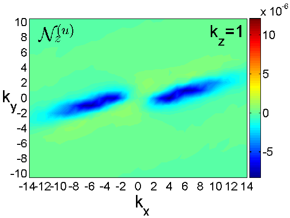
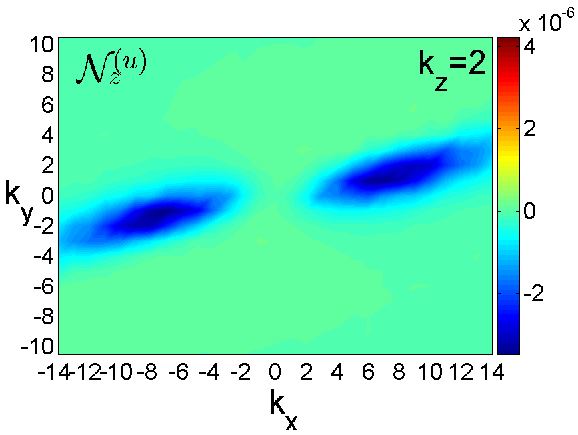
Figure 14: Same as in Figure 12, but for $\bar{u}_{z}$ with the corresponding dynamical terms from Equation (13). The influence of the linear magnetic exchange term ${\cal I}_{z}^{(ub)}$ is negligible and is not shown here. The nonlinear term ${\cal N}_{z}^{(u)}$ transfers $|\bar{u}_{z}|^{2}$ towards small $k_{z}$ (as it also seen in the corresponding panel of Figure 8).

5 Interplay of the linear and nonlinear processes in the sustenance of the turbulence

We have seen above that the sustaining dynamics of turbulence is primarily concentrated at small vertical wavenumbers, so now we present the distribution of the time-averaged amplitudes of the spectral quantities $\bar{u}_{i}$, $\bar{b}_{i}$ as well as the linear ($k_{x}$-drift, ${\cal H}_{i},{\cal I}_{i},{\cal M}$) and nonlinear (${\cal N}_{i}$) dynamical terms in $(k_{x},k_{y})$-plane again at $k_{z}=0,1,2$ in Figures 9-14 (as noted before, we omit here the thermal processes, $\bar{\theta}$, which play a minor role). These figures give quite a detailed information and insight about all the linear and nonlinear processes involved in Equations (11)-(17) and allow us to properly understand their interplay leading to the turbulence sustenance. We start the analysis of this interplay with a general outline of the figures. We do not show here the viscous (${\cal D}_{i}^{(u)}$) and resistive ${\cal D}_{i}^{(b)}$ terms, since their action is quite simple – they are always negative and reduce the corresponding quantities, thereby opposing the sustenance process. They increase with $k$, but in the vital area are too small to have any influence on the dynamics.

A first glance at the plots makes it clear that all the spectra of the physical quantities and processes are highly anisotropic due to the shear, i.e., strongly depend on the azimuthal angle in $(k_{x},k_{y})$-planes as well as vary with $k_{z}$, with a similar type of anisotropy and inclination towards the $k_{x}$-axis, as the energy spectrum in Figure 6. For the nonlinear processes represented by ${\cal N}_{i}^{(u)}$ and ${\cal N}_{i}^{(b)}$ (bottom row in Figures 9-14), this anisotropy can not be put within the framework of commonly considered forms of nonlinear – direct and inverse – cascades, since its main manifestation is the transverse (among wavevector angles) nonlinear redistribution of modes in $(k_{x},k_{y})$-plane as well as among different $k_{z}$. In these figures, the nonlinear terms transfer the corresponding quadratic forms of the velocity and magnetic field components transversely away from the regions where they are negative (${\cal N}_{i}^{(u)}<0,{\cal N}_{i}^{(b)}<0$, blue and dark blue) towards the regions where they are positive (${\cal N}_{i}^{(u)}>0,{\cal N}_{i}^{(b)}>0$, yellow and red). These regions display quite a strong angular variation in $(k_{x},k_{y})$-planes.

Similarly, the terms of linear origin ${\cal H}_{i},{\cal I}_{i},{\cal M}$ are strongly anisotropic in $(k_{x},k_{y})$-plane. For the corresponding quantity, they act as a source when positive (red and yellow regions) and as a sink when negative (blue and dark blue regions). The linear exchange of energy with the background shear flow (which is the central energy supply for turbulence) involves all the components of the velocity perturbation through ${\cal H}_{i}$ terms in Equations (11)-(13) and only the azimuthal $y$-component of the magnetic field perturbation through the Maxwell stress term, ${\cal M}$, in Equation (16). However, the other quadratic forms can grow due to the linear exchange, ${\cal I}_{i}$, and nonlinear, ${\cal N}_{i}$, terms. The growth of the quadratic forms and energy extraction from the flow as a result of the operation of all these linear terms essentially constitutes the azimuthal MRI in the flow.

The linear drift parallel to the $k_{x}$-axis is equally important for all the physical quantities. The plots depicting the drift (second row in Figures 9-14), show that this process transfers modes with velocity $|qk_{y}|$ along $k_{x}$-axis at $k_{y}>0$ and in the opposite direction at $k_{y}<0$. Namely, the drift gives the linear growth of individual harmonics a transient nature, as it sweeps them through the vital area in k-space. One has to note that the dynamics of axisymmetric modes with $k_{y}=0$ should be analyzed separately, as the drift does not affect them. Consequently, the drift can not limit the duration of their amplification and if there is any, even weak, linear or nonlinear source of growth at $k_{y}=0$, these harmonics can reach high amplitudes.

Let us turn to the analysis of the route ensuring the turbulence sustenance. First of all, we point out that it should primarily rely on magnetic perturbations, as the Maxwell stress is mainly responsible for energy supply for turbulence. From Figure 9, it is seen that the linear exchange term ${\cal I}_{x}^{(bu)}$ and the nonlinear term ${\cal N}^{(b)}_{x}$ make comparable contributions to the generation and maintenance of the radial field component $|\bar{b}_{x}|$. This is also consistent with the related plots in Figure 8. The exchange term takes energy from the radial velocity $\bar{u}_{x}$ and gives to $\bar{b}_{x}$. The distribution of ${\cal N}^{(b)}_{x}$ clearly demonstrates transversal transfer of $|\bar{b}_{x}|^{2}$ in $(k_{x},k_{y})$-plane for all considered $k_{z}=0,1,2$ as well as among different components. The linear drift term also participates in forming the final spectrum of $|\bar{b}_{x}|$ in the quasi-steady turbulent state. It opposes the action of the nonlinear term: for $k_{y}>0$ ($k_{y}<0$), ${\cal N}_{x}^{(b)}$, transfers modes to the left (right), from the blue and dark blue region to the red and yellow regions, while the drift transfers in the opposite direction. So, the interplay of the drift, ${\cal I}_{x}^{(bu)}$ and ${\cal N}_{x}^{(b)}$ yields the specific anisotropic spectra of $|\bar{b}_{x}|$ shown in the top row of this figure. Particularly noteworthy is the role of the nonlinear term at $k_{y}=0,k_{z}=1,2$, because the drift and the linear magnetic-kinetic exchange terms are proportional to $k_{y}$ and hence vanish. As a result, axisymmetric modes with $k_{y}=0$ are energetically supported only by the nonlinear term. (At $k_{y}=0$, although ${\cal N}_{x}^{(b)}$ is positive both at $k_{z}=1$ and $k_{z}=2$, its values at $k_{z}=1$ are about an order of magnitude smaller than those at $k_{z}=2$ and might not be well represented by light green color in the bottom middle panel in Figure 9.) So, $\bar{b}_{x}$, which is remarkably generated by the nonlinear term, in turn, is a key factor in the production and distribution of the energy-injecting Maxwell stress, ${\cal M}$, in Fourier space. Indeed, note the correlation between the distributions of $|\bar{b}_{x}|$ and ${\cal M}$ in $(k_{x},k_{y})$-plane depicted, respectively, in the top row of Figure 9 and in the third row of Figure 10.

From Figure 10 it is evident that, in fact, the Maxwell stress, ${\cal M}$, which is positive in $(k_{x},k_{y})$-plane and appreciable in the vital area, is the only source for the quadratic form of the azimuthal field component, $|\bar{b}_{y}|^{2}$, and hence for the turbulent magnetic energy, which is dominated by this component. The linear exchange term, ${\cal I}_{y}^{(bu)}$, appears to be much smaller with this stress term (and hence is not shown in this figure). The nonlinear term, ${\cal N}^{(b)}_{y}$, is negative in the vital area (blue regions in the bottom row of Figure 10), draining $|\bar{b}_{y}|^{2}$ there and transferring it to large wavenumbers as well as among different components. Thus, the sustenance of the magnetic energy is of linear origin, due solely to the Maxwell stress that, in turn, is generated from the radial field component. This stage constitutes the main (linear) part of the sustenance scheme, which will be described in the next subsection, and is actually a manifestation of the azimuthal MRI.

The dynamics of the vertical field component $\bar{b}_{z}$ is shown in 11. This components is smaller than $\bar{b}_{x}$ and $\bar{b}_{y}$. The linear exchange term, ${\cal I}_{z}^{(bu)}$, acts as a source, supplying $\bar{b}_{z}$ from the vertical velocity $\bar{u}_{z}$. The nonlinear term, ${\cal N}^{(b)}_{z}$, also realizes the transverse cascade and scatters the modes in different areas of $(k_{x},k_{y})$-plane (from the yellow and red to blue and dark blue areas in the bottom row of Figure 11). However, as it is seen from the related plot in Figure 8, the cumulative effect of ${\cal N}^{(b)}_{z}$ in $(k_{x},k_{y})$-plane is positive and even prevails over the positive cumulative contribution of ${\cal I}_{z}^{(bu)}$ in this plane at every $k_{z}$. As it is clearly seen from Figure 11, the linear drift term opposes the action of the nonlinear term for $\bar{b}_{z}$, similar to that in the case of $\bar{b}_{x}$.

Figure 12 shows that the linear term ${\cal H}_{x}$ can be positive and act as a source for the radial velocity $|\bar{u}_{x}|^{2}$ at the expense of the mean flow, while the nonlinear term ${\cal N}^{(u)}_{x}$ is negative and drains it. The exchange terms ${\cal I}_{x}^{(u\theta)}$, ${\cal I}_{x}^{(ub)}$ are also negative, giving the energy of the radial velocity, respectively, to $\bar{\theta}$ and $\bar{b}_{x}$, but their contributions are negligible compared with ${\cal H}_{x}$ and ${\cal N}_{x}^{(u)}$ and hence not shown in this figure. So, the sustenance of $|\bar{u}_{x}|$ is ensured by the interplay of the linear drift and ${\cal H}_{x}$ terms. Indeed, shifting the result of the action of ${\cal H}_{x}$ by the linear drift to the right (left) for $k_{y}>0$ ($k_{y}<0$) gives the spectrum of $|\bar{u}_{x}|$ presented in the top row this figure.

Figure 13 shows that the dynamics of the azimuthal velocity $\bar{u}_{y}$ is governed primarily by ${\cal H}_{y}$, ${\cal I}_{y}^{(ub)}$ and ${\cal N}^{(u)}_{y}$. The action of ${\cal I}_{y}^{(u\theta)}$ is negligible compared with these terms, in agreement with the corresponding plot of Figure 8, and is not shown in this figure. The contributions of ${\cal I}_{y}^{(ub)}$ and ${\cal N}^{(u)}_{y}$ can be positive and hence these terms act as a source for $|\bar{u}_{y}|^{2}$. The distribution of ${\cal H}_{y}$ at $k_{z}=0$ is quite complex with alternating positive and negative areas in $(k_{x},k_{y})$-plane, while it is negative for $k_{z}=1,2$. A interplay between these three terms yields the spectrum of $|\bar{u}_{y}|$ shown in the top row of Figure 13. From this spectrum, the harmonic with $k_{x}=1,k_{y}=k_{z}=0$ has the highest amplitude. Translating this result in physical space, it implies that the turbulence forms quite powerful azimuthal/zonal flow, which will be examined in more detail in the next subsection.

Figure 14 shows that the contribution of the thermal ${\cal I}_{z}^{(u\theta)}$ in the dynamics of the quadratic form of vertical velocity, $|\bar{u}_{z}|^{2}$, is mostly negative (sink), but not so strong. The magnetic exchange term ${\cal I}_{z}^{(ub)}$ also acts as a sink, but is much smaller than ${\cal I}_{z}^{(u\theta)}$ and can be neglected. Of course, the role of the linear drift term is standard and similar to those for other components described above. The sustenance of $|\bar{u}_{z}|$ at $k_{z}=0$ is ensured by the combination of the linear drift and the positive nonlinear term ${\cal N}^{(u)}_{z}$, while at $k_{z}=1,2$ it is maintained by the interplay of the linear drift and ${\cal H}_{z}$, which provides a source, now the nonlinear term ${\cal N}_{z}^{(u)}$ acts as a sink.

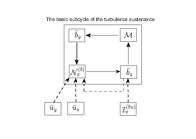
Figure 15: Sketch of the basic subcycle of the sustaining process (the solid arrows within the rectangle): (i) generation of $\bar{b}_{x}$ by the nonlinearity ${\cal N}_{x}^{(b)}$, (ii) subsequent production of ${\cal M}$ from $\bar{b}_{x}$ and (iii) of the azimuthal field energy $|\bar{b}_{y}|^{2}$ by ${\cal M}$ (the linear MRI stage) and finally (iv) the nonlinear feedback – contribution of $\bar{b}_{y}$ to ${\cal N}_{x}^{(b)}$. The other contributions (dashed arrows) of ${\cal I}_{x}^{(bu)}$ to the production of $\bar{b}_{x}$ and the feedback of $\bar{u}_{x},\bar{u}_{y},\bar{b}_{x}$ to ${\cal N}_{x}^{b}$ ($\bar{u}_{z}$ and $\bar{b}_{z}$ are small and not shown), are a part of the overall sustaining scheme, but outside the basic subcycle.

5.1 The basic subcycle of the turbulence sustenance

As we already mentioned, the sustenance of the turbulence is the result of a subtle intertwining of the anisotropic linear transient growth and nonlinear transverse cascade processes, which have been described in the previous section. The intertwined character of these processes is too complex for a vivid schematization. Nevertheless, based on the insight into the turbulence dynamics gained from Figures 9-14, we can bring out the basic subcycle of the sustenance that clearly shows the equal importance of the linear and nonlinear processes. The azimuthal and radial magnetic field components are most energy-containing in this case. The basic subcycle of the turbulence sustenance, which is concentrated in the vital area in Fourier space, is sketched in Figure (15) (solid arrows within a rectangle) and can be understood as follows. The nonlinear term ${\cal N}_{x}^{(b)}$ contributes to the generation of the radial field $\bar{b}_{x}$ through the transverse cascade process. In other words, ${\cal N}_{x}^{(b)}$ provides a positive feedback for the continual regeneration of the radial field, which, in turn, is a seed/trigger for the linear growth of the MRI – $\bar{b}_{x}$ creates and amplifies the Maxwell stress, ${\cal M}$, due to the shear (via linear term in Equation B6 proportional to $q$). The positive stress then increases the dominant azimuthal field energy $|\bar{b}_{y}|^{2}/2$ at the expense of the mean flow, opposing the negative nonlinear term ${\cal N}_{y}^{(b)}$ (and resistive dissipation). Thus, this central energy gain process for turbulence, as mentioned before, is of linear nature and a consequence of the azimuthal MRI. The linearly generated $\bar{b}_{y}$ gives a dominant contribution – positive feedback – to the nonlinear term ${\cal N}_{x}^{(b)}$, closing the basic subcycle.

This is only a main part of the complete and more intricate sustaining scheme that involves also the velocity components. In this sketch, the dashed arrows denote the other, extrinsic to the basic subcycle, processes. Namely, $\bar{b}_{x}$, together with the nonlinear term, is fueled also by the linear exchange term, ${\cal I}_{x}^{(bu)}$, which takes energy from the radial velocity $\bar{u}_{x}$, while the azimuthal velocity $\bar{u}_{y}$ gets energy from $\bar{b}_{y}$ via the linear exchange term ${\cal I}_{y}^{(ub)}$. These are all linear processes, part of the MRI. (The vertical velocity does not explicitly participate in this case.) All These components of the velocity $\bar{u}_{x}$, $\bar{u}_{y}$, $\bar{u}_{z}$ and the magnetic field $\bar{b}_{x}$, $\bar{b}_{z}$ then contribute to the nonlinear feedback through the nonlinear term for the radial field, ${\cal N}_{x}^{(b)}$, which is the most important one in the sustenance (see Equations B37), but still the contribution of $\bar{b}_{y}$ in this nonlinear term is dominant. This feedback process is essentially 3D: we verified that modes with $|k_{z}|=1,2$ give the largest contribution to the horizontal integral in the expression for the nonlinear term ${\cal N}_{x}^{(b)}$ (not shown here).

It is appropriate here to give a comparative analysis of the dynamical processes investigated in this paper and those underlying sustained 3D MRI-dynamo cycles reported in Herault et al. (2011) and Riols et al. (2015, 2017), despite the fact that these papers considered a magnetized Keplerian flow with different, zero net vertical flux, configuration and different values of parameters (smaller resolution, box aspect ratio, smaller Reynolds numbers) than those adopted here. These apparently resulted in the resistive processes penetrating into the vital area (in our terms) and reducing a number of active modes to only first non-axisymmetric ones (shearing waves) with the minimal azimuthal and vertical wavenumbers, $k_{y}=2\pi/L_{y},k_{z}=0,2\pi/L_{z}$, which undergo the transient MRI due to the mean axisymmetric azimuthal (dynamo) field. By contrast, the number of the active modes in our turbulent case is more than hundred (Figure 7). Regardless of these differences, we can trace the similarities in the sustenance cycles – the energy budget equations for these modes derived in those papers in fact show that a similar scheme underlies the sustenance as in the present case. The energy of the radial field $\bar{b}_{x}$ of new leading non-axisymmetric modes is supplied by the joint action of the induction term (i.e., ${\cal I}_{x}^{(bu)}$ in our notations) and redistribution by the nonlinear term, however, a summation over $k_{x}$ as used in those energy budget equations does not permit to see how this nonlinear redistribution of modes over $k_{x}$ due to the transverse cascade actually occurs in their analysis. As for the energy of $\bar{b}_{y}$, it is amplified by the Maxwell stress during the transient MRI phase (also called the $\Omega$-effect) and is drained by the corresponding nonlinear term. Since in the turbulent state considered here there are much more active modes, representing various linear and nonlinear dynamical terms in $(k_{x},k_{y})$-plane has a definite advantage over such low-mode-number models in that gives a more general picture of nonlinear triad interactions among all active modes. Such a comparison raises one more point for thought: for a correct consideration of nonlinear triad interactions, we gave preference to boxes symmetrical in $(x,y)$-plane, while, all simulations in those papers are carried out in azimuthally elongated boxes.

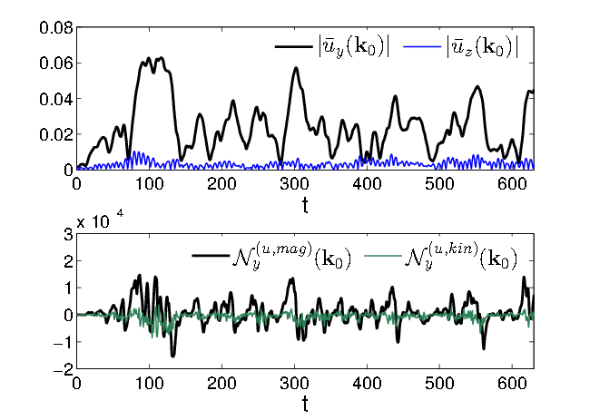
Figure 16: Evolution of the large-scale mode ${\bf k}_{0}=(1,0,0)$, which corresponds to the axisymmetric zonal flow. Shown are the amplitudes of the azimuthal $|\bar{u}_{y}|$ (black) and the vertical $|\bar{u}_{z}|$ (blue) velocities (upper panel) as well as the magnetic ${\cal N}_{y}^{(u,mag)}$ (black) and hydrodynamic ${\cal N}_{y}^{(u,kin)}$ (green) parts of the nonlinear term ${\cal N}_{y}^{(u)}$ (lower panel). The dominant azimuthal velocity (i.e., zonal flow) is driven by the magnetic part of the nonlinear term and is characterized by remarkably slower time variations.

5.2 Zonal flow

Excitation of zonal flows by the MRI-turbulence was previously observed by Johansen et al. (2009) and Bai & Stone (2014) in the case of zero and nonzero net vertical magnetic flux, respectively. We also observe it here in the case of the net azimuthal field. As noted above, the mode corresponding to the zonal flow is axisymmetric and vertically constant, $k_{y}=k_{z}=0$, with large scale variation in the radial direction, $|k_{x}|=1$. The divergence-free (incompressibility) condition (B8) implies that the radial velocity is zero, $\bar{u}_{x}=0$, for this mode and hence ${\cal H}_{y}=0$ at all times, also the magnetic exchange term is identically zero at $k_{y}=0$, ${\cal I}_{y}^{(ub)}=0$. Therefore, a source of the zonal flow can be only the nonlinear term ${\cal N}_{y}^{(u)}$ in Equation (12). We can divide this term into the magnetic, ${\cal N}^{(u,mag)}_{y}$, and hydrodynamic, ${\cal N}^{(u,kin)}_{y}$, parts,

$${\cal N}^{(u)}_{y}={\cal N}^{(u,mag)}_{y}+{\cal N}^{(u,kin)}_{y}.$$ (23)

For the dominant mode ${\bf k_{0}}=(1,0,0)$, these two parts in Equation (23) have the forms:

$${\cal N}^{(u,mag)}_{y}({\bf k}_{0},t)\\ =\frac{\rm i}{2}\bar{u}^{\ast}_{y}({\bf k}_{0},t)\int d^{3}{\bf k^{\prime}}\bar{b}_{y}({\bf k^{\prime}},t)\bar{b}_{x}({\bf k}_{0}-{\bf k^{\prime}},t)+c.c.,$$ (24)

with the integrand composed of the turbulent magnetic stresses and

$${\cal N}^{(u,kin)}_{y}({\bf k}_{0},t)\\ =-\frac{\rm i}{2}\bar{u}^{\ast}_{y}({\bf k}_{0},t)\int d^{3}{\bf k^{\prime}}\bar{u}_{y}({\bf k^{\prime}},t)\bar{u}_{x}({\bf k}_{0}-{\bf k^{\prime}},t)+c.c.,$$ (25)

with the integrand composed of the turbulent hydrodynamic stresses. To understand the nature of the zonal flow, in Figure 16 we present the time-development of the azimuthal and vertical velocities as well as the driving nonlinear terms for this mode. $|u_{y}({\bf k_{0}},t)|$ is characterized by remarkably longer timescale (tens of orbits) variations and prevails over rapidly oscillating $|u_{z}({\bf k_{0}},t)|$, i.e., the dominant harmonic indeed forms a slowly varying in time axisymmetric zonal flow. Comparing the time-development of $|\bar{u}_{y}({\bf k}_{0},t)|$ with that of the corresponding nonlinear terms in the lower panel of Figure 16, we clearly see that it is driven primarily by the magnetic nonlinear term, ${\cal N}^{(u,mag)}_{y}({\bf k_{0}},t)$, which physically describes the effect of the total azimuthal magnetic tension (random forcing) exerted by all other smaller-scale modes on the large-scale ${\bf k}_{0}$ mode, whereas ${\cal N}^{(u,kin)}_{y}({\bf k_{0}},t)$, corresponding to the net effect of the hydrodynamic stresses, is much smaller than the magnetic one. The important role of the magnetic perturbations in launching and maintaining the zonal flow is consistent with the findings of Johansen et al. (2009).

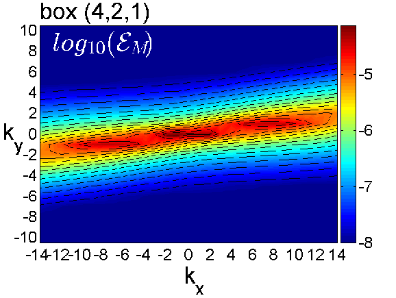
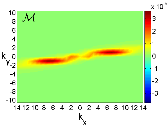
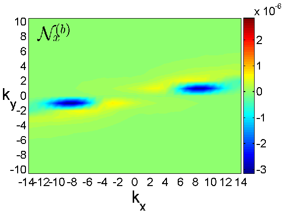
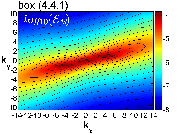
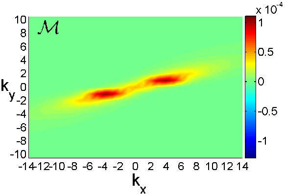
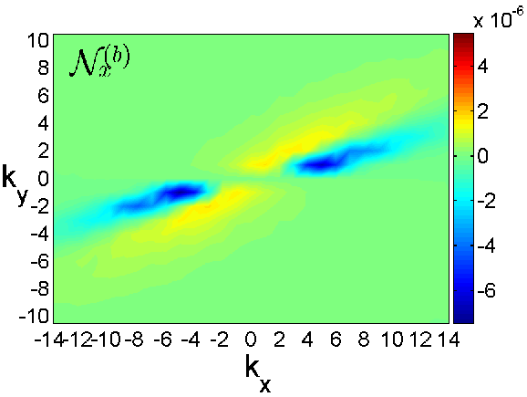
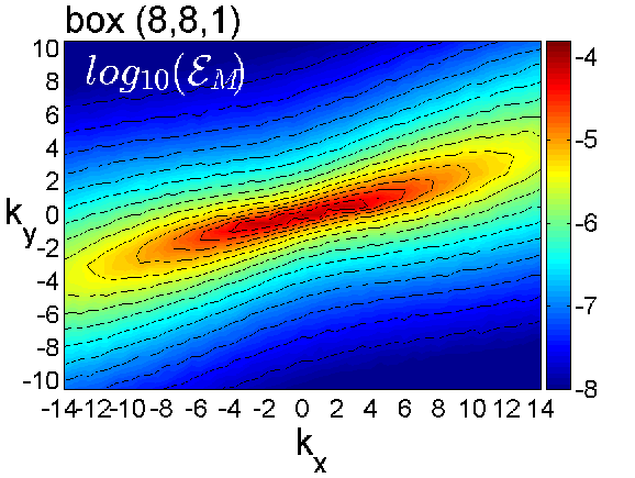
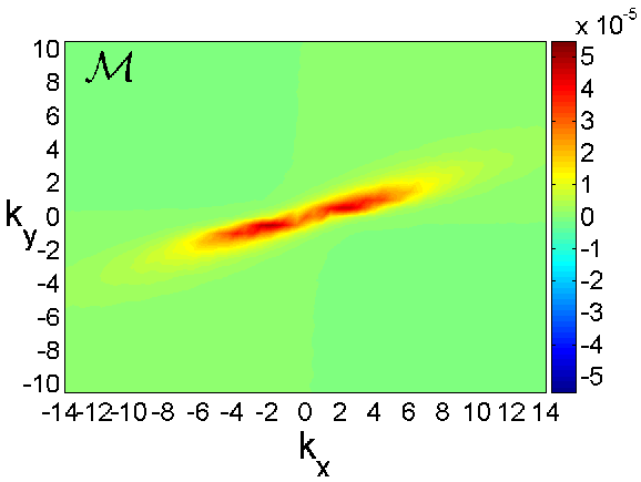
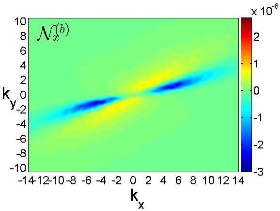
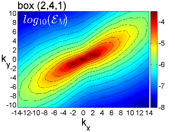
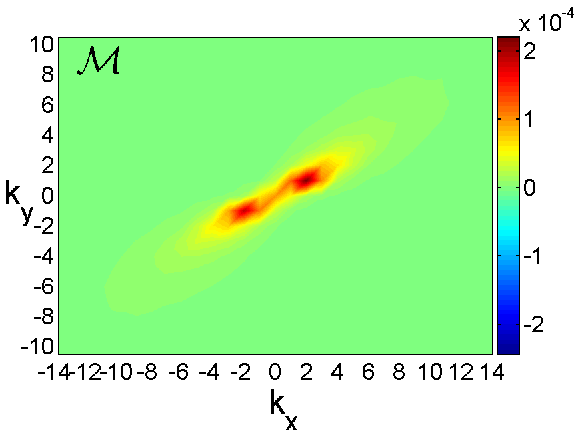
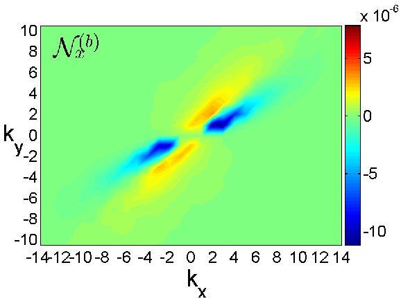
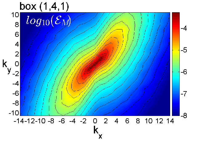
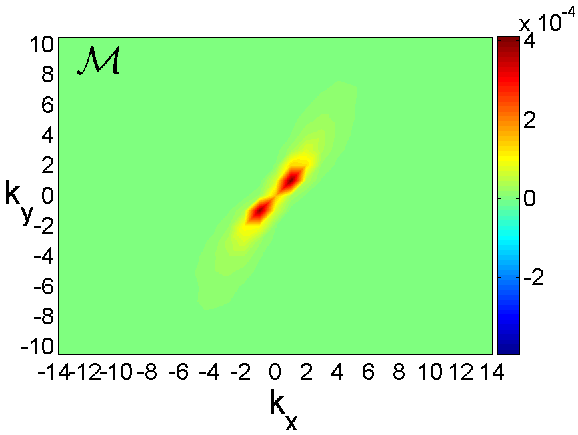
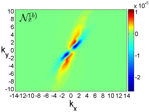
Figure 17: Spectra of ${\cal E}_{M}$, ${\cal M}$ and ${\cal N}^{(b)}_{x}$ in $(k_{x},k_{y})$-plane at $k_{z}=1$ for all the boxes: $(4,2,1)$ (top row), $(4,4,1)$ (second row), $(8,8,1)$ (third row), $(2,4,1)$ (fourth row) and $(1,4,1)$ (bottom row). In all the panels, the general structure of these spectral terms is quite similar, that indicates the universality and the robust character of the turbulence sustaining scheme. At the same time, the symmetric boxes $(4,4,1)$ and $(8,8,1)$ have similar spectral pictures with identical inclinations, while in the asymmetric in $(x,y)$-plane boxes, the spectral characteristics are somewhat deformed and have different inclinations compared to the symmetric boxes.

5.3 Effect of the aspect ratio and the universality of the turbulence sustenance scheme

The main advantage of the box $(4,4,1)$ analyzed in the previous subsection is that (i) it is symmetric in physical $(x,y)$-and Fourier $(k_{x},k_{y})$-planes, where the effects of shear are most important, (ii) the modes contained in this box densely cover the vital area in $(k_{x},k_{y})$-plane and sufficiently comprise effectively growing (optimal) harmonics (see the panel for the box $(4,4,1)$ in Figure 2). In the three asymmetric boxes – $(1,4,1)$, $(2,4,1)$ and $(4,2,1)$ – the modes less densely cover the vital area (Figure 2). As for the box $(8,8,1)$, as mentioned above, the results qualitatively similar to the box $(4,4,1)$ are expected. In this subsection, we examine how the box aspect ratio influences the turbulence dynamics, and in particular, the distribution of the linear and nonlinear process in Fourier space.

A general temporal behavior of the volume-averaged energies, stresses and rms values of the velocity and magnetic field components is similar to that for the box $(4,4,1)$ represented in Figure 3 (see also Table 1) and we do not show it here, but concentrate instead on the differences in Fourier space. Figure 17 juxtaposes the spectra of the magnetic energy, Maxwell stress and the magnetic nonlinear term ${\cal N}_{x}^{(b)}$ for all the boxes. From this figure it is evident that the skeleton of the balances of the various linear and nonlinear processes and, in particular the basic subcycle, underlying the sustenance of the azimuthal MRI-turbulence are qualitatively the same in all the simulated boxes and quite robust – the variations in box sizes do not affect its effectiveness. Changes in box aspect ratios lead to variation of the inclinations, shapes and intensities of the energy spectra as well as the distribution of linear and nonlinear dynamical terms in $(k_{x},k_{y})$-plane. It is seen in Figure 17 that this variation is minimal between the symmetric in $(x,y)$-plane boxes $(4,4,1)$ and $(8,8,1)$ – they have similar spectral characteristics with identical inclination angles – but is more remarkable among the asymmetric boxes, $(4,2,1)$, $(2,4,1)$, $(1,4,1)$. Specifically, in the latter boxes, the spectral characteristics are somewhat deformed and have different inclinations compared to those in the symmetric boxes. The reason for this is the reduction of the active modes’ number/density along the $k_{x}$- and $k_{y}$-axis in these boxes in contrast to the symmetric ones (see Figure 2).

6 Summary and discussion

In this paper, we elucidated the essence of the sustenance of MRI-driven turbulence in Keplerian disks threaded by a nonzero net azimuthal field by means of a series of shearing box simulations and analysis in 3D Fourier (k-)space. It is well known that in the linear regime the MRI in the presence of a azimuthal field has a transient nature and eventually decays without an appropriate nonlinear feedback. We studied in detail the linear and nonlinear dynamical processes and their interplay in Fourier space that ensure such a feedback. Our first key finding is the pronounced anisotropy of the nonlinear processes in k-space. This anisotropy is a natural consequence of the anisotropy of linear processes due to the shear and cannot be described in the framework of direct and inverse cascades, commonly considered in the classical theory of HD and MHD turbulence without shear, because the main activity of the nonlinear processes is transfer of modes over wavevector orientation (angle) in k-space, rather than along wavevector that corresponds to direct/inverse cascades. This new type of nonlinear process – the transverse cascade – plays a decisive role in the long-term maintenance of the MRI-turbulence. Our second key result is that the sustenance of the turbulence in this case is ensured as a result of a subtle interplay of the linear transient MRI growth and nonlinear transverse cascade. This interplay is intrinsically quite complex. Nevertheless, one can isolate the basic subcycle of the turbulence sustenance, which is as follows. The linear exchange of energy between the magnetic field and the background flow, realized by the Maxwell stress, ${\cal M}$, supplies only the azimuthal field component $\bar{b}_{y}$. As for the radial field $\bar{b}_{x}$, it is powered by the linear exchange ${\cal I}_{x}^{(bu)}$ and the nonlinear ${\cal N}^{(b)}_{x}$ terms. So, $\bar{b}_{x}$ and $\bar{b}_{y}$ have sources of different origin. However, one should bear in mind that these processes are intertwined with each other: the source of $\bar{b}_{y}$ (i.e., the Maxwell stress, ${\cal M}$) is created by $\bar{b}_{x}$. In its turn, the production of the nonlinear source of $\bar{b}_{x}$ (i.e., ${\cal N}^{(b)}_{x}$) is largely due to $\bar{b}_{y}$. Similarly intertwined are the dynamics of other spectral magnetic and kinematic components. This sustaining dynamics of the turbulence is concentrated mainly in a small wavenumber area of k-space, i.e., involves large scale modes, and is appropriately called the vital area.

The spectra of the kinetic and magnetic energies that are established in the turbulent state as a result of such interplay are consequently also anisotropic and fundamentally differ from classical Kolmogorov or IK spectra. So, the conventional characterization of nonlinear MHD cascade processes in shear flows in terms of direct and inverse cascades, which ignores the shear-induced spectral anisotropy and the resulting important transverse cascade process, is generally incomplete and misleading. For this reason, we examined the dynamical processes in 3D Fourier space in full without making the shell-averaging, which has been commonly done in previous studies of MRI-turbulence and smears out the anisotropy. We also showed that the turbulence is accompanied by a large scale and slowly varying in time zonal (azimuthal) flow, which is driven by the turbulent magnetic stresses.

The proposed scheme of the turbulence sustenance based on the intertwined cooperated action of the linear and nonlinear processes in the vital area is quite robust – it is effective for different aspect ratios of the simulation box. For all the box configurations considered, $(4,4,1)$, $(1,4,1)$, $(2,4,1)$, $(4,2,1)$ and $(8,8,1)$, the scheme is essentially universal, although there are quantitative differences. The anisotropy of the box in $(k_{x},k_{y})$-plane is superposed on the intrinsic shear-induced anisotropy of the dynamical process and somewhat deforms the picture of the turbulence, but the sustaining scheme is not changed. In any case, an isotropic distribution of modes in $(k_{x},k_{y})$-plane seems preferable for studying the own anisotropy of the shear flow system, which is naturally achieved for equal radial and azimuthal sizes, $L_{x}=L_{y}$, of the box.

In this paper, we considered a spectrally stable (i.e., without purely exponential MRI) magnetized disk flow with an azimuthal field, where the energy for turbulence can only be supplied via linear transient growth of the MRI. Being associated with shear, it seems obvious that the vital area and nonlinear transverse cascade should be also present in disk flows with a nonzero net vertical magnetic field, which can give rise to the exponentially growing MRI (Balbus & Hawley, 1991; Goodman & Xu, 1994; Pessah & Goodman, 2009). In this case, besides purely exponentially growing axisymmetric (channel) modes, energy supply and transport via (transient) growth of non-axisymmetric ($k_{y}\neq 0$) modes are also important (Longaretti & Lesur, 2010; Mamatsashvili et al., 2013; Squire & Bhattacharjee, 2014). The latter, leading to anisotropic nonlinear dynamics (Murphy & Pessah, 2015), can inevitably effect the nonlinear transverse cascade process. However, the presence of the purely exponentially growing modes should somewhat alter the scheme of the interplay of the dynamical processes that we studied here in the case of the azimuthal field. We plan to explore this interplay also in the case of vertical field MRI-turbulence, which will be published elsewhere.

An interesting application of this approach – analysis of turbulence dynamics in Fourier space – and a natural extension of the present study would be understanding the nature of MRI turbulence with zero net magnetic flux, where the classical linear exponentially growing MRI is absent. This case has been studied in several different configurations and there is much debate over the nature of dynamo action, whether it is small-scale or large-scale (Lesur & Ogilvie, 2008; Davis et al., 2010; Gressel, 2010; Bodo et al., 2011, 2012, 2013; Hirose et al., 2014; Shi et al., 2016), and on the convergence with increasing resolution/Reynolds number (Pessah et al., 2007; Fromang & Papaloizou, 2007; Fromang, 2010; Bodo et al., 2011, 2014). A study of this kind will therefore be very helpful in the resolution of these issues. In this regard, we would like to mention recent high-resolution and high-Reynolds number simulations of MRI-turbulence by Walker et al. (2016) and Zhdankin et al. (2017), resolving larger wavenumbers outside the vital area – inertial and dissipation ranges. It was shown that the properties of turbulence at these wavenumbers are insensitive to the specific nature of the imposed large-scale magnetic field and are similar to those of classical MHD turbulence without shear. In particular, the characteristic energy spectra of the inertial range is close to the IK spectrum, provided the energy of the large-scale azimuthal magnetic field fluctuations is subtracted, while the small-scale viscous and resistive dissipation characteristics are almost unaffected by the presence of MRI. These studies, focusing on larger wavenumbers, combined with our analysis, which focuses instead on smaller wavenumbers that carry most of the energy and stress, should be fruitful in shedding light on the dynamical picture of zero-net flux MRI-turbulence.

Appendix A Perturbation equations in physical space

Equations governing the evolution of the velocity, total pressure and magnetic field perturbations, ${\bf u},p,{\bf b}$, about the equilibrium Keplerian flow ${\bf U}_{0}=(0,-q\Omega x,0)$ with net azimuthal field ${\bf B}_{0}=(0,B_{0y},0)$ are obtained from the basic Equations (1)-(5) and componentwise have the form:

$$\frac{Du_{x}}{Dt}=2\Omega u_{y}-\frac{1}{\rho_{0}}\frac{\partial p}{\partial x}+\frac{B_{0y}}{4\pi\rho_{0}}\frac{\partial b_{x}}{\partial y}+\frac{\partial}{\partial x}\left(\frac{b_{x}^{2}}{4\pi\rho_{0}}-u_{x}^{2}\right)+\frac{\partial}{\partial y}\left(\frac{b_{x}b_{y}}{4\pi\rho_{0}}-u_{x}u_{y}\right)+\frac{\partial}{\partial z}\left(\frac{b_{x}b_{z}}{4\pi\rho_{0}}-u_{x}u_{z}\right)+\nu\nabla^{2}u_{x},$$ (A1)

$$\frac{Du_{y}}{Dt}=(q-2)\Omega u_{x}-\frac{1}{\rho_{0}}\frac{\partial p}{\partial y}+\frac{B_{0y}}{4\pi\rho_{0}}\frac{\partial b_{y}}{\partial y}+\\ +\frac{\partial}{\partial x}\left(\frac{b_{x}b_{y}}{4\pi\rho_{0}}-u_{x}u_{y}\right)+\frac{\partial}{\partial y}\left(\frac{b_{y}^{2}}{4\pi\rho_{0}}-u_{y}^{2}\right)+\frac{\partial}{\partial z}\left(\frac{b_{z}b_{y}}{4\pi\rho_{0}}-u_{z}u_{y}\right)+\nu\nabla^{2}u_{y}$$ (A2)

$$\frac{Du_{z}}{Dt}=-\frac{1}{\rho_{0}}\frac{\partial p}{\partial z}-N^{2}\theta+\frac{B_{0y}}{4\pi\rho_{0}}\frac{\partial b_{z}}{\partial y}+\\ +\frac{\partial}{\partial x}\left(\frac{b_{x}b_{z}}{4\pi\rho_{0}}-u_{x}u_{z}\right)+\frac{\partial}{\partial y}\left(\frac{b_{y}b_{z}}{4\pi\rho_{0}}-u_{y}u_{z}\right)+\frac{\partial}{\partial z}\left(\frac{b_{z}^{2}}{4\pi\rho_{0}}-u_{z}^{2}\right)+\nu\nabla^{2}u_{z}$$ (A3)

$$\frac{D\theta}{Dt}=u_{z}-\frac{\partial}{\partial x}(u_{x}\theta)-\frac{\partial}{\partial y}(u_{y}\theta)-\frac{\partial}{\partial z}(u_{z}\theta)+\chi\nabla^{2}\theta$$ (A4)

$$\frac{Db_{x}}{Dt}=B_{0y}\frac{\partial u_{x}}{\partial y}+\frac{\partial}{\partial y}\left(u_{x}b_{y}-u_{y}b_{x}\right)-\frac{\partial}{\partial z}(u_{z}b_{x}-u_{x}b_{z})+\eta\nabla^{2}b_{x},$$ (A5)

$$\frac{Db_{y}}{Dt}=-q\Omega b_{x}+B_{0y}\frac{\partial u_{y}}{\partial y}-\frac{\partial}{\partial x}\left(u_{x}b_{y}-u_{y}b_{x}\right)+\frac{\partial}{\partial z}(u_{y}b_{z}-u_{z}b_{y})+\eta\nabla^{2}b_{y},$$ (A6)

$$\frac{Db_{z}}{Dt}=B_{0y}\frac{\partial u_{z}}{\partial y}+\frac{\partial}{\partial x}\left(u_{z}b_{x}-u_{x}b_{z}\right)-\frac{\partial}{\partial y}(u_{y}b_{z}-u_{z}b_{y})+\eta\nabla^{2}b_{z},$$ (A7)

$$\frac{\partial u_{x}}{\partial x}+\frac{\partial u_{y}}{\partial y}+\frac{\partial u_{z}}{\partial z}=0,$$ (A8)

$$\frac{\partial b_{x}}{\partial x}+\frac{\partial b_{y}}{\partial y}+\frac{\partial b_{z}}{\partial z}=0,$$ (A9)

where $D/Dt=\partial/\partial t-q\Omega x\partial/\partial y$ is the total derivative along the background flow.

Appendix B Derivation of spectral equations for quadratic terms

Here we derive evolution equations for velocity, entropy and magnetic field perturbations in Fourier space. Substituting decomposition (10) into Equations (A1)-(A9) and taking into account the normalization made in the text, we arrive at the following equations governing the dynamics of perturbation modes in Fourier space

$$\left(\frac{\partial}{\partial t}+qk_{y}\frac{\partial}{\partial k_{x}}\right)\bar{u}_{x}=2\bar{u}_{y}-{\rm i}k_{x}\bar{p}+{\rm i}k_{y}B_{0y}\bar{b}_{x}-\frac{k^{2}}{\rm Re}\bar{u}_{x}+{\rm i}k_{x}N^{(u)}_{xx}+{\rm i}k_{y}N^{(u)}_{xy}+{\rm i}k_{z}N^{(u)}_{xz},$$ (B1)

$$\left(\frac{\partial}{\partial t}+qk_{y}\frac{\partial}{\partial k_{x}}\right)\bar{u}_{y}=(q-2)\bar{u}_{x}-{\rm i}k_{y}\bar{p}+{\rm i}k_{y}B_{0y}\bar{b}_{y}-\frac{k^{2}}{\rm Re}\bar{u}_{y}+{\rm i}k_{x}N^{(u)}_{xy}+{\rm i}k_{y}N^{(u)}_{yy}+{\rm i}k_{z}N^{(u)}_{yz},$$ (B2)

$$\left(\frac{\partial}{\partial t}+qk_{y}\frac{\partial}{\partial k_{x}}\right)\bar{u}_{z}=-{\rm i}k_{z}\bar{p}-N^{2}\bar{\theta}+{\rm i}k_{y}B_{0y}\bar{b}_{z}-\frac{k^{2}}{\rm Re}\bar{u}_{z}+{\rm i}k_{x}N^{(u)}_{xz}+{\rm i}k_{y}N^{(u)}_{yz}+{\rm i}k_{z}N^{(u)}_{zz},$$ (B3)

$$\left(\frac{\partial}{\partial t}+qk_{y}\frac{\partial}{\partial k_{x}}\right)\bar{\theta}=\bar{u}_{z}-\frac{k^{2}}{\rm Pe}\bar{\theta}+{\rm i}k_{x}N^{(\theta)}_{x}+{\rm i}k_{y}N^{(\theta)}_{y}+{\rm i}k_{z}N^{(\theta)}_{z},$$ (B4)

$$\left(\frac{\partial}{\partial t}+qk_{y}\frac{\partial}{\partial k_{x}}\right)\bar{b}_{x}={\rm i}k_{y}B_{0y}\bar{u}_{x}-\frac{k^{2}}{\rm Rm}\bar{b}_{x}+{\rm i}k_{y}\bar{F}_{z}-{\rm i}k_{z}\bar{F}_{y},$$ (B5)

$$\left(\frac{\partial}{\partial t}+qk_{y}\frac{\partial}{\partial k_{x}}\right)\bar{b}_{y}=-q\bar{b}_{x}+{\rm i}k_{y}B_{0y}\bar{u}_{y}-\frac{k^{2}}{\rm Rm}\bar{b}_{y}+{\rm i}k_{z}\bar{F}_{x}-{\rm i}k_{x}\bar{F}_{z}$$ (B6)

$$\left(\frac{\partial}{\partial t}+qk_{y}\frac{\partial}{\partial k_{x}}\right)\bar{b}_{z}={\rm i}k_{y}B_{0y}\bar{u}_{z}-\frac{k^{2}}{\rm Rm}\bar{b}_{z}+{\rm i}k_{x}\bar{F}_{y}-{\rm i}k_{y}\bar{F}_{x}$$ (B7)

$$k_{x}\bar{u}_{x}+k_{y}\bar{u}_{y}+k_{z}\bar{u}_{z}=0,$$ (B8)

$$k_{x}\bar{b}_{x}+k_{y}\bar{b}_{y}+k_{z}\bar{b}_{z}=0,$$ (B9)

where $k^{2}=k_{x}^{2}+k_{y}^{2}+k_{z}^{2}$ and $B_{0y}=\sqrt{2/\beta}$ is the normalized background azimuthal field. These spectral equations contain the linear as well as the nonlinear ($N^{(u)}_{ij}({\bf k},t),N^{(\theta)}_{i}({\bf k},t),\bar{F}_{i}({\bf k},t)$, $i,j=x,y,z$) terms that are the Fourier transforms of the corresponding linear and nonlinear terms in the original Equations (A1)-(A9). The latter are given by convolutions

$$N^{(u)}_{ij}({\bf k},t)=\int d^{3}{\bf k^{\prime}}\left[\bar{b}_{i}({\bf k^{\prime}},t)\bar{b}_{j}({\bf k}-{\bf k^{\prime}},t)-\bar{u}_{i}({\bf k^{\prime}},t)\bar{u}_{j}({\bf k}-{\bf k^{\prime}},t)\right],$$ (B10)

$$N^{(\theta)}_{i}({\bf k},t)=-\int d^{3}{\bf k^{\prime}}\bar{u}_{i}({\bf k^{\prime}},t)\bar{\theta}({\bf k}-{\bf k^{\prime}},t)$$ (B11)

where $i,j=x,y,z$ and $\bar{F}_{x},\bar{F}_{y},\bar{F}_{z}$ are the fourier transforms of the respective components of the perturbed electromotive force ${\bf F}={\bf u}\times{\bf b}$,

$$\bar{F}_{x}({\bf k},t)=\int d^{3}{\bf k^{\prime}}\left[\bar{u}_{y}({\bf k^{\prime}},t)\bar{b}_{z}({\bf k}-{\bf k^{\prime}},t)-\bar{u}_{z}({\bf k^{\prime}},t)\bar{b}_{y}({\bf k}-{\bf k^{\prime}},t)\right]$$

$$\bar{F}_{y}({\bf k},t)=\int d^{3}{\bf k^{\prime}}\left[\bar{u}_{z}({\bf k^{\prime}},t)\bar{b}_{x}({\bf k}-{\bf k^{\prime}},t)-\bar{u}_{x}({\bf k^{\prime}},t)\bar{b}_{z}({\bf k}-{\bf k^{\prime}},t)\right]$$

$$\bar{F}_{z}({\bf k},t)=\int d^{3}{\bf k^{\prime}}\left[\bar{u}_{x}({\bf k^{\prime}},t)\bar{b}_{y}({\bf k}-{\bf k^{\prime}},t)-\bar{u}_{y}({\bf k^{\prime}},t)\bar{b}_{x}({\bf k}-{\bf k^{\prime}},t)\right]$$

and describe the contribution from nonlinearity to the magnetic field perturbations. In the case of classical forced MHD turbulence without background shear flow, these nonlinear transfer terms in ${\bf k}$-space were also derived in Verma (2004). From Equations (B1)-(B3) and the divergence-free conditions (B8) and (B9) we can eliminate pressure

$$\bar{p}=2{\rm i}(1-q)\frac{k_{y}}{k^{2}}\bar{u}_{x}-2{\rm i}\frac{k_{x}}{k^{2}}\bar{u}_{y}+{\rm i}N^{2}\frac{k_{z}}{k^{2}}\bar{\theta}+\sum_{(i,j)=(x,y,z)}\frac{k_{i}k_{j}}{k^{2}}N^{(u)}_{ij}$$ (B12)

Substituting it back into Equations (B1)-(B3) we get

$$\left(\frac{\partial}{\partial t}+qk_{y}\frac{\partial}{\partial k_{x}}\right)\bar{u}_{x}=2\left(1-\frac{k_{x}^{2}}{k^{2}}\right)\bar{u}_{y}+2(1-q)\frac{k_{x}k_{y}}{k^{2}}\bar{u}_{x}+N^{2}\frac{k_{x}k_{z}}{k^{2}}\bar{\theta}+{\rm i}k_{y}B_{0y}\bar{b}_{x}-\frac{k^{2}}{\rm Re}\bar{u}_{x}+Q_{x},$$ (B13)

$$\left(\frac{\partial}{\partial t}+qk_{y}\frac{\partial}{\partial k_{x}}\right)\bar{u}_{y}=\left[q-2-2(q-1)\frac{k_{y}^{2}}{k^{2}}\right]\bar{u}_{x}-2\frac{k_{x}k_{y}}{k^{2}}\bar{u}_{y}+N^{2}\frac{k_{y}k_{z}}{k^{2}}\bar{\theta}+{\rm i}k_{y}B_{0y}\bar{b}_{y}-\frac{k^{2}}{\rm Re}\bar{u}_{y}+Q_{y},$$ (B14)

$$\left(\frac{\partial}{\partial t}+qk_{y}\frac{\partial}{\partial k_{x}}\right)\bar{u}_{z}=2(1-q)\frac{k_{y}k_{z}}{k^{2}}\bar{u}_{x}-2\frac{k_{x}k_{z}}{k^{2}}\bar{u}_{y}-N^{2}\left(1-\frac{k_{z}^{2}}{k^{2}}\right)\bar{\theta}+{\rm i}k_{y}B_{0y}\bar{b}_{z}-\frac{k^{2}}{\rm Re}\bar{u}_{z}+Q_{z},$$ (B15)

where

$$Q_{i}={\rm i}\sum_{j}k_{j}N^{(u)}_{ij}-{\rm i}k_{i}\sum_{m,n}\frac{k_{m}k_{n}}{k^{2}}N^{(u)}_{mn},~{}~{}~{}~{}~{}i,j,m,n=x,y,z.$$ (B16)

Multiplying Equations (B13)-(B15), respectively, by $\bar{u}_{x}^{\ast}$, $\bar{u}_{y}^{\ast}$, $\bar{u}_{z}^{\ast}$, and adding up with their complex conjugates, we obtain

$$\frac{\partial}{\partial t}\frac{|\bar{u}_{x}|^{2}}{2}=-qk_{y}\frac{\partial}{\partial k_{x}}\frac{|\bar{u}_{x}|^{2}}{2}+{\cal H}_{x}+{\cal I}_{x}^{(u\theta)}+{\cal I}_{x}^{(ub)}+{\cal D}_{x}^{(u)}+{\cal N}^{(u)}_{x},$$ (B17)

$$\frac{\partial}{\partial t}\frac{|\bar{u}_{y}|^{2}}{2}=-qk_{y}\frac{\partial}{\partial k_{x}}\frac{|\bar{u}_{y}|^{2}}{2}+{\cal H}_{y}+{\cal I}_{y}^{(u\theta)}+{\cal I}_{y}^{(ub)}+{\cal D}_{y}^{(u)}+{\cal N}^{(u)}_{y},$$ (B18)

$$\frac{\partial}{\partial t}\frac{|\bar{u}_{z}|^{2}}{2}=-qk_{y}\frac{\partial}{\partial k_{x}}\frac{|\bar{u}_{z}|^{2}}{2}+{\cal H}_{z}+{\cal I}_{z}^{(u\theta)}+{\cal I}_{z}^{(ub)}+{\cal D}_{z}^{(u)}+{\cal N}^{(u)}_{z},$$ (B19)

where the terms of linear origin are

$${\cal H}_{x}=\left(1-\frac{k_{x}^{2}}{k^{2}}\right)(\bar{u}_{x}\bar{u}_{y}^{\ast}+\bar{u}_{x}^{\ast}\bar{u}_{y})+2(1-q)\frac{k_{x}k_{y}}{k^{2}}|\bar{u}_{x}|^{2},$$ (B20)

$${\cal H}_{y}=\frac{1}{2}\left[q-2-2(q-1)\frac{k_{y}^{2}}{k^{2}}\right](\bar{u}_{x}\bar{u}_{y}^{\ast}+\bar{u}_{x}^{\ast}\bar{u}_{y})-2\frac{k_{x}k_{y}}{k^{2}}|\bar{u}_{y}|^{2}$$ (B21)

$${\cal H}_{z}=(1-q)\frac{k_{y}k_{z}}{k^{2}}(\bar{u}_{x}\bar{u}_{z}^{\ast}+\bar{u}_{x}^{\ast}\bar{u}_{z})-\frac{k_{x}k_{z}}{k^{2}}(\bar{u}_{y}\bar{u}_{z}^{\ast}+\bar{u}_{y}^{\ast}\bar{u}_{z}),$$ (B22)

$${\cal I}_{i}^{(u\theta)}=N^{2}\left(\frac{k_{i}k_{z}}{k^{2}}-\delta_{iz}\right)\frac{\bar{\theta}\bar{u}_{i}^{\ast}+\bar{\theta}^{\ast}\bar{u}_{i}}{2},$$ (B23)

$${\cal I}_{i}^{(ub)}=\frac{\rm i}{2}k_{y}B_{0y}(\bar{u}_{i}^{\ast}\bar{b}_{i}-\bar{u}_{i}\bar{b}_{i}^{\ast}),$$ (B24)

$${\cal D}_{i}^{(u)}=-\frac{k^{2}}{\rm Re}|\bar{u}_{i}|^{2},$$ (B25)

and the modified nonlinear transfer functions for the quadratic forms of the velocity components are

$${\cal N}^{(u)}_{i}=\frac{1}{2}(\bar{u}_{i}Q^{\ast}_{i}+\bar{u}_{i}^{\ast}Q_{i}).$$ (B26)

Here $i=x,y,z$ and $\delta_{iz}$ is the Kronecker delta. It is readily shown that the sum of ${\cal H}_{i}$ is equal to the Reynolds stress spectrum multiplied by the shear parameter $q$, ${\cal H}={\cal H}_{x}+{\cal H}_{y}+{\cal H}_{z}=q(\bar{u}_{x}\bar{u}_{y}^{\ast}+\bar{u}_{x}^{\ast}\bar{u}_{y})/2$

Similarly, multiplying Equation (B4) by $\bar{\theta}^{\ast}$ and adding up with its complex conjugate, we get

$$\frac{\partial}{\partial t}\frac{|\bar{\theta}|^{2}}{2}=-qk_{y}\frac{\partial}{\partial k_{x}}\frac{|\bar{\theta}|^{2}}{2}+{\cal I}^{(\theta u)}+{\cal D}^{(\theta)}+{\cal N}^{(\theta)},$$ (B27)

where the terms of linear origin are

$${\cal I}^{(\theta u)}=\frac{1}{2}(\bar{u}_{z}\bar{\theta}^{\ast}+\bar{u}_{z}^{\ast}\bar{\theta}),$$ (B28)

$${\cal D}^{(\theta)}=-\frac{k^{2}}{\rm Pe}|\bar{\theta}|^{2}$$ (B29)

and the modified nonlinear transfer function for the quadratic form of the entropy is

$${\cal N}^{(\theta)}=\frac{\rm i}{2}\bar{\theta}^{\ast}(k_{x}N^{(\theta)}_{x}+k_{y}N^{(\theta)}_{y}+k_{z}N^{(\theta)}_{z})+c.c.$$ (B30)

Multiplying Equations (B5)-(B7), respectively, by $\bar{b}_{x}^{\ast}$, $\bar{b}_{y}^{\ast}$, $\bar{b}_{z}^{\ast}$, and adding up with their complex conjugates, we obtain

$$\frac{\partial}{\partial t}\frac{|\bar{b}_{x}|^{2}}{2}=-qk_{y}\frac{\partial}{\partial k_{x}}\frac{|\bar{b}_{x}|^{2}}{2}+{\cal I}_{x}^{(bu)}+{\cal D}_{x}^{(b)}+{\cal N}^{(b)}_{x}$$ (B31)

$$\frac{\partial}{\partial t}\frac{|\bar{b}_{y}|^{2}}{2}=-qk_{y}\frac{\partial}{\partial k_{x}}\frac{|\bar{b}_{y}|^{2}}{2}+{\cal M}+{\cal I}_{y}^{(bu)}+{\cal D}_{y}^{(b)}+{\cal N}^{(b)}_{y}$$ (B32)

$$\frac{\partial}{\partial t}\frac{|\bar{b}_{z}|^{2}}{2}=-qk_{y}\frac{\partial}{\partial k_{x}}\frac{|\bar{b}_{z}|^{2}}{2}+{\cal I}_{z}^{(bu)}+{\cal D}_{z}^{(b)}+{\cal N}^{(b)}_{z},$$ (B33)

where ${\cal M}$ is the Maxwell stress spectrum multiplied by $q$,

$${\cal M}=-\frac{q}{2}(\bar{b}_{x}\bar{b}_{y}^{\ast}+\bar{b}_{x}^{\ast}\bar{b}_{y}),$$ (B34)

$${\cal I}_{i}^{(bu)}=-{\cal I}_{i}^{(ub)}=\frac{\rm i}{2}k_{y}B_{0y}(\bar{u}_{i}\bar{b}_{i}^{\ast}-\bar{u}_{i}^{\ast}\bar{b}_{i})$$ (B35)

$${\cal D}_{i}^{(b)}=-\frac{k^{2}}{\rm Rm}|\bar{b}_{i}|^{2}$$ (B36)

and the modified nonlinear terms for the quadratic forms of the magnetic field components are

$${\cal N}^{(b)}_{x}=\frac{\rm i}{2}\bar{b}_{x}^{\ast}[k_{y}\bar{F}_{z}-k_{z}\bar{F}_{y}]+c.c.,~{}~{}~{}{\cal N}^{(b)}_{y}=\frac{\rm i}{2}\bar{b}_{y}^{\ast}[k_{z}\bar{F}_{x}-k_{x}\bar{F}_{z}]+c.c.,~{}~{}~{}{\cal N}^{(b)}_{z}=\frac{\rm i}{2}\bar{b}_{z}^{\ast}[k_{x}\bar{F}_{y}-k_{y}\bar{F}_{x}]+c.c.$$ (B37)

References

- Alexakis et al. (2007) Alexakis, A., Mininni, P. D., & Pouquet, A. 2007, New J. Phys., 9, 298
- Armitage (2011) Armitage, P. J. 2011, ARA&A, 49, 195
- Baggett et al. (1995) Baggett, J. S., Driscoll, T. A., & Trefethen, L. N. 1995, Phys. Fluids, 7, 833
- Bai & Stone (2014) Bai, X.-N., & Stone, J. M. 2014, ApJ, 796, 31
- Balbus (2003) Balbus, S. A. 2003, ARA & A, 41, 555
- Balbus & Hawley (1991) Balbus, S. A., & Hawley, J. F. 1991, ApJ, 376, 214
- Balbus & Hawley (1992) —. 1992, ApJ, 400, 610
- Beckwith et al. (2011) Beckwith, K., Armitage, P. J., & Simon, J. B. 2011, MNRAS, 416, 361
- Biskamp (2003) Biskamp, D. 2003, Magnetohydrodynamic turbulence (Cambridge University Press)
- Bodo et al. (2011) Bodo, G., Cattaneo, F., Ferrari, A., Mignone, A., & Rossi, P. 2011, ApJ, 739, 82
- Bodo et al. (2012) Bodo, G., Cattaneo, F., Mignone, A., & Rossi, P. 2012, ApJ, 761, 116
- Bodo et al. (2013) —. 2013, ApJ, 771, L23
- Bodo et al. (2014) —. 2014, ApJ, 787, L13
- Bodo et al. (2008) Bodo, G., Mignone, A., Cattaneo, F., Rossi, P., & Ferrari, A. 2008, A&A, 487, 1
- Brandenburg & Dintrans (2006) Brandenburg, A., & Dintrans, B. 2006, A&A, 450, 437
- Canuto et al. (1988) Canuto, C., Hussaini, M. Y., Quarteroni, A., & Zang, T. A. 1988, Spectral Methods in Fluid Dynamics (Springer)
- Chagelishvili et al. (2003) Chagelishvili, G. D., Zahn, J.-P., Tevzadze, A. G., & Lominadze, J. G. 2003, A&A, 402, 401
- Chapman (2002) Chapman, S. J. 2002, J. Fluid Mech., 451, 35
- Davis et al. (2010) Davis, S. W., Stone, J. M., & Pessah, M. E. 2010, ApJ, 713, 52
- Farrell & Ioannou (1996) Farrell, B. F., & Ioannou, P. J. 1996, Journal of Atmospheric Sciences, 53, 2025
- Fleming et al. (2000) Fleming, T. P., Stone, J. M., & Hawley, J. F. 2000, ApJ, 530, 464
- Flock et al. (2012a) Flock, M., Dzyurkevich, N., Klahr, H., Turner, N., & Henning, T. 2012a, ApJ, 744, 144
- Flock et al. (2011) Flock, M., Dzyurkevich, N., Klahr, H., Turner, N. J., & Henning, T. 2011, ApJ, 735, 122
- Flock et al. (2012b) Flock, M., Henning, T., & Klahr, H. 2012b, ApJ, 761, 95
- Fromang (2010) Fromang, S. 2010, A&A, 514, L5
- Fromang (2013) Fromang, S. 2013, in EAS Publications Series, Vol. 62, EAS Publications Series, ed. P. Hennebelle & C. Charbonnel, 95–142
- Fromang & Nelson (2006) Fromang, S., & Nelson, R. P. 2006, A&A, 457, 343