A histogram-free multicanonical Monte Carlo algorithm for the basis expansion of density of states

Abstract

We report a new multicanonical Monte Carlo (MC) algorithm to obtain the density of states (DOS) for physical systems with continuous state variables in statistical mechanics. Our algorithm is able to obtain an analytical form for the DOS expressed in a chosen basis set, instead of a numerical array of finite resolution as in previous variants of this class of MC methods such as the multicanonical (MUCA) sampling and Wang-Landau (WL) sampling. This is enabled by storing the visited states directly in a data set and avoiding the explicit collection of a histogram. This practice also has the advantage of avoiding undesirable artificial errors caused by the discretization and binning of continuous state variables. Our results show that this scheme is capable of obtaining converged results with a much reduced number of Monte Carlo steps, leading to a significant speedup over existing algorithms.

I Introduction

Monte Carlo (MC) methods are one of the major computational techniques in statistical physics for the study of finite temperature properties and thermodynamics of materials Landau and Binder (2015). Traditional MC methods such as the Metropolis algorithm Metropolis et al. (1953), an importance sampling method, works by generating a Markov chain of energy states $E$ that obey the Boltzmann distribution, $e^{-E/k_{B}T}$, which describes the probability of finding the system at a certain energy state at a given temperature $T$. Thermodynamics properties are then calculated by averaging over the entire Markov chain after equilibration. A well-known limitation of the Metropolis method is the “critical slowing down” near phase transitions Hohenberg and Halperin (1977), where the correlation time diverges at the critical temperature $T_{C}$. Hence, simulations around and below $T_{C}$ are simply impractical or unreliable to perform.

Important breakthroughs were introduced by advanced techniques such as the reweighting methods, which allow for the procurement of a distribution function of properties. They can be used to obtain properties at a temperature other than the simulation temperature by “reweighting” the distribution function properly. Umbrella sampling Bennett (1976); Torrie and Valleau (1977), multihistogram method Ferrenberg and Swendsen (1989), multicanonical (MUCA) sampling Berg and Neuhaus (1991, 1992), and more recently Wang-Landau sampling Wang and Landau (2001a, b), all belong to this class of reweighting methods. Because of a special formulation of the sampling weights that control the acceptance probability, the random walks in these methods are not “trapped” in local minima as in Metropolis sampling. They are thus able to circumvent the critical slowing down problem. Among the reweighting methods, Wang-Landau sampling is proven to be quite robust because the simulation is performed independent of temperature. The resulting distribution function is essentially the density of states (DOS) or the energy degeneracy of the system. Thus it reflects only the intrinsic properties defined by the Hamiltonian. The DOS allows for the direct access to the microcanonical entropy, with which all the thermodynamics properties including the specific heat and free energy can be calculated. This feature is essential to enable a reliable study of phase transitions and critical phenomena, particularly at low temperatures.

With the advancement of high performance computers (HPC), it is now possible to combine Wang-Landau sampling with first-principles methods, e.g. density functional theory (DFT) Hohenberg and Kohn (1964); Kohn and Sham (1965), to simulate finite temperature materials properties to a high accuracy that is comparable with experimental observations Eisenbach et al. (2009); Khan and Eisenbach (2016). However, first-principles energy calculations are computationally intensive; and yet a reliable Wang-Landau sampling often needs a minimum of millions of MC steps (i.e. energy calculations) for one single simulation. The time required to finish a simulation is often measured in weeks or even months on one of the fastest supercomputers currently available. Such a huge computational cost is barely affordable. The type of scientific problems that can be practically solved by this approach are, for this reason, still very limited.

To address this problem, improvements of existing Monte Carlo algorithms are required. In general, two feasible strategies are available: one is the parallelization of existing algorithms, in which computational cost is spread over multiple computing units. Examples include parallel tempering Swendsen and Wang (1986); Hukushima and Nemoto (1996), parallel Wang-Landau sampling on a graphical processing unit (GPU) Yin and Landau (2012), replica-exchange Wang-Landau sampling Vogel et al. (2013, 2014), and parallel multicanonical sampling Zierenberg et al. (2013). Another strategy is to find ways to reduce the number of MC steps needed to complete a simulation. This is normally done by introducing tricks within the framework of existing algorithms; but the number of MC steps saved is often small.

In this paper, we present a new multicanonical Monte Carlo algorithm that takes both strategies into account. Our scheme is readily parallelizable to exploit the power of current HPC architectures. In addition, our algorithm is able to attain comparable accuracy with Wang-Landau sampling, using only about 1/10 of the number of MC steps. This order of magnitude of reduction in the number of energy evaluations is particularly crucial when first-principles methods are employed for calculating the energy. Moreover, for the very first time, our algorithm provides a viable means to obtain the density of states in an analytical form. This algorithm will be particularly useful to fit the functional form of the density of states to aid theoretical studies.

II Description of the algorithm

II.1 An overview

Our novel algorithm is inspired by previous multicanonical (MUCA) Berg and Neuhaus (1991, 1992) and Wang-Landau (WL)Wang and Landau (2001b, a) Monte Carlo methods. Therefore our algorithm shares many of its underlying principles with these earlier methods. The major advantage of our scheme over the previous ones is that our algorithm, for the first time, provides a viable avenue to estimate an analytic form of the density of states in energy, denoted by $g(E)$. Here $E$ stands for an energy the simulated physical system can realize. We assume an analytic form for the natural log of $g(E)$ in terms of an orthonormal basis set $\{\phi_{i}(E)\}$ each weighted by the coefficient $g_{i}$:

$$\ln g(E)=\sum_{i=1}^{N}g_{i}\phi_{i}(E),$$ (1)

with $N$ being the number of basis functions utilized in the expansion. The estimation of $g(E)$ will be improved iteratively later during the course of the simulation by a similarly defined, yet slightly modified, correction function $c(E)$:

$$\ln c(E)=\sum_{i=1}^{N}c_{i}\phi_{i}(E),$$ (2)

where $c_{i}$ is the weighting coefficient for $\phi_{i}(E)$ in the correction.

The algorithm begins with an initial guess of $\tilde{g}(E)=1$ (i.e., $\ln\tilde{g}(E)=0$). In other words, it is a uniform distribution with no energy degeneracy. Next, a series of Monte Carlo moves is performed and a Markov chain of $k$ energies is generated to construct a data set $\mathcal{D}=\{E_{1},E_{2},...,E_{j},...,E_{k}\}$ according to the following acceptance probability:

$$p(E_{j}\to E_{j+1})=\min\left(\frac{\tilde{g}(E_{j})}{\tilde{g}(E_{j+1})},1\right).$$ (3)

Note that the acceptance rule follows that of the Wang-Landau algorithmWang and Landau (2001b). That is, if the trial energy $E_{j+1}$ is rejected, the previous accepted state of the system should be recovered, but the associated energy $E_{j}$ would be counted again as $E_{j+1}$. A Monte Carlo move is then performed on the reverted state to generate the next trial energy $E_{j+2}$.

After the data set $\mathcal{D}$ is generated, it is used to find the correction $c(E)$ that improves the estimated density of states $\tilde{g}(E)$ such that:

$$\ln\tilde{g}(E)\to\ln\tilde{g}(E)+\ln c(E).$$ (4)

The details of obtaining the correction function $c(E)$ from the data set $\mathcal{D}$ will be further described below in subsection II.2. For now assume that we have updated the estimated density of states $\tilde{g}(E)$ with $c(E)$ using Eq. (4). The simulation is then brought to the next iteration with $\mathcal{D}$ and $\ln c(E)$ reset to empty or zero, respectively, while $\tilde{g}(E)$ will be kept unchanged and carried over to the next iteration as the new sampling weights. The process of generating the data set $\mathcal{D}$ and obtaining the correction $c(E)$ is then repeated. The iteration repeats and terminates when $\ln c(E)\rightarrow 0$. In this case the DOS becomes a fixed point of the iterative process and convergence is reached.

II.2 Obtaining the correction $c(E)$ from data set $\mathcal{D}$

The key of the above framework is to obtain an analytic expression for the correction $c(E)$, or $\ln c(E)$ in the actual implementation of our algorithm. To do so, we must first obtain an analytic expression for the empirical cumulative distribution function (ECDF) of the data $\mathcal{D}$, from which $c(E)$ can be deduced.

II.2.1 Obtaining an analytic expression for the empirical cumulative distribution function (ECDF)

We construct the ECDF following the scheme proposed by Berg and Harris Berg and Harris (2008), which we outline here. Recall that our data set $\mathcal{D}$ is a collection of $k$ energies generated from a Monte Carlo Markov chain. The energies are first rearranged in ascending order:

$$\mathcal{D} =\{E_{1},E_{2},...,E_{j},...,E_{k}\}$$ (5)

$$=\{E_{\pi_{1}},E_{\pi_{2}},...,E_{\pi_{j}},...,E_{\pi_{k}}\},$$

where $\pi_{1}$, …, $\pi_{k}$ is a permutation of 1, …, $k$ such that $E_{\pi_{1}}\leq E_{\pi_{2}}\leq...\leq E_{\pi_{j}}\leq...\leq E_{\pi_{k}}$. The empirical cumulative distribution function (ECDF) is then defined as:

$$\bar{F}(E)=\frac{j}{k}\hskip 14.22636pt\textrm{for $E_{\pi_{j}}\leq E<E_{\pi_{k}}$ }.$$ (6)

Assuming that the ECDF can be decomposed into two components:

$$\bar{F}(E)=F_{0}(E)+\bar{R}(E),$$ (7)

where $F_{0}(E)=(E-E_{\pi_{1}})/(E_{\pi_{k}}-E_{\pi_{1}})$ is a straight line for $E\in[E_{\pi_{1}},E_{\pi_{k}}]$, and $\bar{R}(E)$ defines the empirical remainder. The choice of $F_{0}(E)$ as a straight line is based upon the following observations: for traditional histogram methods, the ECDF plays the role of the cumulative histogram that can be constructed directly from the histogram $H(E)$. Nevertheless, the ECDF does not suffer from the binning effect. The derivative of ECDF is then equivalent to the histogram in traditional methods: $H(E)=d\bar{F}(E)/dE$. In such schemes, obtaining a “flat” histogram is an indicator that the energy space is being sampled uniformly. The sampling weights are continuously adjusted to direct the random walk from highly accessible states to rare events, either periodically in MUCA or adaptively in WL, to achieve this goal. Here, a “flat histogram” is equivalent to an ECDF with a straight line of a constant slope.

The next task would be finding an analytic expression for the remainder $R(E)$ to fit the empirical data $\bar{R}(E)$. $R(E)$ signifies the deviation from the ideal (uniform) sampling, which will inform us on how to amend the weights to drive the random walks. It is expected that $R(E)$ will be related to the correction $c(E)$. Therefore, it is reasonable to assume that $R(E)$ can be similarly expanded in terms of an orthonormal basis set $\{\psi_{i}(E)\}$:

$$R(E)=\sum_{i=1}^{m}r_{i}\psi_{i}(E),$$ (8)

where $m$ is the number of terms in the expression. The coefficients $r_{i}$ can be then be found by:

$$r_{i} =\mathcal{N}\int_{E_{\pi_{1}}}^{E_{\pi_{k}}}R(E)\psi_{i}(E)dE,$$ (9)

with $\mathcal{N}$ being a normalization constant dependent on the choice of the basis set $\{\psi_{i}(E)\}$. Note also that the basis set $\{\psi_{i}(E)\}$ needs to be able to satisfy the “boundary condition” at $E_{\pi_{1}}$ and $E_{\pi_{k}}$ that $R(E_{\pi_{1}})=R(E_{\pi_{k}})=0$ by definition. Since $R(E)$ is indeed an empirical function resulted from the ECDF, the integral in Eq. (9) is a quick summation for the area under curve.

The remaining question is to determine the number of terms $m$ in Eq. (8) to fit $\bar{R}(E)$. This is done by an iterative procedure starting from $m=1$ where there is only one term in the sum. A statistical test is then performed to measure the probability $p$ that this $R(E)$ is a “good” fit to $\bar{R}(E)$. That is, $p$ is the probability of obtaining the empirical remainder $\bar{R}(E)$ if the data is generated according to the distribution specified by $R(E)$. We follow the suggestion of Berg and Harris (2008) and use the Kolmogorov-Smirnov test, but other statistical tests for arbitrary probability distributions can also be used. If $p<0.5$, we increase $m$ to $m+1$ and repeat the statistical test, until $p\geq 0.5$ is reached. The number of terms $m$ is then fixed at this point. Note that in principle, increasing $m$ further would result in a “better fit” and thus a larger $p$. However, it is not preferable because it increases the risk of over-fitting a particular data set and would be difficult to correct through latter iterations. Thus we choose the criterion $p\geq 0.5$ to keep the expression as simple as possible, and to maintain some levels of stability against noise.

With the expression of $R(E)$, the analytic approximation of ECDF can then be obtained:

$$F(E)=F_{0}(E)+R(E).$$ (10)

II.2.2 From ECDF $F(E)$ to the correction $c(E)$

Finally, the expression of $F(E)$ in Eq. (10) is used to obtain the correction $c(E)$ (or $\ln c(E)$ in practice). Recall the definition of the cumulative distribution function (CDF) for a continuous variable, which can be constructed from the probability density function. They are, respectively, equivalent to $F(E)$ and $H(E)$:

$$F(E)=\int_{-\infty}^{E}H(E^{\prime})dE^{\prime}.$$ (11)

Combining Eqs. (10) and (11) and taking derivatives from both sides to obtain $H(E)$ yields:

$$H(E)=\frac{dF(E)}{dE} =\frac{dF_{0}(E)}{dE}+\frac{dR(E)}{dE}$$ (12)

$$=\frac{1}{E_{\pi_{k}}-E_{\pi_{1}}}+\sum_{i=0}^{m}r_{i}\frac{d\psi_{i}(E)}{dE}.$$

As in traditional multicanonical sampling methods, the histogram $H(E)$ is used to update the estimated density of states $\tilde{g}(E)$, hence the sampling weights for the next iteration. Observe that the first term in Eq. (12) is just a constant independent of the value of $E$, one can safely omit it in the correction. Thus,

$$\ln c(E) =\sum_{i=1}^{m}r_{i}\frac{d\psi_{i}(E)}{dE},$$ (13)

which has the same form as Eq. (2) with

$$c_{i}\phi_{i}(E)=r_{i}\frac{d\psi_{i}(E)}{dE}\textrm{ and }N=m.$$

Finally, the estimated density of states $\tilde{g}(E)$ is updated using Eq. (4).

III Test case: numerical integration

The algorithm was originally designed with the motivation of sampling physical systems with a continuous energy domain. Yet, as the majority of these systems do not have an analytic solution, it is difficult to quantify the accuracy of the algorithm. We thus apply it to perform numerical integration using the scheme suggested by Ref. Li et al. (2007) as a proof-of-principle.

Note, however, that our method is not meant to be an efficient algorithm for performing numerical integration. As pointed out in Ref. Li et al. (2007), there is a one-to-one correspondence between numerical integration and simulating an Ising model when put under the Wang-Landau sampling framework. This applies to our algorithm too and as long as we choose an integrand that is continuous within the interval $[y_{\min},y_{\max}]$, it is equivalent to the situation of having a continuous energy domain for a physical system. Moreover, numerical integration is indeed a more stringent test case for our algorithm (and other histogram MC methods such as Wang-Landau sampling in general), because the “density of states” $g(y)$ is usually more rugged than the density of states of a real physical system.

If one can find an expression for the normalized $g(y)$, which measures the portion of the domain within interval $[a,b]$ corresponding to a certain value of $y$, then the integral can be found by summing the “rows” up (multiplied by the value of $y$) instead of the columns in the following manner:

$$I=\int_{a}^{b}y(x)dx=\int_{y_{\min}}^{y_{\max}}g(y)ydy.$$ (14)

Note that $g(y)$ needs to be normalized such that

$$\int_{y_{\min}}^{y_{\max}}g(y)dy=b-a.$$ (15)

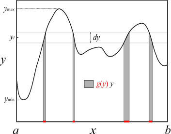
Figure 1: A schematic diagram showing the numerical integration notations. The red regions on the $x$-axis marked the portion within the interval $[a,b]$ that gives a certain value $y$. All the areas shaded in grey add up to give $g(y)y$.

We apply our algorithm to perform the following integration where the exact integral is known:

$$I=\int_{-2}^{2}x^{2}dx=\frac{16}{3}=5.33333\cdots,$$ (16)

and the “density of states” $g(y)$ can be expressed analytically:

$$g(y)=\frac{2(2-\sqrt{y})}{y}\hskip 14.22636pt\textrm{for $y>0$}.$$ (17)

We use a Fourier sine series as the basis set $\{\psi(E)\}$ to fit the remainder $R(E)$, and therefore a Fourier cosine series as the basis set $\{\phi(E)\}$ for constructing the correction $\ln c(E)$ and updating the density of states $\ln g(E)$. Moreover, we employ Kolmogorov-Smirnov test in the $R(E)$ fitting step to see if the expression obtained is a good fit to the dataset $\mathcal{D}$, using a criterion of $p=0.5$. The experiment is done for different numbers of data in the data set, with $k=$ 250, 500, 1000 and 2000.

We note that the Fourier sine and cosine series are not good basis sets for this problem due to their oscillatory properties. Yet the algorithm works surprisingly well. In Figure 2, we show a resulting density of states, $g(y)$, compared to that obtained using Wang-Landau sampling. The fluctuations of our $g(y)$ fall within the statistical noise of the WL density of states.

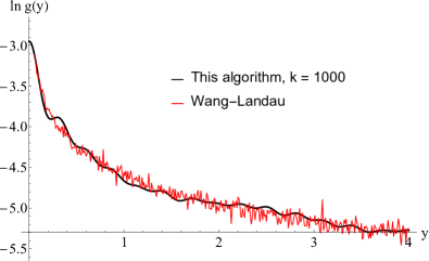
Figure 2: Density of states $g(y)$ at the $120^{\textrm{th}}$ iteration, obtained using 1000 data points in a data set (black curve), a total of $1.2\times 10^{5}$ MC steps are used. It is compared to a final $g(y)$ obtained using Wang-Landau sampling (red curve); this particular run requires $1.1\times 10^{6}$ MC steps to complete. The DOS obtained from our algorithm is significantly smoother, yet its fluctuations fall within the statistical noise of the Wang-Landau DOS.

The values of the estimated integral at different iterations for $k=500$ and $k=1000$ are shown in Figures 3 and 4, respectively.

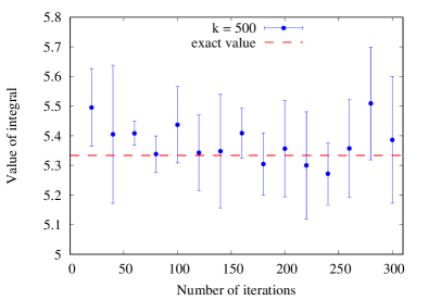
Figure 3: Integral of $x^{2}$ over $x\in[-2,2]$, obtained using 500 data points in a data set. Error bars are obtained from five independent runs.

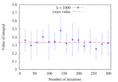
Figure 4: Integral of $x^{2}$ over $x\in[-2,2]$, obtained using 1000 data points in a data set. Error bars are obtained from five independent runs.

We observe that the number of data points $k$ in a data set within an iteration plays an important role in the accuracy. Both under-fitting from insufficient data and over-fitting from excessive data would produce inaccurate results. In both Figures 3 and 4, most estimated integrals agree with the exact value to within the error bars. No systematic correlation with the number of iterations is observed for both the estimated values of the integral and as well as the magnitude of the error bars. Using $k=500$ or $k=1000$ does not seem to result in significant differences in the estimated value of the integral. However, if we extend the studies and use fewer or more data points in the data set $\mathcal{D}$, we observe different behavior as shown in Figure 5. For the $k=250$ case, the integrals are slightly overestimated at the first 200 iterations or so. The percent errors fall back to within the same ranges as in the $k=500$ and $k=1000$ cases later. This is reasonable because as the number of iterations increases, more data are taken to correct the estimated density of states.

However, the integrals are, unexpectedly, systematically underestimated for the $k=2000$ case. We also observe that the number of terms in the expression of $R(E)$ and eventually $\ln g(E)$ generally increases with the number $k$ (Table 1). A larger number of data results in a more detailed fitting of the DOS, hence more terms are used in the construction of the correction. Unfortunately, there is also a higher risk of fitting the noise “too well”, causing an over-fitting of the estimated DOS. On the other hand, using too few data points (such as $k=250$) results in larger fluctuations in the values of the intergral as well as in the number of terms $N$ in the expression. From our observations, using about $k=1000$ data points in a data set is the safest and it strikes a good balance between under-fitting (or even mal-fitting) and overfitting.

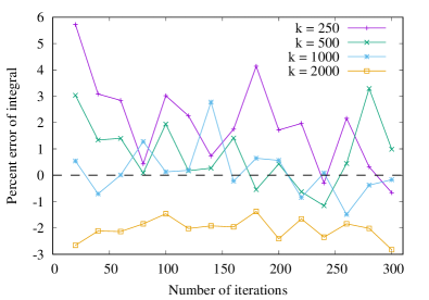
Figure 5: Percent errors of the averaged estimated integrals at different iterations using various numbers of data points $k$ in a data set. The integrals for all cases are averaged over five independent runs. Except for $k=2000$, all other cases converge to the exact value eventually with small errors (within $\pm 1\%$).

$k$	$N$
250	$19.4\pm 14.6$
500	$17.8\pm 6.1$
1000	$29.6\pm 4.3$
2000	$58.2\pm 13.0$

Table 1: Averaged number of basis functions ($N$) for different number of data points ($k$) in each data set. The average values and errors are obtained from five independent runs. The number $N$ is determined within the algorithm, at which the statistical test reaches $p\geq 0.5$.

Note that the above experiments complete within hundreds of iterations. Considering $k=1000$ data points in an iteration, the total number of MC steps needed is of the order of $10^{5}$. Comparing to the order of $10^{6}$ MC steps in Wang-Landau sampling, our scheme is more efficient and it saves about 10$\times$ MC steps. The reason is that when we correct the estimated DOS (i.e., sampling weights), the correction is constructed to drive the random walk intentionally to achieve uniform sampling, or a “flat histogram”, as opposed to an incremental correction using the histogram as in MUCA or WL sampling. We believe that our correction scheme can also be applied to simple models with discrete energy levels and yields significant speedup.

IV An improved scheme for better convergence

While the results above showed that our proposed scheme is successful, one problem is that it is still difficult to determine whether convergence has been reached. Here, we suggest a possible way to improve the quality of the results with two slight modifications to the original scheme.

Firstly, when determining the number of terms for the remainder $R(E)$ ($m$ in Eq. (8)), the original scheme starts from $m=1$ and increments it to $m+1$ sequentially until the statistical test gives a score of $p\geq 0.5$. We observe that this practice very often results in the update of the first few coefficients only. A remedy to it is that after the number $m$ is determined in the first iteration, in the later iterations we propose random permutations of the terms for the statistical test to start with. This way, every coefficient will have a roughly equal chance to get updated and refined.

Secondly, since the correction in Eq. (13) will drive the random walker in a way to achieve uniform sampling, we observe that it is beneficial to use a milder correction update to drive the random walker at a smaller step at a time. To do so, we rewrite Eq. (13) with a pre-factor $s$ to take only a portion of $R(E)$ as the correction:

$$\ln c(E) =s\sum_{i=1}^{m}r_{i}\frac{d\psi_{i}(E)}{dE}.$$ (18)

With these two small modifications, we revisited the integration problem using $k=1000$ data points in the data set (Figure 6). The integral values in the first few dozens of iterations deviate more from the exact value compared to the original scheme, but it converges slowly to the exact value with a much clearer convergence signal. In this example, one may terminate the simulation after e.g. the $150^{\textrm{th}}$ iteration. Another clear improvement is that the error bar for each final answer is much reduced compared to the original scheme, which indicates that the improved scheme is able to give more precise results.

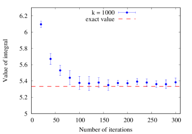
Figure 6: Integral of $x^{2}$ over $x\in[-2,2]$, obtained using 1000 data points in a data set and the improved scheme with a milder correction with the pre-factor $s=0.25$. Error bars are obtained from five independent runs.

V Further improvements

Our scheme is general in nature that the expression of the DOS $g(E)$ is not restricted to the Fourier form above, as long as there is a way to formulate the correction $c(E)$ and the update formula. Obviously, the quality of the resulting density of states depends heavily on the choice of a proper basis set. While the plane wave basis used in the present study allowed us to implement a prototype of our algorithm without major effort, it suffers from serious issues that will require the choice of more suitable basis sets. In particular, local improvements to the density of states in a limited region of the domain should not introduce changes in regions far away. Also, the density of states often spans a wide range of values; indeed the density of states for the integration example possesses a singularity at the domain boundary. Thus a more suitable, localized, basis set will greatly improve the convergence and accuracy of our method.

Although we present our method as a serial algorithm so far, we stress its parallelization is conceptually straight-forward. Since the generation of data points (which is the energy evaluations for a physical system) can be done independently by distributing the work over different processors, simple “poor-man’s” parallelization strategy would already guarantee significant speedup in both strong and weak scaling.

VI Conclusions

In this paper, we have presented a new Monte Carlo algorithm for calculating probability densities of systems with a continuous energy domain. The idea is inspired by combining ideas from the works of Wang and Landau Wang and Landau (2001b, a), Berg and Neuhaus Berg and Neuhaus (1991, 1992), as well as Berg and Harris Berg and Harris (2008). Nevertheless, our algorithm does not make use of an explicit histogram as in traditional Wang-Landau or multicanonical sampling. It is thus possible to avoid discrete binning of the collected data. This histogram-free approach allows us to obtain the estimated probability density, or the density of states, in terms of an analytic expression.

We have demonstrated the application of our algorithm to a stringent test case, numerical integration. Even with the sub-optimal Fourier sine and cosine basis sets, our current algorithm is already capable of giving reasonable results. An important point to note is that our algorithm requires much fewer number of Monte Carlo steps to finish a simulation. It is enabled by the novel way we proposed to correct the estimated density of states, and thus the sampling weights, where the random walk is directed consciously to achieve uniform sampling. This is essential for decreasing the time-to-solution ratio of a simulation, especially for complex systems where the computation time is dominated by energy evaluations.

The numerical integration test case provides useful insights into improving the algorithm. Possible improvements include the use of a basis set with local support and parallelization over energy calculations. Our ongoing work includes all the possibilities for perfecting the algorithm, as well as its application to simulations of physical systems to solve real-world scientific problems.

- (1)
- Bennett (1976) Charles H Bennett. 1976. Efficient estimation of free energy differences from Monte Carlo data. J. Comput. Phys. 22, 2 (1976), 245 – 268. https://doi.org/10.1016/0021-9991(76)90078-4
- Berg and Harris (2008) Bernd A. Berg and Robert C. Harris. 2008. From data to probability densities without histograms. Computer Physics Communications 179, 6 (Sept. 2008), 443–448. https://doi.org/10.1016/j.cpc.2008.03.010
- Berg and Neuhaus (1991) Bernd A. Berg and Thomas Neuhaus. 1991. Multicanonical algorithms for first order phase transitions. Physics Letters B 267, 2 (1991), 249 – 253. https://doi.org/10.1016/0370-2693(91)91256-U
- Berg and Neuhaus (1992) Bernd A. Berg and Thomas Neuhaus. 1992. Multicanonical ensemble: A new approach to simulate first-order phase transitions. Phys. Rev. Lett. 68 (Jan 1992), 9–12. Issue 1. https://doi.org/10.1103/PhysRevLett.68.9
- Eisenbach et al. (2009) Markus Eisenbach, Cheng-Gang Zhou, Don M. Nicholson, Greg Brown, Jeff Larkin, and Thomas C. Schulthess. 2009. A Scalable Method for Ab Initio Computation of Free Energies in Nanoscale Systems. In Proceedings of the Conference on High Performance Computing Networking, Storage and Analysis (SC ’09). ACM, New York, NY, USA, 64:1–64:8.
- Ferrenberg and Swendsen (1989) Alan M. Ferrenberg and Robert H. Swendsen. 1989. Optimized Monte Carlo data analysis. Phys. Rev. Lett. 63 (Sep 1989), 1195–1198. Issue 12. https://doi.org/10.1103/PhysRevLett.63.1195
- Hohenberg and Kohn (1964) Pierre Hohenberg and Walter Kohn. 1964. Inhomogeneous Electron Gas. Phys. Rev. 136, 3B (Nov. 1964), B864–B871. https://doi.org/10.1103/PhysRev.136.B864
- Hohenberg and Halperin (1977) Pierre C. Hohenberg and Bertrand I. Halperin. 1977. Theory of dynamic critical phenomena. Rev. Mod. Phys. 49 (Jul 1977), 435–479. Issue 3. https://doi.org/10.1103/RevModPhys.49.435
- Hukushima and Nemoto (1996) Koji Hukushima and Koji Nemoto. 1996. Exchange Monte Carlo method and application to spin glass simulations. Journal of the Physical Society of Japan 65, 6 (1996), 1604–1608.
- Khan and Eisenbach (2016) Suffian N. Khan and Markus Eisenbach. 2016. Density-functional Monte-Carlo simulation of CuZn order-disorder transition. Phys. Rev. B 93 (Jan 2016), 024203. Issue 2. https://doi.org/10.1103/PhysRevB.93.024203
- Kohn and Sham (1965) Walter Kohn and Lu Jeu Sham. 1965. Self-Consistent Equations Including Exchange and Correlation Effects. Phys. Rev. 140, 4A (Nov. 1965), A1133–A1138. https://doi.org/10.1103/PhysRev.140.A1133
- Landau and Binder (2015) David P. Landau and Kurt Binder. 2015. A Guide to Monte Carlo Simulations in Statistical Physics, 4th Edition. Cambridge University Press, Cambridge, U.K.
- Li et al. (2007) Ying Wai Li, Thomas Wüst, David P. Landau, and Hai-Qing Lin. 2007. Numerical integration using Wang-Landau sampling. Computer Physics Communications 177, 6 (Sept. 2007), 524–529. https://doi.org/10.1016/j.cpc.2007.06.001
- Metropolis et al. (1953) Nicholas Metropolis, Arianna W. Rosenbluth, Marshall N. Rosenbluth, Augusta H. Teller, and Edward Teller. 1953. Equation of State Calculations by Fast Computing Machines. The Journal of Chemical Physics 21, 6 (1953), 1087–1092. https://doi.org/10.1063/1.1699114
- Swendsen and Wang (1986) Robert H. Swendsen and Jian-Sheng Wang. 1986. Replica Monte Carlo Simulation of Spin-Glasses. Phys. Rev. Lett. 57 (Nov 1986), 2607–2609. Issue 21. https://doi.org/10.1103/PhysRevLett.57.2607
- Torrie and Valleau (1977) G.M. Torrie and J.P. Valleau. 1977. Nonphysical sampling distributions in Monte Carlo free-energy estimation: Umbrella sampling. J. Comput. Phys. 23, 2 (1977), 187 – 199. https://doi.org/10.1016/0021-9991(77)90121-8
- Vogel et al. (2013) Thomas Vogel, Ying Wai Li, Thomas Wüst, and David P. Landau. 2013. Generic, Hierarchical Framework for Massively Parallel Wang-Landau Sampling. Phys. Rev. Lett. 110 (May 2013), 210603.
- Vogel et al. (2014) Thomas Vogel, Ying Wai Li, Thomas Wüst, and David P. Landau. 2014. Scalable replica-exchange framework for Wang-Landau sampling. Phys. Rev. E 90 (Aug 2014), 023302. Issue 2. https://doi.org/10.1103/PhysRevE.90.023302
- Wang and Landau (2001a) Fugao Wang and David P. Landau. 2001a. Determining the density of states for classical statistical models: A random walk algorithm to produce a flat histogram. Phys. Rev. E 64 (Oct 2001), 056101. Issue 5. https://doi.org/10.1103/PhysRevE.64.056101
- Wang and Landau (2001b) Fugao Wang and David. P. Landau. 2001b. Efficient, Multiple-Range Random Walk Algorithm to Calculate the Density of States. Phys. Rev. Lett. 86 (Mar 2001), 2050–2053. Issue 10. https://doi.org/10.1103/PhysRevLett.86.2050
- Yin and Landau (2012) Junqi Yin and David P. Landau. 2012. Massively parallel Wang-Landau sampling on multiple {GPUs}. Computer Physics Communications 183, 8 (2012), 1568 – 1573. https://doi.org/10.1016/j.cpc.2012.02.023
- Zierenberg et al. (2013) Johannes Zierenberg, Martin Marenz, and Wolfhard Janke. 2013. Scaling properties of a parallel implementation of the multicanonical algorithm. Computer Physics Communications 184, 4 (2013), 1155 – 1160. https://doi.org/10.1016/j.cpc.2012.12.006