Distribution of the Dirac modes in QCD

Abstract

It was established that distribution of the near-zero modes of the Dirac operator is consistent with the Chiral Random Matrix Theory (CRMT) and can be considered as a consequence of spontaneous breaking of chiral symmetry (SBCS) in QCD. The higher-lying modes of the Dirac operator carry information about confinement physics and are not affected by SBCS. We study distributions of the near-zero and higher-lying modes of the overlap Dirac operator within $N_{F}=2$ dynamical simulations. We find that distributions of both near-zero and higher-lying modes are the same and follow the Gaussian Unitary Ensemble of Random Matrix Theory. This means that randomness, while consistent with SBCS, is not a consequence of SBCS and is related to some more general property of QCD in confinement regime.

1 Introduction

The near-zero modes of the Dirac operator in QCD are related to spontaneous breaking of chiral symmetry (SBCS) via the Banks-Casher relation BANKS1980103 . On the lattice with a finite volume they are subject to some universal behaviour PhysRevD.46.5607 . Within the $\epsilon$-regime, i.e. when $\Lambda_{QCD}L\gg 1$ and $m_{\pi}L\ll 1$, where $L$ is the linear size of the lattice and $m_{\pi}$ is the pion mass, the Chiral Random Matrix Theory (CRMT) links the distribution law of the near-zero modes of the Dirac operator with the random matrices SHURYAK1993306 ; 537280920001201 .

With $N_{F}$ degenerate quark flavors of mass $m$ the Dirac operator in the Weyl representation of $\gamma$-matrices can be written as

$$D=\left(\begin{matrix}m&iW\\ iW^{+}&m\end{matrix}\right).$$ (1)

The distribution of the large matrix $W$ with dimension determined by the lattice size, is given by

$$P(W)=\mathcal{N}det(D)^{N_{f}}e^{-\frac{N\beta\Sigma^{2}}{4}tr(W^{\dagger}W)},$$ (2)

where $\mathcal{N}$ is the normalization constant, $\Sigma$ is a parameter that it is not always related to the chiral condensate (not - if we are beyond the $\epsilon$ regime), and $\beta$ is the Dyson index which is determined by the symmetry properties of the matrix $W$. For different values of $\beta$ we have different matrix ensembles. If $\beta=1$ we have the Gaussian Orthogonal Ensemble (GOE), if $\beta=2$ the Gaussian Unitary Ensemble (GUE) and $\beta=4$, the Gaussian Symplectic Ensemble (GSE). In QCD $\beta=2$ as was shown in Ref. PhysRevLett.72.2531 .

Given eq. (2) properties of the near-zero modes in QCD are connected with properties of large random matrices. The near-zero mode distribution has been studied on the lattice in many papers, see e.g. PhysRevD.76.054503 , and a perfect agreement with the CRMT has been found.

While the lowest-lying modes of the Dirac operator are strongly affected by SBCS, the higher-lying modes are subject to confinement physics. This was recently observed on the lattice via truncation of the lowest modes of the overlap Dirac operator from quark propagators PhysRevD.89.077502 ; PhysRevD.91.034505 ; PhysRevD.91.114512 ; PhysRevD.92.099902 . Hadrons survive this truncation (except for pion) and their mass remains large. It was noticed that not only $SU(2)_{L}\times SU(2)_{R}$ and $U(1)_{A}$ chiral symmetries get restored, but actually some higher symmetry appears. This symmetry was established to be $SU(2)_{CS}$ (chiral-spin) and $SU(4)$ that contains chiral symmetries as subgroups and that is a symmetry of confining chromo-electric interaction Glozman2015 ; PhysRevD.92.016001 . Given lattice size $L\sim 2$ fm in refs. PhysRevD.89.077502 ; PhysRevD.91.034505 ; PhysRevD.91.114512 ; PhysRevD.92.099902 it was enough to remove lowest 10-20 modes of the Dirac operator to observe emergence of $SU(2)_{CS}$ and $SU(4)$. Consequently the higher-lying modes, that are above the lowest 10-20 modes, are not affected by SBCS and by breaking of $U(1)_{A}$ and carry information about confinement as well as about $SU(2)_{CS}$ and $SU(4)$ symmetries.

Given success of CRMT for the lowest-lying modes of the Dirac operator it is natural to expect that distribution law of the higher-lying modes should be different and should reflect confinement physics. This motivates our study of the distribution of the lowest-lying and higher-lying modes of the Dirac operator and their comparison.

2 Lattice setup

We compute 200 lowest eigenvalues of the overlap Dirac operator Ref. NEUBERGER1998141 ; NEUBERGER1998353 defined as

$$D_{ov}(m)=\left(\rho+\frac{m}{2}\right)+\left(\rho-\frac{m}{2}\right)\gamma^{5}sign[H(-\rho)],$$ (3)

where $H(-\rho)=\gamma^{5}D(-\rho)$ and $D(-\rho)$ is the Wilson-Dirac operator; $m=0.015$ is the valence quarks mass and $\rho=1.6$ is a simulation parameter. We use 100 gauge field configurations in the zero topological sector generated by JLQCD collaboration with $N_{f}=2$ dynamical overlap fermions on a $L^{3}\times L_{t}=16^{3}\times 32$ lattice with $\beta=2.30$ and lattice spacing $a\sim 0.12fm$. The pion mass is $m_{\pi}=289(2)MeV$, see Ref. PhysRevD.78.014508 ; doi:10.1093/ptep/pts006 ; PhysRevLett.101.202004 . Precisely the same gauge configurations have been used in truncation studies PhysRevD.89.077502 ; PhysRevD.91.034505 ; PhysRevD.91.114512 ; PhysRevD.92.099902 .

We point out that with this lattice setup we are not in the $\epsilon$-regime, because $m_{\pi}L\simeq 3$. Therefore it is not a priori obvious that CRMT will work also in our case.

To obtain the eigenvalues $\lambda_{ov}(m)$ of $D_{ov}(m)$ we first calculate the sign function $sign[H]$. We use the Chebyshev polynomials to approximate $sign[H]$ with an accuracy of $\epsilon=10^{-18}$, and then compute $200$ eigenvalues of $D_{ov}(m)$. For our analysis we consider only the eigenvalues with $Im(\lambda_{ov}(m))\geq 0$ because we know from the Ginsparg-Wilson equation $\{\gamma^{5},D_{ov}(0)\}=\frac{1}{\rho}D_{ov}(0)\gamma^{5}D_{ov}(0)$ and the $\gamma^{5}$-hermiticity, i.e. $D_{ov}^{\dagger}(0)=\gamma^{5}D_{ov}(0)\gamma^{5}$, that the eigenvalues come in pairs $(\lambda_{ov}(m),\lambda_{ov}^{*}(m))$. Therefore the eigenvalues below the real axis bring the same information as the eigenvalues above the real axis.

The eigenvalues of the overlap Dirac operator lie on a circle with radius $R=\rho-\frac{m}{2}$, see Fig. 1. Therefore in order to recover chiral symmetry for the massless Dirac operator in continuum theory we need to project our eigenvalues on the imaginary axis. In principle there is not an unique way to do this. Hence we use three different projections that define the eigenvalues in continuum limit. All these three definitions are illustrated on Fig. 1. We will study sensitivity of our results on choice of projection definition.

(a) $\lambda=\frac{Im\>\lambda_{ov}(m)}{1-\frac{Re\>\lambda_{ov}(m)}{\rho+\frac{m}{2}}}$

(b) $\lambda=\frac{Im\>\lambda_{ov}(m)}{1-\frac{Re\>\lambda_{ov}(m)}{2\rho}}$

(c) $\lambda=\left(\rho-\frac{m}{2}\right)\theta$

Figure 1: Different definitions of $\lambda$ using the eigenvalues of the overlap Dirac operator, $\lambda_{ov}(m)$. The angle $\theta$ is defined as $\theta=arctg\left(\frac{Im\>\lambda_{ov}(m)}{\left(\rho+\frac{m}{2}\right)-Re\>\lambda_{ov}(m)}\right)$.

3 Lowest eigenvalues

First we study the lowest eigenvalues of the Dirac operator. We are not in the $\epsilon$-regime so we don’t expect a priori a full agreement with CRMT. Consequently we want to check whether and to what extent the lowest eigenvalues are described by CRMT.

An important prediction of CRMT is the distribution of the lowest eigenvalues in the thermodynamic limit. It means in the limit when the four dimensional volume of our lattice $V\rightarrow\infty$ and the quantity $V\Sigma m_{\pi}$ is fixed.

Defining the variables $\zeta_{k}=V\Sigma\lambda_{k}$, where, in our case, $\lambda_{k}$ is the $k$-th lowest projected eigenvalue of the overlap Dirac operator, then we can get (see Ref. PhysRevD.63.045012 ) the distribution $p_{k}(\zeta_{k})$ of each $\zeta_{k}$.

Since we don’t know the parameter $\Sigma$ we study the ratios $\langle\lambda_{k}\rangle/\langle\lambda_{j}\rangle$, where $\langle\lambda_{i}\rangle$ is the average over all gauge configurations for the $i$th projected eigenvalue. Indeed using that $\langle\zeta_{k}\rangle=V\Sigma\langle\lambda_{k}\rangle$, we can compare our ratios with the predictions of CRMT. We show the data for $1\leq j<k\leq 4$ in Table 1 and in the last column there are the values predicted by CRMT.

Table 1: Ratio $\langle\lambda_{k}\rangle/\langle\lambda_{j}\rangle$ for $1\leq j\leq k\leq 4$ and the same values computed with the CRMT. We denote with $\sigma$ the error. In this case we have used $\lambda$ defined as in Fig. 1(b).

$k/j$	$\langle\lambda_{k}\rangle/\langle\lambda_{j}\rangle$	$\sigma$	CRMT
2/1	2.72	0.19	2.70
3/1	4.35	0.28	4.46
3/2	1.60	0.06	1.65
4/1	5.92	0.38	6.22
4/2	2.17	0.08	2.30
4/3	1.36	0.03	1.40

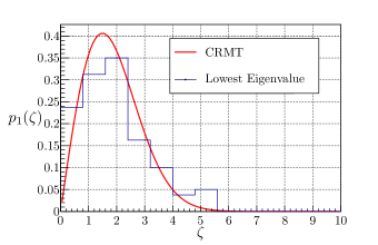
Figure 2: Distribution of the lowest eigenvalue. In this case $\zeta=V\Sigma\lambda$.

We can see that the ratios for the first $3$ projected eigenvalues are in good agreement with the CRMT. The ratios involving the $4$-th projected eigenvalues have a larger discrepancy.

From the theoretical values of $\langle\zeta_{k}\rangle$ and the observed values of $\langle\lambda_{k}\rangle$ we can get the parameter $\Sigma$. We find for our system that $\Sigma=(232.2\pm 0.9MeV)^{3}$. We use this parameter to compare the distribution of the first lowest projected eigenvalue with the theoretical distribution given by CRMT, as we report in Fig. 2.

We can conclude this section observing that, even if we are not in the $\epsilon$-regime, for very low eigenvalues in our system the predictions of CRMT still work.

4 Nearest neighbor spacing distribution

Another important prediction of CRMT is the nearest neighbor spacing distribution (or NNS distribution). This is the distribution of the variable

$$s_{n}=\xi_{n+1}-\xi_{n},$$

where

$$\xi_{n}=\xi(\lambda_{n})=\int_{0}^{\lambda_{n}}R(\lambda)d\lambda$$

and $R(\lambda)d\lambda$ is the probability to find an eigenvalue of the Dirac operator in the interval $(\lambda,\lambda+d\lambda)$. $n$ indicates the number of the lowest projected eigenvalue, supposing we have ordered the projected eigenvalues such that $\lambda_{1}\leq\lambda_{2}\leq...\leq\lambda_{n}$. In principle we don’t know how $R(\lambda)$ is made and the procedure to map the set of variables $\{\lambda_{1},...,\lambda_{n}\}$ into the set $\{\xi_{1},...,\xi_{n}\}$ is called unfolding and it is described in Guhr1998189 . This procedure is based on the introduction of the following variable

$$\eta(\lambda_{n})=\int_{0}^{\lambda_{n}}\rho(\lambda)d\lambda=\frac{1}{N}\langle\sum_{k}\theta(\lambda_{n}-\lambda_{k})\rangle=\frac{1}{N}\frac{1}{M}\sum_{i=1}^{M}\sum_{k}\theta(\lambda_{n}-\lambda_{k}^{i}),$$

where $\rho(\lambda)=\frac{1}{N}\langle\sum_{k}\delta(\lambda-\lambda_{k})\rangle$ is the spectral density of the Dirac operator averaged over all gauge field configurations, $\lambda_{k}^{i}$ denotes the $k$th lowest projected eigenvalue of the Dirac operator computed using the $i$th gauge configuration. $M=100$ is the number of gauge configurations that we are taking into account and $N$ is total number of the eigenvalues of the Dirac operator. Now $\eta(\lambda)$ can be decomposed in a fluctuating part $\eta_{fl}(\lambda)$ and in a smooth part $\xi(\lambda)$, namely $\eta(\lambda)=\xi(\lambda)+\eta_{fl}(\lambda)$. The smooth part $\xi(\lambda)$ can be obtained by a polynomial fit of $\eta(\lambda)$.

For different values of the Dyson index $\beta$ we have different shapes for the NNS distribution.

We use this distribution to study the lowest and higher eigenvalues of the overlap Dirac operator. The lowest eigenvalues contain the information about the $SU(2)_{L}\otimes SU(2)_{R}$ and $U(1)_{A}$ breakings. The NNS distribution calculated with 10 lowest Dirac eigenmodes is shown in the left panel of Fig. 3. We see that the distribution is perfectly described by the Gaussian Unitary Ensemble, in agreement with CRMT.

The right panel of Fig. 3 shows NNS distribution obtained with eigenmodes in the interval 81 - 100. It is clear from results of refs. PhysRevD.89.077502 ; PhysRevD.91.034505 ; PhysRevD.91.114512 ; PhysRevD.92.099902 that this part of the Dirac spectrum is not sensitive to SBCS and to breaking of $U(1)_{A}$, but reflect physics of confinement and of $SU(2)_{CS}$ and $SU(4)$ symmetries. Nevertheless, distribution of these eigenmodes of the Dirac operator is described by the same Wigner distribution (GUE) as of the lowest ten modes, which is unexpected.

Finally, in Fig. 4 we show NNS distributions of the lowest 100 modes calculated with three different definitions of projected eigenvalue, compare with Fig. 1. It is clear that results for distribution is not sensitive to definition of projected eigenvalue.

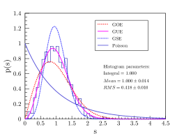
(a) Range eigenvalues: 1 - 10

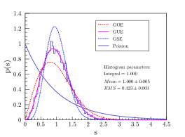
(b) Range eigenvalues: 81 - 100

Figure 3: NNS distribution for the first $10$ lowest projected eigenvalues of the overlap Dirac operator on the left, and the higher eigenvalues on the right. We have used $\lambda$ defined as in Fig. 1(b).

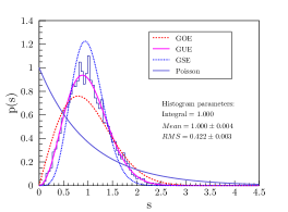
(a) $\lambda=\frac{Im\>\lambda_{ov}(m)}{1-\frac{Re\>\lambda_{ov}(m)}{\rho+\frac{m}{2}}}$

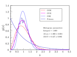
(b) $\lambda=\frac{Im\>\lambda_{ov}(m)}{1-\frac{Re\>\lambda_{ov}(m)}{2\rho}}$

(c) $\lambda=\left(\rho-\frac{m}{2}\right)\theta$

Figure 4: NNS distribution for the lowest $100$ eigenvalues of the Dirac operator, for different definitions of $\lambda$.

5 Conclusions

In this work we have analyzed distributions of the lowest and the higher-lying eigenvalues of the overlap Dirac operator. We have seen that the lowest eigenvalues are well described by CRMT in agreement with previous studies.

We have also studied the nearest neighbor spacing distribution for the higher eigenvalues that are affected neither by $U(1)_{A}$ breaking nor by spontaneous breaking of chiral symmetry. These modes are sensitive to confinement physics and to related $SU(2)_{CS}$ and $SU(4)$ symmetries. We have found that they follow the Wigner distribution as the near-zero modes. This observation means that the Wigner distribution seen both for the near-zero and higher-lying modes, while consistent with spontaneous breaking of chiral symmetry, is not a consequence of spontaneous breaking of chiral symmetry in QCD but has some more general origin in QCD in confinement regime. In other words a randomness that we observe both for the near-zero modes and for the higher-lying modes has not yet known origin in QCD.

Acknowledgments

We thank C.B. Lang for numerous discussions. This work is supported by the Austrian Science Fund FWF through grants DK W1203-N16 and P26627-N27.

References

- (1) T. Banks, A. Casher, Nucl.Phys. B169, 103 (1980)
- (2) H. Leutwyler, A. Smilga, Phys.Rev. D46, 5607 (1992)
- (3) E. Shuryak, J. Verbaarschot, Nucl.Phys. A560, 306 (1993)
- (4) J. Verbaarschot, T. Wettig, Ann.Rev.Nucl.Part.Sci. 50, 343 (2000)
- (5) J. Verbaarschot, Phys.Rev.Lett. 72, 2531 (1994)
- (6) H. Fukaya, S. Aoki, T.W. Chiu, S. Hashimoto, T. Kaneko, H. Matsufuru, J. Noaki, K. Ogawa, T. Onogi, N. Yamada (JLQCD Collaboration and TWQCD Collaboration), Phys.Rev. D76, 054503 (2007)
- (7) M. Denissenya, L.Y. Glozman, C.B. Lang, Phys.Rev. D89, 077502 (2014)
- (8) M. Denissenya, L.Y. Glozman, C.B. Lang, Phys.Rev. D91, 034505 (2015)
- (9) M. Denissenya, L.Y. Glozman, M. Pak, Phys.Rev. D91, 114512 (2015)
- (10) M. Denissenya, L.Y. Glozman, M. Pak, Phys.Rev. D92, 099902 (2015)
- (11) L.Y. Glozman, Eur.Phys.J. A51, 27 (2015)
- (12) L.Y. Glozman, M. Pak, Phys.Rev. D92, 016001 (2015)
- (13) H. Neuberger, Phys.Lett. B417, 141 (1998)
- (14) H. Neuberger, Phys.Lett. B427, 353 (1998)
- (15) S. Aoki, H. Fukaya, S. Hashimoto, K.I. Ishikawa, K. Kanaya, T. Kaneko, H. Matsufuru, M. Okamoto, M. Okawa, T. Onogi et al. (JLQCD Collaboration), Phys.Rev. D78, 014508 (2008)
- (16) S. Aoki, T.W. Chiu, G. Cossu, X. Feng, H. Fukaya, S. Hashimoto, T.H. Hsieh, T. Kaneko, H. Matsufuru, J.I. Noaki et al., PTEP 2012, 01A106 (2012)
- (17) J. Noaki, S. Aoki, T.W. Chiu, H. Fukaya, S. Hashimoto, T.H. Hsieh, T. Kaneko, H. Matsufuru, T. Onogi, E. Shintani et al. (JLQCD and TWQCD Collaborations), Phys.Rev.Lett. 101, 202004 (2008)
- (18) P.H. Damgaard, S.M. Nishigaki, Phys.Rev. D63, 045012 (2001)
- (19) T. Guhr, A. MÃllerâGroeling, H.A. WeidenmÃller, Phys.Rep. 299, 189 (1998)