Transport of hot carriers in plasmonic nanostructures

Abstract

Plasmonic hot carrier devices extract excited carriers from metal nanostructures before equilibration, and have the potential to surpass semiconductor light absorbers. However their efficiencies have so far remained well below theoretical limits, which necessitates quantitative prediction of carrier transport and energy loss in plasmonic structures to identify and overcome bottlenecks in carrier harvesting. Here, we present a theoretical and computational framework, Non-Equilibrium Scattering in Space and Energy (NESSE), to predict the spatial evolution of carrier energy distributions that combines the best features of phase-space (Boltzmann) and particle-based (Monte Carlo) methods. Within the NESSE framework, we bridge first-principles electronic structure predictions of plasmon decay and carrier collision integrals at the atomic scale, with electromagnetic field simulations at the nano- to mesoscale. Finally, we apply NESSE to predict spatially-resolved energy distributions of photo-excited carriers that impact the surface of experimentally realizable plasmonic nanostructures at length scales ranging from tens to several hundreds of nanometers, enabling first-principles design of hot carrier devices.

Surface plasmon resonances shrink optics to the nano scale, facilitating strong focusing and localized absorption of light Altewischer et al. (2002); Gramotnev and Bozhevolnyi (2010); Atwater and Polman (2010); Schuller (2010); Brongersma et al. (2015). Decay of plasmons generates energetic electrons and holes in the material that can be exploited for applications including photodetection, imaging and spectroscopy Takahashi and Tatsuma (2011); Wang and Melosh (2011); Jang et al. (2018); Hobbs et al. (2017); Schuck (2013); Adleman et al. (2009); Awazu (2008), photonic energy conversion, and photocatalysis Brus (2008); Christopher et al. (2011); Chen et al. (2011); Cushing and Wu (2013); Frischkorn and Wolf (2006); Wu et al. (2015). However, these applications require carriers that retain a significant fraction of their energy absorbed from the plasmon, which is typically two orders of magnitude larger than the thermal energy scale. Experimentally, the energy distributions of hot carriers that critically impact their efficiency of collection cannot be measured directly, but must instead be inferred indirectly from optical response in pump-probe measurements,Inouye et al. (1998); Furube et al. (2007); Harutyunyan et al. (2015) from photo-current measurements,Knight et al. (2011); Zheng et al. (2015) or from redox-reaction chemical markers.Buntin et al. (1988) This critically necessitates theoretical prediction of charge transport in metal nanostructures far from equilibrium, which presents a major challenge for current computational methods Ziman (1964); Chen and Tao (2009); Del Fatti et al. (2000); Tame et al. (2013).

In extremely small nano-scale systems, electron dynamics require a full quantum mechanical treatment, and several classes of techniques have been developed for quantum transport simulations. In diagrammatic many-body perturbation theory, quantum transport can be described using the non-equilibrium Greens function (NEGF) formalism Stefanucci and van Leeuwen (2013), which has been applied extensively to electron transport in molecular junctions Thoss and Evers (2018). atoms in rarefied gases Perfetto et al. (2015), nanoscale metal interconnects Zhou et al. (2018), and small plasmonic nanoparticles Zhang et al. (2016). Open quantum system approaches applied to photons have similarly enabled efficient prediction of retardation and radiative effects on plasmon resonances of nanostructures Downing et al. (2017a, b). Correspondingly, within the density-functional formalism, time-dependent density-functional theory (TD-DFT) Runge and Gross (1984) and simplified non-adiabatic molecular dynamics (NAMD) Wang et al. (2015) simulations have also been used to describe electron transport in molecules Stephan ; Stefanucci and Almbladh (2004), at material interfaces Long and Prezhdo (2014); Wang et al. (2016), and in small plasmonic nanoparticles Manjavacas et al. (2014); Ma et al. (2015). Both NEGF and TD-DFT methods can been applied to systems approaching tens of nanometers in dimension using simplified free-electron-like models. However, in first principles simulations retaining detailed electronic structure information, these techniques are limited by computational complexity to at most a few hundred atoms, corresponding to dimensions of a few nanometers.

Plasmonic nanostructures designed for harvesting hot carriers typically range from ten to several hundred nanometers in dimensions, well beyond dimensions where quantum transport simulations would be practical. Additionally, with increasing dimensions, classical transport becomes a better approximation, appropriate for hot carrier transport in these devices. Classical transport methods include stochastic approaches that track dynamics of individual particles, and probabilistic approaches that describe the evolution of distribution functions. The Boltzmann transport equation, of the latter kind, is still computationally intensive in its most general form because it requires tracking probability distributions in a six-dimensional phase space of spatial and momentum degrees of freedom Golovchenko (1976); Hagelaar and Pitchford (2005). Conventional simplifications of the Boltzmann equation include restriction of the space of allowed distribution functions, or simplified collision integrals such as the relaxation-time approximation Guyer and Krumhansl (1966); Chen (2001); Mermin (1970). but these neglect key electronic structure details critical in plasmonic hot carrier transport. On the other hand, stochastic approaches such as Monte Carlo (MC) simulations Binder (1986) introduce significant computational advantages for simple models of collisions, but they become much more computationally demanding for a complex collision model such as one based on electronic structure theory.

We have previously shown the importance of describing hot carrier generation and transport in plasmonic materials with full electronic structure details in the densities of states of carriers and their matrix elements for optical transitions and interactions with phonons Sundararaman et al. (2014); Brown et al. (2015). Neglecting spatial transport, we have combined these calculations with simplified Boltzmann equation solutions to elucidate non-equilibrium effects in the ultrafast spectroscopy of small plasmonic nanoparticles Brown et al. (2016, 2017). However, capturing the spatial variation of carrier distributions is critical in larger and more complex plasmonic nanostructures, where carrier generation is strongly inhomogeneous and often localized near electromagnetic hot spots Cortes et al. (2017); Tagliabue et al. (2018). Simultaneously capturing electronic structure details with spatial transport in realistic plasmonic nanostructures has so far remained a challenge.

In this Article, we present a hybrid computational framework for efficiently describing non-equilibrium classical charge transport that combines the advantages of the probabilistic and stochastic approaches. In section I, we derive this Non-Equilibrium Scattering in Space and Energy (NESSE) framework as a limit of the Boltzmann equation by tracking distribution functions indexed by number of collisions, under the assumption of momentum randomization at each collision. We then specialize the general NESSE approach to plasmonic hot carriers in section II, linked with first-principles calculations of carrier generation and scattering, as well as electromagnetic field simulations. In section IV, we use NESSE to predict the spatially-resolved energy distributions of hot carriers that reach the surface in metal nanostructures of various materials and geometries up to several hundred nanometers in dimensions, simultaneously accounting for electronic structure detail and nanoscale geometry. These spatially-resolved hot carrier energy distributions are vital to understand optical, electronic or chemical signatures of hot carriers in experiments, and provide a direct mechanistic understanding of the transport and energy relaxation effects which are only indirectly measurable experimentally.

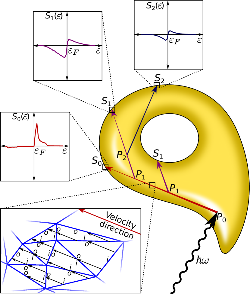
Figure 1: Non-Equilibrium Scattering in Space and Energy (NESSE) framework for evaluating non-equilibrium carrier transport in plasmonic nanostructures. Electromagnetic field simulations and first-principles calculations of plasmon decay determine the spatially-resolved initial carrier distribution, $P_{0}$. Tracing the distributions using ab-initio calculated mean free paths and collision integrals determines the collected surface flux before scattering $S_{0}$, and the distribution of carriers after one scattering event $P_{1}$. Repeating this process yields energy-resolved carrier fluxes after fixed numbers of scattering events $S_{0}$, $S_{1}$, $S_{2}$ etc. (upper insets). Propagation of carrier distributions between scattering events is calculated efficiently on a tetrahedral discretization of the nanostructure geometry (bottom inset). NESSE effectively solves the linearized Boltzmann equation simultaneously for the spatial and energy distributions of carriers, assuming momentum is randomized at each scattering event, in structures with arbitrary geometry and topology, as illustrated by the arbitrarily complex shape chosen above.

I Computational Framework (NESSE)

The general goal of non-equilibrium transport calculations is to predict the distribution of particles in phase space, i.e. with spatial as well as momentum resolution, accounting for sources of particles and the various scattering mechanisms between particles. For example, for plasmonic hot carrier devices we need to predict the usable carrier distribution that reaches the surface above a threshold energy, starting from the initial distribution generated by plasmon decay and accounting for electron-electron, electron-phonon and surface scattering in the material. Such devices are typically operated under constant illumination, where carriers are being generated at a constant rate. This results in steady-state time-independent carrier energy distributions, while we are interested primarily in the far-from-equilibrium hot-carrier component of these energy distributions (far from the Fermi level). Additionally, in most cases, the number of hot carriers excited is a small fraction of the number of electrons in the plasmonic metal, such that hot carriers predominantly scatter against thermal carriers, enabling a linearization of the transport equations as we discuss below. Hence, in this work, we focus on far-from-equilibrium transport in the linearized steady-state limit, which is the predominant regime for hot-carrier solar energy harvesting.

In steady state, the general transport problem is described by the time-independent Boltzmann equation,

$$\boldsymbol{\mathbf{v}}_{s}\cdot\nabla f(s,\boldsymbol{\mathbf{r}})=P_{0}(s,\boldsymbol{\mathbf{r}})+\Gamma_{s}[f],$$ (1)

in terms of the spatially-varying state occupation $f(s,\boldsymbol{\mathbf{r}})$. The abstract state label $s$ includes all degrees of freedom at a given point in space, which is just momentum $\boldsymbol{\mathbf{p}}$ in the classical case. For electrons in a material, $s$ combines crystal momentum $\boldsymbol{\mathbf{k}}$ in the Brillouin zone with a band index $n$.

The term on the left side of (1) accounts for drift of particles in state $s$ with velocity $\boldsymbol{\mathbf{v}}_{s}$. The first term on the right side, $P_{0}$, accounts for particle generation, while the second term, the collision integral $\Gamma$ accounts for scattering. See section II for a complete specification of these terms for the plasmonic hot carrier example starting from the electronic structure of the material.

Once the source term and collision integrals have been defined, the Boltzmann equation is fully specified and can, in principle, be solved. However, this deceptively simple-looking equation is a nonlinear integro-differential equation in six dimensions, differential in the three spatial dimensions $\boldsymbol{\mathbf{r}}$ and integral (non-local) in the three momentum dimensions in $\boldsymbol{\mathbf{k}}$ within $s$, which makes it extremely expensive computationally. The remainder of this section develops a practical approximation to this equation that is suited for analyzing hot carrier transport and related scenarios.

The first substantial simplification is linearization of the collision integral, which is possible whenever the particles in which we are interested in scatter predominantly against a background of particles whose distribution is fixed or already known. For plasmonic hot carriers, this is the case in the low intensity regime, where the number of excited far-from-equilibrium carriers is small compared to the background of equilibrium carriers. In this regime, hot carriers scatter predominantly against equilibrium carriers, and phonons remain approximately in equilibrium at the ambient temperature $T_{0}$. We can then separate $f(s,\boldsymbol{\mathbf{r}})=f_{0}(\varepsilon_{s},T_{0})+\phi(s,\boldsymbol{\mathbf{r}})$, where the first term is the equilibrium (Fermi) distribution, and the second term is the deviation from equilibrium. Substituting this into (1), Taylor expanding the collision integral about the equilibrium Fermi distribution $f_{0}$, and dropping terms at second order and higher in $\phi(s,\boldsymbol{\mathbf{r}})$ yields the linearized steady-state Boltzmann equation,

$$\boldsymbol{\mathbf{v}}_{s}\cdot\nabla\phi(s,\boldsymbol{\mathbf{r}})=P_{0}(s,\boldsymbol{\mathbf{r}})+\sum_{s^{\prime}}C_{ss^{\prime}}\phi(s^{\prime},\boldsymbol{\mathbf{r}}),$$ (2)

where the ‘collision matrix’ $C$ arises from the first order term in the Taylor expansion of the collision integral,

$$C_{ss^{\prime}}=\left.\frac{\partial\Gamma_{s}[f]}{\partial f(s^{\prime})}\right|_{f=f_{0}}.$$ (3)

The zeroth order terms in this equation, which correspond to the equilibrium configuration, cancel by definition. Above and henceforth, any sum over a state index $s$ is understood to imply integration over the continuous $\boldsymbol{\mathbf{k}}$ degrees of freedom contained within.

Importantly, while the collision integral $\Gamma[f(s,\boldsymbol{\mathbf{r}})]$ varies spatially due to the spatial dependence of $f(s,\boldsymbol{\mathbf{r}})$, the collision matrix does not. In the hot carrier case, linearization is only valid for energies several $k_{B}T$ away from the Fermi level because electron-electron scattering produces more low-energy carriers, eventually affecting all electrons near the Fermi energy in the material, regardless of the incident intensity and initial number of carriers. Assuming linearity (inherently an approximation) is adequate for analyzing plasmonic hot carrier devices, but retaining the nonlinearity is important for describing the thermalized regime and, of course, for high-intensity regimes explored in ultrafast spectroscopy, which we have analyzed in detail elsewhere (neglecting spatial dependence instead in that case) Brown et al. (2016, 2017).

The linearized steady-state Boltzmann equation (2) remains extremely challenging to solve since it still requires keeping track of a six-dimensional distribution function. In order to address this issue, we rearrange the equation to separate the distribution functions by the number of scattering events. First, we separate the diagonal terms of the scattering matrix, which correspond to the state inverse-lifetimes $\tau_{s}^{-1}$, to write

$$C_{ss^{\prime}}\equiv-\tau_{s}^{-1}\delta_{ss^{\prime}}+M_{ss^{\prime}}$$ (4)

and thereby define the ‘mixing matrix’ $M_{ss^{\prime}}$. Intuitively, $M_{ss^{\prime}}$ specifies the rate of generating carriers in state $s$ due to scattering of a carrier in state $s^{\prime}$. Substituting (4) into (2) and rearranging yields

$$\left(\tau_{s}^{-1}+\boldsymbol{\mathbf{v}}_{s}\cdot\nabla\right)\phi(s,\boldsymbol{\mathbf{r}})=P_{0}(s,\boldsymbol{\mathbf{r}})+\sum_{s^{\prime}}M_{ss^{\prime}}\phi(s^{\prime},\boldsymbol{\mathbf{r}}).$$ (5)

Now substitute $\phi=\phi_{0}+\phi_{1}+\phi_{2}+\cdots$ above, where $\phi_{n}$ collects contributions at $n^{\textrm{th}}$ order in $M$, and collect terms by order in $M$. This leads to the recurrence relations

$$\left(\tau_{s}^{-1}+\boldsymbol{\mathbf{v}}_{s}\cdot\nabla\right)\phi_{n}(s,\boldsymbol{\mathbf{r}}) =P_{n}(s,\boldsymbol{\mathbf{r}})$$ (6)

$$P_{n+1}(s,\boldsymbol{\mathbf{r}}) =\sum_{s^{\prime}}M_{ss^{\prime}}\phi_{n}(s^{\prime},\boldsymbol{\mathbf{r}}).$$ (7)

for $n\geq 0$, with the initial point $P_{0}$ given as before by (14).

Figure 1 illustrates this formulation of Boltzmann transport. Optical absorption produces carriers at rate $P_{0}$. Solving (6) yields unscattered hot carrier distribution $\phi_{0}$. Applying the mixing matrix to this in (7) then calculates the rate of generating carriers due to the first scattering event, $P_{1}$. The process then repeats to evaluate carrier distributions after one scattering, $\phi_{1}$, generation rate due to the second scattering event, $P_{2}$, and so on. For each $n$, the carrier flux reaching the surface of the nanostructure after $n$ scattering events can be evaluated as $S_{n}(s,\boldsymbol{\mathbf{r}})=(\boldsymbol{\mathbf{v}}_{s}\cdot\boldsymbol{\mathbf{\hat{a}}})\phi_{n}(s,\boldsymbol{\mathbf{r}})$, at point $\boldsymbol{\mathbf{r}}$ with surface normal unit vector $\boldsymbol{\mathbf{\hat{a}}}$.

The bottleneck at this stage is keeping track of states $s$ with wave vector and band indices. In particular, the mixing matrix $M_{ss^{\prime}}$ is dense with non-zero elements for all pairs of $s$ and $s^{\prime}$ (i.e. total six dimensions with $\boldsymbol{\mathbf{k}}$ and $\boldsymbol{\mathbf{k}}^{\prime}$), which makes it computationally impractical to store and use. Our final simplification is to assume that each scattering event randomizes the momentum direction, which is an excellent approximation for hot carriers in plasmonic metals (see e.g. Fig. (3d) of Ref. 56). We can now define carrier distributions with respect to energy by summing over all states that yield a given energy,

$$X(\varepsilon,\boldsymbol{\mathbf{r}})\equiv\sum_{s}\delta(\varepsilon-\varepsilon_{s})X(s,\boldsymbol{\mathbf{r}})$$ (8)

for each distribution function $X=P_{n}$, $\phi_{n}$ and $S_{n}$. We solve for $\phi_{0}(s,\boldsymbol{\mathbf{r}})$ using explicit states as in (6), since this is before first scattering, but from that point onward, we only work with energy distributions. The randomized-momentum equations after obtaining $\phi_{0}(\varepsilon,\boldsymbol{\mathbf{r}})$ take the form

$$P_{n+1}(\varepsilon,\boldsymbol{\mathbf{r}}) =\int\mathrm{d}\varepsilon^{\prime}M(\varepsilon,\varepsilon^{\prime})\phi_{n}(\varepsilon^{\prime},\boldsymbol{\mathbf{r}})$$ (9)

$$\phi_{n}(\varepsilon,\boldsymbol{\mathbf{r}}) =\int\frac{\mathrm{d}\boldsymbol{\mathbf{\hat{v}}}}{4\pi}\left(\bar{\tau^{-1}}(E)+\bar{v}(E)\boldsymbol{\mathbf{\hat{v}}}\cdot\nabla\right)^{-1}P_{n}(\varepsilon,\boldsymbol{\mathbf{r}}),$$ (10)

where $\bar{\tau^{-1}}(\varepsilon)$ and $\bar{v}(\varepsilon)$ are the average inverse lifetime and speed of carriers with energy $\varepsilon$, and the mixing-matrix in energy is

$$M(\varepsilon,\varepsilon^{\prime})\equiv\sum_{ss^{\prime}}\delta(\varepsilon-\varepsilon_{s})M_{ss^{\prime}}\delta(\varepsilon_{s^{\prime}}-\varepsilon^{\prime}).$$ (11)

Note that the averages above are defined by $\bar{x}(\varepsilon)\equiv\sum_{s}\delta(\varepsilon-\varepsilon_{s})x_{s}/g(\varepsilon)$ for each quantity $x$, where $g(\varepsilon)=\sum_{s}\delta(\varepsilon-\varepsilon_{s})$ is the density of states. In numerical simulations for plasmonic hot carriers, we discretize carrier energy on a uniform grid extending from $\hbar\omega$ below to $\hbar\omega$ above the Fermi energy, and perform the integral over $\boldsymbol{\mathbf{\hat{v}}}$ in (10) by Monte-Carlo sampling.

The final remaining ingredient is the spatial propagation of distributions at a given $s$ (for $n=0$) or a given pair of $E$ and $\boldsymbol{\mathbf{v}}$ (for $n\geq 1$), both of which require solution of a differential equation of the form

$$\left(\tau^{-1}+\boldsymbol{\mathbf{v}}\cdot\nabla\right)\phi(\boldsymbol{\mathbf{r}})=P(\boldsymbol{\mathbf{r}}).$$ (12)

Importantly, this is an ordinary differential equation, which can be solved very efficiently by appropriate choice of coordinate system. Without loss of generality, pick the $z$-axis along $\boldsymbol{\mathbf{v}}$ to get $\phi(z)/\tau+v(\mathrm{d}\phi/\mathrm{d}z)=P(z)$ for each $x,y$, which has a simple solution of the form

$$\phi(z)=\phi(z_{0})e^{-(z-z_{0})/(v\tau)}+\int_{z_{0}}^{z}\mathrm{d}z^{\prime}\frac{P(z^{\prime})}{v}e^{-(z-z^{\prime})/(v\tau)}.$$ (13)

For a general three-dimensional geometry discretized using a tetrahedral mesh, we apply this solution in each tetrahedron, effectively evolving the distribution functions from the input faces ‘$i$’ to the output faces ‘$o$’, as shown in the bottom inset of Figure 1.

In particular, we store $P(\boldsymbol{\mathbf{r}})$ and $\phi(\boldsymbol{\mathbf{r}})$ on the vertices with (3D) linear interpolation in the interior of each tetrahedron, and store fluxes $S(\boldsymbol{\mathbf{r}})=(\boldsymbol{\mathbf{v}}\cdot\boldsymbol{\mathbf{\hat{a}}})\phi(\boldsymbol{\mathbf{r}})$ on the vertices of every triangular face (with unit normal $\boldsymbol{\mathbf{\hat{a}}}$) with (2D) linear interpolation in the interior of each face. The solution within each tetrahedron can then be expressed as matrices yielding the output $\phi$ on the volume and $S$ on ‘$o$’ faces, given the input $P$ on the volume and $S$ on the ‘$i$’ faces, where the matrix elements can be calculated by integrating (13) against the face and volume interpolants. Then the solution for the whole mesh starts by applying this solution to all tetrahedra whose ‘$i$’ faces are exclusively incoming faces of the structure (so that their $S$ input is already known). This determines $S$ on ‘$o$’ faces for all these tetrahedra, which makes the $S$ on ‘$i$’ faces known for a new set of tetrahedra. The solution can then be applied to these tetrahedra, and the process repeated till all tetrahedra are exhausted and $S$ on the outgoing surface of the overall structure is determined. (See bottom inset of Figure 1.)

For the propagation at $n=0$, we apply the above scheme for several electron and hole velocities and energies, obtained from a Monte Carlo sampling of the Brillouin zone integrals in (15). At this stage, the only source term is $P_{0}$, distributed on the volume, while the output is $\phi_{0}$ on the volume and $S_{0}$ at the surface. In subsequent stages $n\geq 1$, we apply the above scheme with a Monte Carlo sampling as described. For these stages, an additional surface source term is possible due to reflection of carriers at the surface, adding $S^{\textrm{(in)}}_{n+1}(\varepsilon,\boldsymbol{\mathbf{r}})=\alpha(\varepsilon,\boldsymbol{\mathbf{r}})S_{n}(\varepsilon,\boldsymbol{\mathbf{r}})$ to the propagation scheme, where $\alpha(\varepsilon,\boldsymbol{\mathbf{r}})$ is the energy- and surface-dependent reflection fraction. Here $\alpha(\varepsilon,\boldsymbol{\mathbf{r}})$ should depend on the material outside the plasmonic metal, varying from 0 for total internal reflection (eg. below Schottky barriers) to 1 for perfect injection (an unattainable upper bound). In this work we explore the effect of arbitrary reflection fractions on the collected carrier distributions, but for specific experimental designs we can incorporate appropriate models of carrier injection across interfaces.

II Plasmonic hot carrier transport

The general NESSE framework for transport developed above in section I requires two quantities that must be specified for a given problem: the source term $P_{0}$ and the collision integral $\Gamma$. For plasmonic hot carrier transport, the source term i.e. the spatially-resolved initial carrier distribution, can be evaluated as

$$P_{0}(s,\boldsymbol{\mathbf{r}})=\frac{1}{2\pi\hbar}\boldsymbol{\mathbf{E}}^{\ast}(\boldsymbol{\mathbf{r}})\cdot\operatorname{Im}\bar{\epsilon}(\omega,s)\cdot\boldsymbol{\mathbf{E}}(\boldsymbol{\mathbf{r}}),$$ (14)

where $P_{0}(s,\boldsymbol{\mathbf{r}})$ is the rate of generation of carriers per unit volume at location $\boldsymbol{\mathbf{r}}$ and at bulk state index $s=\boldsymbol{\mathbf{k}}n$, that combines crystal momentum $\boldsymbol{\mathbf{k}}$ and band $n$. Here, $\operatorname{Im}\bar{\epsilon}(\omega,s)$ is the imaginary dielectric tensor at incident frequency $\omega$ histogrammed by carrier state $s$, and $\boldsymbol{\mathbf{E}}(\boldsymbol{\mathbf{r}})$ is the electric field distribution in the material. As above, in the steady-state problem, the field and carrier distributions are all time-independent.

Above, we make two approximations. By resolving the distribution in both space and momentum ($\boldsymbol{\mathbf{k}}$ contained within index $s$), we are making a semi-classical approximation that precludes quantum effects in the transport, but retains the bulk electronic structure of the material ($s$ indexes bulk states). Additionally, we assume locality in that photons are absorbed in the material spatially distributed by the field intensity, and that they then produce carriers in the same location. Both these approximations are applicable when the structures are much larger than the nonlocality and coherence length scales (at the nanometer scale for plasmonic metals at room temperature), which will be the case for typical plasmonic metal nanostructures with dimensions of at least several nanometers.

For calculating (14), the field distribution $\boldsymbol{\mathbf{E}}(\boldsymbol{\mathbf{r}})$ in a plasmonic nanostructure of interest can be readily evaluated using any standard finite-element method (FEM) or finite-difference time-domain (FDTD) simulation tool. The carrier-resolved imaginary dielectric tensor $\operatorname{Im}\bar{\epsilon}(\omega,s)$ is obtained using our previously established ab initio method Sundararaman et al. (2014); Brown et al. (2015, 2016, 2017),

$$\boldsymbol{\mathbf{\lambda}}^{\ast}\cdot\operatorname{Im}\bar{\epsilon}(\omega,s)\cdot\boldsymbol{\mathbf{\lambda}}=\frac{4\pi^{2}e^{2}}{m_{e}^{2}\omega^{2}}\int_{\textrm{BZ}}\frac{d\boldsymbol{\mathbf{k}}}{(2\pi)^{3}}\sum_{n^{\prime}n}(\delta(s,\boldsymbol{\mathbf{k}}n^{\prime})-\delta(s,\boldsymbol{\mathbf{k}}n))(f_{\boldsymbol{\mathbf{k}}n}-f_{\boldsymbol{\mathbf{k}}n^{\prime}})\delta(\varepsilon_{\boldsymbol{\mathbf{k}}n^{\prime}}-\varepsilon_{\boldsymbol{\mathbf{k}}n}-\hbar\omega)\left|\boldsymbol{\mathbf{\lambda}}\cdot\langle\boldsymbol{\mathbf{p}}\rangle^{\boldsymbol{\mathbf{k}}}_{n^{\prime}n}\right|^{2}\\ +\frac{4\pi^{2}e^{2}}{m_{e}^{2}\omega^{2}}\int_{\textrm{BZ}}\frac{d\boldsymbol{\mathbf{k}}^{\prime}d\boldsymbol{\mathbf{k}}}{(2\pi)^{6}}\sum_{n^{\prime}n\alpha\pm}(\delta(s,\boldsymbol{\mathbf{k}}^{\prime}n^{\prime})-\delta(s,\boldsymbol{\mathbf{k}}n))(f_{\boldsymbol{\mathbf{k}}n}-f_{\boldsymbol{\mathbf{k}}^{\prime}n^{\prime}})\left(n_{\boldsymbol{\mathbf{k}}^{\prime}-\boldsymbol{\mathbf{k}},\alpha}+\frac{1}{2}\mp\frac{1}{2}\right)\\ \times\delta(\varepsilon_{\boldsymbol{\mathbf{k}}^{\prime}n^{\prime}}-\varepsilon_{\boldsymbol{\mathbf{k}}n}-\hbar\omega\mp\hbar\omega_{\boldsymbol{\mathbf{k}}^{\prime}-\boldsymbol{\mathbf{k}},\alpha})\left|\boldsymbol{\mathbf{\lambda}}\cdot\sum_{n_{1}}\left(\frac{g^{\boldsymbol{\mathbf{k}}^{\prime}-\boldsymbol{\mathbf{k}},\alpha}_{\boldsymbol{\mathbf{k}}^{\prime}n^{\prime},\boldsymbol{\mathbf{k}}n_{1}}\langle\boldsymbol{\mathbf{p}}\rangle^{\boldsymbol{\mathbf{k}}}_{n_{1}n}}{\varepsilon_{\boldsymbol{\mathbf{k}}n_{1}}-\varepsilon_{\boldsymbol{\mathbf{k}}n}-\hbar\omega+i\eta}+\frac{\langle\boldsymbol{\mathbf{p}}\rangle^{\boldsymbol{\mathbf{k}}^{\prime}}_{n^{\prime}n_{1}}g^{\boldsymbol{\mathbf{k}}^{\prime}-\boldsymbol{\mathbf{k}},\alpha}_{\boldsymbol{\mathbf{k}}^{\prime}n_{1},\boldsymbol{\mathbf{k}}n}}{\varepsilon_{\boldsymbol{\mathbf{k}}^{\prime}n_{1}}-\varepsilon_{\boldsymbol{\mathbf{k}}n}\mp\hbar\omega_{\boldsymbol{\mathbf{k}}^{\prime}-\boldsymbol{\mathbf{k}},\alpha}+i\eta}\right)\right|^{2},$$ (15)

where the first and second terms capture the contributions of direct and phonon-assisted transitions respectively, and $\boldsymbol{\mathbf{\lambda}}$ is an arbitrary test vector to sample the tensorial components. Briefly, $\varepsilon_{\boldsymbol{\mathbf{k}}n}$ and $f_{\boldsymbol{\mathbf{k}}n}$ are electron energies and Fermi occupations indexed by wave vector $\boldsymbol{\mathbf{k}}$ and band $n$, $\hbar\omega_{\boldsymbol{\mathbf{q}}\alpha}$ and $n_{\boldsymbol{\mathbf{q}}\alpha}$ are phonon energies and Bose occupations indexed by wave vector $\boldsymbol{\mathbf{q}}\equiv\boldsymbol{\mathbf{k}}^{\prime}-\boldsymbol{\mathbf{k}}$ and polarization $\alpha$, and $\langle p\rangle$ and $g$ are respectively the momentum matrix elements for electron-light interactions and the electron-phonon matrix elements, all of which we calculate ab initio using density-functional theory. See Ref. 51 for a detailed discussion of the above terms and the computational details in evaluating them. The only modification is the first factor containing $\delta(s,\boldsymbol{\mathbf{k}}n)$, a Kronecker $\delta$ that selects the combined state index $s$ that corresponds to wavevector $\boldsymbol{\mathbf{k}}$ and band $n$. This histograms the contributions by carrier state: the positive terms for final states in the transitions correspond to electrons, while the negative terms for the initial states correspond to holes.

We have previously shown for plasmonic metals that the DFT-calculated band structure is in excellent agreement with $GW$ calculations and ARPES measurements Sundararaman et al. (2014); Rangel et al. (2012), and that the electron-phonon and optical matrix elements result in accurate prediction of resistivity and dielectric functions in comparison to experiment Brown et al. (2015). However, note that the NESSE framework is completely general, and the specific electronic structure choices we make here can be systematically improved upon using TD-DFTRunge and Gross (1984) or many-body $GW$ perturbation theory Hedin and Lundqvist (1970), if necessary for other materials.

For transport of hot carriers in plasmonic nanostructures, the collision integral, $\Gamma_{s}[f]$, must account for scattering between electrons as well as scattering of electrons against phonons. We can evaluate this using ab initio band structures and matrix elements as

$$\Gamma_{\boldsymbol{\mathbf{k}}n}[f]=\frac{2}{\hbar}\int_{\textrm{BZ}}\frac{d\boldsymbol{\mathbf{k}}^{\prime}}{(2\pi)^{3}}\sum_{n^{\prime}}\sum_{\boldsymbol{\mathbf{G}}\boldsymbol{\mathbf{G}}^{\prime}}\left(f_{\boldsymbol{\mathbf{k}}^{\prime}n^{\prime}}-f_{\boldsymbol{\mathbf{k}}n}\right)\tilde{\rho}_{\boldsymbol{\mathbf{k}}^{\prime}n^{\prime},\boldsymbol{\mathbf{k}}n}(\boldsymbol{\mathbf{G}})\tilde{\rho}_{\boldsymbol{\mathbf{k}}^{\prime}n^{\prime},\boldsymbol{\mathbf{k}}n}^{\ast}(\boldsymbol{\mathbf{G}}^{\prime})\frac{4\pi e^{2}}{\left|\boldsymbol{\mathbf{k}}^{\prime}-\boldsymbol{\mathbf{k}}+\boldsymbol{\mathbf{G}}\right|^{2}}\operatorname{Im}\left[\epsilon^{-1}_{\boldsymbol{\mathbf{G}}\boldsymbol{\mathbf{G}}^{\prime}}(\boldsymbol{\mathbf{k}}^{\prime}-\boldsymbol{\mathbf{k}},\varepsilon_{\boldsymbol{\mathbf{k}}n}-\varepsilon_{\boldsymbol{\mathbf{k}}^{\prime}n^{\prime}})\right]\\ +\frac{2\pi}{\hbar}\int_{\textrm{BZ}}\frac{\Omega d\boldsymbol{\mathbf{k}}^{\prime}}{(2\pi)^{3}}\sum_{n^{\prime}\alpha\pm}\left(f_{\boldsymbol{\mathbf{k}}^{\prime}n^{\prime}}-f_{\boldsymbol{\mathbf{k}}n}\right)\left(n_{\boldsymbol{\mathbf{k}}^{\prime}-\boldsymbol{\mathbf{k}},\alpha}+\frac{1}{2}\mp\frac{1}{2}\right)\delta(\varepsilon_{\boldsymbol{\mathbf{k}}^{\prime}n^{\prime}}-\varepsilon_{\boldsymbol{\mathbf{k}}n}\mp\hbar\omega_{\boldsymbol{\mathbf{k}}^{\prime}-\boldsymbol{\mathbf{k}},\alpha})\left|g^{\boldsymbol{\mathbf{k}}^{\prime}-\boldsymbol{\mathbf{k}},\alpha}_{\boldsymbol{\mathbf{k}}^{\prime}n^{\prime},\boldsymbol{\mathbf{k}}n}\right|^{2},$$ (16)

where the first and second terms account for electron-electron and electron-phonon scattering respectively. Briefly, the new quantities here are $\tilde{\rho}$, the density corresponding to the product of a pair of electronic wavefunctions in reciprocal space where $\boldsymbol{\mathbf{G}}$ are reciprocal lattice vectors, and $\epsilon^{-1}_{\boldsymbol{\mathbf{G}}\boldsymbol{\mathbf{G}}^{\prime}}$, the frequency-dependent inverse dielectric matrix (full nonlocal response) evaluated within the random-phase approximation. (This is closely-related to a quasiparticle linewidth calculation in many-body perturbation theory within the $G_{0}W_{0}$ approximation.) See the discussion of the corresponding electron linewidth contributions in Ref. 51 for further details. The only differences here are a factor of $2/\hbar$ to convert from linewidth to scattering rate, and a trivial generalization from Fermi distributions to arbitrary occupations $f$.

III Computational details

We use density-functional theory calculations of electrons, phonons and their matrix elements in the open-source JDFTx softwareSundararaman et al. (2017) to evaluate the generated carrier distributions (15) and collision integrals in the mixing matrix form (16, 3, 4, 11). See Ref. 51 for a complete specification of the electronic structure details.

In NESSE calculations of hot carrier transport, we use $\sim 10^{5}$ random pairs of electron and hole states that conserve energy with the incident photons of energy $\hbar\omega$ for the $n=0$ step (prior to the first scattering event). For subsequent steps, we use a uniform energy grid with resolution $\sim 0.1$ eV and use $\sim 10^{4}$ random samples of energy and velocity direction. We perform the transport solution on the same tetrahedral mesh as the electromagnetic simulation.

The solution scheme detailed above scales linearly with the number of tetrahedra and achieves a typical throughput of $1-2\times 10^{6}$ tetrahedra/second per CPU core (timed on NERSC Edison and Cori), and parallelizes linearly over the velocity and energy (state) samples. For typical geometries requiring $\sim 10^{5}$ tetrahedra in the plasmonic metal, our solution scheme with the chosen number of samples therefore takes $\sim 10^{2}$ seconds on 100 cores for the $n=0$ step, and $\sim 10$ seconds for each subsequent $n$. Note that NESSE presents significant advantages over Monte Carlo simulations of individual carriers, because we completely avoid ray-tetrahedron intersections and obtain solutions for the entire mesh together for a given electronic state (energy & velocity).

For electromagnetic (EM) simulations, we use the commercial software COMSOL, based on the finite element method. In all cases, we use the Wave Optics package, solving the EM wave equations in the frequency domain. Furthermore, we employ the scattering field formulation, analytically defining the incident (background) electric field with the desired polarization and computing the scattered field. The simulated structure is placed at the center of a spherical domain and is enclosed by a perfectly matched layer. We use a tetrahedral mesh which is highly refined inside and around the structure of interest. Both the enclosing domain dimensions and the mesh refinement have been tested to ensure parameter independence of the results (both EM and transport, since they share the same mesh).

IV Results and Discussion

Our NESSE framework resolves carrier dynamics spatially, energetically, and as a function of the number of times they scatter. Therefore it provides fine-grained information on the physics of transport of hot carriers. To explore this data we begin with Figure 2(a), which shows the carrier distribution that reaches the surface of a spherical gold nanoparticle as a function of energy and the size of the particle. Smaller nanoparticles collect a larger fraction of their carriers at high energy. This is because these carriers have had less distance (and therefore fewer opportunities) to scatter.

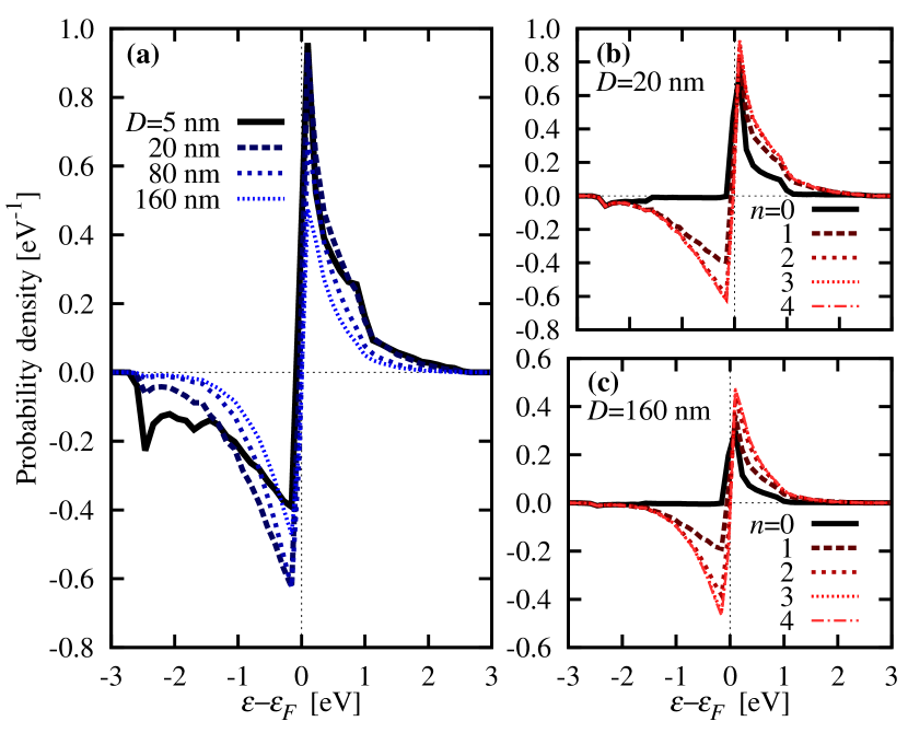
Figure 2: (a) Hot carrier energy distribution reaching the surface of spherical gold nanoparticles of various diameters $D$, normalized to one absorbed photon ($\lambda=490$ nm). This distribution is the perturbation from equilibrium: negative probabilities here correspond to holes. Note increasing thermalization with increasing $D$. (b,c) Cumulative carrier distributions that reach after scattering $\leq n$ times in 20 and 160 nm nanoparticles. Note that holes predominantly reach after 1 scattering event, and the contributions of successive scattering events diminishes rapidly (at a faster rate for smaller particles).

To begin, we examine the carrier distribution in energy and scattering count. Figure 2 shows the collected carrier distributions, both (a) total and (b-c) by scattering event, in spherical gold nanoparticles of various diameters. As expected, the smaller particles collect more carriers at low scattering counts. In addition, even at a given scattering count the smaller particle collects carriers of higher energy than the larger particle, because the mean free path of carriers decreases with increasing energy Brown et al. (2015).

Broadly speaking then there are two primary effects which vary with particle size: the first is a change in regime; small particles collect carriers nearly ballistically, whereas large particles collect them semi-diffusively. The second is a change in energy scale; large particles preferentially collect low-energy carriers as high-energy carriers scatter more readily. Note that small nanoparticles will additionally generate carriers by intraband transitions due to the nanoscale field geometry (Landau damping). However, phonon-assisted transitions dominate over this effect in particles larger than about 40 nm Brown et al. (2015), which is the regime in which transport effects are important anyway. We therefore focus on these larger nanostructures and do not explicitly include geometry-assisted carrier excitations in the results presented below.

Figures 2(b-c) reveal another key feature: the asymmetry between electron and hole scattering. High-energy holes in gold are located in the $d$ bands and have a much smaller mean free path than electrons of comparable energy because of lower band velocities Brown et al. (2015). As a result almost no holes are collected before the first scattering event. Collection then peaks after the first scattering and subsequently diminishes rapidly as the holes thermalize. The implication of this result for hole-driven solid-state and photochemical systems is that structures should be designed either below the high-energy hole mean free path length scale ($\sim 1-3$ nm) to collect them before the first scattering event, or around the intermediate-energy hole mean free path scale ($\sim 10$ nm) to exploit the once-scattered holes.

Finally, Figures 2(b-c) show that with increasing numbers of scattering events, the carrier energy distributions approach symmetric electron and hole perturbation close to the Fermi level, corresponding to an increase of electron temperature as expected. Notice that it takes only 3-4 scattering events to approach this limit, underscoring the importance of designing hot carrier devices in the sub-to-few mean free path scale.

The results discussed above so far assumed perfect collection at the surface. In realistic metal-semiconductor interfaces, injection of carriers from the metal to the semiconductor is possible only when the carrier energy exceeds the Schottky barrier height, and when the carrier momentum tangential to the interface is conserved across it Dalal (1971). This energy and momentum-dependent injection probability limits carrier collection efficiency Leenheer et al. (2014), and is sensitive to the energy-momentum dispersion relations of both the metal and the semiconductor, their energy level alignment at the interface, as well as to the roughness of the interface Chalabi et al. (2014). The NESSE framework contains information regarding the momentum distributions impinging on the surface for each scattering count $n$, and can readily be coupled to a detailed model of the injection probability.

Here, we focus on the effect of carrier injection on carrier transport within the metal, and therefore adopt simplified injection probability models that would introduce the maximum effect on carrier transport. Figure 3 examines the carrier distribution collected at the surface of a gold nanoparticle with varying surface collection properties. We compare four distinct scenarios here, one in which all carriers are collected (ideal) and three in which carriers are only collected above a specific energy. Note that the carriers that are not collected are assumed to reflect back into the material, where they can undergo further scattering processes.

These scenarios suggest that, by and large, fractional reflection of carriers at one energy has the primary effect of reducing carrier collection at that energy. The secondary effect of reintroducing the reflected carriers into the material only minimally enhances collection at other energies. Moreover this enhancement is limited to energies just above the collection threshold, and noticeable only for smaller particles where the reflected carriers are likely to reach another surface prior to additional scattering. This observation has an important implication both for experimental design and hot carrier device simulation: the available hot carrier flux at the surface is mostly independent of the surface collection property, cleanly separating the geometric design of the metal structure with the material design of the metal-collector interface.

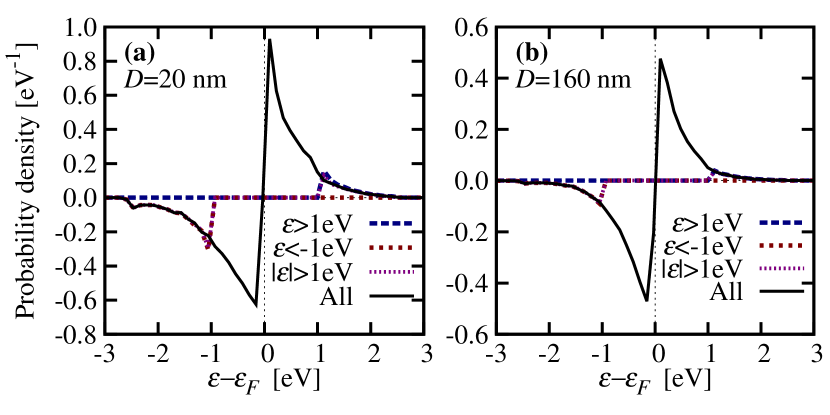
Figure 3: Dependence of hot carrier energy distribution reaching the surface on what carrier energies are allowed to pass through, for particles of diameter (a) 20 nm and (b) 160 nm. When only electrons with $\varepsilon>1$ eV pass through, reflected holes slightly enhance the number of these electrons, and vice versa, when only holes with $\varepsilon<-1$ eV pass through. However this is a small effect, especially for larger dimensions, so it is safe to assume that the carrier distribution reaching the surface is independent of the selection rules for hot carrier extraction at the surface.

Having examined the dependence on energy and scattering properties in spherical particles where spatial variations are less important, we now turn to complex structures with high spatial inhomogeneity and exploit the full power of the NESSE framework. Figure 4 shows carrier distributions resolved in energy and space for a gold bowtie nanoantenna (100 nm equilateral triangles with 40 nm thickness, 10 nm corner radius and a 30 nm gap), illuminated at normal incidence with the electric field direction along the gap and at a resonant wavelength of 650 nm. For this structure and illumination, the field intensity (central top panel), and hence the initial distribution of generated carriers, are sharply localized near the gap. The remaining top panels show the carrier fluxes of holes (left) and electrons (right) above different cutoff energies, normalized per absorbed photon per unit total surface area. Note that these normalized fluxes are dimensionless, but they are not probabilities; they can exceed one both because they are a ratio of carrier flux at one point to the average absorbed photon flux, and because each electron-electron scattering event produces multiple lower energy hot carriers.

The collected carriers localize quite strongly near the field maximum, indicating that field enhancement remains a significant factor even after transport processes are accounted for. Importantly, however, the extent of localization of collected carriers is strongly dependent on the energy of collected carriers. With a higher energy threshold for collection, the overall carrier flux diminishes and becomes more strongly localized towards the high-field gap region. This is also shown in the carrier energy distributions reaching the surface at various distances from the gap region in the bottom panel of Figure 4. Low-energy carriers can reach further from the high-field ‘hot spots’ both because of their higher mean free path and because they can be generated by scattering of higher energy carriers.

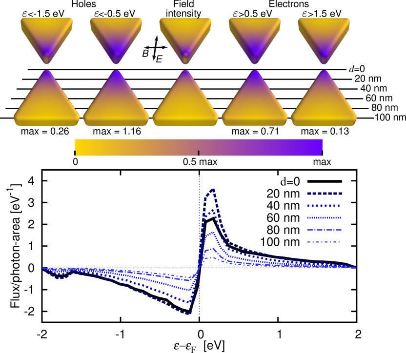
Figure 4: Spatially-resolved hot carrier energy distribution reaching the surface of a gold bowtie nanoantenna illuminated on resonance (650 nm). The top panels compare the spatial distribution of the electric field with fluxes of electrons or holes with energy further than 0.5 or 1.5 eV from the Fermi level, while the lower panels show the average energy-resolved carrier flux in various spatial slices. The fluxes are normalized per absorbed photon per unit area of the surface. Higher energy carriers decay rapidly and are localized to the electromagnetic ‘hot spots’, whereas lower energy carriers can reach further away.

Overall these results show that both the electromagnetic field distribution and the carrier scattering properties play a vital role in shaping the carrier distributions that reach the surface. Predictions solely based on field intensity will overstate carrier localization, particularly at lower energies, while predictions made without accounting for the field distribution will completely miss the spatial inhomogeneity. Experimentally, this spatial inhomogeneity on the tens to hundreds of nanometers is vital to understand hot carrier imaging, photodetection, photovoltaic and photochemical energy conversion, which all involve carrier collection into a semiconductor or molecule.Cortes et al. (2017); Tagliabue et al. (2018) However, optical probes of the carrier response (which we can predict quantitatively using our first-principles framework as shown previously Brown et al. (2017)) cannot sense this inhomogeneity due to the diffraction limit, and instead measure a spatially-averaged result. The hot carrier distribution that we predict here is critical to understand experiments where hot carrier transport matters, precisely because it is not possible to measure these distributions directly.

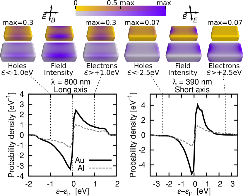
Figure 5: Comparison of spatially- and energy-resolved hot carrier fluxes reaching the surface of a gold (upper) and aluminum (lower) rectangular nanorod illuminated at 800 nm wavelength for the long axis (left) and 390 nm wavelength for the short axis (right). The top panels compare the spatial distributions of carrier flux with energy greater than 1.5eV (left) or 2.5eV (right) away from the Fermi level, while the lower panels show the spatially-averaged energy distributions. Fluxes are normalized per photon absorbed per unit area of the surface. Aluminum is less efficient at collecting low energy carriers due to a shorter electron-phonon scattering mean free path, but enhances high-energy electron collection compared to gold because of increased generation of (and comparable mean free paths for) high-energy electrons.

Finally, we investigate the influence of material choice on the carrier distribution, and in particular, due to the increasing interest in aluminum plasmonics, compare carrier distributions in gold and aluminum structures with similar geometries. In particular, we pick the rectangular nano-antenna geometry shown in Figure 5, with long-axis length 140 nm, short-axis length 80 nm, height 40 nm and 10 nm corner radius. At normal incidence, the resonant absorption frequency depends both on the material and whether the polarization (electric field) direction is along the long or short axis. In particular, we find broad absorption resonances centered at 600 nm and 800 nm respectively for aluminum and gold for the long-axis polarization, and at 390 nm and 610 nm respectively for the short-axis polarization. In order to compare carrier dynamics keeping all other parameters similar, we pick a common long-axis illumination wavelength of 800 nm and a short-axis illumination wavelength of 390 nm, which covers the greatest range of photon energies and exhibits strong absorption in both materials. Since we care about the collected carriers per absorbed photon, minor differences in the absolute absorption cross section are irrelevant.

The top panels of Figure 5 show the spatially-resolved carrier fluxes above a threshold energy in both materials and for both illuminations. As before, the carriers are less localized than the field intensity and the spatial extent increases with decreasing energy due to the higher mean free path and secondary-scattered contributions at lower energies. This effect is comparable in the two materials. Now, compare the probabilities of carrier collection at various energies in the two materials, also shown in the bottom panels as an energy distribution integrated over the structure. At low energies, the carrier collection is overall smaller in aluminum because of a lower electron-phonon mean free path close to the Fermi level (in turn because of lighter atoms and higher density of states in Al) Brown et al. (2015). At higher energies, the mean free path is dominated by electron-electron scattering which is similar between the two materials, and the collection probabilities become comparable. However, at energies above the interband threshold of gold, accessible by the 390 nm short-axis illumination, aluminum exhibits much stronger collection of high-energy electrons compared to gold, because most of the photon energy is now deposited in the $d$-band holes in gold Sundararaman et al. (2014). Aluminum wins for high-energy electrons because of a more favorable initial distribution and comparable carrier transport.

V Conclusions and Outlook

We have presented a new general theoretical and computational framework, NESSE, for transport phenomena far from equilibrium and demonstrated its utility in detail for hot carrier physics in large nanoscale to mesoscale structures. NESSE hybridizes the best features of phase-space (Boltzmann) and particle-based (Monte Carlo) methods and allows us to bridge ab initio electronic structure calculations, carrier collision integrals and electromagnetic simulations to predict the dynamics of photo-excited carriers. The detailed analysis of scattering mechanisms and transport presented here, specialized for the case of plasmonic hot carrier dynamics, provides insight into designing new materials and device motifs which are suitable for carrier transport. Material design is especially relevant for doped-semiconductor plasmonic materials where electronic band structures, and hence phase-space for generation as well as scattering, could be controlled by altering composition. This work additionally paves the way for geometric design of hot carrier devices that carefully optimize against and exploit carrier scattering.

In general, NESSE fills a void in theoretical methods to analyze far-from-equilibrium semi-classical transport phenomena with highly-detailed models of the scattering processes, such as those involving electrons and phonons in the hot carrier example treated in detailed here. It will therefore be invaluable in several areas of physics where transport of charged particles in strong nonequilibrium is pervasive, at length scales both microscopic and astronomical.

References

- Altewischer et al. (2002) E. Altewischer, M. P. van Exter, and J. P. Woerdman, Nature 418, 304 (2002).
- Gramotnev and Bozhevolnyi (2010) D. K. Gramotnev and S. I. Bozhevolnyi, Nat Photon 4, 83 (2010).
- Atwater and Polman (2010) H. A. Atwater and A. Polman, Nat Mater 9, 205 (2010).
- Schuller (2010) J. A. Schuller, Nature Mater. 9, 193 (2010).
- Brongersma et al. (2015) M. L. Brongersma, N. J. Halas, and P. Nordlander, Nat Nano 10, 25 (2015).
- Takahashi and Tatsuma (2011) Y. Takahashi and T. Tatsuma, Applied Physics Letters 99, 182110 (2011).
- Wang and Melosh (2011) F. Wang and N. A. Melosh, Nano Letters, Nano Letters 11, 5426 (2011).
- Jang et al. (2018) Y. J. Jang, K. Chung, J. S. Lee, C. H. Choi, J. W. Lim, and D. H. Kim, ACS Photonics 5, 4711 (2018).
- Hobbs et al. (2017) R. G. Hobbs, W. P. Putnam, A. Fallahi, Y. Yang, F. X. Kärtner, and K. K. Berggren, Nano Letters 17, 6069 (2017).
- Schuck (2013) P. J. Schuck, Nat Nano 8, 799 (2013).
- Adleman et al. (2009) J. Adleman, D. Boyd, D. Goodwin, and D. Psaltis, Nano Lett. 9, 4417 (2009).
- Awazu (2008) K. Awazu, J. Am. Chem. Soc. 130, 1676 (2008).
- Brus (2008) L. Brus, Acc. Chem. Res. 41, 1742 (2008).
- Christopher et al. (2011) P. Christopher, H. Xin, and S. Linic, Nature Chem. 3, 467 (2011).
- Chen et al. (2011) J.-J. Chen, J. C. S. Wu, P. C. Wu, and D. P. Tsai, J. Phys. Chem. C 115, 210 (2011).
- Cushing and Wu (2013) S. K. Cushing and N. Q. Wu, Interface 22, 63 (2013).
- Frischkorn and Wolf (2006) C. Frischkorn and M. Wolf, Chem. Rev. 106, 4207 (2006).
- Wu et al. (2015) K. Wu, J. Chen, J. R. McBride, and T. Lian, Science 349, 632 (2015).
- Inouye et al. (1998) H. Inouye, K. Tanaka, I. Tanahashi, and K. Hirao, Phys. Rev. B 57, 11334 (1998).
- Furube et al. (2007) A. Furube, L. Du, K. Hara, R. Katoh, and M. Tachiya, J. Am. Chem. Soc 129, 14852 (2007).
- Harutyunyan et al. (2015) H. Harutyunyan, A. B. F. Martinson, D. Rosenmann, L. K. Khorashad, L. V. Besteiro, A. O. Govorov, and G. P. Wiederrecht, Nat Nano 10, 770 (2015).
- Knight et al. (2011) M. W. Knight, H. Sobhani, P. Nordlander, and N. J. Halas, Science 332, 702 (2011).
- Zheng et al. (2015) B. Y. Zheng, H. Zhao, A. Manjavacas, M. McClain, P. Nordlander, and N. J. Halas, Nat Commun 6 (2015).
- Buntin et al. (1988) S. Buntin, L. Richter, R. Cavanagh, and D. King, Phys. Rev. Lett. 61, 1321 (1988).
- Ziman (1964) J. M. Ziman, Principles of the Theory of Solids (Cambridge University Press, 1964).
- Chen and Tao (2009) F. Chen and N. J. Tao, Accounts of Chemical Research 42, 429 (2009), pMID: 19253984, http://dx.doi.org/10.1021/ar800199a .
- Del Fatti et al. (2000) N. Del Fatti, C. Voisin, M. Achermann, S. Tzortzakis, D. Christofilos, and F. Vallée, Phys. Rev. B 61, 16956 (2000).
- Tame et al. (2013) M. S. Tame, K. R. McEnery, S. K. Ozdemir, J. Lee, S. A. Maier, and M. S. Kim, Nat Phys 9, 329 (2013).
- Stefanucci and van Leeuwen (2013) G. Stefanucci and R. van Leeuwen, Nonequilibrium Many-Body Theory of Quantum Systems: A Modern Introduction (Cambridge University Press, 2013).
- Thoss and Evers (2018) M. Thoss and F. Evers, J. Chem. Phys. 148, 030901 (2018).
- Perfetto et al. (2015) E. Perfetto, A.-M. Uimonen, R. van Leeuwen, and G. Stefanucci, Phys. Rev. A 92, 033419 (2015).
- Zhou et al. (2018) T. Zhou, P. Zheng, S. C. Pandey, R. Sundararaman, and D. Gall, J. Appl. Phys. 123, 155107 (2018).
- Zhang et al. (2016) Y. Zhang, C. Yam, and G. C. Schatz, J. Phys. Chem. Lett. 7, 1852 (2016).
- Downing et al. (2017a) C. A. Downing, E. Mariani, and G. Weick, Phys. Rev. B 96, 155421 (2017a).
- Downing et al. (2017b) C. A. Downing, E. Mariani, and G. Weick, J. Phys.: Condens. Matter 30, 025301 (2017b).
- Runge and Gross (1984) E. Runge and E. K. U. Gross, Phys. Rev. Lett. 52, 997 (1984).
- Wang et al. (2015) L. Wang, R. Long, and O. V. Prezhdo, Ann. Rev. Phys. Chem. 66, 549 (2015).
- (38) K. Stephan, Adv. Energy Mater. 7, 1700440.
- Stefanucci and Almbladh (2004) G. Stefanucci and C.-O. Almbladh, Europhys. Lett. 67, 14 (2004).
- Long and Prezhdo (2014) R. Long and O. V. Prezhdo, J. Am. Chem. Soc. 136, 4343 (2014).
- Wang et al. (2016) H. Wang, J. Bang, Y. Sun, L. Liang, D. West, V. Meunier, and S. Zhang, Nature Commun. 7, 11504 (2016).
- Manjavacas et al. (2014) A. Manjavacas, J. G. Liu, V. Kulkarni, and P. Nordlander, ACS Nano 8, 7630 (2014).
- Ma et al. (2015) J. Ma, Z. Wang, and L.-W. Wang, Nature Commun. 6, 10107 (2015).
- Golovchenko (1976) J. A. Golovchenko, Phys. Rev. B 13, 4672 (1976).
- Hagelaar and Pitchford (2005) G. J. M. Hagelaar and L. C. Pitchford, Plasma Sources Science and Technology 14, 722 (2005).
- Guyer and Krumhansl (1966) R. A. Guyer and J. A. Krumhansl, Phys. Rev. 148, 766 (1966).
- Chen (2001) G. Chen, Phys. Rev. Lett. 86, 2297 (2001).
- Mermin (1970) N. D. Mermin, Phys. Rev. B 1, 2362 (1970).
- Binder (1986) K. Binder, Monte Carlo Methods in Statistical Physics (Springer, 1986).
- Sundararaman et al. (2014) R. Sundararaman, P. Narang, A. S. Jermyn, W. A. Goddard, and H. A. Atwater, Nat. Commun. 5 (2014), 10.1038/ncomms6788.
- Brown et al. (2015) A. M. Brown, R. Sundararaman, P. Narang, W. A. Goddard, and H. A. Atwater, ACS Nano (2015), 10.1021/acsnano.5b06199, pMID: 26654729, http://dx.doi.org/10.1021/acsnano.5b06199 .
- Brown et al. (2016) A. M. Brown, R. Sundararaman, P. Narang, W. A. Goddard, and H. A. Atwater, Phys. Rev. B 94, 075120 (2016).
- Brown et al. (2017) A. M. Brown, R. Sundararaman, P. Narang, A. M. Schwartzberg, W. A. Goddard, and H. A. Atwater, Phys. Rev. Lett. 118, 087401 (2017).
- Cortes et al. (2017) E. Cortes, W. Xie, J. Cambiasso, A. Jermyn, R. Sundararaman, P. Narang, S. Schlucker, and S. A. Maier, Nature Commun. 8, 14880 (2017).
- Tagliabue et al. (2018) G. Tagliabue, A. Jermyn, R. Sundararaman, A. Welch, J. DuChene, R. Pala, A. Davoyan, P. Narang, and H. Atwater, Nature Commun. 9, 3394 (2018).
- Narang et al. (2017) P. Narang, L. Zhao, S. Claybrook, and R. Sundararaman, Advanced Optical Materials in press, 1600914 (2017).
- Rangel et al. (2012) T. Rangel, D. Kecik, P. E. Trevisanutto, G.-M. Rignanese, H. Van Swygenhoven, and V. Olevano, Phys. Rev. B 86, 125125 (2012).
- Hedin and Lundqvist (1970) L. Hedin and S. Lundqvist, J. Phys. C: Solid State Phys. 23, 1 (1970).
- Sundararaman et al. (2017) R. Sundararaman, K. Letchworth-Weaver, K. Schwarz, D. Gunceler, Y. Ozhabes, and T. A. Arias, SoftwareX 6, 278 (2017).
- Dalal (1971) V. L. Dalal, J. Appl. Phys. 42, 2274 (1971).
- Leenheer et al. (2014) A. J. Leenheer, P. Narang, N. S. Lewis, and H. A. Atwater, J. Appl. Phys. 115, 134301 (2014).
- Chalabi et al. (2014) H. Chalabi, D. Schoen, and M. L. Brongersma, Nano Lett. 14, 1374 (2014).