An explanation of remarkable emission line profiles in post-flare coronal rain

Abstract

We study broad red-shifted emission in chromospheric and transition region lines that appears to correspond to a form of post-flare coronal rain. Profiles of Mg II, C II and Si IV lines were obtained using the IRIS instrument before, during and after the X2.1 flare of 11 March 2015 (SOL2015-03-11T16:22). We analyze the profiles of the five transitions of Mg II (the $3p-3s$ $h$ and $k$ transitions, and three lines belonging to the $3d-3p$ transitions). We use analytical methods to understand the unusual profiles, together with higher resolution observational data of similar phenomena observed by Jing et al. (2016). The peculiar line ratios indicate anisotropic emission from the strands which have cross-strand line center optical depths ($k$-line) of between 1 and 10. The lines are broadened by unresolved Alfvénic motions whose energy exceeds the radiation losses in the Mg II lines by an order of magnitude. The decay of the line widths is accompanied by a decay in the brightness, suggesting a causal connection. If the plasma is $\mathrel{\hbox to0.0pt{\lower 3.7pt\hbox{$\sim$} \hss}\raise 1.7pt\hbox{$<$}}99$% ionized, ion-neutral collisions can account for the dissipation, otherwise a of dynamical process seems necessary. Our work implies that the motions are initiated during the impulsive phase, to be dissipated as radiation over a period of an hour, predominantly by strong chromospheric lines. The coronal “rain” we observe is far more turbulent that most earlier reports have indicated, with implications for plasma heating mechanisms.

1. Introduction

The purpose of the present paper is to analyze some curiously broad, red-shifted profiles of emission lines obtained with the Interface Region Imaging Spectrograph instrument (IRIS: De Pontieu et al., 2014) a few minutes after the impulsive phase of a flare. The X2.1 flare of 11 March 2015 (SOL2015-03-11T16:22) occurred in the active region (AR) NOAA 12297 and was accompanied by a filament eruption. Detectable hard X-Ray emission observed with Reuven Ramaty High Energy Solar Spectroscopic Imager (RHESSI: Lin et al., 2002) began near 16:16 UT, reached a peak at 16:21 UT and returned to its near-quiescent state near 16:35 UT. The broad, redshifted emission of interest here started abruptly near 16:26 UT.

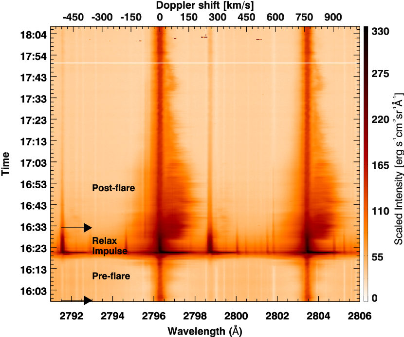
Figure 1.— Cubic root scaled intensity profiles of the Mg II $h$ and $k$ lines (for the first slit position, at y=-175”) are shown as a function of wavelength and time. Doppler shift values with respect to the k-line position are also included. The two profiles shown in Figure 2 are from 15:57:51 and 16:32:31 UT, indicated by arrows.

Typical profiles of the Mg II $h$ and $k$ (at air wavelengths 2802.7 Å and 2795.5 Å, respectively) lines during this phase are shown in Figures 1 and 2. These profiles appear to differ qualitatively from all earlier theoretical and most observational studies on coronal rain, the emission lines being unusually broad.

By themselves, these data admit several possibilities of interpretation. Fortuitously, some partly resolved “fine structure” with similar spectral properties has been observed in another solar flare (Jing et al., 2016). Their work focused on observations of spectral lines with $0\farcs 03$ sampling, through narrow-band filters. Although not discussed by them, Figure 7b in their paper also shows Mg II spectral data from IRIS during the post-flare stage that, without doubt, arise from the same phenomenon we analyze here. Thus, the broad, red-shifted emission features of Figures 1 and 2 are coincident with the onset of a return of emitting plasma along post-flare loops (see Figures 7c and 7d of Jing et al., 2016). These phenomena shown by Jing et al. (2016) and in the present work are unquestionably a form of coronal rain.

Usually seen as plasma emission in chromospheric and transition region lines (partially ionized or neutral plasma), or as absorption in EUV images, coronal rain forms as a consequence of instability in coronal loops. In non-flaring active region loops, thermal instability leads to catastrophic cooling (Cally & Robb, 1991). Numerous observations and models have studied coronal rain (Kohutova & Verwichte, 2016; Moschou et al., 2015, and references within), finding typical redshifts of $\sim$80 km s^-1. These authors have highlighted multi-stranded and multi-thermal structure, but without reference to broad line widths. Plasma condensation after eruptive flares can produce similar phenomena (Song et al., 2016), although the physical processes may differ. Kleint et al. (2014) have found bursty flows associated with bright-points at the edge of the sunspot umbra, that show a striking similarity to the profiles analyzed here, but lasting only $\sim$20 s.

Here we study the Mg II and other lines from IRIS to try to constrain the physical nature of the unusually broad lines associated with raining plasma. The various observed parameters, when judiciously combined with the results of Jing et al. (2016), constrain the nature of the raining plasma and its origins more tightly than has been achieved in the past. The primary lines of interest here are listed in Table 1.

Table 1Atomic transitions of interest

Ion	$\lambda$ Å	upper level	lower level	gf	$\Upsilon(T_{\mathrm{e}})$
Mg II	2802.705	$3p~{}^{2}{\rm P}^{o}_{\mathrm{1/2}}$	$3s~{}^{2}{\rm S}_{\mathrm{1/2}}$	0.64	5.6
	2795.528	$3p~{}^{2}{\rm P}^{o}_{\mathrm{3/2}}$	$3s~{}^{2}{\rm S}_{\mathrm{1/2}}$	1.3	12.3
	2790.777	$3d~{}^{2}{\rm D}_{\mathrm{3/2}}$	$3p~{}^{2}{\rm P}^{o}_{\mathrm{1/2}}$	1.9	9.1
	2797.930	$3d~{}^{2}{\rm D}_{\mathrm{3/2}}$	$3p~{}^{2}{\rm P}^{o}_{\mathrm{3/2}}$	0.39	4.8
	2797.998	$3d~{}^{2}{\rm D}_{\mathrm{5/2}}$	$3p~{}^{2}{\rm P}^{o}_{\mathrm{3/2}}$	3.5	18.3
	…	$3d~{}^{2}{\rm D}_{\mathrm{5/2}}$	$3p~{}^{2}{\rm P}^{o}_{\mathrm{1/2}}$	…	2.5
	…	$3d~{}^{2}{\rm D}_{\mathrm{3/2}}$	$3s~{}^{2}{\rm S}_{\mathrm{1/2}}$	…	1.2
	…	$3d~{}^{2}{\rm D}_{\mathrm{5/2}}$	$3s~{}^{2}{\rm S}_{\mathrm{1/2}}$	…	1.8
C II	1334.5323	$2s^{2}2p~{}^{2}{\rm D}_{\mathrm{3/2}}$	$2s^{2}2p~{}^{2}{\rm P}^{o}_{\mathrm{1/2}}$	0.26	1.4
	1335.6625	$2s^{2}2p~{}^{2}{\rm D}_{\mathrm{3/2}}$	$2s^{2}2p~{}^{2}{\rm P}^{o}_{\mathrm{3/2}}$	0.051	0.9
	1335.7077	$2s^{2}2p~{}^{2}{\rm D}_{\mathrm{5/2}}$	$2s^{2}2p~{}^{2}{\rm P}^{o}_{\mathrm{3/2}}$	0.46	2.9
	…	$2s^{2}2p~{}^{2}{\rm D}_{\mathrm{5/2}}$	$2s^{2}2p~{}^{2}{\rm P}^{o}_{\mathrm{1/2}}$	…	0.5
Si IV	1402.77	$3p~{}^{2}{\rm P}^{o}_{\mathrm{1/2}}$	$3s~{}^{2}{\rm P}_{\mathrm{1/2}}$	0.54	7.3

Data are from the NIST spectroscopic database (Kramida et al., 2015), wavelengths above 2000 Å are in air, otherwise they are in vacuum. Collisional data are from Sigut & Pradhan (1995); Blum & Pradhan (1992); Zhang et al. (1990). The Maxwellian-averaged collision strengths $\Upsilon(T_{\mathrm{e}})$ are given for $T_{\mathrm{e}}=10^{4}$ K for the singly charged ions, and at $T=10^{5}$ K for Si IV.

Being a consequence of the unknown mechanisms by which mass and energy are transported into the solar corona, there are many outstanding questions concerning coronal rain. Here we focus upon extracting as much information from the IRIS data to study the origins of the cool material arising from the flare, and its remarkable thermal structure. Post-flare chromospheric spectra have been obtained for decades in lines such as H$\alpha$. The Mg II data analyzed here have advantages over H$\alpha$. The line emissivities and opacities are more simply related to thermal properties of the emitting plasma (discussed below).

We study five Mg II lines (two of which are blended), collectively they are sensitive to different thermal conditions. Thus, we can perform a simple quantitative analysis of the data with minimal assumptions. Our work complements much recent work (e.g. Antolin et al., 2015; Jing et al., 2016) which studies broad- or narrow-band imaging, by analyzing the behavior of line profiles. These profiles differ so dramatically from those previously modeled using existing numerical methods, that we adopt analytical methods. Our work should later inspire further numerical simulations, such as that of Fang et al. (2013), which might attempt to better understand the origin of the enormous linewidths spanning over 300  km s^-1, pointing to energetic magnetic waves or (less likely) turbulence as the culprit.

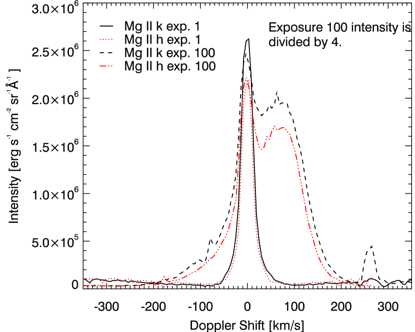
Figure 2.— Typical intensity profiles of the Mg II $h$ and $k$ lines are shown as a function of Doppler shift, positions indicated by arrows in Figure 1. Two profiles shown are those of 15:57:51 UT (exp. 1), from the pre-flare phase, and those of 16:32:31 UT (exp. 100), from the post-flare phase. The very broad profiles seen during the 16:32:31 UT image are the focus of the present work.

2. Observations

On 11 March 2015, the IRIS instrument acquired data of AR NOAA 12297 during a flare watch campaign. Data were downlinked from nine spectral windows. Here we analyze those containing the lines of Mg II, C II and Si IV, together with data obtained by the Atmospheric Imaging Assembly (AIA: Lemen et al., 2012) and Helioseismic and Magnetic Imager (HMI: Schou et al., 2012) instruments on the Solar Dynamics Observatory spacecraft (SDO: Pesnell et al., 2012). The IRIS slit was moved sequentially and repeatedly to four positions offset by 0, 2, 4, 6$\arcsec$ in the E-W direction on the solar surface. A total of 1230 such pointings were acquired. We focus on data from exposures 110 to 490. At each slit position, spectral data with exposures of 4 seconds was acquired. To complete one cycle of 4 slit positions took $\approx 21$ seconds. During the flare, the exposure times were decreased for the FUV wavelengths by an automatic flare-triggered mechanism, to prevent over-exposure, without affecting the total raster duration. The projected slit is 0.33$\arcsec$ wide. The spatial and spectral samplings were 0.33$\arcsec$/pixel and 0.05092 Å/pixel for the NUV region. For the FUV regions the spectral sampling was $0.02544$ Å/pixel (FUV2) and $0.02596$ Å/pixel (FUV1).

We applied iris_orbitvar_corr_l2s.pro, a routine in the IRIS SolarSoft package, to correct for spacecraft orbital variations. Following the procedure in Liu et al. (2015), we then obtained wavelength-integrated emission-line intensities in physical units (see Table 2), which refer to the obvious components in emission above the photospheric absorption line and continua. For comparison we include the values for a quiet sun (QS) patch outside the active region along those from a representative position within the peculiar spectrum region at different time instances. These values are the sum over both line core and extended red-shifted profile, including multiple lines where is the case. All velocities are determined relative to the average quiet Sun spectrum.

IRIS slit-jaw images (SJI) at 1330, 1400 and 2832 Å were also acquired during the raster steps 0, 3, and 1 respectively. Each SJI set had a temporal sampling of 20.76 seconds on average, and spatial sampling of 0.33$\arcsec$/pixel, spanning a total field of view (FOV) of $126\arcsec\times 119\arcsec$. Four such images are shown in Figure 3.

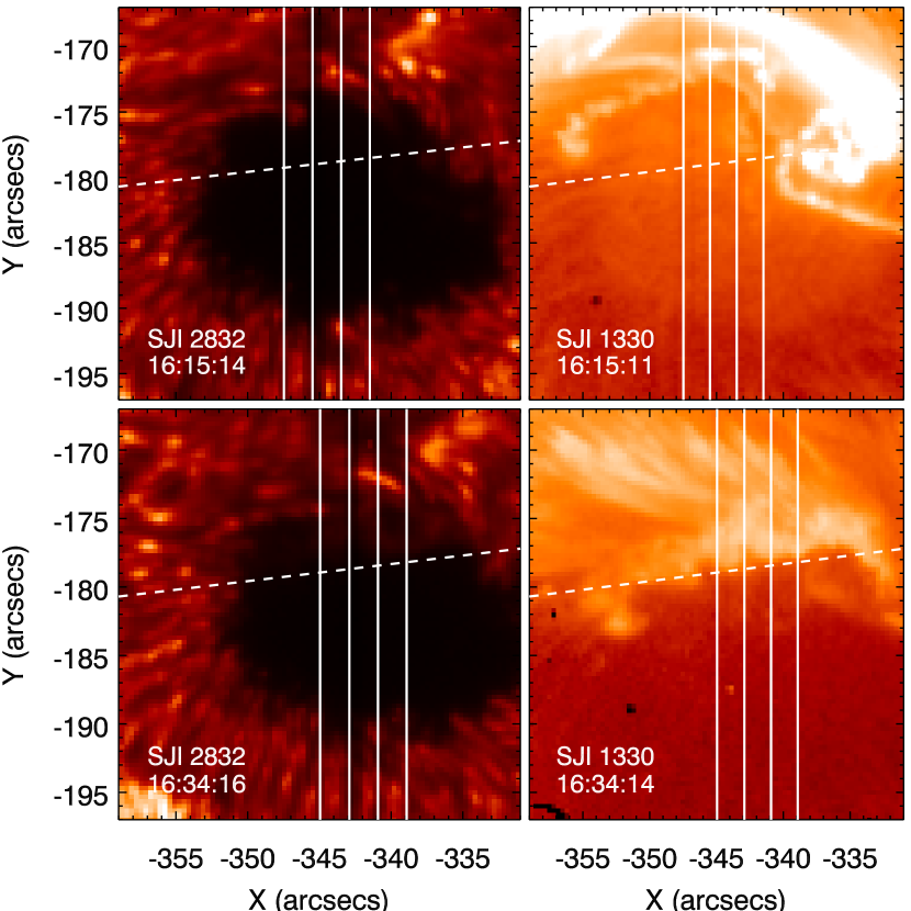
Figure 3.— IRIS SJI images in the 2832 channel (left) and the 1330 channel (right), before and after the impulsive phase. A logarithmic scaling has been applied to SJI 1330. The vertical lines are the positions of the IRIS slits and the oblique dashed line is the lower boundary (in the N-S direction) of the peculiar spectra. Plasma flows can be seen above this dashed line in the SJI 1330 post-flare images.

The flare appears to have been triggered by the accelerated rise of a filament starting near 16:13 UT. Flare emissions started at 16:16 UT, the flaring reaching the emission maxima at 16:20 UT. This maximum high energy flare emission, as observed by RHESSI, was located at (X,Y)=(-354,-171)$\arcsec$, a region not covered by the spectral slit positions.

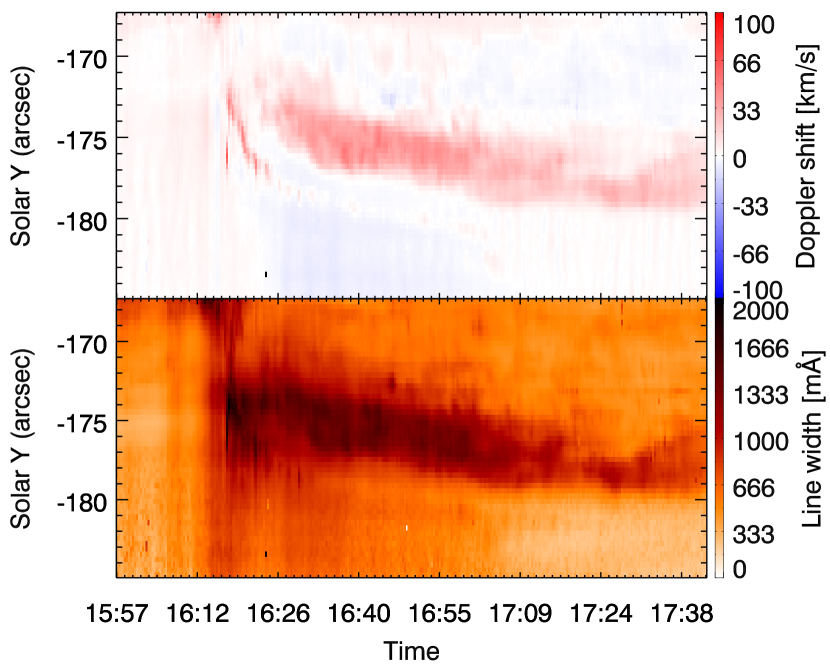
Figure 4.— Doppler shift (top) and line widths (bottom) maps for the Mg II k-line, showing the time evolution of the extended redshifted emission for the first slit position. The peculiar emission sweeps the same region as the flare ribbon. Positive Doppler shift values refer to red shift and negative values to blue shift.

We examine the evolution of the spectra at different locations along the flare ribbon. We found locations of extended very broad and redshifted emission at the same locations swept over by the evolving and propagating flare ribbon, lasting for more than an hour after the flaring event. To highlight typical Doppler shifts and line widths, in Figure 4 we show the first velocity-weighted moment (Doppler shift) and second moment (line width) of the Mg II k-line, normalized to the zeroth moment. The Figure shows data only for the first slit position. In passing, we note that the smaller amplitude blue-shifts in the umbra probably correspond to umbral flashes, studied for example by Bard & Carlsson (2010).

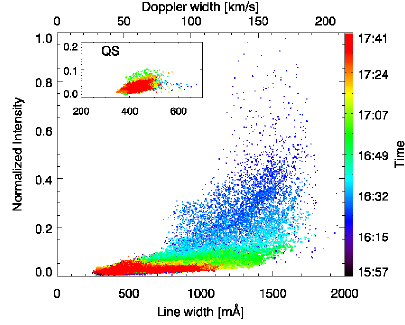
Figure 5.— Normalized Intensity vs line width correlation for all the pixels between -170$\arcsec$ and -180$\arcsec$. The color represents the time of the observation and the insert represents the data from a QS patch outside the active region.

To highlight the evolution of the line width over the whole region of interest, we represented the normalized intensity of the profile as a function of the line width in Figure 5, along with an insert of the same dependence for a quiet sun patch outside the active region. The color represents the time of the exposure, with early times being masked by later emission. The QS distribution is centered around 400 mÅ and shows little scatter. The distribution for the peculiar emission region is centered around 500 mÅ before the flare and it shows an increase in both intensity and line width after the flare. The intensity decreases in time to pre-flare values, while the width still has an extended tail up to about 1100 mÅ suggesting that the raining phenomenon is still ongoing.

Figure 6 shows the position of the four IRIS slits projected onto an image constructed from data from the SDO/HMI instrument. The HMI data are the standard reductions of the “720s” product, including vector magnetic field data. The field azimuth in the plane perpendicular to the line of sight (LOS) has not been disambiguated. Note that the four slit positions extend across the entire sunspot centered near (X,Y)=(-340,-182)$\arcsec$. The broadened profiles are found above the penumbra, they are marked as the solid components of the dashed lines shown in the figure. The lengths and positions of these lines correspond to the average locations where the anomalously broad profiles occur. These regions are quite separate from the magnetic neutral line. Instead, they lie above regions of modest LOS field, large perpendicular field, whose direction follows parallel or anti-parallel to the axis of a “dark intrusion” (Fig. 6) centered at (X,Y)=(-343,-176)$\arcsec$, a location of where systematic upward-directed photospheric motions of $\approx$1–1.5 km s^-1 are present (but not shown here).

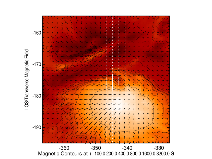
Figure 6.— Vector magnetic field parameters at 16:24 UT. The vertical dashed lines show the positions of the IRIS slit, the solid portion of which approximately shows the extent of very broad lines seen in the Mg II $h$ and $k$ lines shown in previous figures.

Intensity profiles of the Mg II $h$ and $k$ lines are shown in Figure 2. Representative data of interest here are from exposure number 100 in our sample obtained at 16:32:31 UT. In the figure these are shown as dashed lines. The time dependence of these profiles is shown in Figure 1. The IRIS instrument’s compensation for the Sun’s average rotation was used, so that the images show the changing conditions over approximately the same areas of the Sun.

For convenience, in Figure 1, we identify four episodes in the evolution of the Mg II: A pre-flare phase (before 16:20 UT); An impulsive phase (16:21 UT); A relaxation phase (16:21 to 16:27 UT) ; A post-flare (PF) phase (16:25 UT to beyond 17:00 UT). The PF phase is the subject of the present paper. These phases are self-evident in the data. The relaxation phase is simply the transient response of the line profiles to the sudden release of energy in the impulsive phase, judging by the time scale of the decay which seems appropriate. The chromosphere has a thickness of $\approx 1500$ km, and pressure perturbations (shocks) will propagate a little above the sound speed of $\approx 7-10$  km s^-1. A few sound crossing times corresponds to about 5 minutes. The relaxation phase is most clearly seen in the narrow $3d-3p$ lines of Mg II, close to 2791 and 2798 Å in this figure. The $h$ and $k$ resonance lines of Mg II are at 2796.3 and 2803.5 Å.

Table 2Observed frequency-integrated emission-line intensity (erg cm^-2 s^-1 sr^-1)

Multiplet	Mg II	Mg II	C II	Si IV
	$h+k$	$3d-3p$	1334	1403
Phase			+1335
QS	$5.36\times 10^{5}$	…	$6070$	$572$
Pre-flare	$1.83\times 10^{6}$	…	$5.16\times 10^{4}$	2840
Impulse	$4.36\times 10^{7}$	$\approx 1.36\times 10^{7}$	$1.73\times 10^{7}$	$>3.86\times 10^{6}$
Relax	$2.77\times 10^{7}$	$4.81\times 10^{6}$	$4.39\times 10^{6}$	$3.51\times 10^{5}$
Post-flare	$\mathbf{1.82\times 10^{7}}$	$\mathbf{\approx 4.51\times 10^{5}}$	$\mathbf{1.45\times 10^{6}}$	$\mathbf{2.04\times 10^{5}}$

Quiet Sun data are from the darkest regions along the IRIS slit. We used calibration factors returned by iris_get_response.pro: dn2phot_sg = 4.0 (FUV) and 18.0(NUV), and effective areas of 0.474, 1.042 and 0.23 cm² for the 1335, 1400 and 2800 Å wavelengths, respectively. The intensities in boldface will be used throughout this article.

Profiles of C II resonance lines near 1335 Å show similar spectral line shapes to $h$ and $k$, as does the 1403 Å line of Si IV. Both lines are slightly broader (in Doppler units) than the $h$ and $k$ lines. However, the duration of the broad PF profiles in both cases are appreciably shorter. The intensities of these lines are also 10-100$\times$ smaller than $h$ and $k$ (Table 2).

3. Analysis

3.1. Summary of observed properties

We focus only on the “postflare” (PF) phase, since these profiles are as yet unexplained. The spatio-temporal behavior of the broad PF profiles appears to be unrelated to other phases (see Figure 1). They are most simply interpreted as simple (unreversed) emission superposed onto the more“normal” profile represented by exposure 1 shown in Figure 2. During the PF phase the $h$ and $k$ profiles have several salient features: (1) the total intensities of the broad profiles are larger than the core intensities, and the time variations vary largely independently of the core intensities; (2) the PF $h$ and $k$ intensities are remarkably smooth across the line profile at each time of observation, but they change a little between exposures; (3) the intensities are in the ratio $k/h$ = 1.15 across almost the entire line profiles (see Fig. 2); (4) the lines are far broader than the net redshift; (5) the PF emission patches are $\approx 4-5$ Mm across; (6) in both the $h$ and $k$ lines the bright PF profiles begin abruptly 6-7 minutes after the impulsive phase (see Figure 1 and 4); (7) the broad components are not obviously self-reversed; (8) the profiles are very similar across all regions sampled by the spectrometer’s slit.

It is interesting to relate these profiles to the other lines. The PF $3d-3p$ transitions are far weaker than during the impulsive and relaxation phases, compared with the $h$ and $k$ lines ($3p-3s)$. To the above points we add (9), namely that the $h$ and $k$ lines, and those of Si IV and C II all have widths in Doppler units of about $w=100$  km s^-1, and their centroids are red-shifted by about +60  km s^-1 (see Figures 4 and 5).

Point (1) implies that PF profiles are not caused by scattering of bright photons from the core. Regarding point (3), optically thin conditions produce ratios of intensities of 2:1. Hence the PF plasmas are optically thick in the $h$ and $k$ lines. Remarkably, the same is true for the 1334/1335 C II lines whose intensities are close to 1:1, compared to the optically thin ratio of 1:2. Point (2) suggests that the unresolved motions are physically much smaller than resolvable scales. Points (4) and (8) suggest that, if opacity broadening is negligible, there is more energy in unresolved motions (widths) than in resolved motions (shifts). Photon scattering can, however, both broaden and shift the lines, this will be discussed below. The intensities of the various lines at various phases are listed in Table 2.

3.2. A reference model

We examine the PF profiles using parameters in a reference model of the emitting plasma. We will assume that the plasma exists in strands with a width W$\approx 100$ km (Jing et al., 2016), that has number densities of hydrogen nuclei close to $10^{12}$ particles per cm³, and that these particles are all at temperatures of $\approx 10^{4}$ K. If $T_{\mathrm{e}}$ exceeds $2-3\times 10^{4}$ K, Mg becomes doubly ionized. The justification for the adopted density is weak. It exceeds that at the very top of the pre-flare chromosphere by an order of magnitude, but flare models propel mass from deeper layers of the chromosphere higher into the corona, on time scales of a minute or less for M and X class events. (e.g. Abbett & Hawley, 1999; Allred et al., 2005). In an X-class flare (with $\approx 10^{11}$ erg cm^-2 s^-1 of energy flux directed towards the chromosphere), the mass per unit of ejected material is expected to be about $m=10^{-2}F_{\mathrm{11}}$ g cm^-2, estimated from the last panels of Figures 3 and 5 of Allred et al. (2005). Here $F_{\mathrm{11}}$ is the downward-directed energy flux in units of 10¹¹ erg cm^-2 s^-1. If this mass is spread uniformly along a tube of constant area with length $L$, then the number density on average is $\approx m/\mu m_{\mathrm{H}}L$, where $\mu=1.36$ is the mean atomic weight of the largely neutral pre-flare plasma and $m_{\mathrm{H}}$ is the mass of the hydrogen atom. With $L=10^{9}L_{\mathrm{10}}$ cm and with $L_{\mathrm{10}}$ corresponding to $10$ Mm, we have:

$$n_{\mathrm{H}}\approx 5\times 10^{12}L^{-1}_{\mathrm{10}}F_{\mathrm{11}}\ \ {\rm cm^{-3}}$$ (1)

This provides a crude justification for our adopted estimate of $n_{\mathrm{H}}=10^{12}$ cm^-3 for the raining plasma after this X2 class flare . We use variables normalized to the average values: $W=10^{7}W_{\mathrm{100}}$ cm, $n=10^{12}n_{\mathrm{12}}$ cm^-3, and $T=10^{4}T_{\mathrm{e4}}$ K. We will also assume that the unresolved “microturbulent” velocities are of order $\xi=10\xi_{\mathrm{10}}$  km s^-1, with $\xi_{\mathrm{10}}=1$, which is of order the sound speed at $T_{\mathrm{4}}=1$. In this reference model, $W_{\mathrm{100}}=n_{\mathrm{12}}=T_{\mathrm{e4}}=\xi_{\mathrm{10}}$=1. Note that the observed line widths are $w=\xi=100$  km s^-1, ten times broader than the reference width, for reasons to be discussed below.

The model is used below to explore conditions under which these lines might form, understanding that the chosen values are educated guesses.

3.3. Radiative transfer

We consider the formation of the Mg II lines in a structure that consists of an array of strands that comprise an episode of coronal rain. Thus we look first at the spectrum emitted by one elemental strand of width $W_{\mathrm{100}}=1$.

3.3.1 Strand optical depths

Two observations imply that the optical depth of the $k$ line across the emitting stands is $\mathrel{\hbox to0.0pt{\lower 3.7pt\hbox{$\sim$} \hss}\raise 1.7pt\hbox{$>$}}$ 1, at line center. Firstly, the emission is self-excited within the raining plasma itself, i.e. there is no identifiable dominant external source of irradiation. Secondly, the $k$/$h$ line ratios are far from the optically thin ratio of 2:1 (Figure 2).

With an absorption oscillator strength $f$, the transition between levels 1 and 2 has an opacity at line center (in units of cm^-1) of (e.g. Mihalas, 1978)

$$\kappa_{\mathrm{0}}=\frac{\pi e^{2}}{m_{\mathrm{e}}c}n_{\mathrm{1}}f/\Delta\nu\ =\ 0.0264\ n_{\mathrm{1}}f/\Delta\nu,$$ (2)

where $m_{\mathrm{e}}$ is the electron mass, $e$ is the elementary charge, $n_{\mathrm{1}}$ is the number density of Mg II ions in the lower level, and $\Delta\nu$ is the Doppler width of the line in Hz. Then, the optical depth across a strand of width $W$ whose axis has an angle $\vartheta$ with the line-of-sight is given by:

$$\tau_{\mathrm{0}}=0.0264\ \frac{n_{\mathrm{1}}fW}{\mu\,\Delta\nu},\ \ \mu=\cos\vartheta.$$ (3)

Let us assume that most Mg atoms in the strands are in the ground state of Mg II, then, with a logarithmic abundance of Mg of 7.42 relative to hydrogen (Allen, 1973), we have $n_{\mathrm{1}}=n_{\mathrm{H}}\times 10^{7.42-12}=3\times 10^{6}n_{\mathrm{12}}$ cm^-3. With a Doppler width $\xi$ of 10 km s^-1, $\Delta\nu\approx 3.6\times 10^{10}\xi_{\mathrm{10}}$ Hz, and for $k$, $f=0.6$, then

$$\kappa_{\mathrm{0}}=1.1\times 10^{-5}n_{\mathrm{12}}/\xi_{\mathrm{10}}\ \ {\rm cm^{-1}}$$ (4)

With $W_{\mathrm{100}}=W/100~{}{\rm km}$ we have

$$\tau_{\mathrm{0}}=110\frac{n_{\mathrm{12}}}{\xi_{\mathrm{10}}}\frac{W_{\mathrm{100}}}{\mu}.$$ (5)

In this reference model the $h$ and $k$ lines have $\tau_{\mathrm{0}}\approx 10^{2}$ across the strands.

The observation that the $k:h$ ratio in the PF profile is 1.15, far from the thin ratio of 2:1, has two possible explanations. The first is that the lines might be effectively thick, a condition that is true for the Mg II $h$ and $k$ lines formed in the stratified chromosphere (e.g. Linsky & Ayres, 1978) causing the Sun’s $k/h$ ratio from various non-flaring regions on the Sun to be close to 1.1-1.5 (e.g. Kerr et al., 2015). The second possibility is that the radiation emerging from the strands is anisotropic, and that the $h$ and $k$ lines have different anisotropy under conditions of modest optical depth.

The latter case seems far more likely, as can be seen by comparing the escape probability of line photons from the strand core with the destruction probability. In Appendix A we show that the absorption of Mg II photons by background continuum is negligible in the reference model. The probability of destruction by collisions from the $k$ line can be evaluated simply as

$$\varepsilon=\frac{C_{\mathrm{31}}}{A_{\mathrm{31}}+C_{\mathrm{31}}}$$ (6)

where $C_{\mathrm{31}}$ is the collision rate from level 3 to level 1, the dominant collision rate out of the line’s upper level (level 3). and $A_{\mathrm{31}}$ is the Einstein coefficient for spontaneous radiative emission (Allen, 1973). Using parameters from Table 1 we find $A_{\mathrm{31}}=2.7\times 10^{8}$ sec^-1, and $C_{\mathrm{31}}\approx 4\times 10^{4}n_{\mathrm{e12}}T_{\mathrm{e4}}^{-1/2}$ sec^-1. Here we must use the electron density $n_{\mathrm{e12}}$ because electrons are responsible for the bulk of the collisions.

$$\varepsilon\approx\frac{C_{\mathrm{31}}}{A_{\mathrm{31}}+C_{\mathrm{31}}}\approx 10^{-4}n_{\mathrm{e12}}/\sqrt{T_{\mathrm{e4}}}.$$ (7)

A reasonable approximation for $P_{\mathrm{esc}}$ for resonance lines is

$$P_{\mathrm{esc}}\approx\frac{1-\exp(-\tau_{\mathrm{0}})}{\tau_{\mathrm{0}}}$$ (8)

(e.g. Frisch, 1984), so that in the reference model for the $k$ line, using equation (5) then

$$P_{\mathrm{esc}}/\varepsilon\approx\frac{10^{2}\xi_{\mathrm{10}}\mu\sqrt{T_{\mathrm{e4}}}}{n_{\mathrm{e12}}n_{\mathrm{12}}W_{\mathrm{100}}}.$$ (9)

It seems $P_{\mathrm{esc}}\gg\varepsilon$ for reasonable physical parameters.

Together with the observation that the broad profiles are not self-reversed, we conclude that the lines are effectively thin in the coronal rain.

3.3.2 $k:h$ ratio and radiation anisotropy

How can radiation anisotropy explain the line ratios in the rain phenomenon? The lines of $h$ and $k$ differ in opacity by a factor of two. We can imagine a simple case of cylindrical strands where the optical depth of $h$ is $\approx 1/2$, and that of $k$ is $\approx 1$. The $h$ line photons can escape directly from deeper within the strand than the $k$ line photons. In essence, the $h$ line will radiate more isotropically from the core of the strand, whereas $k$ photons will scatter preferentially into the path of shortest escape, i.e. perpendicularly to the main axis of the strand. The observed line ratio will change from $2:1$ even if the total emission into all directions is in the ratio 2:1. We would expect $k:h>2:1$ perpendicular to the strand’s main axis of symmetry, and $k:h<2:1$ in other directions.

If the optical depths are substantially higher ($\tau_{\mathrm{0}}(k)\approx 10$, say), then the differential effect is reduced to the outermost cylinders comprising the strand (assuming it is a cylinder, cf. Lipartito et al., 2014), the radiation being more isotropic in the opaque deeper core of the strand.

We conclude that we are seeing the strands at a slant angle far from $90^{\circ}$ and $0^{\circ}$ to the strand’s main axis, and that $\tau_{\mathrm{0}}$ should be $>1$ but less than $\approx 10$ in the $k$ line, in these strands. The value of 110 computed from our reference calculation lies close to the necessary optical depth, when we note that the nearest boundary of the strand for escape is at a distance of at most $W/2$ not $W$, and, as we will argue below, $\xi_{\mathrm{10}}$ is an underestimate, thus the core photons will see a boundary $\mathrel{\hbox to0.0pt{\lower 3.7pt\hbox{$\sim$} \hss}\raise 1.7pt\hbox{$<$}}$ 110/2 optical depths distant.

Related to this problem is the effect of atomic polarization when scattering dominates the source function ($\varepsilon\ll 1$). The $J=1/2$ upper level of $h$ is not polarizable, and the scattered intensity of the $J=1/2\rightarrow J=1/2$ transition ($h$ line) is isotropic. However, the polarizable $J=3/2$ upper level’s atomic polarization can change the observed intensity ratios under conditions of anisotropy even by the “diffuse” photons self-generated within the cylinder (Landi Degl’Innocenti & Landolfi, 2004). We estimated these effects to be small, on the order of a few percent using calculations similar to those applied to He I lines by Judge et al. (2015).

3.4. Frequency-integrated intensities

If a line is effectively thin across an emitting strand, the emission is simply the sum of the emission along the line-of-sight. To an accuracy of a factor of two, we can ignore the anisotropy, and we find, for the $k$ line:

$$I_{\mathrm{thin}}\approx\frac{h\nu_{\mathrm{31}}}{4\pi}{n_{\mathrm{1}}C_{\mathrm{13}}}\frac{W}{\mu}\ \ {\rm erg~{}cm^{-2}~{}s^{-1}sr^{-1}}.$$ (10)

where $C_{\mathrm{13}}$ is the collisional excitation rate (Gabriel & Jordan, 1971; Burgess & Tully, 1992). Within a factor of 2 or so, we can set $\mu=0.5$, and this expression gives, multiplying by two for the sum of the two lines:

$$I_{\mathrm{thin}} \approx \frac{h\nu_{\mathrm{31}}}{4\pi}{n_{\mathrm{1}}C_{\mathrm{13}}}\frac{W}{\mu}$$ (11)

$$\approx 1.4\times 10^{6}n_{\mathrm{12}}n_{\mathrm{e12}}\exp\left(4.86(1-\frac{1}{T_{\mathrm{e4}}})\right)W_{\mathrm{100}}$$

for our reference calculation. The observed intensities for both lines are of the order of $1.6\times 10^{7}$ erg cm^-2 s^-1 sr^-1. With $T_{\mathrm{e4}}=2$ we find $I_{\mathrm{thin}}\approx 1.1\times 10^{7}$ erg cm^-2 s^-1 sr^-1. We regard this as reasonable agreement with our adopted reference calculation, noting that the calculation depends exponentially on $T_{\mathrm{e4}}$ and on the product $n_{\mathrm{12}}n_{\mathrm{e12}}$, and allowing for the possibility that there is more than one such strand of emission along each line of sight observed by IRIS.

3.5. Doppler widths and shifts

The Doppler shifts of 50-60  km s^-1 are compatible with the acceleration of cool plasma elements due to gravity under free fall from a few Mm above the surface. But more interesting constraints come from the observed linewidths. We work in units of the Doppler broadening parameter, $\xi$. The observed lines are $\approx 10\times$ broader than our reference model can produce. Particle densities are far below those needed for significant collisional broadening. An optical depth of $10$ at the center of the $k$ line would produce photon emission up to about $\xi_{\mathrm{10}}\sqrt{\ln\tau_{\mathrm{0}}}\approx 1.5\xi_{\mathrm{10}}$ from line center, assuming complete redistribution and using an argument due to Osterbrock (1962).

It seems highly unlikely that photon scattering at high optical depths is the source of the broad line emission. The lack of a clear self-reversal near the cores of the PF broad profiles appears to suggest also that photon scattering is not a major contributor PF profile widths. We are forced to conclude that the lines are formed under conditions of modest optical depth ($\tau_{\mathrm{0}}(k)\mathrel{\hbox to0.0pt{\lower 3.7pt\hbox{$\sim$} \hss}\raise 1.7pt\hbox{$<$}}10$), but in which the radiation is anisotropic.

Given our modest estimates of optical depth, the broad emission widths are some $15-20\times$ the sound speed where Mg II emission usually forms ($T_{\mathrm{e}}\mathrel{\hbox to0.0pt{\lower 3.7pt\hbox{$\sim$} \hss}\raise 1.7pt\hbox{$<$}}2\times 10^{4}$ K). Under these extreme conditions it is likely that shocks would quickly dissipate such small-scale motions, if they were purely hydrodynamic and small-scale. Thus, magnetic fields are responsible for the unresolved motions.

3.6. Mg II $h$ and $k$ and the $3d-3p$ transitions

Unlike the $3p-3s$ transitions, the $3d-3p$ transitions, when in emission, are certainly not optically thick within the strands. The lower ($3p$) levels have a population of $\mathrel{\hbox to0.0pt{\lower 3.7pt\hbox{$\sim$} \hss}\raise 1.7pt\hbox{$<$}}\exp(-4.86/T_{\mathrm{e4}})$ times the $3s$ lower level of the $h$ and $k$ lines, thus the $3d-3p$ optical depths are orders of magnitude smaller than $h$ and $k$. The observed intensity ratios (the blend of the 2797.930 and 2797.998 Å lines, relative to the 2790.930 Å line) are indeed close to the optically thin ratios of 2:1.

The $3d-3p$ transitions differ from $h$ and $k$ in another essential way. Electron excitation to the $3d$ levels from the $3s$ ground level is optically forbidden. The cross sections are dominated by core penetration of the Mg$+$ ion by the incoming electrons. There is no long-range interaction. When the $3p$ level populations are far below Boltzmann relative to $3s$, as is the case when the lines are effectively thin (photon escape in $h$ and $k$ reducing the $3p$ populations), collisional excitation of the $3d$ levels occurs predominantly only from the $3s$ level. Then, again ignoring anisotropies in the radiation field,

$$\frac{I_{\mathrm{3d-3p}}}{I_{\mathrm{3p-3s}}}\approx\frac{C_{\mathrm{3s-3d}}}{C_{\mathrm{3s-3p}}}$$ (12)

which becomes

$$\frac{I_{\mathrm{3d-3p}}}{I_{\mathrm{3p-3s}}}\approx\frac{\Upsilon_{\mathrm{3s-3d}}}{\Upsilon_{\mathrm{3s-3p}}}\exp\left(-\frac{4.86}{T_{\mathrm{e4}}}\right)\approx\frac{1}{6}\exp\left(-\frac{4.86}{T_{\mathrm{e4}}}\right)$$ (13)

Inserting the observed ratio $\approx 1/40$ into equation (13), we find $T_{\mathrm{e4}}\approx 2.5$, or $\approx 2.0$ allowing for the radiation anisotropy in the $k$ line.

We note that the work of Pereira et al. (2015) forces the formation of the $3d-3p$ transitions into the dense, lower chromosphere, through their choice of model atmosphere. In their model, the $h$ and $k$ lines are thermalized where the $3d-3p$ transitions form, and so the $3d$ levels are populated largely through the two allowed transitions $3s-3p$ followed by $3p-3d$.

3.7. Dielectronic recombination

The process of dielectronic recombination (DR) can lead to emission on the red side of resonance lines (e.g. Gabriel & Jordan, 1971). In the case of Mg II, $3pnl$ states can form as intermediate states in a Mg${}^{+}3s$ + e^- collision, a process called dielectronic capture. If the intermediate states decay radiatively to $3snl$ states emitting a $3p-3s$ photon, called a “stabilizing transition”, the process is a dielectronic recombination. For singly charged ions, DR rates are typically some $10^{2-3}$ times smaller than the direct rate for collisional excitation. For Mg${}^{+}-e^{-}$ DR the results of Altun et al. (2006) yield a total rate of about 0.003 of the direct rate. Therefore, if the broad PF profiles were caused by a superposition of DR then their intensities would be some $10^{2-3}$ times smaller than that of the core emission. This is not observed (Figures 1 and 2).

3.8. Sudden onset of post-flare coronal rain emission.

Inspection of Figure 1 shows that the PF profiles begin abruptly near 16:26 UT. They show a two-fold rise in intensity across all wavelengths that takes between 2 and 3 time steps, say $t=40$ seconds. Fast changes are also seen throughout the PF phase in Figure 1, but with smaller amplitudes.

These data are difficult to reconcile if we assume that the linewidths of the emitting plasmas arise from a mixture of LOS velocities on macroscopic scales. At a given slit position, various plasma elements would arrive at different times as they each follow their own trajectory. Let us suppose that plasma is ejected into the corona from one or both flare footpoints. On their way to crossing the slit, they acquire various LOS velocities as a result of the (unknown) dynamics in the post-flare tubes of magnetic flux. Depending on the trajectories, if one assumes that the PF line profiles are superpositions of macroscopic flows, then the elements will cross the slit with a broad distribution of arrival times. This is contrary to the observations. The short rise time $t\approx 40$ seconds across the entire profile imply that, if caused by different arrival times, the plasma elements would have to coordinate themselves such that 50  km s^-1 upward moving plasma would “know” when to cross the slit as well as the 150  km s^-1 downward moving plasma. Simply put, there would have to be a linear relationship between velocity and projected distance $d$ from the slit,

$$v\cos\vartheta=d\cos\vartheta/t.$$ (14)

It does not make sense that the Sun would know about the special position of the IRIS slit in such a fashion.

What then is the cause of the two-fold rise in intensity across all wavelengths within $t=40$ seconds? We can conceive of two explanations: (1) The rain plasma has small-scale motions (with a magnitude of $\approx 100$  km s^-1) within a coherent large-scale flow, making $\xi_{\mathrm{10}}\approx 10$, or (2) The plasma is indeed moving at a variety of macrosopic velocities, but that there is a special thermodynamic process making the plasma visible on a time scale of $40$ seconds.

The second explanation can be discounted because the the history of each plasma element determines whether lines of a certain element will become visible at a certain time. For example, if the raining plasma is unheated and is at densities close to 10¹¹ cm^-3, the cooling time is of order 100 seconds (Anderson & Athay, 1989). At 100  km s^-1 the plasma can travel $\approx 9$ Mm before it cools significantly. Again, we are faced with the untenable position that the IRIS slit would have to be a “special” place on the Sun for this explanation to hold water, each element evolving along its own trajectory. A change in opacity is discounted because we know of no mechanism to suddenly reveal only the PF broad profiles at 16:26 UT.

Thus we are left with the first explanation which is similar to real rain on Earth.

3.9. Origins of the broad lines

The large value of $\xi\approx 100$  km s^-1 is still consistent with the required optical depths to make the radiation differentially anisotropic between $h$ and $k$, because for $k$ we find a reduction in $\tau_{\mathrm{0}}$ from $13$ to $1.3$, owing to the denominator of equation (2). We are then left to explain why the line width speeds are so high, and the fact that the line shifts are about half those of the widths. The red-shifts correspond to plasma dropped in free fall from a height of $\approx 5$ Mm. It seems that gravity at least can account for such red-shifts, even if it is superposed onto more energetic small-scale dynamics. The red-shifts will therefore concern us no more.

The field strength needed to achieve an Alfvén speed of 100  km s^-1 when $n_{\mathrm{12}}=1$ is merely $\approx 17$ G. This is two orders of magnitude smaller than the photospheric fields that lie below the raining plasma region, which have $B\mathrel{\hbox to0.0pt{\lower 3.7pt\hbox{$\sim$} \hss}\raise 1.7pt\hbox{$>$}}1500$ G (Figure 6). So it appears that Alfvén waves generated after the impulsive phase can easily carry enough kinetic energy to account for the broad lines, if otherwise undamped, for some tens of minutes after the impulsive phase. The kinetic energy density of the unresolved motions with $n_{\mathrm{12}}=1$ is $\rho\xi^{2}\approx$23 erg cm^-3. If these persist along a length $L_{\mathrm{10}}=1$ of a strand, then these motions amount to an energy density per unit area of about $2\times 10^{10}$ erg cm^-2. A large X-class flare releases some $10^{11}$ erg cm^-2 s^-1 during the impulsive phase, for some $10^{2-3}$ seconds, giving an available energy density per unit area of $10^{13-14}$ erg cm^-2. It therefore seems reasonable that 1 part in 10³ of this impulse might reside in residual wave motions in the post-flare magnetic fields, and become evident in the widths of the lines observed with IRIS reported here. Also, the strands occupy a small volume of the magnetic structures in which they exist (Jing et al., 2016), therefore considerably more magnetic energy might feed into the strands from neighbouring plasma not revealed in the Mg II or other UV emission lines.

Can MHD (Magneto-Hydro-Dynamic) oscillations live for a period of an hour or so during which the broad Mg II lines decay? To answer this question would require MHD simulations across multiple scales, since the dissipation of magnetic energy requires the (non-linear) generation of small physical scales. A recent physical discussion of various incomplete calculations done to date shows that it may take a very long time to dissipate wave energy in loops containing small-scale density inhomogeneities (Cargill et al., 2016), calling into question the viability at least of phase mixing to describe coronal heating. Below we consider other explanations.

4. Discussion

We have examined all salient features of the peculiar IRIS post-flare line profiles of Mg II, C II and Si IV, with accompanying slit-jaw and magnetic data. By elimination we are led, remarkably, to a consistent picture in which unresolved Alfvénic motions – waves or turbulence – are generated and gradually decay over a period of more than one hour. The decay of the magnetic energy is about an order of magnitude larger than the radiation losses from the strong Mg II lines, suggesting a causal connection between them. The peculiar line ratios and profiles are consistent with strands of plasma of width 100 km, and they require an optical depth across them of between $1$ and $10$ in the $k$ line.

If we apply the observed intensities and ratios to equations to (13) and (11) to solve for model parameters, we have $T_{\mathrm{e}}\approx 2\times 10^{4}$ K, and $n^{2}_{\mathrm{12}}W_{\mathrm{100}}\approx 0.4$. Assuming $W_{\mathrm{100}}=1$ then $n_{\mathrm{12}}\approx 0.6$. But this analysis does not acknowledge that because of the evidence of unresolved motions there is certainly a distribution of plasma with temperature, and that lines such as the Mg II $3d-3p$ and C II 1335 form in hotter plasma than $h$ and $k$. Given the exponential dependence of radiative losses on temperature, we therefore suspect, but cannot prove, that for $h$ and $k$ a smaller value of $T_{\mathrm{e}}$ is appropriate. If this is the case then $n_{\mathrm{12}}>0.6$. Below we will adopt $n_{\mathrm{12}}=1$ for the sake of argument.

The total flux radiated during the coronal rain phenomenon seen in $h$ and $k$ is $\approx\pi It_{\mathrm{r}}=5\times 10^{7}\times 600\approx 3\times 10^{10}$ erg cm^-2. Here we have used a relaxation lifetime of 10 minutes appropriate for the first part of the relaxation phase where these line intensities were measured (Figure 1). The total radiation losses from chromospheric plasma (due to losses in calcium, iron, hydrogen,..) are between $4\times$ and $10\times$ larger, with larger values occurring at lower plasma temperatures (Anderson & Athay, 1989, Fig. 4). We adopt a value of $4\times$ the $h$ and $k$ losses, to arrive at a total time-integrated radiative flux of $10^{11}$ erg cm^-2.

Above, we found $\rho\xi^{2}L\approx 2.3\times 10^{10}n_{\mathrm{12}}L_{\mathrm{10}}$ erg cm^-2. These rough estimates are within a factor of 4 of one another, so with With $n_{\mathrm{12}}L_{\mathrm{10}}=4$ we have agreement. Perhaps more noteworthy, Figure 1 shows that as the broad line intensities decrease, so does the power in the fluctuations (linewidths). It appears that the Alfvénic fluctuations excited during the impulsive phase, might decay ultimately into radiation via a process that slowly (compared with dynamical time scales $\approx L/V_{\mathrm{A}}$) converts the wave into thermal energy.

Various dynamical mechanisms might achieve this on time scales of an hour, such as phase mixing, resonant absorption (e.g. Narain & Ulmschneider, 1990, 1996), although detailed fully dynamical numerical simulations need to be performed to address the very long damping times suggested by Cargill et al. (2016). Gas-kinetic processes can also efficiently damp oscillations when neutral H or He are abundant in the raining plasma. Ion-neutral collisions would efficiently damp out high frequency wave energy on time scales of the ion-neutral collision time, $\tau_{\mathrm{ni}}\approx 0.4n_{\mathrm{n11}}/\sqrt{T}$ seconds, where $n_{\mathrm{n11}}$ is the ambient neutral density in units of 10¹¹ particles cm^-3 (eq. 16, Holzer et al., 1983). At wave frequencies $\omega$ below the inverse of the collision time, equation 17 of Holzer et al. (1983) applies, which gives time scales of

$$2/(\tau_{\mathrm{ni}}\omega^{2}),\ \ \omega\tau_{\mathrm{ni}}\ll 1.$$ (15)

For example, a three-minute period Alfvén wave has $\omega\approx 1/50$ rad sec^-1, $\omega\tau_{\mathrm{ni}}\approx 10^{-4}$ and then the damping time becomes $20/n_{\mathrm{n11}}$ seconds. If the plasma were 1% neutral then the observed decay time of a few thousand seconds would be naturally explained without needing to invoke dynamical MHD processes.

Lastly, the IRIS profiles resemble those seen in flares of very active stars (Linsky et al., 1989). It is likely our solar analysis can help better understand such enormous flares.

Appendix A Background opacities near 2800 Å

For absorption in the background continuum with opacity $\kappa_{\mathrm{C}}$, effectively thick conditions prevail when

$$P_{\mathrm{esc}}<\kappa_{\mathrm{C}}/\kappa_{\mathrm{0}}.$$ (A1)

At 2800 Å, the dominant source of continuous opacity within the strands is probably the Balmer continuum of hydrogen. This can be computed approximately assuming that the $n=2$ levels of hydrogen are populated not too far from LTE relative to the proton density $n_{\mathrm{p}}$, because the radiation temperature in the Balmer continuum ($\approx 6000$K) and electron temperature are within a factor of two or so. Then

$$\kappa_{\mathrm{C}}=n_{\mathrm{2}}\sigma\approx\frac{n^{*}_{\mathrm{2}}}{n^{*}_{\mathrm{p}}}n_{\mathrm{p}}\sigma$$ (A2)

Let $n_{\mathrm{e}}$ be the electron density in cm^-3, $T_{\mathrm{e}}$ the electron temperature in K. Then with (Mihalas, 1978)

$$\frac{n^{*}_{\mathrm{2}}}{n^{*}_{\mathrm{p}}}=2.07\times 10^{-16}n_{\mathrm{e}}\frac{g_{\mathrm{2}}}{g_{\mathrm{p}}}T_{\mathrm{e}}^{-3/2}\exp\left(\frac{I_{\mathrm{2}}}{kT_{\mathrm{e}}}\right),$$ (A3)

using $I_{\mathrm{2}}=3.399$ eV, and using scaled values $n_{\mathrm{e12}}=n_{\mathrm{e}}/10^{12}$ cm^-3, $T_{\mathrm{e4}}=T_{\mathrm{e}}/10^{4}$ K, and with $\sigma\approx 10^{-17}$ cm² (Allen, 1973), then

$$\kappa_{\mathrm{C}}\approx 1.7\times 10^{-14}n_{\mathrm{e12}}T_{\mathrm{e4}}^{-3/2}\ \exp\left(3.945/T_{\mathrm{e4}}\right)n_{\mathrm{p12}}$$ (A4)

Then we find, further assuming $n_{\mathrm{p}}\approx n_{\mathrm{e}}$, and dropping subscripts p,e for convenience,

$$\kappa_{\mathrm{C}}/\kappa_{\mathrm{0}}\approx 2.5\times 10^{-9}n_{\mathrm{12}}\exp\left(3.945/T_{\mathrm{4}}\right)\xi_{\mathrm{10}}/T_{\mathrm{4}}^{3/2}$$ (A5)

Given equation  (5), this ratio would need to be $\approx 0.01$ for the line to be effectively thick due to background continuum absorption. If we set extreme conditions (photosphere-like) of $n_{\mathrm{12}}\approx 10^{1}$, $T_{\mathrm{4}}\approx 0.5$, we can obtain a ratio of $7\times 10^{-5}$.

Therefore we can safely ignore continuum absorption at 2800 Å in the coronal rain.

References

- Abbett & Hawley (1999) Abbett, W. P., & Hawley, S. L. 1999, ApJ, 521, 906
- Allen (1973) Allen, C. W. 1973, Astrophysical quantities (Athlone Press, Univ. London)
- Allred et al. (2005) Allred, J. C., Hawley, S. L., Abbett, W. P., & Carlsson, M. 2005, ApJ, 630, 573
- Altun et al. (2006) Altun, Z., Yumak, A., Badnell, N. R., Loch, S. D., & Pindzola, M. S. 2006, A&A, 447, 1165
- Anderson & Athay (1989) Anderson, L. S., & Athay, R. G. 1989, ApJ, 336, 1089
- Antolin et al. (2015) Antolin, P., Vissers, G., Pereira, T. M. D., Rouppe van der Voort, L., & Scullion, E. 2015, ApJ, 806, 81
- Bard & Carlsson (2010) Bard, S., & Carlsson, M. 2010, ApJ, 722, 888
- Blum & Pradhan (1992) Blum, R. D., & Pradhan, A. K. 1992, ApJS, 80, 425
- Burgess & Tully (1992) Burgess, A., & Tully, J. A. 1992, A&A, 254, 436
- Cally & Robb (1991) Cally, P. S., & Robb, T. D. 1991, 372, 329
- Cargill et al. (2016) Cargill, P. J., De Moortel, I., & Kiddie, G. 2016, ApJ, 823, 31
- De Pontieu et al. (2014) De Pontieu, B., Title, A. M., Lemen, J. R., et al. 2014, Sol. Phys., 289, 2733
- Fang et al. (2013) Fang, X., Xia, C., & Keppens, R. 2013, ApJ, 771, L29
- Frisch (1984) Frisch, H. 1984, Methods in Radiative Transfer, ed. W. Kalkofen (Cambridge Univ.)
- Gabriel & Jordan (1971) Gabriel, A. H., & Jordan, C. 1971, Case Studies in Atomic Collision Physics, Chapt. 4, ed. M. McDowell & E. McDaniel (North-Holland), 209–291
- Holzer et al. (1983) Holzer, T. E., Fla, T., & Leer, E. 1983, ApJ, 275, 808
- Jing et al. (2016) Jing, J., Xu, Y., Cao, W., et al. 2016, Nat.: Scientific Reports, 6
- Judge et al. (2015) Judge, P. G., Kleint, L., & Sainz Dalda, A. 2015, ApJ, 814, 100
- Kerr et al. (2015) Kerr, G. S., Simões, P. J. A., Qiu, J., & Fletcher, L. 2015, A&A, 582, A50
- Kleint et al. (2014) Kleint, L., Antolin, P., Tian, H., et al. 2014, ApJ, 789, L42
- Kohutova & Verwichte (2016) Kohutova, P., & Verwichte, E. 2016, ApJ, 827, 39
- Kramida et al. (2015) Kramida, A., Ralchenko, Y., Reader, J., & NIST ASD Team. 2015, NIST Atomic Spectra Database (version 5.3), [Online]. Available: http://physics.nist.gov/asd. National Institute of Standards and Technology, Gaithersburg, MD., ,
- Landi Degl’Innocenti & Landolfi (2004) Landi Degl’Innocenti, E., & Landolfi, M. 2004, Polarization in Spectral Lines, Vol. 307 of Astrophysics and Space Science Library
- Lemen et al. (2012) Lemen, J. R., Title, A. M., Akin, D. J., et al. 2012, Sol. Phys., 275, 17
- Lin et al. (2002) Lin, R. P., Dennis, B. R., Hurford, G. J., et al. 2002, Sol. Phys., 210, 3
- Linsky & Ayres (1978) Linsky, J. L., & Ayres, T. R. 1978, ApJ, 220, 619
- Linsky et al. (1989) Linsky, J. L., Neff, J. E., Brown, A., et al. 1989, A&A, 211, 173
- Lipartito et al. (2014) Lipartito, I., Judge, P. G., Reardon, K., & Cauzzi, G. 2014, ApJ, 785, 109
- Liu et al. (2015) Liu, W., Heinzel, P., Kleint, L., & Kašparová, J. 2015, Sol. Phys., 290, 3525
- Mihalas (1978) Mihalas, D. 1978, Stellar atmospheres, 2nd Edition., ed. W. H. Freeman & Co. (San Francisco)
- Moschou et al. (2015) Moschou, S. P., Keppens, R., Xia, C., & Fang, X. 2015, Advances in Space Research, 56, 2738
- Narain & Ulmschneider (1990) Narain, U., & Ulmschneider, P. 1990, Space Sci. Rev., 54, 377
- Narain & Ulmschneider (1996) —. 1996, Space Sci. Rev., 75, 453
- Osterbrock (1962) Osterbrock, D. E. 1962, ApJ, 135, 195
- Pereira et al. (2015) Pereira, T. M. D., Carlsson, M., De Pontieu, B., & Hansteen, V. 2015, ApJ, 806, 14
- Pesnell et al. (2012) Pesnell, W. D., Thompson, B. J., & Chamberlin, P. C. 2012, Sol. Phys., 275, 3
- Schou et al. (2012) Schou, J., Scherrer, P. H., Bush, R. I., et al. 2012, Sol. Phys., 275, 229
- Sigut & Pradhan (1995) Sigut, T. A. A., & Pradhan, A. K. 1995, Journal of Physics B Atomic Molecular Physics, 28, 4879
- Song et al. (2016) Song, Q., Wang, J.-S., Feng, X., & Zhang, X. 2016, ApJ, 821, 83
- Zhang et al. (1990) Zhang, H. L., Sampson, D. H., & Fontes, C. J. 1990, Atomic Data and Nuclear Data Tables, 44, 31