On the fine structure splitting of the ${\rm{3p^{4}3d}\,{{}^{4}}{D^{\phantom{o}}_{\mathrm{5/2}}}}$ and ${\rm{3p^{4}3d}\,{{}^{4}}{D^{\phantom{e}}_{\mathrm{7/2}}}}$ levels of Fe X

Abstract

We study UV spectra obtained with the SO82-B slit spectrograph on board SKYLAB to estimate the fine structure splitting of the Cl-like ${\rm{3p^{4}3d}\,{{}^{4}}{D^{\phantom{o}}_{\mathrm{5/2}}}}$ and ${\rm{3p^{4}3d}\,{{}^{4}}{D^{\phantom{e}}_{\mathrm{7/2}}}}$ levels of Fe X. The splitting is of interest because the Zeeman effect mixes these levels, producing a “magnetically induced transition” (MIT) from ${\rm{3p^{4}3d}\,{{}^{4}}{D^{\phantom{e}}_{\mathrm{7/2}}}}$ to ${\rm{3p^{5}}\,{{}^{2}}{P^{{o}}_{\mathrm{3/2}}}}$ for modest magnetic field strengths characteristic of the active solar corona. We estimate the splitting using the Ritz combination formula applied to two lines in the UV region of the spectrum close to 1603.2 Å, which decay from the level ${\rm{3p^{4}(^{1}D)3d}\,{{}^{2}}{G^{\phantom{e}}_{\mathrm{7/2}}}}$ to these two lower levels. The MIT and accompanying spin-forbidden transition lie near 257 Å. By careful inspection of a deep exposure obtained with the S082B instrument we derive a splitting of $\mathrel{\hbox to0.0pt{\lower 3.7pt\hbox{$\sim$} \hss}\raise 1.7pt\hbox{$<$}}7\pm 3$ cm^-1. The upper limit arises because of a degeneracy between the effects of non-thermal line broadening and fine-structure splitting for small values of the latter parameter. Although the data were recorded on photographic film, we solved for optimal values of line width and splitting of $8.3\pm 0.9$ and $3.6\pm 2.7$ cm^-1.

1. Introduction

Grumer et al. (2014) and Li et al. (2015, 2016) have presented a novel method by which mixing of atomic states by the Zeeman effect can in principle be used to determine magnetic field strengths in the solar corona. The method is readily illustrated by non-degenerate first order quantum perturbation theory. Given a “pure” set of atomic states $|\alpha_{\mathrm{i}}J_{\mathrm{i}}\rangle$ with angular momentum quantum numbers $J_{\mathrm{i}}$ and other quantum numbers $\alpha_{\mathrm{i}}$, the Zeeman effect will mix the states to first order by addition of the magnetic Hamiltonian $H_{\mathrm{M}}=\mu_{\mathrm{i}}B$ where $B$ is the field induction and $\mu_{\mathrm{i}}$ the magnetic moment of state $i$, such that

$$|\alpha_{\mathrm{j}}J_{\mathrm{j}}\rangle\approx\sum_{\mathrm{i}}d_{\mathrm{i}}|\alpha_{\mathrm{i}}J_{\mathrm{i}}\rangle$$ (1)

where the values of mixing coefficients $d_{\mathrm{i}},i\neq j$ are proportional to $H_{\mathrm{M}}$ and inversely proportional to the unperturbed fine structure (FS) splitting $E_{\mathrm{j}}-E_{\mathrm{i}}$ (e.g. Li et al., 2015, eq. 3).

The spectrum of Fe X is bright in the Sun’s corona, the well known “coronal red line” at 6376.29 Å (${\rm{3p^{5}}\,{{}^{2}}{P^{{o}}_{\mathrm{1/2}}}}$ to ${\rm{3p^{5}}\,{{}^{2}}{P^{{o}}_{\mathrm{3/2}}}}$) is one of the strongest forbidden transitions visible during eclipse or with coronagraphs (Kiepenheuer, 1953; Billings, 1966). Some particular Fe X transitions in the EUV, which can be seen clearly against the dim EUV solar disk, have been shown to be of special interest for the challenging problem of measuring the coronal magnetic field (Li et al., 2015). This is because a near level-crossing occurs close to Fe⁹⁺ in the Cl-like iso-electronic sequence, for the two levels ${\rm{3p^{4}3d}\,{{}^{4}}{D^{\phantom{o}}_{\mathrm{5/2}}}}$ and ${\rm{3p^{4}3d}\,{{}^{4}}{D^{\phantom{e}}_{\mathrm{7/2}}}}$. Then $E_{\mathrm{j}}-E_{\mathrm{i}}$ becomes small enough that one mixing coefficient $d_{\mathrm{i}}$ become large enough to produce “magnetically induced transitions” (MITs) that are otherwise forbidden. In Fe X this occurs between the unperturbed levels ${\rm{3p^{4}3d}\,{{}^{4}}{D^{\phantom{e}}_{\mathrm{7/2}}}}$ and ${\rm{3p^{5}}\,{{}^{2}}{P^{{o}}_{\mathrm{3/2}}}}$. The radiative decays of the two levels ${\rm{3p^{4}3d}\,{{}^{4}}{D^{\phantom{o}}_{\mathrm{5/2}}}}$ and ${\rm{3p^{4}3d}\,{{}^{4}}{D^{\phantom{e}}_{\mathrm{7/2}}}}$ thereby become sensitive to the magnetic field in the emitting plasma, which can therefore be measured simply through the ratios of the two line intensities.

For this method to be of practical use, the energy difference $E_{\mathrm{j}}-E_{\mathrm{i}}$ must be known with sufficient accuracy (Li et al., 2016). The latter authors estimated the value of $E_{\mathrm{j}}-E_{\mathrm{i}}$ for levels ${\rm{3p^{4}3d}\,{{}^{4}}{D^{\phantom{o}}_{\mathrm{5/2}}}}$ and ${\rm{3p^{4}3d}\,{{}^{4}}{D^{\phantom{e}}_{\mathrm{7/2}}}}$ using a known magnetic field and the observed intensity ratio. At present, the splitting is believed to be on the order of 3.5 cm^-1 from the Shanghai EBIT measurement, by measurement of the EUV spectrum with a known magnetic field (Li et al., 2016). But given the high sensitivity of the derived magnetic field to the zero-field splitting, it is important to try to constrain the energy splitting through other techniques.

The purpose of the present paper is simply to determine $E_{\mathrm{j}}-E_{\mathrm{i}}$ independently using the Ritz combination principle applied to some forbidden transitions observed during the SKYLAB era using the S082B slit spectrograph. Figure 1 shows a partial term diagram showing the levels of interest to the present work. This diagram is based upon atomic data listed in Table 1.

Figure 1.— A partial term diagram of Fe X showing the levels and (main) transitions of interest. We make measurements of differential wavelengths in the two 1603 Å transitions. From these data we determine the relative energy of the lower (${\rm{}^{4}D}$) levels with an accuracy far greater than in the EUV transitions.

2. Observations and Analysis

The S082B spectrograph provided data from a $2\arcsec\times 60\arcsec$ projected slit with a spectral resolution of 0.06 Å (Bartoe et al., 1977). We searched the logs of the S082B instrument for deep exposures obtained above the solar limb, in the short wavelength channel (970 to 1970 Å). The need for deep, off-limb data is apparent when we consider the low expected intensities of the lines decaying from the ${\rm{3p^{4}(^{1}D)3d}\,{{}^{2}}{G^{\phantom{e}}_{\mathrm{7/2}}}}$ level to the ${\rm{3p^{4}3d}\,{{}^{4}}{D^{\phantom{o}}_{\mathrm{5/2}}}}$ and ${\rm{3p^{4}3d}\,{{}^{4}}{D^{\phantom{e}}_{\mathrm{7/2}}}}$ levels for two reasons. First, the transitions lie close to 1603.2 Å, where the solar continuum seen on the disk is bright. Second, the $L$ and $J$ quantum numbers of the upper level ${\rm{3p^{4}(^{1}D)3d}\,{{}^{2}}{G^{\phantom{e}}_{\mathrm{7/2}}}}$ differs by three and at least 2 from ${\rm{3p^{5}}\,{{}^{2}}{P^{{o}}_{\mathrm{3/2}}}}$ and ${\rm{3p^{5}}\,{{}^{2}}{P^{{o}}_{\mathrm{1/2}}}}$. Collisional excitations to ${\rm{3p^{4}(^{1}D)3d}\,{{}^{2}}{G^{\phantom{e}}_{\mathrm{7/2}}}}$ from the ground levels are therefore infrequent (e.g. Seaton, 1962; Burgess and Tully, 1992).

Several parameters are of relevance to our measurement. At 1603.2 Å, corresponding to 62,375 cm^-1 wave-numbers, the 0.06 Å spectral resolution corresponds to 2.3 cm^-1wave-numbers. The thermal line-width is, in Doppler units $\xi=\sqrt{2kT/m}=17$  km s^-1, assuming that the Fe⁹⁺ ion temperature is close to the electron temperature $T_{\mathrm{e}}\approx 10^{6}$K ($\equiv 86$ eV) under ionization equilibrium conditions (Jordan, 1969; Arnaud and Raymond, 1992). The full-width at half-maximum of the thermal profile is 0.154 Å at 1603.2 Å, equivalent to 5.97 cm^-1. A quadratic sum of the instrument resolution and thermal width amounts to 0.164 Å, or 6.4 cm^-1. Inclusion of 16  km s^-1 of non-thermal motion (Cheng et al., 1979) yields 0.217 Å, 8.5 cm^-1.

These numbers indicate that the two transitions of interest (${\rm{3p^{4}(^{1}D)3d}\,{{}^{2}}{G^{\phantom{e}}_{\mathrm{7/2}}}}$ to ${\rm{3p^{4}3d}\,{{}^{4}}{D^{\phantom{e}}_{\mathrm{7/2}}}}$ and ${\rm{3p^{4}3d}\,{{}^{4}}{D^{\phantom{o}}_{\mathrm{5/2}}}}$) will be blended, largely because of the line-widths of Fe X lines formed in coronal plasma.

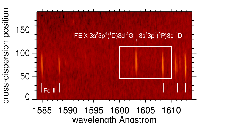
Figure 2.— A close-up of the region containing a record of the Fe X lines of interest. Several lines of Fe II are seen in this figure.

We found just one exposure of sufficient quality to perform the necessary measurement, an exposure from January 9th 1974 beginning at 18:41 UT, catalog number 3B158_007, a 19 minute 59 second exposure. Other promising exposures proved to be have significant chromospheric contamination (3B153_005 for example) or were simply under-exposed (3B160_004).

Figure 2 shows a magnified view of the 1603 Å region, the box shows the same region indicated in Figure 5 (shown at the end of this paper) showing the mid-section of the scanned plate obtained from the NRL data repository. Various spectral lines are shown, including lines used to determine a relative wavelength scale and other prominent and well-known UV lines.

We calibrated the spectrograph’s wavelength scale using lines of Si III (1206.510 Å), C II (1334.535), Si IV (1393.755 and 1402.770), C IV (1548.202, 1550.774), O III (1666.153) Al II (1670.787), with lines of Fe II at 1584.949,1588.286,1608.456,1612.802 Å clustered near 1603 Å. (Wavelengths are from the compilation of Sandlin et al., 1986). We fitted wavelength $\lambda$ to a second order polynomial in position $x$, with the result

$$\lambda=958.95258+ax+bx^{2},$$ (2)

where $a=0.034635388$ and $b=-1.6092831\times 10^{-10}$. with residuals ($\pm 1\sigma$) of 0.02 Å across the entire wavelength range. The residual corresponds to an uncertainty of 0.7 cm^-1 wave-numbers. We assumed that the intensity of the 1603 Fe X blend lies within the linear part of the intensity-density curve, because various lines of Fe II with the same photographic densities appearing to be compatible with optically thin intensities. The intensities were also derived from Fe II line profiles, assumed to be single Gaussians, using photographic density $\rho=\alpha+\beta I+\gamma I^{2}$, and solving for $a,b$ and $c$ from these lines. Then $I$ was solved at neighboring wavelengths for the Fe X transitions. This procedure reduced slightly the lower intensity values at the base of the lines, without changing the results significantly.

We do not know widths of Fe X lines that are unblended, nor do we know the precise wavelength of Fe X lines on the wavelength scale above. Therefore the unresolved FS can only be derived as an upper limit by comparing the observed data with the two lines, estimating for the FS splitting itself (or by a least-squares optimization outlined below). In making these comparisons, we adopted the optically thin ratio of 2.09 for the two lines from CHIANTI (Young et al., 2016). Some typical profiles are illustrated in Figure 3.

Figure 3.— Observed profiles and fits are shown for a specified line width of 0.23 Å, of the 1603.2 Å region of the S082B data obtained above the solar limb. The solid line shows the S082B data, the dotted lines the two components of the Fe X transitions in their optically thin ratio, the dot-dashed lines the total modeled emission for the given FS splitting. The panel labeled “4 cm^-1” shows an acceptable by-eye fit, yielding a FS splitting close to 4 cm^-1. The other panels show the fits, with residuals at least 10 times higher, for splitting values of 1, 7, and 10 cm^-1. For values of FS splitting near and below the line width ($\equiv 8$ cm^-1) there is some redundancy between FS splitting and line width.

The figure shows observed profiles over-plotted with models with a given (1/e) width of 0.23 Å (taken from the optimization calculation below) for four values of the FS splitting. The figure suggests a FS splitting value of $\approx 4$, certainly $\mathrel{\hbox to0.0pt{\lower 3.7pt\hbox{$\sim$} \hss}\raise 1.7pt\hbox{$<$}}7$ cm^-1. The variances, sum of model minus data squared evaluated over the fit to a 1 Å wide band centered at the line, are 2.5, 3 and 9 times the optimal value for 1, 7 and 10 cm^-1 respectively.

Table 1Atomic data for Fe X

Level	Designation	Energy cm-1
0	$3s^{2}3p^{5}{\rm\ {}^{2}P^{o}_{\mathrm{3/2}}}$	0.0
1	$3s^{2}3p^{5}{\rm\ {}^{2}P^{o}_{\mathrm{1/2}}}$	15683.1
2	$3s3p^{6}{\rm\ {}^{2}S_{\mathrm{1/2}}}$	289236
3	$3s^{2}3p^{4}({\rm{}^{3}P})3d{\rm\ {}^{4}D_{\mathrm{7/2}}}$	388710†
4	$3s^{2}3p^{4}({\rm{}^{3}P})3d{\rm\ {}^{4}D_{\mathrm{5/2}}}$	388713.5
5	$3s^{2}3p^{4}({\rm{}^{3}P})3d{\rm\ {}^{4}D_{\mathrm{3/2}}}$	390019
6	$3s^{2}3p^{4}({\rm{}^{3}P})3d{\rm\ {}^{4}D_{\mathrm{1/2}}}$	391554
14	$3s^{2}3p^{4}({\rm{}^{1}D})3d{\rm\ {}^{2}G_{\mathrm{7/2}}}$	451083

Transitions
Type $\lambda$ up lo A gf br Å sec^-1 IC 257.259 4 0 $4.4(6)$ $2.6(-4)$ 1 M2 257.261^† 3 0 47 $3.726(-9)$ 1 MIT 257.261^† 3 0 $3.1(-4){B^{2}}^{\ddagger}$ … 1 IC 256.398 5 0 $7.7(6)$ $3.0(-4)$ 0.98 IC 255.393 6 0 $5.9(6)$ $1.2(-4)$ 0.39 M2 268.075 4 1 $1.0(1)$ $6.7(-10)$ $2.3(-6)$ IC 267.140 5 1 $1.3(5)$ $5.7(-6)$ 0.017 IC 266.049 6 1 $9.4(6)$ $2.0(-4)$ 0.61 M2 1603.348 14 4 9.2 2.8(-8) 0.14 M2 1603.260${\dagger}$ 14 3 19.2 5.9(-8) 0.29

The notation used for the transitions is $X.Y(Z)\equiv X.Y\times 10^{Z}$, the quantity “br” is the radiative branching ratio. Data are from the CHIANTI database (Young et al., 2016), except for the following: ^†Energy level set to 3.5 cm^-1 from the $J=5/2$ level. ^‡Computed by summing all $M$ substates from equation (4) of Li et al. (2015), using a splitting of 3.5 cm^-1, with $B$ measured in G. “IC” is a spin-forbidden intersystem electric dipole transition, “M2” a magnetic dipole transition, “MIT” a magnetically-induced transition.

A trade-off exists between line-width and FS splitting: the larger the width, the lower the splitting needed to fit the same data. Therefore, we can place only an upper limit on the FS splitting from this analysis of $\mathrel{\hbox to0.0pt{\lower 3.7pt\hbox{$\sim$} \hss}\raise 1.7pt\hbox{$<$}}4\pm 3$ cm^-1. But we can go a step further. While the data are photographic and subject to non-linearities in photographic density vs. intensity, we nevertheless performed a formal analysis of variances by fitting the two lines and varying the strong line’s wavelength, line widths and the FS splitting. Both lines were given the same width and the ratio of the intensities was fixed at 2.09. The pikaia genetic algorithm was used (Charbonneau, 1995). Figure 4 shows the $\chi^{2}$ surface as a function of width and FS splitting. We adopted a constant value for the observational error across the line profiles for the $\chi^{2}$ calculation, because the photographic densities lie on top of a large pedestal (equivalent to a dark current). We multiplied the errors by Gaussian functions centered near the obvious blends to either side of the core Fe X emission, to give higher weight to the fits nearer the cores of the Fe X lines of interest. We use the locus of contour level 2 (2$\times$ the minimum $\chi^{2}$) to estimate the error bars in width and FS splitting. We find $8.3\pm 0.6$ and $3.6\pm 1.8$ cm^-1 respectively, using this criterion. These error bars are difficult to justify, they depend on our assumption on the observational errors. We made additional experiments with different observational error weightings. They might reasonably be $1.5\times$ larger, so our final conservative estimates are $8.3\pm 0.9$ and $3.6\pm 2.7$ respectively. Lastly, we found the central wavelength of the stronger transition, on the scale defined using the mix of chromospheric and transition region lines, to be 1603.25 $\pm 0.02$ Å.

Figure 4.— Normalized $\chi^{2}$ values are shown as a function of line width and FS splitting for a model where the two lines have the same line width and an intensity ratio of 2.09:1. The smallest value is set to 1.

The value of $3.6\pm 2.7$ cm^-1 is an independent verification of the small estimate of the splitting $\approx 3.5$ cm^-1 obtained entirely independently by Li et al. (2016) from the Shanghai EBIT device. Our work rejects some of the larger values examined by Li et al. (2015). The small value of the splitting found here also confirms that the line ratios identified by Li et al. (2015) can in principle be used to derive interesting values of the coronal magnetic field strength over active regions.

Finally, we remind the reader that diagnosis of magnetic fields with the MIT technique faces challenges of blended lines and of dependence of line ratios on plasma density (see Figure 6 of Li et al., 2015). Work is in preparation discussing these issues.

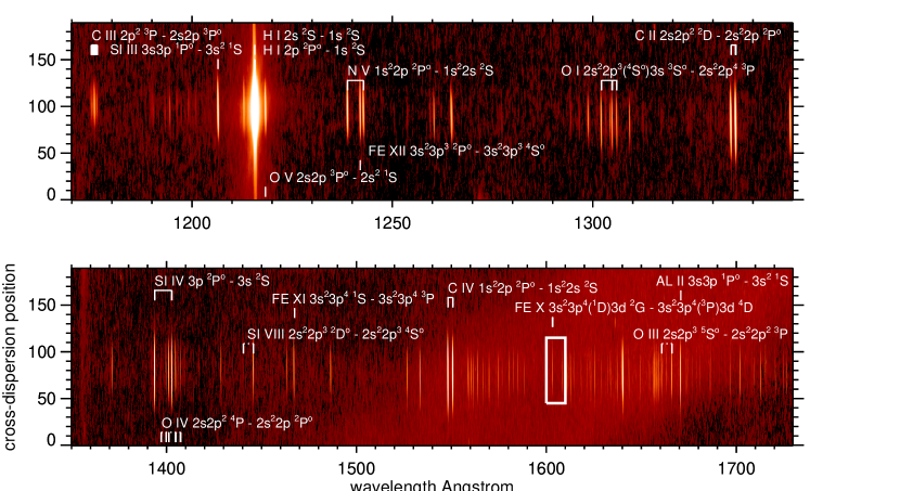
Figure 5.— Raw S082B image with wavelength scale calibrated as described in the text. The image shown is an off-limb exposure, catalog number 3B158_007, a 19 minute 59 second exposure obtained on January 9th 1974 beginning at 18:41 UT. The “intensity” scale shown on the right is photographic density. The images of the spectrograph slit are seen along the abscissa. But because the slit was not in a solar image plane, there is no solar information in the slit direction.

References

- Arnaud and Raymond (1992) Arnaud, M. and Raymond, J.: 1992, Astrophys. J. 398, 394
- Bartoe et al. (1977) Bartoe, J.-D. F., Brueckner, G. E., Purcell, J. D., and Tousey, R.: 1977, Applied Optics 16, 879
- Billings (1966) Billings, D. E.: 1966, A guide to the solar corona, Academic Press, New York
- Burgess and Tully (1992) Burgess, A. and Tully, J. A.: 1992, Astron. Astrophys. 254, 436
- Charbonneau (1995) Charbonneau, P.: 1995, Astrophys. J. Suppl. Ser. 101, 309
- Cheng et al. (1979) Cheng, C.-C., Doschek, G. A., and Feldman, U.: 1979, Astrophys. J. 227, 1037
- Grumer et al. (2014) Grumer, J., Brage, T., Andersson, M., Li, J., Jönsson, P., Li, W., Yang, Y., Hutton, R., and Zou, Y.: 2014, Physica Scripta 89(11), 114002
- Jordan (1969) Jordan, C.: 1969, Mon. Not. R. Astron. Soc. 142, 501
- Kiepenheuer (1953) Kiepenheuer, K. O.: 1953, in G. P. Kuiper (Ed.), The Sun, Chicago University Press, Chicago, p. 322
- Li et al. (2015) Li, W., Grumer, J., Yang, Y., Brage, T., Yao, K., Chen, C., Watanabe, T., Jönsson, P., Lundstedt, H., Hutton, R., and Zou, Y.: 2015, Astrophys. J. 807, 69
- Li et al. (2016) Li, W., Yang, Y., Tu, B., Xiao, J., Grumer, J., Brage, T., Watanabe, T., Hutton, R., and Zou, Y.: 2016, Astrophys. J. 826, 219
- Sandlin et al. (1986) Sandlin, G. D., Bartoe, J.-D. F., Brueckner, G. E., Tousey, R., and VanHoosier, M. E.: 1986, Astrophys. J. Suppl. Ser. 61, 801
- Seaton (1962) Seaton, M. J.: 1962, in D. R. Bates (Ed.), Atomic and Molecular Processes, Academic Press, New York, 11
- Young et al. (2016) Young, P. R., Dere, K. P., Landi, E., Del Zanna, G., and Mason, H. E.: 2016, Journal of Physics B Atomic Molecular Physics 49(7), 074009