^†^†thanks: Earthquake Research Institute, University of Tokyo, Bunkyo, Tokyo 113-0032, Japan

IceCube Collaboration

Measurement of Atmospheric Neutrino Oscillations at 6-56 GeV with IceCube DeepCore

M. G. Aartsen Department of Physics, University of Adelaide, Adelaide, 5005, Australia M. Ackermann DESY, D-15738 Zeuthen, Germany J. Adams Dept. of Physics and Astronomy, University of Canterbury, Private Bag 4800, Christchurch, New Zealand J. A. Aguilar Université Libre de Bruxelles, Science Faculty CP230, B-1050 Brussels, Belgium M. Ahlers Niels Bohr Institute, University of Copenhagen, DK-2100 Copenhagen, Denmark M. Ahrens Oskar Klein Centre and Dept. of Physics, Stockholm University, SE-10691 Stockholm, Sweden I. Al Samarai Département de physique nucléaire et corpusculaire, Université de Genève, CH-1211 Genève, Switzerland D. Altmann Erlangen Centre for Astroparticle Physics, Friedrich-Alexander-Universität Erlangen-Nürnberg, D-91058 Erlangen, Germany K. Andeen Department of Physics, Marquette University, Milwaukee, WI, 53201, USA T. Anderson Dept. of Physics, Pennsylvania State University, University Park, PA 16802, USA I. Ansseau Université Libre de Bruxelles, Science Faculty CP230, B-1050 Brussels, Belgium G. Anton Erlangen Centre for Astroparticle Physics, Friedrich-Alexander-Universität Erlangen-Nürnberg, D-91058 Erlangen, Germany C. Argüelles Dept. of Physics, Massachusetts Institute of Technology, Cambridge, MA 02139, USA J. Auffenberg III. Physikalisches Institut, RWTH Aachen University, D-52056 Aachen, Germany S. Axani Dept. of Physics, Massachusetts Institute of Technology, Cambridge, MA 02139, USA H. Bagherpour Dept. of Physics and Astronomy, University of Canterbury, Private Bag 4800, Christchurch, New Zealand X. Bai Physics Department, South Dakota School of Mines and Technology, Rapid City, SD 57701, USA J. P. Barron Dept. of Physics, University of Alberta, Edmonton, Alberta, Canada T6G 2E1 S. W. Barwick Dept. of Physics and Astronomy, University of California, Irvine, CA 92697, USA V. Baum Institute of Physics, University of Mainz, Staudinger Weg 7, D-55099 Mainz, Germany R. Bay Dept. of Physics, University of California, Berkeley, CA 94720, USA J. J. Beatty Dept. of Physics and Center for Cosmology and Astro-Particle Physics, Ohio State University, Columbus, OH 43210, USA Dept. of Astronomy, Ohio State University, Columbus, OH 43210, USA J. Becker Tjus Fakultät für Physik & Astronomie, Ruhr-Universität Bochum, D-44780 Bochum, Germany K.-H. Becker Dept. of Physics, University of Wuppertal, D-42119 Wuppertal, Germany S. BenZvi Dept. of Physics and Astronomy, University of Rochester, Rochester, NY 14627, USA D. Berley Dept. of Physics, University of Maryland, College Park, MD 20742, USA E. Bernardini DESY, D-15738 Zeuthen, Germany D. Z. Besson Dept. of Physics and Astronomy, University of Kansas, Lawrence, KS 66045, USA G. Binder Lawrence Berkeley National Laboratory, Berkeley, CA 94720, USA Dept. of Physics, University of California, Berkeley, CA 94720, USA D. Bindig Dept. of Physics, University of Wuppertal, D-42119 Wuppertal, Germany E. Blaufuss Dept. of Physics, University of Maryland, College Park, MD 20742, USA S. Blot DESY, D-15738 Zeuthen, Germany C. Bohm Oskar Klein Centre and Dept. of Physics, Stockholm University, SE-10691 Stockholm, Sweden M. Börner Dept. of Physics, TU Dortmund University, D-44221 Dortmund, Germany F. Bos Fakultät für Physik & Astronomie, Ruhr-Universität Bochum, D-44780 Bochum, Germany D. Bose Dept. of Physics, Sungkyunkwan University, Suwon 440-746, Korea S. Böser Institute of Physics, University of Mainz, Staudinger Weg 7, D-55099 Mainz, Germany O. Botner Dept. of Physics and Astronomy, Uppsala University, Box 516, S-75120 Uppsala, Sweden J. Bourbeau Dept. of Physics and Wisconsin IceCube Particle Astrophysics Center, University of Wisconsin, Madison, WI 53706, USA F. Bradascio DESY, D-15738 Zeuthen, Germany J. Braun Dept. of Physics and Wisconsin IceCube Particle Astrophysics Center, University of Wisconsin, Madison, WI 53706, USA L. Brayeur Vrije Universiteit Brussel (VUB), Dienst ELEM, B-1050 Brussels, Belgium M. Brenzke III. Physikalisches Institut, RWTH Aachen University, D-52056 Aachen, Germany H.-P. Bretz DESY, D-15738 Zeuthen, Germany S. Bron Département de physique nucléaire et corpusculaire, Université de Genève, CH-1211 Genève, Switzerland J. Brostean-Kaiser DESY, D-15738 Zeuthen, Germany A. Burgman Dept. of Physics and Astronomy, Uppsala University, Box 516, S-75120 Uppsala, Sweden T. Carver Département de physique nucléaire et corpusculaire, Université de Genève, CH-1211 Genève, Switzerland J. Casey Dept. of Physics and Wisconsin IceCube Particle Astrophysics Center, University of Wisconsin, Madison, WI 53706, USA M. Casier Vrije Universiteit Brussel (VUB), Dienst ELEM, B-1050 Brussels, Belgium E. Cheung Dept. of Physics, University of Maryland, College Park, MD 20742, USA D. Chirkin Dept. of Physics and Wisconsin IceCube Particle Astrophysics Center, University of Wisconsin, Madison, WI 53706, USA A. Christov Département de physique nucléaire et corpusculaire, Université de Genève, CH-1211 Genève, Switzerland K. Clark SNOLAB, 1039 Regional Road 24, Creighton Mine 9, Lively, ON, Canada P3Y 1N2 L. Classen Institut für Kernphysik, Westfälische Wilhelms-Universität Münster, D-48149 Münster, Germany S. Coenders Physik-department, Technische Universität München, D-85748 Garching, Germany G. H. Collin Dept. of Physics, Massachusetts Institute of Technology, Cambridge, MA 02139, USA J. M. Conrad Dept. of Physics, Massachusetts Institute of Technology, Cambridge, MA 02139, USA D. F. Cowen Dept. of Physics, Pennsylvania State University, University Park, PA 16802, USA Dept. of Astronomy and Astrophysics, Pennsylvania State University, University Park, PA 16802, USA R. Cross Dept. of Physics and Astronomy, University of Rochester, Rochester, NY 14627, USA M. Day Dept. of Physics and Wisconsin IceCube Particle Astrophysics Center, University of Wisconsin, Madison, WI 53706, USA J. P. A. M. de André Dept. of Physics and Astronomy, Michigan State University, East Lansing, MI 48824, USA C. De Clercq Vrije Universiteit Brussel (VUB), Dienst ELEM, B-1050 Brussels, Belgium J. J. DeLaunay Dept. of Physics, Pennsylvania State University, University Park, PA 16802, USA H. Dembinski Bartol Research Institute and Dept. of Physics and Astronomy, University of Delaware, Newark, DE 19716, USA S. De Ridder Dept. of Physics and Astronomy, University of Gent, B-9000 Gent, Belgium P. Desiati Dept. of Physics and Wisconsin IceCube Particle Astrophysics Center, University of Wisconsin, Madison, WI 53706, USA K. D. de Vries Vrije Universiteit Brussel (VUB), Dienst ELEM, B-1050 Brussels, Belgium G. de Wasseige Vrije Universiteit Brussel (VUB), Dienst ELEM, B-1050 Brussels, Belgium M. de With Institut für Physik, Humboldt-Universität zu Berlin, D-12489 Berlin, Germany T. DeYoung Dept. of Physics and Astronomy, Michigan State University, East Lansing, MI 48824, USA J. C. Díaz-Vélez Dept. of Physics and Wisconsin IceCube Particle Astrophysics Center, University of Wisconsin, Madison, WI 53706, USA V. di Lorenzo Institute of Physics, University of Mainz, Staudinger Weg 7, D-55099 Mainz, Germany H. Dujmovic Dept. of Physics, Sungkyunkwan University, Suwon 440-746, Korea J. P. Dumm Oskar Klein Centre and Dept. of Physics, Stockholm University, SE-10691 Stockholm, Sweden M. Dunkman Dept. of Physics, Pennsylvania State University, University Park, PA 16802, USA B. Eberhardt Institute of Physics, University of Mainz, Staudinger Weg 7, D-55099 Mainz, Germany T. Ehrhardt Institute of Physics, University of Mainz, Staudinger Weg 7, D-55099 Mainz, Germany B. Eichmann Fakultät für Physik & Astronomie, Ruhr-Universität Bochum, D-44780 Bochum, Germany P. Eller Dept. of Physics, Pennsylvania State University, University Park, PA 16802, USA P. A. Evenson Bartol Research Institute and Dept. of Physics and Astronomy, University of Delaware, Newark, DE 19716, USA S. Fahey Dept. of Physics and Wisconsin IceCube Particle Astrophysics Center, University of Wisconsin, Madison, WI 53706, USA A. R. Fazely Dept. of Physics, Southern University, Baton Rouge, LA 70813, USA J. Felde Dept. of Physics, University of Maryland, College Park, MD 20742, USA K. Filimonov Dept. of Physics, University of California, Berkeley, CA 94720, USA C. Finley Oskar Klein Centre and Dept. of Physics, Stockholm University, SE-10691 Stockholm, Sweden S. Flis Oskar Klein Centre and Dept. of Physics, Stockholm University, SE-10691 Stockholm, Sweden A. Franckowiak DESY, D-15738 Zeuthen, Germany E. Friedman Dept. of Physics, University of Maryland, College Park, MD 20742, USA T. Fuchs Dept. of Physics, TU Dortmund University, D-44221 Dortmund, Germany T. K. Gaisser Bartol Research Institute and Dept. of Physics and Astronomy, University of Delaware, Newark, DE 19716, USA J. Gallagher Dept. of Astronomy, University of Wisconsin, Madison, WI 53706, USA L. Gerhardt Lawrence Berkeley National Laboratory, Berkeley, CA 94720, USA K. Ghorbani Dept. of Physics and Wisconsin IceCube Particle Astrophysics Center, University of Wisconsin, Madison, WI 53706, USA W. Giang Dept. of Physics, University of Alberta, Edmonton, Alberta, Canada T6G 2E1 T. Glauch III. Physikalisches Institut, RWTH Aachen University, D-52056 Aachen, Germany T. Glüsenkamp Erlangen Centre for Astroparticle Physics, Friedrich-Alexander-Universität Erlangen-Nürnberg, D-91058 Erlangen, Germany A. Goldschmidt Lawrence Berkeley National Laboratory, Berkeley, CA 94720, USA J. G. Gonzalez Bartol Research Institute and Dept. of Physics and Astronomy, University of Delaware, Newark, DE 19716, USA D. Grant Dept. of Physics, University of Alberta, Edmonton, Alberta, Canada T6G 2E1 Z. Griffith Dept. of Physics and Wisconsin IceCube Particle Astrophysics Center, University of Wisconsin, Madison, WI 53706, USA C. Haack III. Physikalisches Institut, RWTH Aachen University, D-52056 Aachen, Germany A. Hallgren Dept. of Physics and Astronomy, Uppsala University, Box 516, S-75120 Uppsala, Sweden F. Halzen Dept. of Physics and Wisconsin IceCube Particle Astrophysics Center, University of Wisconsin, Madison, WI 53706, USA K. Hanson Dept. of Physics and Wisconsin IceCube Particle Astrophysics Center, University of Wisconsin, Madison, WI 53706, USA D. Hebecker Institut für Physik, Humboldt-Universität zu Berlin, D-12489 Berlin, Germany D. Heereman Université Libre de Bruxelles, Science Faculty CP230, B-1050 Brussels, Belgium K. Helbing Dept. of Physics, University of Wuppertal, D-42119 Wuppertal, Germany R. Hellauer Dept. of Physics, University of Maryland, College Park, MD 20742, USA S. Hickford Dept. of Physics, University of Wuppertal, D-42119 Wuppertal, Germany J. Hignight Dept. of Physics and Astronomy, Michigan State University, East Lansing, MI 48824, USA G. C. Hill Department of Physics, University of Adelaide, Adelaide, 5005, Australia K. D. Hoffman Dept. of Physics, University of Maryland, College Park, MD 20742, USA R. Hoffmann Dept. of Physics, University of Wuppertal, D-42119 Wuppertal, Germany B. Hokanson-Fasig Dept. of Physics and Wisconsin IceCube Particle Astrophysics Center, University of Wisconsin, Madison, WI 53706, USA K. Hoshina Dept. of Physics and Wisconsin IceCube Particle Astrophysics Center, University of Wisconsin, Madison, WI 53706, USA F. Huang Dept. of Physics, Pennsylvania State University, University Park, PA 16802, USA M. Huber Physik-department, Technische Universität München, D-85748 Garching, Germany K. Hultqvist Oskar Klein Centre and Dept. of Physics, Stockholm University, SE-10691 Stockholm, Sweden M. Hünnefeld Dept. of Physics, TU Dortmund University, D-44221 Dortmund, Germany S. In Dept. of Physics, Sungkyunkwan University, Suwon 440-746, Korea A. Ishihara Dept. of Physics and Institute for Global Prominent Research, Chiba University, Chiba 263-8522, Japan E. Jacobi DESY, D-15738 Zeuthen, Germany G. S. Japaridze CTSPS, Clark-Atlanta University, Atlanta, GA 30314, USA M. Jeong Dept. of Physics, Sungkyunkwan University, Suwon 440-746, Korea K. Jero Dept. of Physics and Wisconsin IceCube Particle Astrophysics Center, University of Wisconsin, Madison, WI 53706, USA B. J. P. Jones Dept. of Physics, University of Texas at Arlington, 502 Yates St., Science Hall Rm 108, Box 19059, Arlington, TX 76019, USA P. Kalaczynski III. Physikalisches Institut, RWTH Aachen University, D-52056 Aachen, Germany W. Kang Dept. of Physics, Sungkyunkwan University, Suwon 440-746, Korea A. Kappes Institut für Kernphysik, Westfälische Wilhelms-Universität Münster, D-48149 Münster, Germany T. Karg DESY, D-15738 Zeuthen, Germany A. Karle Dept. of Physics and Wisconsin IceCube Particle Astrophysics Center, University of Wisconsin, Madison, WI 53706, USA U. Katz Erlangen Centre for Astroparticle Physics, Friedrich-Alexander-Universität Erlangen-Nürnberg, D-91058 Erlangen, Germany M. Kauer Dept. of Physics and Wisconsin IceCube Particle Astrophysics Center, University of Wisconsin, Madison, WI 53706, USA A. Keivani Dept. of Physics, Pennsylvania State University, University Park, PA 16802, USA J. L. Kelley Dept. of Physics and Wisconsin IceCube Particle Astrophysics Center, University of Wisconsin, Madison, WI 53706, USA A. Kheirandish Dept. of Physics and Wisconsin IceCube Particle Astrophysics Center, University of Wisconsin, Madison, WI 53706, USA J. Kim Dept. of Physics, Sungkyunkwan University, Suwon 440-746, Korea M. Kim Dept. of Physics and Institute for Global Prominent Research, Chiba University, Chiba 263-8522, Japan T. Kintscher DESY, D-15738 Zeuthen, Germany J. Kiryluk Dept. of Physics and Astronomy, Stony Brook University, Stony Brook, NY 11794-3800, USA T. Kittler Erlangen Centre for Astroparticle Physics, Friedrich-Alexander-Universität Erlangen-Nürnberg, D-91058 Erlangen, Germany S. R. Klein Lawrence Berkeley National Laboratory, Berkeley, CA 94720, USA Dept. of Physics, University of California, Berkeley, CA 94720, USA G. Kohnen Université de Mons, 7000 Mons, Belgium R. Koirala Bartol Research Institute and Dept. of Physics and Astronomy, University of Delaware, Newark, DE 19716, USA H. Kolanoski Institut für Physik, Humboldt-Universität zu Berlin, D-12489 Berlin, Germany L. Köpke Institute of Physics, University of Mainz, Staudinger Weg 7, D-55099 Mainz, Germany C. Kopper Dept. of Physics, University of Alberta, Edmonton, Alberta, Canada T6G 2E1 S. Kopper Dept. of Physics and Astronomy, University of Alabama, Tuscaloosa, AL 35487, USA J. P. Koschinsky III. Physikalisches Institut, RWTH Aachen University, D-52056 Aachen, Germany D. J. Koskinen Niels Bohr Institute, University of Copenhagen, DK-2100 Copenhagen, Denmark M. Kowalski Institut für Physik, Humboldt-Universität zu Berlin, D-12489 Berlin, Germany DESY, D-15738 Zeuthen, Germany K. Krings Physik-department, Technische Universität München, D-85748 Garching, Germany M. Kroll Fakultät für Physik & Astronomie, Ruhr-Universität Bochum, D-44780 Bochum, Germany G. Krückl Institute of Physics, University of Mainz, Staudinger Weg 7, D-55099 Mainz, Germany J. Kunnen Vrije Universiteit Brussel (VUB), Dienst ELEM, B-1050 Brussels, Belgium S. Kunwar DESY, D-15738 Zeuthen, Germany N. Kurahashi Dept. of Physics, Drexel University, 3141 Chestnut Street, Philadelphia, PA 19104, USA T. Kuwabara Dept. of Physics and Institute for Global Prominent Research, Chiba University, Chiba 263-8522, Japan A. Kyriacou Department of Physics, University of Adelaide, Adelaide, 5005, Australia M. Labare Dept. of Physics and Astronomy, University of Gent, B-9000 Gent, Belgium J. L. Lanfranchi Dept. of Physics, Pennsylvania State University, University Park, PA 16802, USA M. J. Larson Niels Bohr Institute, University of Copenhagen, DK-2100 Copenhagen, Denmark F. Lauber Dept. of Physics, University of Wuppertal, D-42119 Wuppertal, Germany D. Lennarz Dept. of Physics and Astronomy, Michigan State University, East Lansing, MI 48824, USA M. Lesiak-Bzdak Dept. of Physics and Astronomy, Stony Brook University, Stony Brook, NY 11794-3800, USA M. Leuermann III. Physikalisches Institut, RWTH Aachen University, D-52056 Aachen, Germany Q. R. Liu Dept. of Physics and Wisconsin IceCube Particle Astrophysics Center, University of Wisconsin, Madison, WI 53706, USA L. Lu Dept. of Physics and Institute for Global Prominent Research, Chiba University, Chiba 263-8522, Japan J. Lünemann Vrije Universiteit Brussel (VUB), Dienst ELEM, B-1050 Brussels, Belgium W. Luszczak Dept. of Physics and Wisconsin IceCube Particle Astrophysics Center, University of Wisconsin, Madison, WI 53706, USA J. Madsen Dept. of Physics, University of Wisconsin, River Falls, WI 54022, USA G. Maggi Vrije Universiteit Brussel (VUB), Dienst ELEM, B-1050 Brussels, Belgium K. B. M. Mahn Dept. of Physics and Astronomy, Michigan State University, East Lansing, MI 48824, USA S. Mancina Dept. of Physics and Wisconsin IceCube Particle Astrophysics Center, University of Wisconsin, Madison, WI 53706, USA R. Maruyama Dept. of Physics, Yale University, New Haven, CT 06520, USA K. Mase Dept. of Physics and Institute for Global Prominent Research, Chiba University, Chiba 263-8522, Japan R. Maunu Dept. of Physics, University of Maryland, College Park, MD 20742, USA F. McNally Dept. of Physics and Wisconsin IceCube Particle Astrophysics Center, University of Wisconsin, Madison, WI 53706, USA K. Meagher Université Libre de Bruxelles, Science Faculty CP230, B-1050 Brussels, Belgium M. Medici Niels Bohr Institute, University of Copenhagen, DK-2100 Copenhagen, Denmark M. Meier Dept. of Physics, TU Dortmund University, D-44221 Dortmund, Germany T. Menne Dept. of Physics, TU Dortmund University, D-44221 Dortmund, Germany G. Merino Dept. of Physics and Wisconsin IceCube Particle Astrophysics Center, University of Wisconsin, Madison, WI 53706, USA T. Meures Université Libre de Bruxelles, Science Faculty CP230, B-1050 Brussels, Belgium S. Miarecki Lawrence Berkeley National Laboratory, Berkeley, CA 94720, USA Dept. of Physics, University of California, Berkeley, CA 94720, USA J. Micallef Dept. of Physics and Astronomy, Michigan State University, East Lansing, MI 48824, USA G. Momenté Institute of Physics, University of Mainz, Staudinger Weg 7, D-55099 Mainz, Germany T. Montaruli Département de physique nucléaire et corpusculaire, Université de Genève, CH-1211 Genève, Switzerland R. W. Moore Dept. of Physics, University of Alberta, Edmonton, Alberta, Canada T6G 2E1 M. Moulai Dept. of Physics, Massachusetts Institute of Technology, Cambridge, MA 02139, USA R. Nahnhauer DESY, D-15738 Zeuthen, Germany P. Nakarmi Dept. of Physics and Astronomy, University of Alabama, Tuscaloosa, AL 35487, USA U. Naumann Dept. of Physics, University of Wuppertal, D-42119 Wuppertal, Germany G. Neer Dept. of Physics and Astronomy, Michigan State University, East Lansing, MI 48824, USA H. Niederhausen Dept. of Physics and Astronomy, Stony Brook University, Stony Brook, NY 11794-3800, USA S. C. Nowicki Dept. of Physics, University of Alberta, Edmonton, Alberta, Canada T6G 2E1 D. R. Nygren Lawrence Berkeley National Laboratory, Berkeley, CA 94720, USA A. Obertacke Pollmann Dept. of Physics, University of Wuppertal, D-42119 Wuppertal, Germany A. Olivas Dept. of Physics, University of Maryland, College Park, MD 20742, USA A. O’Murchadha Université Libre de Bruxelles, Science Faculty CP230, B-1050 Brussels, Belgium T. Palczewski Lawrence Berkeley National Laboratory, Berkeley, CA 94720, USA Dept. of Physics, University of California, Berkeley, CA 94720, USA H. Pandya Bartol Research Institute and Dept. of Physics and Astronomy, University of Delaware, Newark, DE 19716, USA D. V. Pankova Dept. of Physics, Pennsylvania State University, University Park, PA 16802, USA P. Peiffer Institute of Physics, University of Mainz, Staudinger Weg 7, D-55099 Mainz, Germany J. A. Pepper Dept. of Physics and Astronomy, University of Alabama, Tuscaloosa, AL 35487, USA C. Pérez de los Heros Dept. of Physics and Astronomy, Uppsala University, Box 516, S-75120 Uppsala, Sweden D. Pieloth Dept. of Physics, TU Dortmund University, D-44221 Dortmund, Germany E. Pinat Université Libre de Bruxelles, Science Faculty CP230, B-1050 Brussels, Belgium M. Plum Department of Physics, Marquette University, Milwaukee, WI, 53201, USA P. B. Price Dept. of Physics, University of California, Berkeley, CA 94720, USA G. T. Przybylski Lawrence Berkeley National Laboratory, Berkeley, CA 94720, USA C. Raab Université Libre de Bruxelles, Science Faculty CP230, B-1050 Brussels, Belgium L. Rädel III. Physikalisches Institut, RWTH Aachen University, D-52056 Aachen, Germany M. Rameez Niels Bohr Institute, University of Copenhagen, DK-2100 Copenhagen, Denmark K. Rawlins Dept. of Physics and Astronomy, University of Alaska Anchorage, 3211 Providence Dr., Anchorage, AK 99508, USA I. C. Rea Physik-department, Technische Universität München, D-85748 Garching, Germany R. Reimann III. Physikalisches Institut, RWTH Aachen University, D-52056 Aachen, Germany B. Relethford Dept. of Physics, Drexel University, 3141 Chestnut Street, Philadelphia, PA 19104, USA M. Relich Dept. of Physics and Institute for Global Prominent Research, Chiba University, Chiba 263-8522, Japan E. Resconi Physik-department, Technische Universität München, D-85748 Garching, Germany W. Rhode Dept. of Physics, TU Dortmund University, D-44221 Dortmund, Germany M. Richman Dept. of Physics, Drexel University, 3141 Chestnut Street, Philadelphia, PA 19104, USA S. Robertson Department of Physics, University of Adelaide, Adelaide, 5005, Australia M. Rongen III. Physikalisches Institut, RWTH Aachen University, D-52056 Aachen, Germany C. Rott Dept. of Physics, Sungkyunkwan University, Suwon 440-746, Korea T. Ruhe Dept. of Physics, TU Dortmund University, D-44221 Dortmund, Germany D. Ryckbosch Dept. of Physics and Astronomy, University of Gent, B-9000 Gent, Belgium D. Rysewyk Dept. of Physics and Astronomy, Michigan State University, East Lansing, MI 48824, USA T. Sälzer III. Physikalisches Institut, RWTH Aachen University, D-52056 Aachen, Germany S. E. Sanchez Herrera Dept. of Physics, University of Alberta, Edmonton, Alberta, Canada T6G 2E1 A. Sandrock Dept. of Physics, TU Dortmund University, D-44221 Dortmund, Germany J. Sandroos Institute of Physics, University of Mainz, Staudinger Weg 7, D-55099 Mainz, Germany S. Sarkar Niels Bohr Institute, University of Copenhagen, DK-2100 Copenhagen, Denmark Dept. of Physics, University of Oxford, 1 Keble Road, Oxford OX1 3NP, UK S. Sarkar Dept. of Physics, University of Alberta, Edmonton, Alberta, Canada T6G 2E1 K. Satalecka DESY, D-15738 Zeuthen, Germany P. Schlunder Dept. of Physics, TU Dortmund University, D-44221 Dortmund, Germany T. Schmidt Dept. of Physics, University of Maryland, College Park, MD 20742, USA A. Schneider Dept. of Physics and Wisconsin IceCube Particle Astrophysics Center, University of Wisconsin, Madison, WI 53706, USA S. Schoenen III. Physikalisches Institut, RWTH Aachen University, D-52056 Aachen, Germany S. Schöneberg Fakultät für Physik & Astronomie, Ruhr-Universität Bochum, D-44780 Bochum, Germany L. Schumacher III. Physikalisches Institut, RWTH Aachen University, D-52056 Aachen, Germany D. Seckel Bartol Research Institute and Dept. of Physics and Astronomy, University of Delaware, Newark, DE 19716, USA S. Seunarine Dept. of Physics, University of Wisconsin, River Falls, WI 54022, USA J. Soedingrekso Dept. of Physics, TU Dortmund University, D-44221 Dortmund, Germany D. Soldin Dept. of Physics, University of Wuppertal, D-42119 Wuppertal, Germany M. Song Dept. of Physics, University of Maryland, College Park, MD 20742, USA G. M. Spiczak Dept. of Physics, University of Wisconsin, River Falls, WI 54022, USA C. Spiering DESY, D-15738 Zeuthen, Germany J. Stachurska DESY, D-15738 Zeuthen, Germany M. Stamatikos Dept. of Physics and Center for Cosmology and Astro-Particle Physics, Ohio State University, Columbus, OH 43210, USA T. Stanev Bartol Research Institute and Dept. of Physics and Astronomy, University of Delaware, Newark, DE 19716, USA A. Stasik DESY, D-15738 Zeuthen, Germany J. Stettner III. Physikalisches Institut, RWTH Aachen University, D-52056 Aachen, Germany A. Steuer Institute of Physics, University of Mainz, Staudinger Weg 7, D-55099 Mainz, Germany T. Stezelberger Lawrence Berkeley National Laboratory, Berkeley, CA 94720, USA R. G. Stokstad Lawrence Berkeley National Laboratory, Berkeley, CA 94720, USA A. Stößl Dept. of Physics and Institute for Global Prominent Research, Chiba University, Chiba 263-8522, Japan N. L. Strotjohann DESY, D-15738 Zeuthen, Germany G. W. Sullivan Dept. of Physics, University of Maryland, College Park, MD 20742, USA M. Sutherland Dept. of Physics and Center for Cosmology and Astro-Particle Physics, Ohio State University, Columbus, OH 43210, USA I. Taboada School of Physics and Center for Relativistic Astrophysics, Georgia Institute of Technology, Atlanta, GA 30332, USA J. Tatar Lawrence Berkeley National Laboratory, Berkeley, CA 94720, USA Dept. of Physics, University of California, Berkeley, CA 94720, USA F. Tenholt Fakultät für Physik & Astronomie, Ruhr-Universität Bochum, D-44780 Bochum, Germany S. Ter-Antonyan Dept. of Physics, Southern University, Baton Rouge, LA 70813, USA A. Terliuk DESY, D-15738 Zeuthen, Germany G. Tešić Dept. of Physics, Pennsylvania State University, University Park, PA 16802, USA S. Tilav Bartol Research Institute and Dept. of Physics and Astronomy, University of Delaware, Newark, DE 19716, USA P. A. Toale Dept. of Physics and Astronomy, University of Alabama, Tuscaloosa, AL 35487, USA M. N. Tobin Dept. of Physics and Wisconsin IceCube Particle Astrophysics Center, University of Wisconsin, Madison, WI 53706, USA S. Toscano Vrije Universiteit Brussel (VUB), Dienst ELEM, B-1050 Brussels, Belgium D. Tosi Dept. of Physics and Wisconsin IceCube Particle Astrophysics Center, University of Wisconsin, Madison, WI 53706, USA M. Tselengidou Erlangen Centre for Astroparticle Physics, Friedrich-Alexander-Universität Erlangen-Nürnberg, D-91058 Erlangen, Germany C. F. Tung School of Physics and Center for Relativistic Astrophysics, Georgia Institute of Technology, Atlanta, GA 30332, USA A. Turcati Physik-department, Technische Universität München, D-85748 Garching, Germany C. F. Turley Dept. of Physics, Pennsylvania State University, University Park, PA 16802, USA B. Ty Dept. of Physics and Wisconsin IceCube Particle Astrophysics Center, University of Wisconsin, Madison, WI 53706, USA E. Unger Dept. of Physics and Astronomy, Uppsala University, Box 516, S-75120 Uppsala, Sweden M. Usner DESY, D-15738 Zeuthen, Germany J. Vandenbroucke Dept. of Physics and Wisconsin IceCube Particle Astrophysics Center, University of Wisconsin, Madison, WI 53706, USA W. Van Driessche Dept. of Physics and Astronomy, University of Gent, B-9000 Gent, Belgium N. van Eijndhoven Vrije Universiteit Brussel (VUB), Dienst ELEM, B-1050 Brussels, Belgium S. Vanheule Dept. of Physics and Astronomy, University of Gent, B-9000 Gent, Belgium J. van Santen DESY, D-15738 Zeuthen, Germany M. Vehring III. Physikalisches Institut, RWTH Aachen University, D-52056 Aachen, Germany E. Vogel III. Physikalisches Institut, RWTH Aachen University, D-52056 Aachen, Germany M. Vraeghe Dept. of Physics and Astronomy, University of Gent, B-9000 Gent, Belgium C. Walck Oskar Klein Centre and Dept. of Physics, Stockholm University, SE-10691 Stockholm, Sweden A. Wallace Department of Physics, University of Adelaide, Adelaide, 5005, Australia M. Wallraff III. Physikalisches Institut, RWTH Aachen University, D-52056 Aachen, Germany F. D. Wandler Dept. of Physics, University of Alberta, Edmonton, Alberta, Canada T6G 2E1 N. Wandkowsky Dept. of Physics and Wisconsin IceCube Particle Astrophysics Center, University of Wisconsin, Madison, WI 53706, USA A. Waza III. Physikalisches Institut, RWTH Aachen University, D-52056 Aachen, Germany C. Weaver Dept. of Physics, University of Alberta, Edmonton, Alberta, Canada T6G 2E1 M. J. Weiss Dept. of Physics, Pennsylvania State University, University Park, PA 16802, USA C. Wendt Dept. of Physics and Wisconsin IceCube Particle Astrophysics Center, University of Wisconsin, Madison, WI 53706, USA J. Werthebach Dept. of Physics, TU Dortmund University, D-44221 Dortmund, Germany S. Westerhoff Dept. of Physics and Wisconsin IceCube Particle Astrophysics Center, University of Wisconsin, Madison, WI 53706, USA B. J. Whelan Department of Physics, University of Adelaide, Adelaide, 5005, Australia K. Wiebe Institute of Physics, University of Mainz, Staudinger Weg 7, D-55099 Mainz, Germany C. H. Wiebusch III. Physikalisches Institut, RWTH Aachen University, D-52056 Aachen, Germany L. Wille Dept. of Physics and Wisconsin IceCube Particle Astrophysics Center, University of Wisconsin, Madison, WI 53706, USA D. R. Williams Dept. of Physics and Astronomy, University of Alabama, Tuscaloosa, AL 35487, USA L. Wills Dept. of Physics, Drexel University, 3141 Chestnut Street, Philadelphia, PA 19104, USA M. Wolf Dept. of Physics and Wisconsin IceCube Particle Astrophysics Center, University of Wisconsin, Madison, WI 53706, USA J. Wood Dept. of Physics and Wisconsin IceCube Particle Astrophysics Center, University of Wisconsin, Madison, WI 53706, USA T. R. Wood Dept. of Physics, University of Alberta, Edmonton, Alberta, Canada T6G 2E1 E. Woolsey Dept. of Physics, University of Alberta, Edmonton, Alberta, Canada T6G 2E1 K. Woschnagg Dept. of Physics, University of California, Berkeley, CA 94720, USA D. L. Xu Dept. of Physics and Wisconsin IceCube Particle Astrophysics Center, University of Wisconsin, Madison, WI 53706, USA X. W. Xu Dept. of Physics, Southern University, Baton Rouge, LA 70813, USA Y. Xu Dept. of Physics and Astronomy, Stony Brook University, Stony Brook, NY 11794-3800, USA J. P. Yanez Dept. of Physics, University of Alberta, Edmonton, Alberta, Canada T6G 2E1 G. Yodh Dept. of Physics and Astronomy, University of California, Irvine, CA 92697, USA S. Yoshida Dept. of Physics and Institute for Global Prominent Research, Chiba University, Chiba 263-8522, Japan T. Yuan Dept. of Physics and Wisconsin IceCube Particle Astrophysics Center, University of Wisconsin, Madison, WI 53706, USA M. Zoll Oskar Klein Centre and Dept. of Physics, Stockholm University, SE-10691 Stockholm, Sweden analysis@icecube.wisc.edu

Abstract

We present a measurement of the atmospheric neutrino oscillation parameters using three years of data from the IceCube Neutrino Observatory. The DeepCore infill array in the center of IceCube enables detection and reconstruction of neutrinos produced by the interaction of cosmic rays in the Earth’s atmosphere at energies as low as $\sim 5$ GeV. That energy threshold permits measurements of muon neutrino disappearance, over a range of baselines up to the diameter of the Earth, probing the same range of $L/E_{\nu}$ as long-baseline experiments but with substantially higher energy neutrinos. This analysis uses neutrinos from the full sky with reconstructed energies from $5.6$ – $56$ GeV. We measure $\Delta m^{2}_{32}=2.31^{+0.11}_{-0.13}\times 10^{-3}$ eV² and $\sin^{2}\theta_{23}=0.51^{+0.07}_{-0.09}$ , assuming normal neutrino mass ordering. These results are consistent with, and of similar precision to, those from accelerator and reactor-based experiments.

pacs:

Valid PACS appear here

I Introduction

It is well established that the neutrino mass eigenstates do not correspond to the neutrino flavor eigenstates, leading to flavor oscillations as neutrinos propagate through space Fukuda et al. (1998); Ahmad et al. (2001). After traveling a distance $L$ a neutrino of energy $E$ may be detected with a different flavor than it was produced with. In particular, the muon neutrino survival probability is described approximately by

P(\nu_{\mu}\rightarrow\nu_{\mu})\approx 1-4|U_{\mu 3}|^{2}\left(1-|U_{\mu 3}|^{2}\right)\sin^{2}\left(\frac{\Delta m_{32}^{2}L}{4E}\right),

(1)

where $U_{\mu 3}=\sin\theta_{23}\cos\theta_{13}$ is one element of the PMNS Pontecorvo (1957); Maki et al. (1962) matrix $U$ expressed in terms of the mixing angles $\theta_{23}$ and $\theta_{13}$ , $\Delta m^{2}_{32}=m^{2}_{3}-m^{2}_{2}$ is the splitting of the second and third neutrino mass states that drives oscillation on the length and energy scales relevant to this analysis. In addition to the parameters shown in Eq. (1), neutrino oscillations also depend on the parameters $\theta_{12}$ , $\Delta m^{2}_{21}$ and $\delta_{CP}$ , but these have a negligible effect on the data presented in this paper.

Interactions of cosmic rays in the atmosphere Volkova (1980); Barr et al. (2004); Honda et al. (2015) provide a large flux of neutrinos traveling distances ranging from $L\sim 20$ km (vertically down-going) to $L\sim 1.3\times 10^{4}$ km (vertically up-going) to a detector near the Earth’s surface. For up-going neutrinos, there is complete muon neutrino disappearance at energies as high as $\sim 25$ GeV. Given the density of material traversed by these neutrinos, matter effects alter Eq. (1) slightly and must be taken into account Wolfenstein (1978); Petcov (1998); Akhmedov et al. (2007, 2008).

In this letter, we report our measurement of $\theta_{23}$ and $\Delta m_{32}^{2}$ , using the IceCube Observatory to observe oscillation-induced patterns in the atmospheric neutrino flux coming from all directions between $5.6$ GeV and $56$ GeV. The results presented here complement other leading experiments Adamson et al. (2013); Abe et al. (2017); Adamson et al. (2017); An et al. (2017); Wendell (2015) in two ways. Long-baseline experiments with baselines of a few hundred kilometers and Super-Kamiokande observe much lower energy events (primarily charged-current quasi-elastic and resonant scattering), while our measurement relies on higher energy deep inelastic scattering events and is thus subject to different sources of systematic uncertainty Formaggio and Zeller (2012). In addition, the higher energy range of IceCube neutrinos provides complementary constraints on potential new physics in the neutrino sector Friedland et al. (2004); Friedland and Lunardini (2005); Ohlsson et al. (2013); Esmaili and Smirnov (2013); Gonzalez-Garcia and Maltoni (2013); Mocioiu and Wright (2015); Choubey and Ohlsson (2014); Coloma and Schwetz (2016); Liao et al. (2016); Aartsen et al. (2017a).

The IceCube detector was fully commissioned in 2011 and we previously reported results Aartsen et al. (2015) using data from May 2011 through April 2014. Those results were obtained using reconstruction tools that relied on unscattered Cherenkov photons and therefore were less susceptible to detector noise. The results presented here use a new reconstruction that includes scattered photons and retains an order of magnitude more events per year. Because the detector’s noise rates were still stabilizing during the first year of operation, and the new reconstruction is more susceptible to noise, we chose before unblinding to use data from April 2012 through May 2015.

II The IceCube DeepCore Detector

The IceCube In-Ice Array Aartsen et al. (2017b) is composed of 5160 downward-looking 10” photomultiplier tubes (PMTs) embedded in a 1 km³ volume of the South Pole glacial ice at depths between 1.45 and 2.45 km. The PMTs and associated electronics are enclosed in glass pressure spheres to form digital optical modules (DOMs) Abbasi et al. (2009, 2010). The DOMs are deployed on 86 vertical strings of 60 modules each. Of these strings, 78 are deployed in a triangular grid with horizontal spacing of about 125 m between strings. These DOMs are used primarily as an active veto to reject atmospheric muon events in this analysis. The remaining 8 strings fill a more densely instrumented $\sim 10^{7}$ m³ volume of ice in the bottom center of the detector, called DeepCore, enabling detection of neutrinos with energies down to $\sim$ 5 GeV Abbasi et al. (2012).

Neutrino interactions in DeepCore are simulated with GENIE Andreopoulos et al. (2010). Hadrons produced in these interactions are simulated using GEANT4 Agostinelli et al. (2003), as are electromagnetic showers below 100 MeV. At higher energies, shower-to-shower variation is small enough to permit use of standardized light emission templates Radel and Wiebusch (2012) based on GEANT4 simulations to reduce computation time. Muons energy losses in the ice are simulated using the PROPOSAL package Koehne et al. (2013). Cherenkov photons produced by showers and muons are tracked individually using GPU-based software to simulate scattering and absorption Kopper et al. .

III Reconstruction and Event selection

The event reconstruction used in this analysis models the scattering of Cherenkov photons in the ice surrounding our DOMs Aartsen et al. (2013) to calculate the likelihood of the observed photoelectrons as a function of the neutrino interaction position, direction, and energy. Given the complexity of this likelihood space, the MultiNest algorithm Feroz et al. (2009) is used to find the global maximum. This reconstruction is run under two different event hypotheses: first a $\nu_{\mu}$ charged-current (CC) interaction comprising a hadronic shower and collinear muon track emerging from the interaction vertex, and then with only a shower at the vertex (i.e., a nested hypothesis with zero muon track length). The latter model incorporates $\nu_{e}$ and most $\nu_{\tau}$ CC interactions as well as neutral current interactions, as we do not attempt to separate electromagnetic showers produced by a leading lepton from hadronic showers produced by the disrupted nucleus.

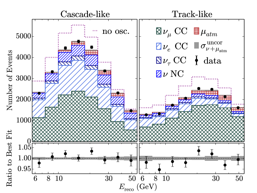
The $\nu_{\mu}$ CC reconstruction is used to estimate the direction and energy of the neutrino. The difference in best-fit likelihoods between the two hypotheses is used to classify our events as “track-like,” if inclusion of a muon track improves the fit substantially, or “cascade-like,” if the event is equally well fit without a muon. The reconstructed neutrino energy ( $E_{\text{reco}}$ ) distributions of events in each of these categories after final selection are shown in Fig. 1, along with the corresponding predicted distributions broken down by event type. The track-like sample is enriched in $\nu_{\mu}$ CC events (68% of sample), especially at higher energies where muons are more likely detected, while the cascade-like sample is evenly divided between $\nu_{\mu}$ CC and interactions without a muon in the final state. The angular and energy resolutions provided by the reconstruction are energy-dependent, with median resolutions of 10^∘ (16^∘) in zenith angle and 24% (29%) in neutrino energy for track-like (cascade-like) events at $E_{\nu}=20$ GeV.

Refer to caption — Figure 1: Reconstructed energy distributions observed in data (points) and predicted by interaction type at our best fit point for oscillations (stacked). In addition to each separate component, the uncorrelated statistical uncertainty associated to the expectation $\left(\sigma^{\text{uncor}}_{\nu+\mu_{\text{atm.}}}\right)$ is shown in a shaded band. The track-like sample is peaked at higher energy due to the rising probability of tagging $\nu_{\mu}$ CC events. The bottom plots show the ratio of the data to the fitted prediction.

The event selection in this analysis uses the DOMs surrounding the DeepCore region to veto atmospheric muons. The first criteria remove accidental triggers caused by dark noise by demanding a minimum amount of light detected in the DeepCore volume, with timing and spatial scale consistent with a particle emitting Cherenkov radiation. Events in which photons are observed outside the DeepCore volume before the light detected inside DeepCore, in a time window consistent with atmospheric muons penetrating to the fiducial volume, are then rejected. These are followed by a boosted decision tree (BDT) Hocker et al. (2007) which further reduces the background of atmospheric muons. The BDT uses the timing and spatial scale of the detected photoelectrons to select events with substantial charge deposition at the beginning of the event, indicative of a neutrino interaction vertex. It also considers how close the event is to the border of the DeepCore volume and the results of several fast directional reconstructions Ahrens et al. (2004) in determining whether the event may be an atmospheric muon. Finally, we demand that the interaction vertex reconstructed by the likelihood fit described above be contained within DeepCore and the end of the reconstructed muon be within the first row of DOMs outside DeepCore, which further reduces atmospheric muon contamination and improves reconstruction accuracy.

As these selection criteria reduce the atmospheric muon rate by a factor of approximately $10^{8}$ , it is challenging to simulate enough atmospheric muons to obtain a reliable prediction for the distribution of the remaining muons, especially in the presence of systematic uncertainties. We instead use a data-driven estimate of the shape of the muon background distributions, with the normalization free to float. This approach is based on tagging events that would have been accepted except for a small number of photons detected in the veto region, similar to the procedure in Ref. Aartsen et al. (2015). The uncertainty in the background shape is estimated using two different criteria for tagging these events, and was compared to the currently available muon Monte Carlo. This uncertainty is added in quadrature to the statistical uncertainties in the tagged background event sample and the neutrino Monte Carlo, to provide the total uncorrelated statistical uncertainty $\left(\sigma^{\text{uncor}}_{\nu+\mu_{\text{atm.}}}\right)$ in the expected distribution shown in Fig. 1.

IV Analysis

The final fit of the data is done using an $8\times 8\times 2$ binned histogram, with 8 bins in $\log_{10}{{E}_{\text{reco}}}$ , 8 bins in the cosine of the reconstructed neutrino zenith direction ( $\cos{\theta_{z,\text{reco}}}$ ), one track-like bin and one cascade-like. The bins are equally spaced with $\cos{\theta_{z,\text{reco}}}\in[-1,1]$ and $\log_{10}{E_{\text{reco}}}\in[0.75,1.75]$ . The fit assumes three-flavor oscillations with $\Delta m^{2}_{21}=7.53\times 10^{-5}$ eV², $\sin^{2}\theta_{12}=0.304$ , $\sin^{2}\theta_{13}=2.17\times 10^{-2}$ , and $\delta_{CP}=0^{\circ}$ .

We use MINUIT2 James and Roos (1975) to minimize a function

\chi^{2}=\sum_{i\in\{\text{bins}\}}\frac{(n^{\nu+\mu_{\text{atm}}}_{i}-n^{\text{data}}_{i})^{2}}{(\sigma^{\text{data}}_{i})^{2}+(\sigma^{\text{uncor}}_{\nu+\mu_{\text{atm}},i})^{2}}+\sum_{j\in\{\text{syst}\}}\frac{(s_{j}-\hat{s}_{j})^{2}}{\hat{\sigma}_{s_{j}}^{2}},

(2)

where $n^{\nu+\mu_{\text{atm}}}_{i}$ is the number of events expected in the $i^{th}$ bin, which is the sum of neutrino events weighted to the desired oscillation parameters using Prob3++ Wendell et al. and the atmospheric muon background. The number of events observed in the $i^{th}$ bin is $n^{\text{data}}_{i}$ , with Poisson uncertainty $\sigma^{\text{data}}_{i}=\sqrt{n^{\text{data}}_{i}}$ , and $\sigma^{\text{uncor}}_{\nu+\mu_{\text{atm}},i}$ is the uncertainty in the prediction of the number of events of the $i^{th}$ bin. $\sigma^{\text{uncor}}_{\nu+\mu_{\text{atm}}}$ includes both effects of finite MC statistics and uncertainties in our data-driven muon background estimate. The second term of Eq. (2) is a penalty term for our nuisance parameters, where $s_{j}$ is the value of $j^{th}$ systematic, $\hat{s}_{j}$ is the central value and $\hat{\sigma}_{s_{j}}^{2}$ is the Gaussian width of the $j^{th}$ systematic prior.

The analysis includes eleven nuisance parameters describing our systematic uncertainties, summarized in Table 1. Seven of these are related to systematic uncertainties in the atmospheric neutrino flux and interaction cross sections. Since only the event rate is observed directly, some uncertainties in flux and cross section have similar effects on the data. In these cases, the degenerate effects are combined into a single parameter. Because analytical models of these effects are available, these parameters can be varied continuously by reweighting simulated events.

The first nuisance parameter is the overall normalization of the event rate. It is affected by uncertainties in the atmospheric neutrino flux and the neutrino interaction cross section, and by the possibility of accidentally vetoing neutrino events due to unrelated atmospheric muons detected in the veto volume. This last effect is expected to reduce the neutrino rate by several percent, but is not included in the present simulations. Because of this and the fact it encompasses several effects, no prior is used for this parameter.

A second parameter allows an energy-dependent shift in the event rate. This can arise from uncertainties in either the spectral index of the atmospheric flux (nominally $\gamma=-2.66$ at the relevant energies in our neutrino flux model Honda et al. (2015)), or the deep inelastic scattering (DIS) cross section. A prior of $\hat{\sigma}_{s}=0.10$ is placed on the spectral index to describe the range of these uncertainties.

Several uncertainties on the DIS cross section were implemented in the fit, but found either to have negligible impact or to be highly degenerate with the normalization and spectral index parameters over the energy range of this analysis. These include variation of parameters of the Bodek-Yang model Bodek and Yang (2003) used in GENIE, uncertainties in the differential DIS cross-section, and hadronization uncertainties for high- $W$ DIS events Katori et al. (2016). As these effects are captured by the first two nuisance parameters, the additional parameters were not used.

One neutrino cross-section uncertainty was not well described by these parameters: the uncertainty of the axial mass form factor for resonant events. The default value of 1.12 GeV and prior of 0.22 GeV were taken from GENIE Andreopoulos et al. (2010). Uncertainties in CCQE interactions were also investigated but had no impact on the analysis due to the small percentage of CCQE events at these energies.

The normalizations of $\nu_{e}+\bar{\nu}_{e}$ events and NC events, defined relative to $\nu_{\mu}+\bar{\nu}_{\mu}$ CC events, are both assigned an uncertainty of 20%. Uncertainties in hadron production (especially pions and kaons) in air showers affect the predicted flux, in particular the ratio of neutrinos to anti-neutrinos. We model these hadronic flux effects with two parameters, one dependent on neutrino energy and the other on the zenith angle, chosen to reproduce the uncertainties estimated in Ref. Barr et al. (2006). Their total uncertainty varies from 3%-10% depending on the energy and zenith angle, so the fit result is given in units of $\sigma$ as calculated by Barr et al. Uncertainties in the relative cross section of neutrinos vs. anti-neutrinos are degenerate with the flux uncertainty in this energy range.

Table 1: Table of nuisance parameters along with their associated priors, if applicable. The right two columns show the results from our best fit for normal mass ordering and inverted mass ordering, respectively.

Flux and cross section parameters
Parameters	Priors	Best Fit
Parameters	Priors	NO	IO
Neutrino event rate [% of nominal]	no prior	85	85
$\Delta\gamma$ (spectral index)	0.00 $\pm$ 0.10	-0.02	-0.02
$M_{A}$ (resonance) [GeV]	1.12 $\pm$ 0.22	0.92	0.93
$\nu_{e}+\bar{\nu}_{e}$ relative normalization [%]	100 $\pm$ 20	125	125
NC relative normalization [%]	100 $\pm$ 20	106	106
Hadronic flux, energy dependent [ $\sigma$ ]	0.00 $\pm$ 1.00	-0.56	-0.59
Hadronic flux, zenith dependent [ $\sigma$ ]	0.00 $\pm$ 1.00	-0.55	-0.57
Detector parameters
overall optical eff. [%]	100 $\pm$ 10	102	102
relative optical eff., lateral [ $\sigma$ ]	0.0 $\pm$ 1.0	0.2	0.2
relative optical eff., head-on [a.u.]	no prior	-0.72	-0.66
Background
Atm. $\mu$ contamination [% of sample]	no prior	5.5	5.6

Systematics related to the response of the detector itself, including photon propagation through the ice and the anisotropic sensitivity of the DOMs, have the largest impact on this analysis. Their effects are estimated by Monte Carlo simulation at discrete values, with the contents of each bin in the (energy, direction, track/cascade) analysis histogram determined by linear interpolation between the discrete simulated models, following the approach of Ref. Aartsen et al. (2015, 2017a).

Uncertainties in the efficiency of photon detection are driven by the formation of bubbles in the refrozen ice columns in the holes where the IceCube strings were deployed. A prior with a width of 10% was applied to the overall photon collection efficiency Aartsen et al. (2017b), parametrized using seven MC data sets ranging from 88% to 112% of the nominal optical efficiency. In addition to modifying the absolute efficiency, these bubbles can scatter Cherenkov photons near the DOMs, modulating the relative optical efficiency as function of the incident photon angle. The effect of the refrozen ice column is modeled by two effective parameters controlling the shape of the DOM angular acceptance curve.

The first parameter controls the lateral angular acceptance (i.e., relative sensitivity to photons traveling roughly 20^∘ above versus below the horizontal) and is fairly well constrained by LED calibration data. Five MC data sets were generated covering the $-1\sigma$ to $+1\sigma$ uncertainty from the LED calibration, and parametrized in the same way as the overall optical efficiency described above. A Gaussian prior based on the LED data is used.

The second parameter controls sensitivity to photons traveling vertically upward and striking the DOMs head-on, which is not well constrained by string-to-string LED calibration. That effect is modeled using a dimensionless parameter ranging from -5 (corresponding to a bubble column completely obscuring the DOM face for vertically incident photons) to $2.5$ (no obscuration). Zero corresponds to constant sensitivity for angles of incidence from $0^{\circ}$ to $30^{\circ}$ from vertical. Six MC sets covering the range from -5 to 2 were used to parametrize this effect. No prior is applied to this parameter due to lack of information from calibration data.

The last nuisance parameter controls the level of atmospheric muon contamination in the final sample. As described above, the shape of this background in the analysis histogram, including binwise uncertainties, is derived from data. Since the absolute efficiency for tagging background events with this method is unknown, the normalization of the muon contribution is left free in the fit.

In addition to the systematic uncertainties discussed above, we have considered the impact of seed dependence in our event reconstruction, different optical models for both the undisturbed ice and the refrozen ice columns, and an improved detector calibration currently being prepared. In all these cases the impact on the final result was found to be minor, and they were thus omitted from the fit and the error estimate.

V Results and Conclusion

The analysis procedure described above gives a best fit of $\Delta m^{2}_{32}=2.31^{+0.11}_{-0.13}\times 10^{-3}$ eV² and $\sin^{2}\theta_{23}=0.51^{+0.07}_{-0.09}$ , assuming normal neutrino mass ordering (NO). For the inverted mass ordering (IO), the best fit shifts to $\Delta m^{2}_{32}=-2.32\times 10^{-3}$ eV² and $\sin^{2}\theta_{23}=0.51$ . The pulls on the nuisance parameters are shown in Table 1. Though IceCube’s current sensitivity to the mass ordering is low, dedicated analyses are underway to measure this.

The data agree well with the best-fit MC data set, with $\chi^{2}=117.4$ for both neutrino mass orderings. This corresponds to a $p$ -value of 0.52 given the 119 effective degrees of freedom estimated via toy MCs, following the procedure described in Ref. Aartsen et al. (2017a).

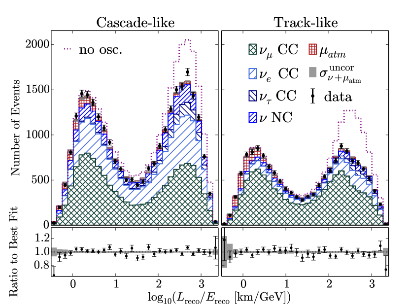
To better visualize the fit, Fig. 2 shows the results of the fit projected onto a single $L/E$ axis, for both the track-like and cascade-like events. The two peaks in each distribution correspond to down-going and up-going neutrino trajectories. Up-going $\nu_{\mu}+\bar{\nu}_{\mu}$ are strongly suppressed in the track-like channel due to oscillations. Some suppression of up-going cascade-like data is also visible, due to disappearance of lower-energy $\nu_{\mu}$ which are not tagged as track-like by our reconstruction.

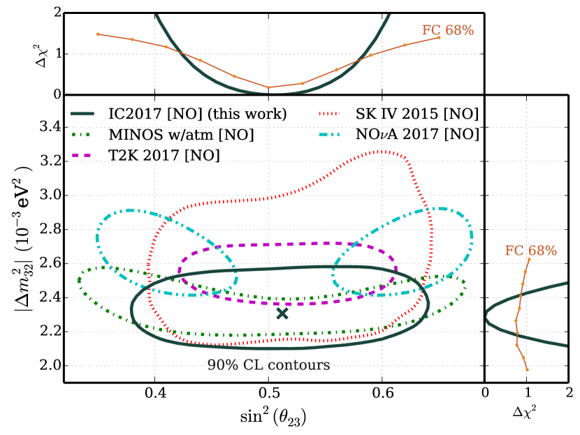
Figure 3 shows the region of $\sin^{2}\theta_{23}$ and $\Delta m^{2}_{32}$ allowed by our analysis at 90% C.L., along with our best fit and several other leading measurements of these parameters Abe et al. (2017); Wendell (2015); Adamson et al. (2013, 2017). The contours are calculated using the approach of Feldman and Cousins Feldman and Cousins (1998) to ensure proper coverage.

Our results are consistent with those from other experiments Abe et al. (2017); Wendell (2015); Adamson et al. (2013, 2017); An et al. (2017), but using significantly higher energy neutrinos and subject to a different set of systematic uncertainties. Our data prefer maximal mixing, similar to the result from T2K Abe et al. (2017). The best-fit values from the NO $\nu$ A experiment Adamson et al. (2017) are disfavored by $\Delta\chi^{2}=8.9$ (first octant) or $\Delta\chi^{2}=8.8$ (second octant), corresponding to a significance of $2.6\sigma$ using the method of Feldman and Cousins, although there is considerable overlap in the 90% confidence regions of the two measurements. Further improvements to our analysis are underway, including the incorporation of additional years of data, extensions of our event selections, and improved calibration of the detector response.

Acknowledgements

Acknowledgements.

We acknowledge the support from the following agencies: U.S. National Science Foundation-Office of Polar Programs, U.S. National Science Foundation-Physics Division, University of Wisconsin Alumni Research Foundation, Michigan State University, the Grid Laboratory Of Wisconsin (GLOW) grid infrastructure at the University of Wisconsin - Madison, the Open Science Grid (OSG) grid infrastructure; U.S. Department of Energy, and National Energy Research Scientific Computing Center, the Louisiana Optical Network Initiative (LONI) grid computing resources; Natural Sciences and Engineering Research Council of Canada, WestGrid and Compute/Calcul Canada; Swedish Research Council, Swedish Polar Research Secretariat, Swedish National Infrastructure for Computing (SNIC), and Knut and Alice Wallenberg Foundation, Sweden; German Ministry for Education and Research (BMBF), Deutsche Forschungsgemeinschaft (DFG), Helmholtz Alliance for Astroparticle Physics (HAP), Initiative and Networking Fund of the Helmholtz Association, Germany; Fund for Scientific Research (FNRS-FWO), FWO Odysseus programme, Flanders Institute to encourage scientific and technological research in industry (IWT), Belgian Federal Science Policy Office (Belspo); Marsden Fund, New Zealand; Australian Research Council; Japan Society for Promotion of Science (JSPS); the Swiss National Science Foundation (SNSF), Switzerland; National Research Foundation of Korea (NRF); Villum Fonden, Danish National Research Foundation (DNRF), Denmark

References

Fukuda et al. (1998) Y. Fukuda et al. (Super-Kamiokande), Phys. Rev. Lett. 81, 1562 (1998), eprint hep-ex/9807003.
Ahmad et al. (2001) Q. R. Ahmad et al. (SNO), Phys. Rev. Lett. 87, 071301 (2001), eprint nucl-ex/0106015.
Pontecorvo (1957) B. Pontecorvo, Sov. Phys. JETP 6, 429 (1957), [Zh. Eksp. Teor. Fiz.33,549(1957)].
Maki et al. (1962) Z. Maki, M. Nakagawa, and S. Sakata, Prog. Theor. Phys. 28, 870 (1962).
Volkova (1980) L. V. Volkova, Sov. J. Nucl. Phys. 31, 784 (1980), [Yad. Fiz.31,1510(1980)].
Barr et al. (2004) G. D. Barr, T. K. Gaisser, P. Lipari, S. Robbins, and T. Stanev, Phys. Rev. D70, 023006 (2004), eprint astro-ph/0403630.
Honda et al. (2015) M. Honda, M. S. Athar, T. Kajita, K. Kasahara, and S. Midorikawa, Phys. Rev. D92, 023004 (2015), eprint 1502.03916.
Wolfenstein (1978) L. Wolfenstein, Phys. Rev. D17, 2369 (1978).
Petcov (1998) S. T. Petcov, Phys. Lett. B434, 321 (1998), eprint hep-ph/9805262.
Akhmedov et al. (2007) E. K. Akhmedov, M. Maltoni, and A. Yu. Smirnov, JHEP 05, 077 (2007), eprint hep-ph/0612285.
Akhmedov et al. (2008) E. K. Akhmedov, M. Maltoni, and A. Yu. Smirnov, JHEP 06, 072 (2008), eprint 0804.1466.
Adamson et al. (2013) P. Adamson et al. (MINOS), Phys. Rev. Lett. 110, 251801 (2013), eprint 1304.6335.
Abe et al. (2017) K. Abe et al. (T2K), Phys. Rev. Lett. 118, 151801 (2017), eprint 1701.00432.
Adamson et al. (2017) P. Adamson et al. (NOvA), Phys. Rev. Lett. 118, 151802 (2017), eprint 1701.05891.
An et al. (2017) F. P. An et al. (Daya Bay), Phys. Rev. D95, 072006 (2017), eprint 1610.04802.
Wendell (2015) R. Wendell (Super-Kamiokande), AIP Conf. Proc. 1666, 100001 (2015), eprint 1412.5234.
Formaggio and Zeller (2012) J. A. Formaggio and G. P. Zeller, Rev. Mod. Phys. 84, 1307 (2012), eprint 1305.7513.
Friedland et al. (2004) A. Friedland, C. Lunardini, and M. Maltoni, Phys. Rev. D70, 111301 (2004), eprint hep-ph/0408264.
Friedland and Lunardini (2005) A. Friedland and C. Lunardini, Phys. Rev. D72, 053009 (2005), eprint hep-ph/0506143.
Ohlsson et al. (2013) T. Ohlsson, H. Zhang, and S. Zhou, Phys. Rev. D88, 013001 (2013), eprint 1303.6130.
Esmaili and Smirnov (2013) A. Esmaili and A. Yu. Smirnov, JHEP 06, 026 (2013), eprint 1304.1042.
Gonzalez-Garcia and Maltoni (2013) M. C. Gonzalez-Garcia and M. Maltoni, JHEP 09, 152 (2013), eprint 1307.3092.
Mocioiu and Wright (2015) I. Mocioiu and W. Wright, Nucl. Phys. B893, 376 (2015), eprint 1410.6193.
Choubey and Ohlsson (2014) S. Choubey and T. Ohlsson, Phys. Lett. B739, 357 (2014), eprint 1410.0410.
Coloma and Schwetz (2016) P. Coloma and T. Schwetz, Phys. Rev. D94, 055005 (2016), [Erratum: Phys. Rev. D95, 079903 (2017)], eprint 1604.05772.
Liao et al. (2016) J. Liao, D. Marfatia, and K. Whisnant, Phys. Rev. D93, 093016 (2016), eprint 1601.00927.
Aartsen et al. (2017a) M. G. Aartsen et al. (IceCube), Phys. Rev. D95, 112002 (2017a), eprint 1702.05160.
Aartsen et al. (2015) M. G. Aartsen et al. (IceCube), Phys. Rev. D91, 072004 (2015), eprint 1410.7227.
Aartsen et al. (2017b) M. G. Aartsen et al. (IceCube), JINST 12, P03012 (2017b), eprint 1612.05093.
Abbasi et al. (2009) R. Abbasi et al. (IceCube), Nucl. Instrum. Meth. A601, 294 (2009), eprint 0810.4930.
Abbasi et al. (2010) R. Abbasi et al. (IceCube), Nucl. Instrum. Meth. A618, 139 (2010), eprint 1002.2442.
Abbasi et al. (2012) R. Abbasi et al. (IceCube), Astropart. Phys. 35, 615 (2012), eprint 1109.6096.
Andreopoulos et al. (2010) C. Andreopoulos et al., Nucl. Instrum. Meth. A614, 87 (2010), eprint 0905.2517.
Agostinelli et al. (2003) S. Agostinelli et al. (GEANT4), Nucl. Instrum. Meth. A506, 250 (2003).
Radel and Wiebusch (2012) L. Radel and C. Wiebusch, Astropart. Phys. 38, 53 (2012), eprint 1206.5530.
Koehne et al. (2013) J. H. Koehne, K. Frantzen, M. Schmitz, T. Fuchs, W. Rhode, D. Chirkin, and J. Becker Tjus, Comput. Phys. Commun. 184, 2070 (2013).
(37) C. Kopper et al., https://github.com/claudiok/clsim.
Aartsen et al. (2013) M. G. Aartsen et al. (IceCube), Nucl. Instrum. Meth. A711, 73 (2013), eprint 1301.5361.
Feroz et al. (2009) F. Feroz, M. P. Hobson, and M. Bridges, Mon. Not. Roy. Astron. Soc. 398, 1601 (2009), eprint 0809.3437.
Hocker et al. (2007) A. Hocker et al., PoS ACAT, 040 (2007), eprint physics/0703039.
Ahrens et al. (2004) J. Ahrens et al. (AMANDA), Nucl. Instrum. Meth. A524, 169 (2004), eprint astro-ph/0407044.
James and Roos (1975) F. James and M. Roos, Comput. Phys. Commun. 10, 343 (1975).
(43) R. Wendell et al., http://www.phy.duke.edu/~raw22/public/Prob3++.
Bodek and Yang (2003) A. Bodek and U. K. Yang, J. Phys. G29, 1899 (2003), eprint hep-ex/0210024.
Katori et al. (2016) T. Katori, P. Lasorak, S. Mandalia, and R. Terri, JPS Conf. Proc. 12, 010033 (2016), eprint 1602.00083.
Barr et al. (2006) G. D. Barr, S. Robbins, T. K. Gaisser, and T. Stanev, Phys. Rev. D74, 094009 (2006), eprint astro-ph/0611266.
Feldman and Cousins (1998) G. J. Feldman and R. D. Cousins, Phys. Rev. D57, 3873 (1998), eprint physics/9711021.

VI Supplemental Material

Control of systematic uncertainties in this analysis relies fundamentally on the use of the full 3D space of neutrino energy, arrival direction (correlated with path length through the Earth), and particle type to disentangle systematic uncertainties from the neutrino oscillation physics of interest. Oscillation effects have a distinctive shape in the $L/E_{\nu}$ space and primarily affect $\nu_{\mu}$ CC events, while systematic effects have a much broader impact on the data. A complete description of our methodology will be included in a more detailed forthcoming paper which extends this analysis to measure the rate of $\nu_{\tau}$ appearance. In this supplement, we provide an abbreviated discussion to illustrate the approach.

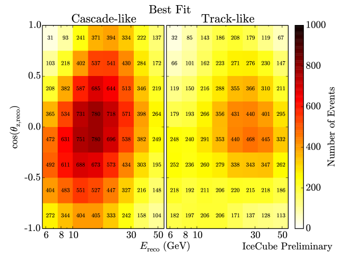
This analysis divides the data into 128 bins in three dimensions: eight bins in $\log_{10}(E_{\nu,\mathrm{reco}})$ , eight bins in $\cos({\theta_{z,reco}})$ , and two bins for particle identification, track-like and cascade-like. Ideally, $\nu_{\mu}$ CC events are classified as track-like while $\nu_{e}$ $\nu_{\tau}$ , and NC events should be classified as cascade-like; in practice there is leakage between the samples due to imperfect particle identification. In our letter, we provide projections of the underlying data so that the oscillatory behavior in reconstructed $L/E_{\nu}$ and the energy range of the data set may be seen clearly. The full 3D distribution of the data is shown in Fig. S1.

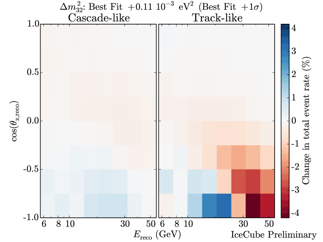
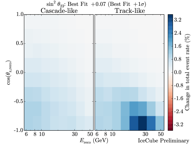
Oscillations affect upward-going $\nu_{\mu}$ CC events, which are enriched in the track-like sample but also contribute to the cascade-like sample (especially at lower reconstructed energy). Downward-going neutrinos with baselines too short for oscillations to occur and cascade-like events provide constraints on systematic uncertainties related to the atmospheric flux, neutrino interactions, and detector response. Our measurement of the oscillation parameters is obtained mainly from the higher energy bins, as shown in Figs. S2 and S3, due to the improved angular and energy resolution and particle identification accuracy we obtain at higher energies. These figures shows how the $\chi^{2}$ sum would change if the values of $\Delta m^{2}_{32}$ and $\sin^{2}(\theta_{23})$ were increased by $1\sigma$ from their best-fit values. The relative effects on the event rate itself are shown in Figs. S4 and S5. Note that while a number of $\nu_{\mu}$ CC events are incorrectly reconstructed as cascade-like, as shown in Fig. 2 of the letter, their impact on the measurement of the oscillation parameters is relatively small compared to the high-energy track-like sample.

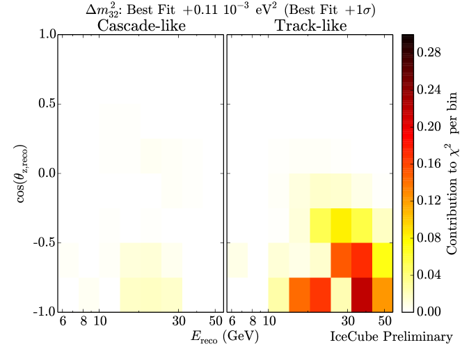
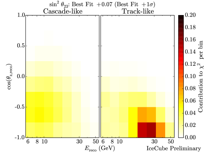
The patterns shown in Figs. S2 and S3 are the oscillation signature that must be distinguished from the effects of systematics. There are eleven different systematic uncertainties implemented in this analysis, each with their own distinctive signature. Crucially, all of these effects have a much broader impact on the data set than the oscillation physics – large numbers of bins in both the cascade-like and track-like samples are affected.

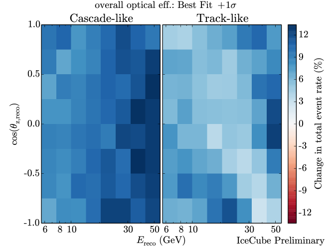
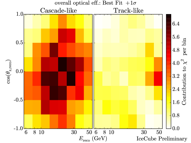
As an example, the impact of a shift in the overall optical efficiency of the DOMs, and the range of bins which constrain this effect, are shown in Figs. S6 and S7. The figure shows how a 10% increase in collection efficiency for Cherenkov photons (the width of the a priori uncertainty in this parameter) would affect the event distribution, with all other parameters held fixed. If only upward-going track-like events in the 10–40 GeV range were considered, there would be strong correlation with $\sin^{2}(\theta_{23})$ : higher optical efficiency produces an increase in the event rate, which partly fills in the disappearance minimum. However, the effect of varying optical efficiency extends throughout both the cascade-like and track-like distributions, affecting both upward-going and downward-going events at all energies, while the effect of oscillations is well localized to the 10–40 GeV range at angles of $\cos(\theta_{z,\textrm{reco}})<-0.6$ , as shown in Fig. S5. Consideration of the full energy vs. angle distribution of both samples thus allows the two effects to be disentangled effectively. As shown in Fig. S7, the constraint on this systematic arises almost entirely from the cascade sample. Due to the correlations with oscillation parameters, the fitter does not obtain constraints on this systematic from up-going high-energy $\nu_{\mu}$ tracks.

Affecting the measurement of $\Delta m^{2}_{32}$ is particularly complicated, since it requires shifting the position of the oscillation dip. Such a shift requires both increases and decreases in event rate in neighboring bins, while leaving most of the distribution unaffected, as shown in Fig. S4. This complexity permits relatively tight constraints on that parameter. The optical efficiency of the DOMs is the leading contributor to the uncertainty budget for this parameter, and in fact is the systematic which is most closely correlated individually with the oscillation parameters (see Fig. S8 below), but even so, perfect knowledge of the optical efficiency would only improve the precision of the measurement of this parameter by about 20% given current angular and energy resolutions and current knowledge of other systematic effects.

In practice, all eleven systematic uncertainties and both oscillation parameters are fitted simultaneously. The optimization routine explores all possible combinations of systematics that could mimic the more tightly localized effect of oscillation physics at specific ranges of energy and zenith angle. The correlation matrix shown in Fig. S8 illustrates the correlations between the systematic parameters and the oscillation parameters. While some of the systematics are correlated with each other, the wide ranges of baselines and energies over which we observe neutrinos enable us to disentangle these effects from the distortions of the observed atmospheric neutrino flux produced by neutrino oscillations.