Atomic physics and modern solar spectro-polarimetry

Abstract

Observational solar physics is entering a new era with the advent of new 1.5 m class telescopes with adaptive optics, as well as the Daniel K. Inouye 4 m telescope which will become operational in 2019. Major outstanding problems in solar physics all relate to the solar magnetic field. Spectropolarimetry offers the best, and sometimes only, method for accurate measurements of the magnetic field. In this paper we highlight how certain atomic transitions can help us provide both calibration data, as well as diagnostic information on solar magnetic fields, in the presence of residual image distortions through the atmosphere close to, but not at the diffraction limits of large and polarizing telescopes. Particularly useful are spectral lines of neutrals and singly charged ions of iron and other complex atoms. As a proof-of-concept, we explore atomic transitions that might be used to study magnetic fields without the need for an explicit calibration sequence, offering practical solutions to the difficult challenges of calibrating the next generation of solar spectropolarimetric telescopes. Suggestions for additional work on atomic theory and measurements, particularly at infrared wavelengths, are given. There is some promise for continued symbiotic advances between solar physics and atomic physics.

1. Introduction

The fields of solar and atomic physics have enjoyed decades of fruitful collaborations (e.g. Gabriel and Jordan, 1971; Dufton and Kingston, 1981). The Sun is our best “laboratory” for studying the behavior of an archetypal, nearly-ideal plasma under conditions of very high magnetic Reynolds numbers (e.g. Parker, 1979). The Sun also spans wide ranges of plasma $\beta=8\pi P/B^{\mathrm{2}}$. On average, $\beta\gg 1$ in the interior, $\beta\approx 1$ in the atmosphere (from which the bulk of the solar radiation escapes), and $\ll 1$ in the solar corona.

The Sun exhibits complex behavior, i.e. patterns emerge from non-linear governing equations of motion, a result that appears larger than the sum of the parts. Yet, seven decades after the development of magneto-hydro-dynamics, the simplest model capable of entertaining such behavior, we still are unable to answer the deceptively simple question: How does the Sun regulate its strikingly ordered and ever-changing magnetic field?.

Solar differential rotation, in spite of (or perhaps because of) turbulent convection beneath the solar surface, leads to well-known patterns of magnetic structure, such as the remarkable “sunspot cycle”. Every eleven years the entire global solar magnetic field reverses. This occurs in a system in which the global magnetic diffusion time is some $10^{\mathrm{9}}$ years. We also do not know the physical reasons why the Sun is obliged to form spots. These intense concentrations of magnetic field, too often taken for granted, were first studied in Galileo’s era. But why does magnetic flux appear in such intense concentrations in the Sun, sometimes exceeding field strengths in equipartition with the convection?

Table 1Regimes of spectral line polarization in solar plasmas

	Ion	Multi-	$|{\bf B}|$	$\omega_{\mathrm{L}}$	$\omega_{\mathrm{Dopp}}$	$2\pi A$	$\epsilon_{\mathrm{Z}}$	$\epsilon_{\mathrm{H}}$
	charge	pole	G	[rad/s]	[rad/s]	[rad/s]	$=\omega_{\mathrm{L}}/\omega_{\mathrm{Dopp}}$	$=\omega_{\mathrm{L}}/2\pi A$
photosphere	0,1	E1	$10..3(3)$	$1(8)..3({10})$	$4({10})$	$5(8)$	$2({-3})..1$	$0.2..60$
chromosphere	0,1	E1	$10..1(3)$	$1(8)..1({10})$	$4({10})$	$5(8)$	$2({-3})..0.4$	$0.2..20$
corona	$7..14$	M1	$1..100$	$1(7)..1(9)$	$4({11})$	50	$2({-5})..2({-2})$	$2(5)..2(7)$
prominence/filament	0,1	E1	$5..50$	$7(7)..7(8)$	$4({10})$	$5(8)$	$2({-3})..2({-2})$	$0.14..1.4$

The table shows data for the photosphere, chromosphere, corona and prominences. The lower field strength regions apply to quiet regions, the higher values to the strongest concentrations (the darkest regions of sun spots). Typical values are listed for the Larmor frequency of atoms and ions ($\omega_{\mathrm{L}}$), the Doppler width ($\omega_{\mathrm{Dopp}}$) and natural width ($2\pi A$) of the lines in angular frequency units, and the ratios of these parameters. A reference wavelength of $\lambda=$5000 Å was adopted in making this table, the values of $\omega_{\mathrm{Dopp}}$ vary as $\lambda^{\mathrm{-1}}$. The notation $X(Y)$ means $X\times 10^{\mathrm{Y}}$. When $\epsilon_{\mathrm{Z}}\ll 1$ the Zeeman intensity profiles are unsplit, broadened, and the induced polarization is small. When $0.1<\epsilon_{\mathrm{H}}<100$ the Hanle effect is important.

Such are the nature of some of the major unsolved problems in solar physics.

2. The continuing need for observations

Following decades of exponential advances in computations, it might be surprising that numerical experiments are far from providing us with an ab-initio understanding of the Sun’s behavior. However, this is because of the extreme range of scales involved. Consider the governing equation for the magnetic field in magneto-hydrodynamics, readily derived from Faraday’s Law of Electromagnetic Induction and Ohm’s Law (kinetic collisional dynamics):

$${{\partial{\bf B}}\over{\partial t}}={\bf curl\,}({\bf u}\times{\bf B})+\eta\nabla^{\mathrm{2}}{\bf B},$$ (1)

where, in the solar interior for example, the magnetic diffusivity $\eta$ is $\approx$ $10^{\mathrm{4}}$ cm²s^-1. Over scales of a fraction of a solar radius $\ell\approx 10^{\mathrm{10}}$ cm, ordered flows are $\approx 0.1$  km s^-1. Thus the “magnetic Reynolds number” is $|{\bf u}|\ell/\eta\approx 10^{\mathrm{10}}$. 3D numerical simulations typically have $R_{\mathrm{M}}\mathrel{\hbox to0.0pt{\lower 3.7pt\hbox{$\sim$} \hss}\raise 1.7pt\hbox{$<$}}10^{\mathrm{4}}$. The numerical range of scales is some 6 orders of magnitude smaller than the physical range. The Lorentz force, $({\bf curl\,}{\bf B})\times{\bf B}$, increases with inverse scale length, not allowing us to invoke a “simple” turbulent cascade (Parker, 2009). Therefore, the fundamental physics of magnetic regeneration – the “dynamo” problem – implies that

solar physics remains an observationally-driven science.

To measure magnetic fields, spectropolarimetry, developed from the 1960s, is the most powerful tool at hand. With the advent of new 1.5-meter to 4-meter class telescopes, spectropolarimetry is poised to make important breakthroughs. These new telescope systems off higher angular resolution, larger photon flux, access to thermal infrared regions and coronagraphic capabilities. With modern adaptive optics systems (Rimmele and Marino, 2011), these instruments will permit us to study evolving surface magnetic fields across the physical scales of interest.

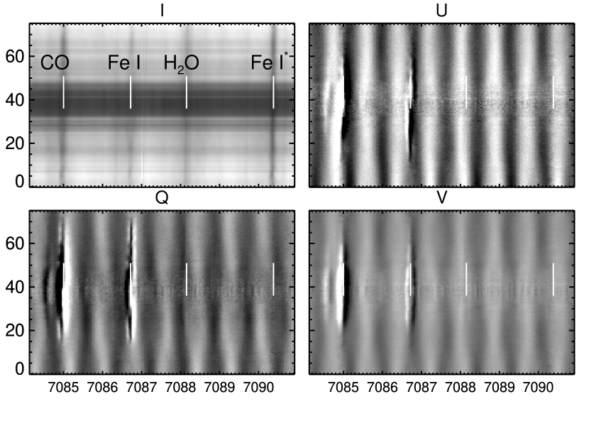
Figure 1.— Minimally processed Stokes spectra are shown for the 709.0 nm region, obtained 21st August 2014 at the Dunn Solar Telescope using the SPINOR spectro-polarimeter. Standard calibration procedures were applied with no attempts to ”massage” these data. The abscissa is wavelength in Å, the ordinate position along the spectrograph slit (arc seconds). The middle dark portion is the umbra (darkest region) of a small sunspot in NOAA active region 12147. The 709.04 nm transition of Fe I (${\rm 5s\,^{\mathrm{5}}F_{\mathrm{1}}\rightarrow 4p\,^{\mathrm{5}}D^{\mathrm{O}}_{\mathrm{0}}}$, both with the ${\rm 3p^{\mathrm{6}}3d^{\mathrm{7}}(^{\mathrm{4}}F)}$ core), shows zero polarization at the sensitivity levels achieved in these observations. The $Q,U$ panels are color scaled between $\pm 0.02I$, $V$ is shown between $\pm 0.1I$.

Observations and and numerical experiments yield “effective” (i.e. non-kinetic, or “turbulent”) diffusivities of $\approx 10^{\mathrm{12}}$ cm²s^-1 (e.g. Berger et al., 1998; Cameron et al., 2011), sufficient to account for the 11 year evolution time of the solar magnetic field. But these diffusivities as yet have no solid justification in physics (Parker, 2009). But if we accept these values, with convective speeds $u$ of order 3  km s^-1, this diffusion coefficient $\eta\approx\frac{1}{3}u\ell$ implies $\ell\approx 100$ km. The 4-meter Daniel K. Inouye Solar Telescope (DKIST, previously ATST, Keil et al., 2009) will resolve scales down to $\approx 20$ km. New DKIST observations will therefore help us answer the most pressing questions regarding the evolution of solar magnetism.

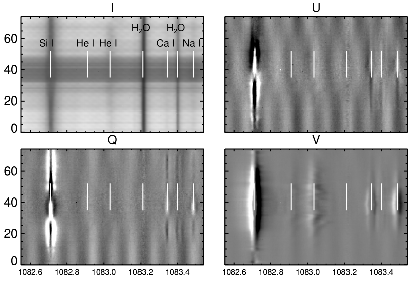
Figure 2.— Simultaneous SPINOR spectra as in 1 for the region near the 1083 nm multiplet of He I. All solar lines show polarization signals, there is also a signal from the telluric (unpolarized) line of H₂O (see the panel for Stokes $Q,U$ only near 1083.4 nm and $y=$) which must be due to an inaccurate polarization calibration. Notice that, unlike the 709 nm region shown in Figure 1, the $QUV$ profiles (e.g., of Si I 1082.7 nm) are consistent with solar Zeeman patterns, the polarization calibration is easier at infrared wavelengths.

Before proceeding, we display some data in figures 1 and 2. They show Stokes (polarized) spectra. In natural sources like the Sun, polarized light occurs through averages of incoherent packets of photons. In solar work it is therefore traditional to use the Stokes parameters $(I,Q,U,V)^{\mathrm{T}}$ written as an array ${\bf S}$, which can be simply related to the coherency matrix. Here $I$ is the intensity, $Q,U$ are the linear polarization parameters, $V$ circular. It is possible to give an operational definition of ${\bf S}$ in terms of an ideal linear polarizer and retarder set at different angles relative to a fixed direction in the plane of polarization (see, e.g., Landi Degl’Innocenti and Landolfi, 2004, ch. 1).

The data shown were taken with the SPINOR instrument at the Dunn Solar Telescope (DST), which in these data has an angular resolution of $\approx 400$ km at the solar surface. The DST is fed by a plane heliostat and the optical system is far from symmetric (with consequences discussed more below). These data were obtained simultaneously under typical observing conditions at red and infrared wavelengths using a state-of-the-art adaptive optics system. They show several properties: real solar signals, “cross-talk” from $V$ to $Q$ and $U$ (the 709 nm region has lines with non-physical antisymmetric $Q,U$ profiles), optical fringing, at the level of 1%, and some unphysical polarization in telluric (H₂O) lines. The non-solar signals are the main concern of this article. Several ways in which the modern telescopes in fact make polarimetry more challenging are discussed below.

3. New regimes for spectro-polarimetry

Remarkably, the Sun is simply not bright enough to tackle the demands of measurements of solar magnetism (Landi Degl’Innocenti, 2013). Solar fields are weak compared with laboratory fields, and Zeeman splittings are small compared to Doppler widths (i.e. $\epsilon_{\mathrm{Z}}\ll 1$ in Table 1). Information on the magnetic field is therefore encoded mostly through spectral line polarization, the Zeeman splitting in intensity profiles being far smaller than the line widths.

The Sun’s visible ($\lambda\approx$ 5000 Å) intensity is $I_{\mathrm{\lambda}}\approx B_{\mathrm{\lambda}}(T$=5500K) erg cm^-2 s^-1 sr^-1Å^-1, where $B_{\mathrm{\lambda}}$ is the Planck function. To compute the photon flux density from a solar area subtending a solid angle of $\varpi$ steradians, we have $f_{\mathrm{\lambda}}=\varpi B_{\mathrm{\lambda}}(\lambda/hc)$ photons cm^-2Å^-1s^-1. For a telescope of diameter $D$ cm, the flux from this area, integrated over the aperture is

$$F_{\mathrm{\lambda}}=\varpi B_{\mathrm{\lambda}}\frac{\lambda}{hc}\frac{\pi D^{\mathrm{2}}}{4}{\rm photons~{}\AA{}^{\mathrm{-1}}~{}s^{\mathrm{-1}}}.$$ (2)

If we critically sample the solar image spatially at the diffraction limit, i.e. at half of the diameter of the telescope point spread function, then $\varpi=\left(1.22\lambda/2D\right)^{\mathrm{2}}$, and

$$F_{\mathrm{\lambda}}^{\mathrm{DL}}=\frac{\pi}{4}B_{\mathrm{\lambda}}\frac{\lambda}{hc}\frac{(1.22\lambda)^{\mathrm{2}}}{4}=3.8\times 10^{\mathrm{8}}\ {\rm photons~{}\AA{}^{\mathrm{-1}}~{}s^{\mathrm{-1}}},$$ (3)

independent of the telescope aperture. Photospheric Doppler widths are 2-3  km s^-1. Spectrographs with resolutions $R\mathrel{\hbox to0.0pt{\lower 3.7pt\hbox{$\sim$} \hss}\raise 1.7pt\hbox{$>$}}200,000$ ($\equiv 1.5$  km s^-1, $\equiv 0.024$ Å @ 5000 Å) are typically used. But Zeeman-induced polarization is of order $\epsilon_{\mathrm{Z}}{dI}/{d\omega}\equiv\epsilon_{\mathrm{Z}}I^{\prime}$ and $\epsilon_{\mathrm{Z}}^{\mathrm{2}}{d^{\mathrm{2}}\!I}/{d\omega^{\mathrm{2}}}$ respectively, in the limit $\epsilon_{\mathrm{Z}}\ll 1$ (e.g. Casini and Landi Degl’Innocenti, 2008). Polarimetry requires slightly higher spectral resolution than intensity spectroscopy, the profiles being (to lowest order) wavelength derivatives of the intensity profile. Let us use a pixel width $\mathrel{\hbox to0.0pt{\lower 3.7pt\hbox{$\sim$} \hss}\raise 1.7pt\hbox{$<$}}\lambda/2R$ or $\mathrel{\hbox to0.0pt{\lower 3.7pt\hbox{$\sim$} \hss}\raise 1.7pt\hbox{$<$}}12.5$ mÅ. With a total system efficiency of ${\cal E}$, the flux per 12.5 mÅ pixel is

$$F_{\mathrm{p}}^{\mathrm{DL}}=4.7\times 10^{\mathrm{6}}{\cal E}\ {\rm photons~{}px^{\mathrm{-1}}~{}s^{\mathrm{-1}}}$$ (4)

If ${\cal E}=0.05$, $F_{\mathrm{p}}^{\mathrm{DL}}\approx 2.4\times 10^{\mathrm{5}}$ photons px^-1 s^-1, and a photon counting signal-to-noise ratio (SNR) of $\approx 480\sqrt{t}$, where $t$ is the integration time in seconds. To complete these SNR estimates, we must consider additionally:

• The Sun’s atmosphere itself changes during integrations. For a 4-meter aperture, the angular resolution is $A1.22\lambda/D\equiv 20$ km at the Sun’s surface, where $A=1.496\times 10^{\mathrm{13}}$ cm is one A.U. Using the sound speed $c_{\mathrm{S}}\approx 7$  km s^-1, the integration times are limited to $1.22\lambda A/Dc_{\mathrm{S}}\approx 3$ s, varying inversely with telescope aperture $D$.

• At least four measurements must be made during the integration times to recover the four components $S_{\mathrm{i}}=I,Q,U$ and $V$ of $S$. Hence integration times must additionally be $\mathrel{\hbox to0.0pt{\lower 3.7pt\hbox{$\sim$} \hss}\raise 1.7pt\hbox{$<$}}1.22\lambda A/4Dc_{\mathrm{S}}\approx 0.8$ s.

• We can only measure linear combinations of intensity with $Q,U$ and $V$ (see equation 8 below). Typically, since $Q,U\propto\epsilon_{\mathrm{Z}}^{\mathrm{2}}$ or $V\propto\epsilon_{\mathrm{Z}}$, then $|Q,U,V|\ll I$. The SNRs of $Q,U$ and $V$ are therefore factors $\epsilon_{\mathrm{Z}}^{\mathrm{2}}$ and $\epsilon_{\mathrm{Z}}$ smaller for $Q$ (and $U$) and $V$ than for $I$, respectively.

• Entire line profiles are used to infer magnetic field parameters, using ten or more Doppler widths of spectrum, so that $n_{\mathrm{\lambda}}\approx 20$ wavelength pixels.

Therefore the SNRs at 5000 Å are

$${\rm{SNR}}\approx 2000{\frac{400}{D}}\epsilon_{\mathrm{Z}}^{\mathrm{\alpha}},\ \ {\rm\alpha=0\ (I),2\ (Q,U),\ 1\ (V)},$$ (5)

varying with wavelength as $\lambda^{\mathrm{3}}$ at visible and infrared wavelengths, using the Rayleigh-Jeans limit of the Planck function ($B_{\mathrm{\lambda}}\propto\lambda^{\mathrm{-1}}$), and noting that $\epsilon_{\mathrm{Z}}\propto\lambda$ (Table 1). To study evolving fields of 10 G, characteristic of the quiet Sun, $\epsilon_{\mathrm{Z}}\approx 10^{\mathrm{-3}}$ (Table 1). In this case we find SNRs of just 2 and $2\times 10^{\mathrm{-3}}$ for circular and linear polarization respectively, for $\lambda=5000$Å. From this simple analysis, we can conclude the following.

1. Solar Zeeman spectropolarimetry should be done far from the diffraction limit, at the longest wavelengths observable yet compatible with the desired angular resolution.

2. Very accurate calibrations of instrumental polarizations are needed.

Both atomic- and astro- physics limit the available transitions we can use for item 1. For example, the visible solar spectrum is dominated by lines of Fe I. The instruments we can develop limit our choices in item 2. GREGOR is an on-axis 1.5-meter telescope with very small instrument polarization (Denker et al., 2012). The 1.6-meter New Solar Telescope (Goode and Cao, 2012) and 4-meter DKIST are off-axis designs with considerable telescope polarization. The NST and DKIST unobstructed off-axis designs are favored for low scattered light, but they come at a cost. Incoming polarized light, distorted by differential refraction in the Earth’s turbulent atmosphere (“seeing”), is mixed before reaching the polarization analyzer. Under these conditions spurious polarization signals are determined by the statistics of the seeing, setting lower limits on the sensitivity of the measurements.

Fortunately, atomic physics can help with these difficulties, by providing atomic transitions for which the solar polarization properties are known, no matter the state of the emitting plasmas. Henceforth, we will assume pure LS coupling unless specified otherwise.

4. Solar polarimetry in a nutshell

In adopting the Stokes description, the measurement process can be written as matrix products, each representing an element in the optical system (e.g. Seagraves and Elmore, 1994). The goal is to recover the solar S entering a telescope. Each optical element can be represented by a matrix. A $4\times 4$ “Müller” matrix is used to characterize the change in S for each optical element, but the mathematics can also include larger matrices as needed to handle beam-splitters and different modulation schemes (Seagraves and Elmore, 1994).

When stripped to the bare bones, the essence of the polarization measurement process can be written as follows. The incoming solar light is modified by the telescope and optical feed system (X) and passed through an optical modulator (e.g., a rotating retarder) which alters systematically and repeatedly the polarization state of the light. An analyzer element (linear polarizer) in front of the detector converts the modulated polarized light into an intensity. The combined modulator-analyzer and other elements (e.g., spectrograph) can be conceptually written by a $4\times N$ matrix M. This matrix produces a $1\times N$ ($N\geq 4$) vector C of counts on a detector:

$${\bf C=(MX)S}$$ (6)

Finally, S is recovered from

$${\bf S=(M^{\mathrm{T}}MX)^{\mathrm{-1}}M^{\mathrm{T}}C}$$ (7)

One critical property of C is not evident from this algebra, namely that $Q,U,V$ always occurs in linear combination with $I$, since within a gain and dark correction,

$$C_{\mathrm{j}}=I+a_{\mathrm{j}}Q+b_{\mathrm{j}}U+c_{\mathrm{j}}V$$ (8)

with $a_{\mathrm{j}},b_{\mathrm{j}},c_{\mathrm{j}}$ constant. Therefore, as summarized above, noise in C is dominated by noise in $I_{\mathrm{j}}$ which is $\approx I$ when $\epsilon_{\mathrm{Z}}<1$.

Solar physicists would be very happy with this situation! In the imperfect real world, we face serious additional challenges:

1. S suffers from high frequency distortions as solar light passes through Earth’s atmospheric turbulence. At any given time S = S_⊙+ $\delta$S, but only statistical properties of $\delta$S can be determined.

2. Modulation is done in time, the states $j$ in equation (8) each experience different realizations of $\delta$S.

3. There will be residual errors in the telescope matrix X and the remaining matrices M.

4. The detector counts C in equation (8) will have dark, gain residuals and other imperfections.

The problems faced can be illustrated using departures from the simplest case ${\bf X=\mathbf{1}}$. We seek accurate measurements of the solar input Stokes vector ${\bf S\approx(I,\epsilon_{\mathrm{Z}}^{\mathrm{2}}I^{\mathrm{\prime\prime}},\epsilon_{\mathrm{Z}}^{\mathrm{2}}I^{\mathrm{\prime\prime}},\epsilon_{\mathrm{Z}}I^{\mathrm{\prime}})}^{\mathrm{T}}$. The effect of ${\bf X}\neq{\mathbf{1}}$ is to “mix” the $I,Q,U,V$ components before entering the modulator and downstream optical elements. Some residual mixing of this type is seen particularly in Figure 1, where $Q$ and $U$ clearly have the character of $V\propto I^{\prime}$ and not $I^{\prime\prime}$. We now examine how atomic physics can help side-step some of this mixing.

5. How atomic physics can help polarimetry in solar physics

5.1. Measurement of longitudinal fields only

Suppose that we want to measure not the full Stokes vector ${\bf S}$, but just the Stokes components $I$ and $V$. This is the essential idea behind the original “longitudinal magnetograph”, motivated by the fact that the $V$ signal is first order in the small quantity $\epsilon_{\mathrm{Z}}$, allowing us to measure the line-of-sight components of the solar magnetic field (e.g Babcock and Babcock, 1952; Babcock, 1953). If ${\bf X}=\mathbf{1}$ then there s no issue, any spectral line which has a non-zero Landé g-factor can be used. However, if we are using a polarizing telescope ${\bf X}\neq\mathbf{1}$, then equation (8) implies that, to recover $I$ and $V$, we must know all components of the matrix ${\bf X}$.

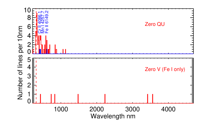
Figure 3.— The numbers of lines known to have zero linear polarization are shown in the top panel as a function of wavelength, taken from SAVV93. In red are shown all the transitions listed, and in blue those transitions that are listed as strong enough to observe, and with no known blend. The lower panel shows transitions with no circular polarization, only of Fe I, taken from the NIST online database of atomic spectra. Blue lines shows those for which oscillator strengths are listed by NIST, the red histogram includes all possible transitions. LS coupling is assumed to be valid. The vertical dashed line shows the atmospheric cutoff at 310 nm.

Sanchez Almeida and Vela Villahoz (1993, henceforth SAVV93) proposed a solution to this problem without full knowledge of ${\bf X}$, prompted in part by a study of polarization properties of the Fe II line at 614.92 nm Lites (1993). When the X matrix satisfies come commonly encountered symmetry properties, measurements of continuum and lines known a priori to generate zero linear polarization, the needed elements of ${\bf X}$ can be algebraically eliminated to a high level of accuracy (see eqs. 4 and 7 of SAVV93). The particular transitions of interest are characterized by peculiar Zeeman patterns where a compensation occurs between $\sigma$ and $\pi$ components, causing the transfer equations for the Stokes parameters $Q$, $U$ to be decoupled from those for $I$ and $V$. When the boundary values for $Q$ and $U$ are also zero (deep in the atmosphere) the emergent linear polarization is then zero. These transitions are:

$${}^{\mathrm{4}}{\rm D}_{\mathrm{1/2}} \rightarrow \ {}^{\mathrm{2S+1}}{\rm L}_{\mathrm{1/2}},$$

$${}^{\mathrm{6}}{\rm G}_{\mathrm{3/2}} \rightarrow \ {}^{\mathrm{2S+1}}{\rm L}_{\mathrm{1/2}},$$

$${}^{\mathrm{22}}{\rm O}_{\mathrm{3/2}} \rightarrow \ {}^{\mathrm{2S+1}}{\rm L}_{\mathrm{1/2}},$$

$$\hskip-26.0pt{\rm where\ }^{\mathrm{2S+1}}{\rm L\neq^{\mathrm{4}}\!D}$$

(See also table 9.4 of Landi Degl’Innocenti and Landolfi, 2004). The latter condition ensures that the LS-coupled Landé g-factors are non-zero, and therefore $V\neq 0$. A list of these lines, assuming LS coupling is valid, is given in Table 1 of Vela Villahoz et al. (1994). The transitions belong only to atomic systems with odd numbers ($n=3,5,7...$) of electrons, thus excluding the rich spectrum of Fe I from the Sun’s photosphere.

Of 86 such lines listed by Vela Villahoz et al. (1994), just 3 are unblended, lying above the Earth’s atmospheric cutoff at 310 nm and which belong to an abundant element ($>10^{\mathrm{-6}}\times$ hydrogen). Figure 3 shows, in the upper panel, those lines compiled by Vela Villahoz et al. (1994) that satisfy the constraints of equation (5.1). The three lines in the visible region which remain sufficiently unblended to be of real practical use, are marked in blue.

5.2. Lines with linear but no circular polarization?

The analysis of SAVV93 suggests that, if lines with $V=0$ but with non-zero $Q$ and $U$ genuinely exist, then their analysis might be extended to try to recover the full Stokes vector S. But citing Makita (1986, in particular figure 9), SAVV93 note that even if the Landé g-factor is zero, magneto-optical effects can produce circular polarization. Such polarization is generally small (Landi Degl’Innocenti and Landolfi, 2004, section 9.22), being of order $\epsilon_{\mathrm{Z}}^{\mathrm{4}}$ for Stokes $V$ in the weak field case.

Landstreet (1969) searched Moore’s 1945 revised multiplet table for LS coupled transitions with zero Zeeman splitting in the presence of magnetic fields. The $g=0$ levels, when connected with either a $J=0$ of $g=0$ level generate no Zeeman-induced polarization at all since the levels are unsplit. The 709.04 nm transition of Fe I (${\rm 5s\,^{\mathrm{5}}F_{\mathrm{1}}\rightarrow 4p\,^{\mathrm{5}}D^{\mathrm{o}}_{\mathrm{0}}}$, both with the ${\rm 3p^{\mathrm{6}}3d^{\mathrm{7}}(^{\mathrm{4}}F)}$ core) is an example, the absence of polarization of this line is seen in Figure 1, showing that such lines can useful as limited checks of calibration procedures.

However, we need transitions for which $V=0$ but for which $Q,U$ are non-zero, in order that we can determine the needed elements of X. Table 9.4 of Landi Degl’Innocenti and Landolfi (2004) lists several such transitions, which are mostly spin-forbidden, and most of which also require $\Delta{\rm L}=2$:

$${}^{\mathrm{6}}{\rm P}_{\mathrm{3/2}} \rightarrow\ ^{\mathrm{4}}{\rm F}_{\mathrm{5/2}}, \ (\Delta{\rm S}=1,\Delta{\rm L}=2)$$

$${}^{\mathrm{5}}{\rm D}_{\mathrm{2}} \rightarrow\ ^{\mathrm{3}}{\rm G}_{\mathrm{3}}, \ (\Delta{\rm S}=1,\Delta{\rm L}=2)$$

$${}^{\mathrm{7}}{\rm D}_{\mathrm{1}} \rightarrow\ ^{\mathrm{5}}{\rm F}_{\mathrm{2}}, \ (\Delta{\rm S}=1,\Delta{\rm L}=1)$$

$${}^{\mathrm{8}}{\rm D}_{\mathrm{5/2}} \rightarrow\ ^{\mathrm{6}}{\rm G}_{\mathrm{7/2}}, \ (\Delta{\rm S}=1,\Delta{\rm L}=2)$$

$${}^{\mathrm{5}}{\rm F}_{\mathrm{2}} \rightarrow\ ^{\mathrm{5}}{\rm H}_{\mathrm{3}}, \ (\Delta{\rm S}=0,\Delta{\rm L}=2)$$ (10)

$${}^{\mathrm{7}}{\rm F}_{\mathrm{2}} \rightarrow\ ^{\mathrm{7}}{\rm H}_{\mathrm{3}}, \ (\Delta{\rm S}=0,\Delta{\rm L}=2)$$

$${}^{\mathrm{7}}{\rm F}_{\mathrm{3}} \rightarrow\ ^{\mathrm{5}}{\rm H}_{\mathrm{4}}, \ (\Delta{\rm S}=1,\Delta{\rm L}=2)$$

$${}^{\mathrm{8}}{\rm F}_{\mathrm{3/2}} \rightarrow\ ^{\mathrm{6}}{\rm G}_{\mathrm{5/2}}, \ (\Delta{\rm S}=1,\Delta{\rm L}=1)$$

The conditions for the existence of lines with “$V=0$” and “$Q,U\neq 0$” are interesting. In order to produce transitions of electric dipole (E1) character at all, the level(s) involved must be mixed by spin-orbit or similar interactions, since under strict LS coupling these are spin- and/or total angular momentum- forbidden. But this also means that the Landé g-factors of the mixed levels must be non-zero. (Alternatively, such transitions might be magnetic dipole, or quadrupolar transitions, but these will be much weaker for neutrals or singly ionized ions). When such E1-type mixing occurs, then with (Cowan, 1981)

$$|\alpha J\rangle=\sum_{\mathrm{\gamma SL}}|\gamma SLJ\rangle\langle\gamma SLJ|\alpha J\rangle$$ (11)

the Zeeman splitting of the mixed level is

$$g_{\mathrm{\alpha J}}=\sum_{\mathrm{\gamma SL}}g_{\mathrm{SLJ}}\ |\langle\gamma SLJ|\alpha J\rangle|^{\mathrm{2}}.$$ (12)

For a spin-forbidden (SF) transition, the same mixing induces the radiative transition via a fully permitted E1 transition. For illustration, if just one level is mixed with one other, say the $|^{\mathrm{5}}{\rm F}_{\mathrm{2}}\rangle$ level is actually $|^{\mathrm{5}}{\rm F}_{\mathrm{2}}\rangle+\epsilon|^{\mathrm{7}}{\rm F}_{\mathrm{2}}\rangle$, $|\epsilon|\ll 1$, then the E1 line strength ${\cal S}(\propto gf)$ is

$${\cal S}(^{\mathrm{7}}{\rm D}_{\mathrm{1}}\rightarrow\ ^{\mathrm{5}}{\rm F}_{\mathrm{2}})\approx\epsilon^{\mathrm{2}}\ {\cal S}(^{\mathrm{7}}{\rm D}_{\mathrm{1}}\rightarrow\ ^{\mathrm{7}}{\rm F}_{\mathrm{2}})$$ (13)

It is clear that there is in principle no transition with finite Q,U and zero V, since the conditions given by (10) and (13) requires a finite mixing coefficient which leads to an, albeit small, modification of a Landé g-factor in equation (12). Since the Landé g-factor of a transition is the combination of g-factors of the two atomic levels involved, each case must be examined to see the effect of the mixing on the Zeeman patterns. But it seems likely, that transitions might be found which will have small enough $g$-factors and small enough magneto-optical effects that they have very small $V$, at the same time having a finite $Q,U$. Equivalent lines for the “zero $Q,U$” case are listed in Table 2 of Vela Villahoz et al. (1994),

We will assume that $V$ is small enough to lie within the noise of solar measurements henceforth. This assumption will be examined in a later publication.

To begin exploring such transitions, we examine the spectrum of Fe I which dominates (by number) the photospheric spectrum of the Sun. The transition ${}^{\mathrm{7}}{\rm D}_{\mathrm{1}}\rightarrow\ ^{\mathrm{5}}{\rm F}_{\mathrm{2}}$ has no entries in the NIST atomic database, but there are semi-empirical $gf$-values from Kurucz . Examples of these Fe I lines in the solar spectrum include 425.6199 nm (log $gf=-2.4$), 728.1564 (log $gf=-4.2$), 830.7606 (log $gf=-5.5$), although the latter two lines are blended with telluric H₂O. There are others predicted at infrared wavelengths including 1.478302, 2.234095, 3.423527, 3.558674, 6.439891 $\mu$m with log $gf$ between -3 and -4. The transitions are marked in Figure 3.

5.3. Feasibility study for vector polarimetry

Here we generalize the approach of SAVV93. Consider that we can observe two lines close together in the spectrum, one known to produce ${\bf S_{\mathrm{1}}=}(I_{\mathrm{1}},0,0,V_{\mathrm{1}})^{\mathrm{T}}$, the other ${\bf S_{\mathrm{2}}=}(I_{\mathrm{2}},Q_{\mathrm{2}},U_{\mathrm{2}},\epsilon)^{\mathrm{T}}$, with $\epsilon\ll 1$. For convenience, we will assume $\epsilon=0$ below, i.e. it lies below the noise levels. Like SAVV93, we will assume we can measure the neighboring continuum with ${\bf S_{\mathrm{0}}=}(I_{\mathrm{0}},0,0,0)^{\mathrm{T}}$. Now make measurements of these lines and continuum wavelengths simultaneously, each one obeying equation (6). Each of the three arrays ${\bf S_{\mathrm{i}}}$ yields an array of (at least) four counts C

$${\bf C_{\mathrm{i}}=(MX)_{\mathrm{i}}S_{\mathrm{i}}}.$$ (14)

In a weakly polarizing telescope ${\bf X}$ obeys certain symmetries (see equation A3.a of SAVV93), leaving just 7 independent matrix elements (one on the diagonal and 6 off-diagonal). X must be of the form

$${\bf X}=g\begin{bmatrix}1&a&b&c\\ a&1&d&e\\ b&-d&1&f\\ c&-e&-f&1\\ \end{bmatrix}$$

usually with $|a|,|b|,|c|,|d|,|e|,|f|\ll 1$ and $g$ can be considered a calibration factor (counts per unit intensity), assumed fixed during the observations. The small values of $|a|\ldots|f|$ are not important, but the symmetries are, we will obtain solutions only when there are at most seven variables $a\ldots g$. X matrices for the DKIST have been studied by Harrington and Sueoka (2016), broken down into primary, secondary and Coudé feed optics and finally instrument optics. They conclude that after the Gregorian (secondary mirror, “M2”) reflection

“Only the IQ and QI terms have substantial amplitude [$\approx 0.27\%$] the lack of cancellation from M2 reversing the sign of the reflection.”

Simulated images across the 5 arcminute FOV show that the matrices are close to the weakly polarizing form. Thus, a modulator placed immediately after M2 would satisfy the requirements for application of the proposed formalism.

Further down the optical chain, before the proposed modulators for the VTF, ViSP, and DL-NIRSP instruments, the X matrices of Harrington and Sueoka (2016) appear to exhibit the symmetries of the above weakly polarizing matrix, but $d,e,f$ ($QUV$ to $QUV$ crosstalk terms) can become large as the telescope rotates while tracking the Sun. We will assume henceforth that our model, relying only on the symmetry properties, can be applied to DKIST.

Thus our goal is to determine all the independent elements ${\bf S_{\mathrm{i}}}$, relative to the continuum intensity, plus the six coefficients $a$-$f$ of the X matrix, given the twelve measurements made with the specific input Stokes ${\bf S_{\mathrm{0}},S_{\mathrm{1}},S_{\mathrm{2}}}$ with the properties detailed above.

Let us assume that the counts have been dark and gain corrected. “Analyzing” (i.e. applying calibrated matrices M after the modulator stage; this could be done infrequently in the fixed frame of the Coudé lab) without knowledge of X produces the set of ”measured” Stokes parameters c’_i using

$${\bf c^{\prime}_{\mathrm{i}}=(M^{\mathrm{T}}M)^{\mathrm{-1}}C_{\mathrm{i}}=X_{\mathrm{i}}S_{\mathrm{i}}}.$$ (15)

For the continuum measurements (${\bf S=S_{\mathrm{0}}}$), dividing all intensities ${\bf c^{\prime}}$ by the measured intensity $=gi_{\mathrm{0}}$ then

$${\bf c_{\mathrm{0}}}={\bf c^{\prime}_{\mathrm{0}}}/gi_{\mathrm{0}}=(1,q_{\mathrm{0}},u_{\mathrm{0}},v_{\mathrm{0}})^{\mathrm{T}}=(1,a,b,c)^{\mathrm{T}}.$$ (16)

$a,b$ and $c$ are thus known from the measured counts in each demodulated state $(q_{\mathrm{0}},u_{\mathrm{0}},v_{\mathrm{0}})$ divided by the continuum intensity. For the case studied by SAVV93 (${\bf S=S_{\mathrm{1}}}$, no linear polarization): ${\bf c_{\mathrm{1}}}=\begin{bmatrix}i_{\mathrm{1}}\\ q_{\mathrm{1}}\\ u_{\mathrm{1}}\\ v_{\mathrm{1}}\\ \end{bmatrix}$ $=\begin{bmatrix}I_{\mathrm{1}}+cV_{\mathrm{1}}\\ aI_{\mathrm{1}}+eV_{\mathrm{1}}\\ bI_{\mathrm{1}}+fV_{\mathrm{1}}\\ cI_{\mathrm{1}}+V_{\mathrm{1}}\\ \end{bmatrix}$ where the $(i_{\mathrm{1}},q_{\mathrm{1}},u_{\mathrm{1}},v_{\mathrm{1}})$ are again all relative to $i_{\mathrm{0}}$, the continuum intensity. These four equations have four unknowns $I_{\mathrm{1}},V_{\mathrm{1}},e,f$ which can be solved for algebraically. This completes the essence of the analysis of SAVV93.

For the new case (S=S₂, negligible circular polarization) we have the measurements ${\bf c_{\mathrm{2}}}=\begin{bmatrix}i_{\mathrm{2}}\\ q_{\mathrm{2}}\\ u_{\mathrm{2}}\\ v_{\mathrm{2}}\\ \end{bmatrix}$ $=\begin{bmatrix}I_{\mathrm{2}}+aQ_{\mathrm{2}}+bU_{\mathrm{2}}\\ aI_{\mathrm{2}}+Q_{\mathrm{2}}+dU_{\mathrm{2}}\\ bI_{\mathrm{2}}-dQ_{\mathrm{2}}+U_{\mathrm{2}}\\ cI_{\mathrm{2}}-eQ_{\mathrm{2}}-fU_{\mathrm{2}}\\ \end{bmatrix}$ which is another set of four equations for the last four remaining unknowns $I_{\mathrm{2}},Q_{\mathrm{2}},U_{\mathrm{2}}$ and $d$. Although, unlike the previous cases, these four equations are non-linear in the unknowns. The equations for $q_{\mathrm{2}}$ and $u_{\mathrm{2}}$ can be used to eliminate $d$, yielding 3 equations for $I_{\mathrm{2}},Q_{\mathrm{2}}$ and $U_{\mathrm{2}}$ for example. But the equations are quadratic and the closed solutions are very lengthy, since the elimination of unknown $d$ gives

$$Q_{\mathrm{2}}^{\mathrm{2}}+U_{\mathrm{2}}^{\mathrm{2}}+I_{\mathrm{2}}(aQ_{\mathrm{2}}+bU_{\mathrm{2}})-u_{\mathrm{2}}U_{\mathrm{2}}-q_{\mathrm{2}}Q_{\mathrm{2}}=0,$$ (17)

and the remaining equations are of the form $Q_{\mathrm{2}}=\alpha+\beta I_{\mathrm{2}}$, $U_{\mathrm{2}}=\gamma+\delta I_{\mathrm{2}}$.

This completes the simple formalism proposed here for using specific atomic transitions to enable accurate and straightforward polarimetry through a polarizing optical system.

There are several potential difficulties with this proposal that will be discussed in a later publication. For now, we address some difficulties in the next section.

Table 2Close pairs of lines where $``Q,U=0"$ and Fe I $``V=0"$

Zero QU		Zero V		$\Delta\lambda$ nm
Ion	$\lambda$ nm	Ion	$\lambda$ nm
Mn I	425.770	Fe I	425.6199	0.15
Fe I	426.53	Fe I	425.6199	0.91
Fe I	730.06	Fe I	728.1564	1.91

All $V=0$ and $Q,U\neq 0$ lines of Fe I discussed in the text are grouped with nearby lines in Tables 1 and 2 of Vela Villahoz et al. (1994). Further work is in progress to find lines of ions with “$V=0$”, other than for Fe I.

6. Outlook

We have reviewed how lines with no linear and/or very small circular polarization might help us measure polarized light reliably through a large polarizing telescope/instrument system. We have adopted the LS coupling scheme with single, unmixed configurations in this overview, with the necessary exception of the spin-forbidden transitions leading to transitions with large $Q,U$ but small or negligible $V$ (section 5.2). It remains to be seen if lines can be found which are strong enough (big $gf$) but with small circular polarization to permit the application of the ideas presented in section 5.3. Further, the analysis presented there must be shown to yield well-posed physical solutions to equation (17). These points will be addressed in a publication that is currently under preparation.

Existing transition data for the “$V=0$” spin-forbidden transitions appear to be, for the important spectrum of Fe I, entirely from semi-empirical work by Kurucz . It would seem important to revisit ab-initio calculations of this ion. It is possible that existing data are of insufficient accuracy to provide important information for application to the kind of solar spectropolarimetry advocated here.

The most obvious needs for new atomic data include the following:

• Infrared lines. The DKIST will at first light (2019) be equipped with powerful spectropolarimeters operating out to 5$\mu$m, yet most reliable atomic parameters for the most useful spectral lines in this range (wavelengths, mixing coefficients, Landé g-factors, oscillator strengths) are either unavailable or semi-empirical in nature, the most reliable being measured at shorter wavelengths.

• Spin-forbidden lines of iron group neutrals and singly-charged ions. Further experiments and ab-initio systematic studies would be especially useful to obtain reliable atomic parameters for the lines matching the conditions given by equation (10). Focus might be placed upon both magnetically-sensitive IR lines, and near-UV lines which might achieve the highest angular resolutions.

Conversely, it is likely that solar physics will provide new constraints on atomic calculations as the polarization characteristics of many lines are measured for the first time in infrared regions. Thus, mixing coefficients (equations 11 and 12) can be assessed through measurements of polarization of atomic transitions at high sensitivity, for comparison with correlation calculations in complex systems.

In Table 2 we list pairs of atomic transitions of abundant ions in which both lines of type $``Q,U=0"$ as well as lines of type $``V=0"$ could be observed over a limited spectral range. We call these “calibration pairs”. We chose a 2 nm width in constructing this table in order to list a potentially useful line pair, noting that this exceeds the spectral range of the current ViSP design for DKIST. Even so, it is clear that a small but non-zero number of pairs are available for study. It should also be noted that problems of both blending and weak magnetic sensitivity are improved by moving to IR wavelengths, for which several “$V=0$” spin-forbidden transitions of Fe I have been computed by Kurucz. Perhaps further calculations and laboratory work up to 5 $\mu$m is warranted.

Lastly, generally speaking the two lines of each calibration pair are formed in different regions of the Sun’s atmosphere, with perhaps some overlap. Therefore, the particular measurements of ${\bf S_{\mathrm{i}}}$ determined above must be augmented with other data to determine the vector magnetic field from a particular region. But the main point here is that the six coefficients $a$-$f$ of X are determined, and can be applied to any line close enough in wavelength to each “calibration” pair.

References

- Babcock (1953) Babcock, H. W.: 1953, Astrophys. J. 118, 387
- Babcock and Babcock (1952) Babcock, H. W. and Babcock, H. D.: 1952, Publ. Astron. Soc. Pac. 64, 282
- Berger et al. (1998) Berger, T. E., Löfdahl, M. G., Shine, R. A., and Title, A. M.: 1998, Astrophys. J. 506, 439
- Cameron et al. (2011) Cameron, R., Vögler, A., and Schüssler, M.: 2011, A&A 533, A86
- Casini and Landi Degl’Innocenti (2008) Casini, R. and Landi Degl’Innocenti, E.: 2008, Plasma Polarization Spectroscopy, Chapt. 12. Astrophysical Plasmas, 247, Springer
- Cowan (1981) Cowan, R. D.: 1981, The Theory of Atomic Structure and Spectra, University of California Press, Berkeley CA
- Denker et al. (2012) Denker, C., Lagg, A., Puschmann, K. G., Schmidt, D., Schmidt, W., Sobotka, M., Soltau, D., Strassmeier, K. G., Volkmer, R., von der Luehe, O., Solanki, S. K., Balthasar, H., Bello Gonzalez, N., Berkefeld, T., Collados Vera, M., Hofmann, A., and Kneer, F.: 2012, IAU Special Session 6, E2.03
- Dufton and Kingston (1981) Dufton, P. L. and Kingston, A. E.: 1981, Adv. At. Molec. Phys. 17, 355
- Gabriel and Jordan (1971) Gabriel, A. H. and Jordan, C.: 1971, Case Studies in Atomic Collision Physics, Chapt. 4, 210–291, North-Holland
- Goode and Cao (2012) Goode, P. R. and Cao, W.: 2012, in T. R. Rimmele, A. Tritschler, F. Wöger, M. Collados Vera, H. Socas-Navarro, R. Schlichenmaier, M. Carlsson, T. Berger, A. Cadavid, P. R. Gilbert, P. R. Goode, and M. Knölker (Eds.), Second ATST-EAST Meeting: Magnetic Fields from the Photosphere to the Corona., Vol. 463 of Astronomical Society of the Pacific Conference Series, 357
- Harrington and Sueoka (2016) Harrington, D. and Sueoka, S. R.: 2016, Vol. 9912, Proc SPIE
- Keil et al. (2009) Keil, S., Rimmele, T., and Wagner, J.: 2009, Earth, Moon and Planets 104, 77
- (13) Kurucz, R. L., in M. McNally (Ed.), Trans. IAU, XXB, Dordrecht: Kluwer, p. 168
- Landi Degl’Innocenti (2013) Landi Degl’Innocenti, E.: 2013, Memorie della Societa Astronomica Italiana 84, 391
- Landi Degl’Innocenti and Landolfi (2004) Landi Degl’Innocenti, E. and Landolfi, M.: 2004, Polarization in Spectral Lines, Vol. 307 of Astrophysics and Space Science Library
- Landstreet (1969) Landstreet, J. D.: 1969, Publ. Astron. Soc. Pac. 81, 896
- Lites (1993) Lites, B. W.: 1993, Solar Phys. 143, 229
- Makita (1986) Makita, M.: 1986, Solar Phys. 106, 269
- Parker (1979) Parker, E. N.: 1979, Cosmical magnetic fields, Clarendon Press, Oxford
- Parker (2009) Parker, E. N.: 2009, Space Sci. Rev. 144, 15
- Rimmele and Marino (2011) Rimmele, T. and Marino, J.: 2011, LRSP 8, 2