Shell model results for $T=1$ and $T=0$ bands in ⁶⁶As

Abstract

Results of a comprehensive shell model (SM) analyses, within the full $f_{5/2}pg_{9/2}$ model space, of the recently available experimental data [P. Ruotsalainen et al., Phy. Rec. C 88, 024320 (2013)] with four $T=0$ bands and one $T=1$ band in the odd-odd $N=Z$ nucleus ⁶⁶As are presented. The calculations are performed using jj44b effective interaction developed recently by B.A. Brown and A.F. Lisetskiy for this model space. For the lowest two $T=0$ bands and the $T=1$ band, the results are in reasonable agreement with experimental data and deformed shell model is used to identify their intrinsic structure. For the $T=1$ band, structural change at $8^{+}$ is predicted. For the third $9^{+}$ band with $T=0$, the shell model $B(E2)$ values and quadrupole moments (in addition to energies) are consistent with the interpretation in terms of aligned isoscalar $np$ pair in $g_{9/2}$ orbit coupled to the ⁶⁴Ge ground band. Similarly, the $9^{+}$ level of band 4 and a close lying $5^{+}$ level are found to be isomeric states in the analysis. Finally, energies of the band 5 members calculated using shell model with both positive and negative parity show that the observed levels are most likely negative parity levels. The SM results with jj44b are also compared with the results obtained using JUN45 interaction.

I Introduction

There has been considerable interest in investigating the structure of the nuclei in the mass region $A=60-100$ and in particular even-even and odd-odd $N=Z$ nuclei. The $N=Z$ nuclei in this mass region lie near the proton drip-line. The even-even $N=Z$ nuclei in this region exhibit rapid changes in nuclear shape and nuclear structure with changing nucleon number. For example, ⁶⁴Ge exhibits $\gamma$-soft structure Sta-07 , ⁶⁸Se exhibits oblate shape in the ground state 68se , ⁷²Kr 72kr1 ; 72kr2 ; 72kr3 exhibits shape coexistence, ⁷⁶Sr and ⁸⁰Zr have large ground state deformations 76Sr ; Lister-87 and so on. Recently, evidence for a spin-aligned neutron-proton isoscalar paired phase has been reported from the level structure of ⁹²Pd cederwall . Similarly, $\beta$ decay of the $T=1$ ($J^{\pi}=0^{+}$) and $T=0$ ($J^{\pi}=9^{+}$) isomers in ⁷⁰Br have been recently reported in Ref. 70Br_PRC95 . Also many even-even $N=Z$ nuclei in this region are of astrophysical interest since they are waiting point nuclei for rp-process nucleosynthesis Fuller . Though even-even $N=Z$ nuclei are important and interesting, in the recent years there has been special focus on odd-odd $N=Z$ nuclei as these nuclei are expected to give new insights into neutron-proton ($np$) correlations that are hitherto unknown.

With the development of radioactive ion beam facilities and large detector arrays, new experimental results for the energy spectra of $N=Z$ odd-odd nuclei starting from ⁶²Ga to ⁸⁶Tc are now available in this region; see ks-book and references cited therein. These studies have opened up challenges in describing and predicting spectroscopic properties of these nuclei. In comparison to lighter $fp$ shell nuclei, production cross section in fusion-evaporation reactions become very small for nuclei north of ⁵⁶Ni. The recent development of the recoil-$\beta$-tagging technique provides a tool to study medium-mass nuclei around the $N=Z$ line. Using this several $T=0$ and $T=1$ levels in the odd-odd $N=Z$ ⁶²Ga nucleus were identified in Ga62 . Recently, we have been successful in using the shell model (SM) and deformed shell model (DSM) with jj44b interaction (due to Brown and Lisetskiy jj44b ) to study comprehensively the $T=0$ and the $T=1$ bands/levels in ⁶²Ga Ga62-smdsm . Turning to the next odd-odd $N=Z$ nucleus ⁶⁶As, recently large number of excited states of ⁶⁶As were populated using ⁴⁰Ca(²⁸Si,$pn$)⁶⁶As fusion-evaporation reaction at beam energies of 75 and 83 MeV by Jyväskylä group 66as . Also in this experiment half-lives and ordering of the two known isomeric states ($5^{+}$ at 1354 keV and $9^{+}$ at 3021 keV) have been determined with improved accuracy. Besides this, the experimental data has resulted in identifying five bands in this nucleus.

Theoretical studies for low-lying and low spin $T=0$ and $T=1$ states of ⁶⁶As were carried out using shell model (SM) 66as , deformed shell model (DSM) sk1 and IBM-4 ibm-4 in the past. The above SM calculation was performed using the JUN45 interaction jun45 and similarly, the DSM calculations used a much older interaction due to Madrid-Strasbourg group No-01 . Similarly, IBM-4 uses a Hamiltonian obtained using a mapping procedure that employs the underlying $SU(4)$ algebra. The aim of the present study is to explain, more comprehensively, the recent experimental data for ⁶⁶As using shell model (SM) and to bring out the structure of all the five bands observed in this nucleus by employing the same jj44b interaction we used before for ⁶²Ga. In addition, DSM ks-book is also used to bring out the structure of the intrinsic states generating bands 1-3 of this nucleus. Some of the results presented in this paper are first reported in rila-2016 ; pcs(R) . As discussed ahead, the shell model results for band 4 (high-spin states) are explained using Cranked Nilsson-Strutinsky (CNS) calculations pcs(R) . Now we will give a preview.

Section II gives the model space, effective interaction and other calculation details. The structure of each of the five observed bands are discussed using SM in Sections III.A to III.E. Results are also compared with those from other calculations where available. Finally, concluding remarks are drawn in Sect. IV.

II Method of calculations

In the SM calculation, ⁵⁶Ni is taken as the inert core with the spherical orbits $1p_{3/2}$, $0f_{5/2}$, $1p_{1/2}$ and $0g_{9/2}$ forming the basis space. The jj44b interaction developed by Brown and Lisetskiy jj44b has been used in both the calculations. This interaction was developed by fitting with 600 binding energies and excitation energies of nuclei with $Z=28-30$ and $N=48-50$ available in this region. Here, 30 linear combinations of $JT$ coupled two-body matrix elements (TBME) are varied giving the rms deviation of about 250 keV from experimental data. The single particle energies (spe) are taken to be $-9.6566$, $-9.2859$, $-8.2695$ and $-5.8944$ MeV for the $p_{3/2}$, $f_{5/2}$, $p_{1/2}$ and $g_{9/2}$ orbits, respectively jj44b . Shell model calculations are performed using the shell model code Antoine antoine . The maximum matrix dimension in $M$-scheme is for $0^{+}$ states ( $>$ $21$ million).

In DSM, using the same set of single particle (sp) orbitals, spe and TBME, as used in the SM calculation, the lowest energy intrinsic states (prolate and oblate) for ⁶⁶As are obtained by solving the Hartree-Fock (HF) single particle equation self-consistently assuming axial symmetry. Excited intrinsic configurations are obtained by making particle-hole excitations over the lowest intrinsic state. Good angular momentum states are projected from different intrinsic states and after isospin projection and orthonormalization, band mixing calculations are performed as described in ks-book . Fig. 1 gives the HF sp spectrum for both prolate and oblate solutions. The total isospin for the lowest configurations shown in Fig. 1 is clearly $T=0$. By making particle-hole excitations for the six nucleons out side the lowest $k$ orbit, we have considered 114 configurations as given in rila-2016 and they generate forty four $T=0$ and fifty $T=1$ deformed configurations.

Figure 1: HF single-particle spectra for ⁶⁶As corresponding to the lowest prolate and oblate configurations. In the figure circles represent protons and crosses represent neutrons. The HF energy (E) in MeV, mass quadrupole moment (Q) in units of the square of the oscillator length parameter and the total azimuthal quantum number K of the lowest intrinsic states are given in the figure.

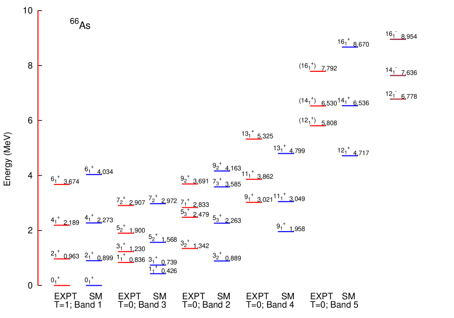
Figure 2: Comparison of shell model results with experimental data for different bands with jj44b interaction. The band numbers in the figure are as per the convention used in the experimental paper 66as . The jj44b interaction predicting isomeric $5^{+}$ state at 985 keV, while experimental value is 1354 keV. We have not shown this state in the present figure.

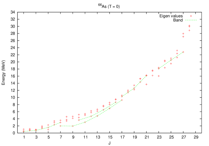
Figure 3: Shell model predictions for different bands in ⁶⁶As.

Figure 4: Comparison of deformed shell model results with experimental data for different bands with jj44b interaction.

III Results and discussions

In Fig. 2, the SM results for $T=0$ and $T=1$ bands are compared with experiment. In SM many levels are calculated (for each $J^{\pi}$) and they are classified into different bands on the basis of dominant $E2$ transitions between them. As shown in Fig.  3, for identifying band structures, we have connected by lines the states with strong transition matrix elements between them and with similar dominant configuration in the wave functions. Occupancies of the orbits for the levels in various bands are shown in Table I. In DSM, calculated levels are classified into bands based on the dominant intrinsic configuration ks-book and the results are shown in Fig.  4 for the lowest 3 bands. The agreements with experiment are reasonable for SM for all the five bands and for the lowest three bands for DSM. We will discuss below the structure of these bands in detail and also compare the results with those obtained using JUN45 interaction reported in 66as .

Table 1: Shell model occupancies for $T=0$ and $T=1$ bands with jj44b/JUN45 interactions. We have shown occupancies of band 1, band 2, band 3 and band 4 with JUN45 for comparison.

	nucleon occupation numbers
	$n_{lj}^{\pi}$ = $n_{lj}^{\nu}$ ($p_{3/2}$,$f_{5/2}$, $p_{1/2}$, $g_{9/2}$)
T=1	Band 1
$0^{+}$	1.97/2.49  1.81/1.49  0.56/0.66  0.66/0.36
$2^{+}$	1.89/2.35  1.91/1.60  0.56/0.69  0.64/0.35
$4^{+}$	1.83/2.42  2.00/1.64  0.53/0.62  0.64/0.32
$6^{+}$	1.79/2.30  2.09/1.82  0.48/0.57  0.64/0.30
$8^{+}$	1.45/2.60  1.92/1.76  0.47/0.42  1.16/0.21
T=0	Band 2
$3^{+}$	2.12/2.49  1.87/1.64  0.48/0.59  0.53/0.27
$5^{+}$	2.15/2.49  1.81/1.69  0.52/0.59  0.52/0.22
$7^{+}$	1.34/1.59  2.00/1.86  0.37/0.47  1.28/1.07
$9^{+}$	1.50/2.08  1.77/2.19  0.49/0.54  1.24/0.19
T=0	Band 3
$1^{+}$	1.96/2.47  2.03/1.60  0.53/0.67  0.48/0.25
$3^{+}$	1.91/2.46  2.11/1.68  0.51/0.61  0.48/0.25
$5^{+}$	2.52/2.32  1.26/1.85  0.83/0.57  0.39/0.25
$7^{+}$	1.82/2.19  2.21/2.04  0.48/0.53  0.49/0.24
T=0	Band 4
$5^{+}$	2.52/2.74  1.26/1.23  0.83/0.85  0.39/0.18
$9^{+}$	1.48/1.61  1.95/1.86  0.48/0.46  1.09/1.08
$11^{+}$	1.52/1.68  1.88/1.76  0.51/0.49  1.08/1.07
$13^{+}$	1.64/1.76  1.66/1.63  0.63/0.55  1.07/1.06
T=0	Band 5 ($+$ve)
$12^{+}$	1.54  1.89  0.47  1.09
$14^{+}$	1.66  1.74  0.53  1.08
$16^{+}$	1.95  1.36  0.63  1.06
T=0	Band 5 ($-$ve)
$12^{-}$	1.16  1.83  0.43  1.57
$14^{-}$	1.20  1.74  0.45  1.59
$16^{-}$	1.33  1.59  0.51  1.57

Table 2: Comparison of $B(E2)$’s values for different bands with jj44b and JUN45 interactions. Results are in $e^{2}fm^{4}$ with $e_{p}=1.5$e and $e_{n}=0.5$e.

Transitions	jj44b	JUN45
	Band 3
$7^{+}$ $\rightarrow$ $5^{+}$	416.12	374.91
$5^{+}$ $\rightarrow$ $3^{+}$	375.98	333.81
$3^{+}$ $\rightarrow$ $1^{+}$	296.63	204.00
	Band 2
$9^{+}$ $\rightarrow$ $7^{+}$	277.62	0.27
$7^{+}$ $\rightarrow$ $5^{+}$	0.01	0.000
$5^{+}$ $\rightarrow$ $3^{+}$	38.33	55.56
	Band 4
$13^{+}$ $\rightarrow$ $11^{+}$	282.85	266.66
$11^{+}$ $\rightarrow$ $9^{+}$	326.96	306.06

Table 3: $B(M1)$ values in $\mu_{N}^{2}$. Here $g_{s}=g_{free}$ used in the SM calculations.

$I_{f}^{+}\rightarrow I_{i}^{+}$	jj44b
T=1 $\rightarrow$ T=0
$0_{1}^{+}\rightarrow 1_{1}^{+}$	0.16
$2_{1}^{+}\rightarrow 1_{1}^{+}$	0.073
$2_{1}^{+}\rightarrow 3_{2}^{+}$	0.051
$2_{1}^{+}\rightarrow 3_{1}^{+}$	0.023
$4_{1}^{+}\rightarrow 5_{2}^{+}$	0.0048
$4_{1}^{+}\rightarrow 5_{1}^{+}$	0.0052
$6_{1}^{+}\rightarrow 7_{2}^{+}$	0.025
$6_{1}^{+}\rightarrow 7_{1}^{+}$	0.0004

III.1 Band # 1 $(T=1)$

The $T=1$ band (band #1 in Fig.  2) with $0^{+}$, $2^{+}$, $4^{+}$ and $6^{+}$ is well described by shell model and it is the isobaric analogue of the lowest $T=1$ band in ⁶⁶Ge; see nndc ; all the levels are quantitatively reproduced. The DSM calculated $T=1$ band (Fig.  4) also agrees reasonably well with experiment. Except for the $2^{+}\rightarrow 0^{+}$ separation (it is lower compared to experiment by $\sim 300$ keV), the relative spacing of all other levels are reasonably reproduced. This implies that DSM predicts this band to be more collective and hence more compressed compared to data and SM results. The $T=1$ levels up to $J=6^{+}$ mainly originate from the lowest $T=1$ intrinsic state generated by the antisymmetric combination of the configurations $(1/2^{-})_{1}^{2p,2n}\,(1/2^{-})_{2}^{2p,2n}(3/2^{-}\uparrow)_{1}^{p}(3/2^{-}\downarrow)_{1}^{n}$ and $(1/2^{-})_{1}^{2p,2n}\,(1/2^{-})_{2}^{2p,2n}(3/2^{-}\uparrow)_{1}^{n}(3/2^{-}\downarrow)_{1}^{p}$. Hence, there is no change in the collectivity up to $J=6^{+}$. The shell model (SM) as well as the DSM predicts the $B(E2)$ values for the transition $8^{+}\rightarrow 6^{+}$ to be very small (their energies are 5.124 MeV in SM and 3.973 in DSM). For example, the $B(E2)$ ratios $B(E2,I\rightarrow I-2)$ $/B(E2,I-2\rightarrow I-4)$ with I=4, 6, 8 are 1.22, 0.97 and 0.001 in DSM. The corresponding ratios for shell model are 1.29, 1.09 and 0.001. The occupancy of the $1g_{9/2}$ orbit as seen in Table  LABEL:tocc does not change much up to spin $T=1,J=6^{+}$ and is about 0.64 for both protons and neutrons. However, as we go to $T=1,8_{1}^{+}$ level, there is a dramatic change in the $g_{9/2}$ occupancy which is 1.16 in SM. Thus, shell model predicts the structure of the $T=1,8_{1}^{+}$ level to be quite different from that of the other $T=1$ levels lying below. As a result, the $B(E2)$ transition probability from $T=1,8^{+}$ to $T=1,6^{+}$ is small. This is in agreement with the conclusion drawn from the DSM calculation which predicts that the structure of the $T=1,8_{1}^{+}$ level to be quite different from that of the $T=1,6^{+}_{1}$ level. This level originates from the $T=1$ projected intrinsic state in which three protons and three neutrons are distributed in six single particle orbitals. This configuration has a proton and a neutron in $g_{9/2}$ orbit just the occupancy given by SM. With the structure of the $T=1,8^{+}_{1}$ level being quite different from the $T=1,6^{+}_{1}$, its $E2$ transition probability to $T=1,6^{+}_{1}$ level is also small in DSM just as in SM. Let us add that previous SM studies 66as of ⁶⁶As were due to Honma et al using JUN45 jun45 and Hasegawa et al using an extended pairing plus quadrupole interaction Has-2005 . The SM with JUN45 gives 66as the $2^{+}$, $4^{+}$, $6^{+}$ and $8^{+}$ excitation energies to be $0.967$, $2.222$, $3.891$ and $5.604$ MeV respectively. It is seen that the energies of the $T=1$ band members ($2^{+}$, $4^{+}$, $6^{+}$) are slightly better with JUN45 compared to those with jj44b. However, the structure of the $8^{+}$ predicted by JUN45 is quite different with very low $g_{9/2}$ orbit occupancy.

III.2 Band $\#$ 2 ($T=0$)

Coming to the $T=0$ bands, band #2 (as classified in 66as ) is the first $T=0$ band and it is a $3^{+}$ band. It is seen from Fig.  2 that the SM calculated spectrum for band #2 agrees reasonably well with experiment. Though data are not available, $B(E2)$ values within band #2 are calculated and SM gives for $5^{+}_{3}\rightarrow 3^{+}_{2}$, $7^{+}_{3}\rightarrow 5^{+}_{3}$ and $9^{+}_{2}\rightarrow 7^{+}_{3}$ the values to be $38$, $0.010$ and $278$ $e^{2}fm^{4}$. The effective charges used in this work are $e_{p}=1.5e$ and $e_{n}=0.5e$. The results of $B(E2)$ values for different bands with JUN45 and jj44b are shown in the Table II. The small $E2$ transition between $7^{+}_{3}\rightarrow 5^{+}_{3}$ is due to the structural change between these states. The $3^{+}_{2}$ and $5^{+}_{3}$ wave functions is dominated by $0p-0h$ excitation more than 50 %. On the other hand, the $7^{+}_{3}$ and $9^{+}_{2}$ states show (proton-neutron) pair excitation to the $g_{9/2}$ orbit. The occupation of the $1p_{3/2}$ suddenly changes from $\sim$ 2.2 ($3_{2}^{+}$, $5_{3}^{+}$) to $\sim$ 1.3 ($7_{3}^{+}$, $9_{2}^{+}$). This apparent structure change causes the small transition between $7^{+}_{3}\rightarrow 5^{+}_{3}$. Let us add that JUN45 interaction predicts $3^{+}-5^{+}-7^{+}-9^{+}$ states at 995, 2154, 2652 and 4677 keV, respectively. While corresponding jj44b interaction results are 889, 2263, 3585, and 4163 keV, respectively. Also, as seen from the occupancies in Table I and $B(E2)$ for $9/2^{+}$ to $7/2^{+}$ given in Table II, the structure of the $9^{+}$ level in this band predicted by JUN45 is quite different from the structure predicted by jj44b interaction. Finally, Fig. 4 shows the band #2 levels from DSM. It is seen that these levels have admixtures from many intrinsic states (except for the $3^{+}$ level) and therefore DSM do not give this to be a proper collective band. Thus, measuring B(E2)’s in future for band #2 members is important. We have also shown the $M1$ transitions between $T=1$ to $T=0$ states in Table III. These values are very small, although the $B(M1\,6^{+}_{1}\rightarrow 7^{+}_{2})$ estimated to be $\sim$ 1 $\mu_{N}^{2}$ in Ref. 66as . The JUN45 interaction result is also small 66as .

III.3 Band $\#$ 3 ($T=0$)

Band #3 with $T=0$ consists of $1^{+}$, $3^{+}$, $5^{+}$ and $7^{+}$ levels. All these levels except $7^{+}$ level are found to have similar structure both in SM and DSM. They mainly originate, as seen from DSM, from the symmetric combination of the configurations $(1/2^{-})_{1}^{2p,2n}\,(1/2^{-})_{2}^{2p,2n}(3/2^{-}\uparrow)_{1}^{p}(3/2^{-}\downarrow)_{1}^{n}$ and $(1/2^{-})_{1}^{2p,2n}\,(1/2^{-})_{2}^{2p,2n}(3/2^{-}\uparrow)_{1}^{n}(3/2^{-}\downarrow)_{1}^{p}$ with admixtures from the lowest intrinsic state shown in Fig. 1 and several other intrinsic states. Also, for this band, the JUN45 predict $1^{+}-3^{+}-5^{+}-7^{+}$ states at 611, 871, 1520, and 2750 keV, respectively while jj44b predicts at 426, 739, 1568 and 2972 keV, respectively. Experimentally, no measurements have been made regarding the $B(E2)$ values among the levels of this band. In SM, the calculated $B(E2)$’s for $3^{+}_{1}\rightarrow 1^{+}_{1}$, $5^{+}_{2}\rightarrow 3^{+}_{1}$ and $7^{+}_{2}\rightarrow 5^{+}_{2}$ are $297$, $376$ and $416$ $e^{2}fm^{4}$. In addition, the $B(M1)$ value for the transition $1^{+}_{1}$ to ground $0^{+}$ is $0.0832~{}\mu_{N}^{2}$ and measurement of this $B(M1)$ will give a good test of the structure of band #3. The $B(E2)$ for the decay of $3^{+}$ of band #2 to $1^{+}$ of band #3 will also give a good test of the structure of this band and the shell model value for this transition is $0.70$ $e^{2}fm^{4}$.

An important question that is being probed in the recent years is the energy separation between the lowest $T=1$ and $T=0$ levels, i.e. between the ground $0^{+}$ and the excited $1^{+}_{1}$ level shown in Fig.  2. To this end, we have calculated the pairing energy following the procedure discussed in ref. povesplb , i.e. by taking the energy difference of states calculated with the full Hamiltonian jj44b and the Hamiltonian $H_{eff}$ obtained by subtracting from jj44b Hamiltonian the isovector P01 or isoscalar P10 interaction (see Ga62-smdsm ; povesplb for the two-body matrix elements of $P_{01}$ and $P_{10}$ in $j-j$ coupling). We have used $G$ = 0.276 for P01 and $G$ = 0.506 for P10 following Refs. povesplb ; zuker . In the Figs. 5 (a) and (b) we have shown the contribution of the pairing energies for $T=0$ odd spin states and $T=1$ even spin states respectively. For the even $T=1$ levels with $J\leq 6^{+}$, isoscalar pairing plays a larger role, while for $T=0$ levels with $J\leq 9^{+}$, the isovector plays a much greater role. The $T=1$, $J=0$ ground state has an equal contribution of pairing energies from $T=0$ and $T=1$ channels. The total pairing energy for $T=0$, $J=1$ is 2.14 MeV, whereas for $T=1$, $J=0$, the total pairing energy is 2.64 MeV. Thus, our calculation shows, just as seen in data, that the $T=1$ band should be lower compared to the $T=0$ band because of the gain of 0.5 MeV in pairing energy. It may be noted that our SM calculation with jj44b interaction predicts the $T=1$ and $T=0$ band head separation to be 426 keV compared to the experimental value 836 keV as shown in Fig.  2 and 611 keV from JUN45 interaction 66as .

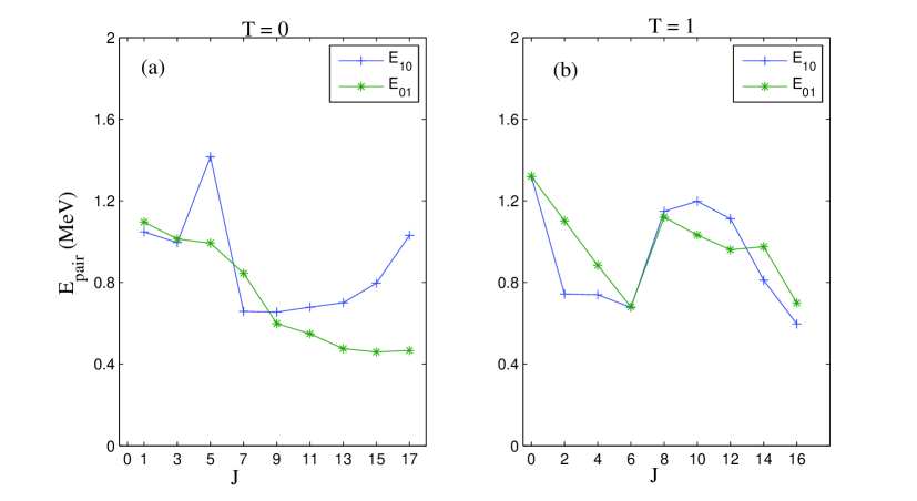
Figure 5: Pairing energies from shell model for (a) $T=0$ odd spin states and (b) $T=1$ even spin states. Here $E_{01}$ and $E_{10}$ are isovector and isoscalar pairing energies respectively.

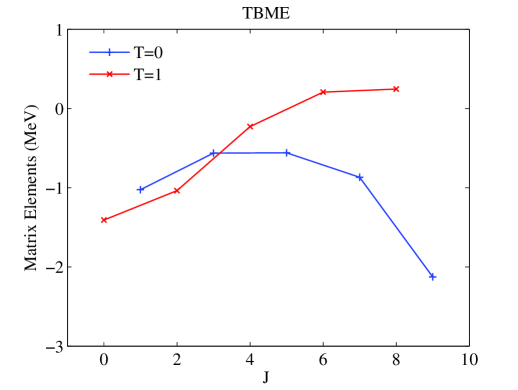
Figure 6: Variation of two-body matrix elements $<(g_{9/2})^{2}J|V|(g_{9/2})^{2}J>$ vs $J$.

III.4 Band $\#$4 ($T=0$)

The band #4 (also with $T=0$), as classified in 66as consists of a level with spin $5^{+}$ at experimental excitation energy 1.354 MeV and in addition $9^{+}$, $11^{+}$ and $13^{+}$ levels; the last three levels are shown in Fig.  2. As we will discuss ahead, the last three levels form a proper band.

III.4.1 $5^{+}$ and $9^{+}$ isomeric states

Firstly, the $5^{+}$ level in SM is predicted at excitation energy 0.985 MeV and DSM predicts the same at 0.893 MeV. However, JUN45 predicts this at 0.407 MeV. From DSM it is seen that this level is essentially generated by the oblate configuration $(3/2^{-})_{1}^{2p,2n}(1/2^{-})_{1}^{2p,2n}(5/2^{-}\uparrow)_{1}^{p,n}$ and the $B(E2)$’s from this level to the $3^{+}$ levels of bands 2 and band 3 are relatively small. Thus, this level is an isomeric state obtained from the totally aligned ${}^{1}f_{5/2}$ $np$ configuration consistent with the claim in 66as . Also, the structure of this $5^{+}$ level is seen to be similar to the $7^{+}$ level of band #3. This is possibly the reason why in the experiment reported in 66as , a large transition strength between these two levels is seen. The present SM calculation with jj44b interaction gives $B(E2,5^{+}_{1}\rightarrow 3^{+}_{1})$ value to be 45 $e^{2}fm^{4}$, DSM gives 1.3 $e^{2}fm^{4}$ and the experimental value 66as is 13 $e^{2}fm^{4}$ (with the effective charges $e_{p}=1.5e$ and $0.5e$). Also as given in 66as , the SM value with JUN45 interaction is 16.02 $e^{2}fm^{4}$ (the effective charges used in Ref. 66as are $e_{p}=1.5e$ and $1.1e$).

Turning to the $9^{+}$ level of band #4, in DSM this level (at excitation energy 5.123 MeV and it is much higher than the experimental value) originates from the oblate intrinsic state with configuration $(3/2^{-})_{1}^{2p,2n}(1/2^{-})_{1}^{2p,2n}(9/2^{+}\uparrow)_{1}^{p,n}$. It has also strong mixing from several prolate intrinsic states. The calculated $B(E2)$ values from this level to the lower $7^{+}$ levels of bands #2 and #3 are relatively small. Thus, this level is also predicted to be a isomeric state with totally aligned $np$ pair in ${}^{1}g_{9/2}$ orbit as the dominant structure and this is consistent with the SM results using JUN45 as reported in 66as . Experimental value for the $B(E2,9^{+}_{1}\rightarrow 7^{+}_{2})$ is 2.6 $e^{2}$$fm^{4}$. The SM values with jj44b interaction is 1.23 $e^{2}$$fm^{4}$ and DSM gives 2.5 $e^{2}$ $fm^{4}$. Finally, SM with JUN45 interaction gives the value 0.22 $e^{2}fm^{4}$ 66as ; note that $7^{+}_{2}$ level belongs to band #3.

III.4.2 $pn$ aligned band with isoscalar $pn$ pair in $g_{9/2}$ orbit

With the $9^{+}$ generated by totally aligned $np$ pair in ${}^{1}g_{9/2}$ orbit, it is plausible that the band 4 with $J=9$, $11$ and $13$ can be interpreted as a band formed out of coupling the ⁶⁴Ge core with a $T=0$ $pn$ pair with the pair in $g_{9/2}$ orbit. Keeping this possibility, the $J^{\pi}=15^{+}$ and $17^{+}$ levels are also calculated in SM with jj44b and they are at energies $6.942$ MeV and $9.285$ MeV respectively. Note that, as angular momentum is increased, more and more particles must be put in the $g_{9/2}$ orbital and this will favor a band at low energy. In Fig. 6, shown are the two-body matrix elements corresponding to $<g_{9/2}g_{9/2}|V|g_{9/2}g_{9/2}>$. From the results in the figure it is clear that the interaction matrix element corresponding to the $(g_{9/2})^{2}$ maximally aligned two-particle state $J^{\pi}$ = $9^{+}$ (and $T=0$) is most attractive (as reported in ref. cederwall -however, the interpretation made in cederwall has been heavily criticized recently in Refs. cr1 ; rob ; fu ; cr3 ) although the $g_{9/2}$ shell is quite high up in energy. With $J=9$ aligned pair acting as a spectator in forming the $T=0$ band in ⁶⁶As with $J$ =9, 11, 13, 15 and 17, the increase of angular momentum simply comes from the core of the remaining particles. Then, we can describe this band by simply considering the ground-state rotational band of the ⁶⁴Ge nucleus (the core) with $J$=0, 2, 4, 6 and 8, and just adding to this band an aligned $pn$-pair providing a constant energy and a constant angular momentum ($=9$); this will be a isoscalar pair.

For further understanding of this band and for suggesting experimental signatures for the structure of this band, $B(E2;J\rightarrow J-2)$ values and spectroscopic quadrupole moments of the levels in band #4 of ⁶⁶As and the levels of the ground band of ⁶⁴Ge are calculated in SM and the results are shown in Fig. 7. Strikingly, as reported in pcs(R) by one of the authors (PCS) with the Lund group, Cranked Nilsson-Strutinsky (CNS) calculations are quite close to the SM results. In CNS, they are generated by the rotation axis flips from the intermediate axis to the smallest axis due to the polarization by the aligned isoscalar $np$ pair in $g_{9/2}$ orbital coupled to the ⁶⁴Ge triaxial core. Thus, ⁶⁶As with band #4 shows spin aligned $np$ isoscalar pair phase as seen before in ⁹²Pd cederwall . As stated in pcs(R) , it is important to test the predicted very small spectroscopic quadrupole moments in ⁶⁴Ge and high moments in ⁶⁶As. Let us add that JUN45 predicts $9^{+}-11^{+}-13^{+}$ states at 2506, 3248, and 4589 keV but there is no discussion of the structure of these levels in 66as where JUN45 results are reported.

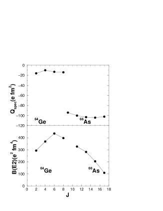
Figure 7: Shell model results for $B(E2;J\rightarrow J-2)$ and spectroscopic quadrupole moments for the levels in band #4 of ⁶⁶As and the ground band of ⁶⁴Ge.

III.5 Band #5 ($T=0$)

Ruotsalainen et al 66as have identified a band of states with $J$=$12^{(+)}$, $14^{(+)}$ and $16^{(+)}$ at energies 5.808, 6.530 and 7.792 MeV. However, they could not assign the parity of these levels uniquely. SM calculations were performed for these levels assuming them to be of positive or negative parity. These levels are shown in Fig.  2 as band #5. Just from the energy systematics, it is more likely that these levels are of negative parity. This is consistent with the prediction from CNS calculations (Ragnarsson, private communication). Experimentally, the collectivity of the levels in band #5 is not known. However, SM predictions for the $B(E2)^{\prime}s$ for $14^{\pm}\rightarrow 12^{\pm}$ and $16^{\pm}\rightarrow 14^{\pm}$ are $298$ ($261$) and $166$ ($332$) $e^{2}fm^{4}$, respectively; numbers in the brackets are assuming negative parity.

IV Conclusions

We have compared the recently available experimental data for $T=0$ and $T=1$ bands for ⁶⁶As with the results obtained from shell model using jj44b interaction.

Following broad conclusions can be drawn:

$\bullet$ The present SM calculations with jj44b interaction describe the observed $T=1$ band (band #1), isobaric analogue of ⁶⁶Ge ground band, reasonably well and predicted a structural change at $8^{+}$. Using DSM it is seen that at $J=8^{+}$ there is band crossing originating due to the occupancy of a proton and a neutron in $g_{9/2}$ orbit.

$\bullet$ We have calculated the pairing energy for $T=0$ and $T=1$ bands (bands #3 and #1). For the $T=0$ band, the contributions from the isoscalar pairing is larger for $J\geq 9^{+}$. Also, the $T=1$ band is predicted (as seen in data) to be lower compared to the $T=0$ band because of a gain of 0.5 MeV in pairing energy.

$\bullet$ The lowest $5^{+}$ level and the $9^{+}$ levels are correctly reproduced by both SM and DSM, with jj44b interaction, to be isomeric states, as found in the shell model and experimental studies reported in 66as ; Has-2005 with quite small $B(E2)$ values involving these levels.

$\bullet$ The results of shell model for band #4 in Fig.  2 are described using ⁶⁴Ge core coupled to a maximally aligned $pn$ $g_{9/2}$ isoscalar pair (with $T=0$ and $J=9$) giving specific predictions for the $B(E2)$ values and quadrupole moments for the members of this band. The shell model results justify a CNS description of this band.

$\bullet$ For band #5, as the parity of the experimental levels is not known, shell model predictions for the excitation energies assuming $+ve$ and $-ve$ parity are given in Section III.

$\bullet$ For a better and complete understanding of the structure of bands #2 and 3 (also #4), $B(E2)$ values involving the levels of these bands are needed in future.

$\bullet$ Comparison of the present SM results obtained using jj44b with those from JUN45 and experimental data showed clearly that jj44b is not able to give as good description of the spectroscopy as we have before for ⁶²Ga Ga62-smdsm . Similarly, as stated in 66as , JUN45 also has problems. Thus, clearly there is need to produce better effective interactions for describing the structure of $N=Z$ nuclei starting from ⁶⁶As.

- (1) K. Starosta et al., Phys. Rev. Lett. 99, 042503 (2007).
- (2) S.M. Fischer et al., Phys. Rev. Lett. 84, 4064 (2000).
- (3) G. de Angelis et al., Phys. Lett. B 415, 217 (1997).
- (4) H. Iwasaki et al., Phys. Rev. Lett. 112, 142502 (2014).
- (5) J. A. Briz et al., Phys. Rev. C 92, 054326 (2015).
- (6) A. Lemasson et al., Phys. Rev. C 85 041303(R) (2012).
- (7) C.J. Lister et al., Phys. Rev. Lett. 59, 1270 (1987).
- (8) B. Cederwall et al., Nature 469, 68 (2011).
- (9) A. I. Morales et al., Phys. Rev. C 95, 064327 (2017).
- (10) J. Pruet and G. M. Fuller, Astrophys. J. Suppl. Ser. 149, 189 (2003).
- (11) V.K.B. Kota and R. Sahu, Structure of Medium Mass Nuclei: Deformed Shell Model and Spin-Isospin Interacting Boson Model (CRC Press, Taylor and Francis group, Florida, 2016).
- (12) H.M. David et al., Phys. Lett. B 726,665 (2013).
- (13) B.A. Brown and A.F. Lisetskiy (unpublished); see also endnote (28) in B. Cheal et al., Phys. Rev. Lett. 104, 252502 (2010).
- (14) P.C. Srivastava, R. Sahu and V.K.B. Kota, Eur. Phys. J. A 51, 3 (2015).
- (15) P. Ruotsalainen et al., Phys. Rev. C 88, 024320 (2013).
- (16) R. Sahu and V.K.B. Kota, Phys. Rev. C 66, 024301 (2002).
- (17) O. Juillet, P. Van Isacker and D.D. Warner, Phys. Rev. C 63, 054312 (2001).
- (18) M. Honma, T. Otsuka, T. Mizusaki and M. Hjorth-Jensen, Phys. Rev. C 80, 064323 (2009).
- (19) E. Caurier, F. Nowacki, A. Poves and J. Retamosa, Phys. Rev. Lett. 77, 1954 (1996).
- (20) R. Sahu and V.K.B. Kota, Nuclear Theory 35, 22 (2016).
- (21) P.C. Srivastava, S. Aberg and I. Ragnarsson, Phys. Rev. C 95, 011303(R) (2017).
- (22) E. Caurier, G. Martínez-Pinedo , F. Nowacki, A. Poves, and A. P. Zuker, Rev. Mod. Phys. 77 (2005) 427.
- (23) http://www.nndc.bnl.gov/ensdf
- (24) M. Hasegawa, Y. Sun, K. Kaneko and T. Mizusaki, Phys. Lett. B 617 (2005) 150-156.
- (25) A. Poves and G. Martinez-Pinedo, Phys. Lett. B 430, 203 (1998).
- (26) M. Dufour and A.P. Zuker, Phys. Rev. C 54, 1641 (1996).
- (27) M. Sambataro and N. Sandulescu, Phys. Rev. C 91, 064318 (2015).
- (28) S. J. Q. Robinson, T. Hoang, L. Zamick, A. Escuderos, and Y. Y. Sharon, Phys. Rev. C 89, 014316 (2014).
- (29) G. J. Fu, J. J. Shen, Y. M. Zhao, and A. Arima, Phys. Rev. C 87, 044312 (2013).
- (30) A. P. Zuker, A. Poves, F. Nowacki, and S. M. Lenzi, Phys. Rev. C 92, 024320 (2015).