Entanglement spectrum degeneracy and Cardy formula in $1+1$ dimensional conformal field theories

Abstract

We investigate the effect of a global degeneracy in the distribution of entanglement spectrum in conformal field theories in one spatial dimension. We relate the recently found universal expression for the entanglement hamiltonian to the distribution of the entanglement spectrum. The main tool to establish this connection is the Cardy formula. It turns out that the Affleck-Ludwig non-integer degeneracy, appearing because of the boundary conditions induced at the entangling surface, can be directly read from the entanglement spectrum distribution. We also clarify the effect of the non-integer degeneracy on the spectrum of the partial transpose, which is the central object for quantifying the entanglement in mixed states. We show that the exact knowledge of the entanglement spectrum in some integrable spin-chains provides strong analytical evidences corroborating our results.

1 Introduction

In the course of the noughties, entanglement has become a standard and powerful tool for the study of many-body quantum systems, both in and out of thermodynamic equilibrium (see, e.g., Refs. [1, 2, 3, 4] as reviews); for example, entanglement is nowadays routinely used for the identification of critical and topological phases of matter. The central quantity to quantify the bipartite entanglement in a many-body system is the reduced density matrix $\rho_{A}$ of a subsystem $A$, which is defined as $\rho_{A}={\rm Tr}_{B}\rho$, where $B$ is the complement of $A$, and $\rho$ is the density matrix of the entire system. When the system is in a pure state $|\Psi\rangle$ and $\rho=|\Psi\rangle\langle\Psi|$, the entanglement can be measured by the von Neumann or Rényi entropies of $\rho_{A}$. However, it has been pointed out long ago by Li and Haldane [5] that the reduced density matrix (RDM) encodes much more information than the entanglement entropy. Part of this information may be extracted by looking at the entire spectrum of $\rho_{A}$, which has been dubbed entanglement spectrum. This observation triggered a systematic study of the entanglement spectrum, which proved to be an extremely powerful theoretical tool to analyse topological phases [5, 6, 7, 8, 9, 10], symmetry-broken phases [11, 12, 13, 14, 15], disordered systems [16, 17, 18, 19], and gapless one-dimensional phases [20, 21, 22]. Furthermore, a protocol for measuring the entanglement spectrum in cold-atom experiments has been proposed [23], which generalises the recent measurements of entanglement entropy [24, 25].

In Ref. [20], it has been pointed out that the distribution of the eigenvalues $\lambda_{i}$ of the reduced density matrix $\rho_{A}$ (also known as entanglement spectrum distribution)

$$P(\lambda)\equiv\sum_{i}\delta(\lambda-\lambda_{i}),$$ (1)

can be reconstructed from the analytic knowledge of the moments ${\rm Tr}\rho_{A}^{n}$ of $\rho_{A}$. In this respect, conformal invariant field theories represent a very useful playground. Indeed, for a conformal invariant system in one spatial dimension, for a finite interval $A$ of length $\ell$ embedded in an infinite system, the moments are given as [26, 27]

$${\rm Tr}\rho_{A}^{n}=c_{n}\Big{(}\frac{\ell}{\epsilon}\Big{)}^{c/6(n-1/n)},$$ (2)

where $c$ is the central charge of the conformal field theory (CFT), $\epsilon$ an ultraviolet cutoff, and $c_{n}$ a non-universal and in general unknown $n$-dependent amplitude. Assuming $c_{n}$ to be constant, in Ref. [20] a super-universal form of the entanglement spectrum distribution has been explicitly worked out: it turned out to depend only on the central charge via the largest eigenvalue of $\rho_{A}$. Thus, when expressed in term of the latter, the entanglement spectrum distribution does not depend on any parameter of the theory. This super-universal distribution leads to an extremely simple scaling law for the integrated distribution function $n(\lambda)$, i.e. the number of eigenvalues larger than $\lambda$, which is

$$n(\lambda)=I_{0}(\xi_{\lambda})\,,\qquad\xi_{\lambda}\equiv 2\sqrt{(-\ln\lambda_{\rm max})\ln(\lambda_{\rm max}/\lambda)}\,,$$ (3)

where $I_{0}(x)$ is the modified Bessel function and $\lambda_{\rm max}$ the largest eigenvalues of $\rho_{A}$. Obviously, the only condition for the validity of (3) is the particular $n$-dependence in (2). Consequently, the same law (3) is valid in many other situations in CFT (finite systems, systems with boundaries, finite temperature, etc), as well as in proximity of quantum critical points, where the same scaling (2) holds with the replacement of $\ell$ with the correlation length [26]. Several numerical studies [20, 28, 29, 30, 31, 4] tested that the super-universal distribution (3) describes surprisingly well the spectrum of lattice models whose low-energy spectrum has an underlying CFT, despite the assumption of $c_{n}$ being constant. The exact knowledge of the distribution (3) played also a central role in the understanding of the performance of matrix product states algorithms [32].

In very recent times, a lot of activity has been devoted also to the study of the operatorial form of the reduced density matrix [33, 34, 35, 36, 37, 38, 39, 40, 41, 42, 43, 44, 45, 46]. To this goal, the reduced density matrix is written as

$$\rho_{A}=\,e^{-2\pi K_{A}},$$ (4)

where $K_{A}$ is the entanglement (or modular) hamiltonian. The first study of the modular Hamiltonian dates back to the seminal work by Bisognano and Wichmann [47], which proved that for an arbitrary relativistic quantum field theory in Minkowski space of generic dimensionality and for a bipartition in two equal semi-infinite parts separated by an infinite hyperplane, the entanglement Hamiltonian may be expressed as an integral of the local energy density with a space-dependent weight factor. This theorem has been exploited, especially in CFTs in arbitrary dimension, to relate entanglement Hamiltonians in different bipartitions [36, 38, 42]. In turn, these works relate the entanglement to the Hamiltonian spectrum, a result which we will exploit here.

This paper has many different goals which can be summarised as follows. On the one hand, we want to directly derive the entanglement spectrum distribution in [20] from the entanglement Hamiltonian in [42], also to understand the validity of the assumptions made in both [42] and [20]; in particular, the assumption of $c_{n}$ being constant (see (2)). We anticipate that the relation between the distribution of the entanglement spectrum and that of the energy spectrum of the CFT is the famous Cardy formula [48]. This naturally poses the question about the effect of degeneracies of the spectrum of $\rho_{A}$, which must be related to the Affleck-Ludwig boundary entropy [49] appearing in the Cardy formula on the annulus. In turn, this leads to a non-trivial $n$-dependence of the factor $c_{n}$ in (2), which affects the entanglement spectrum distribution. Thus this result shows that the physics at the entangling surface can be read off from the entanglement spectrum distribution. Finally, we will show that the degeneracy in the spectrum of $\rho_{A}$ has non-trivial effects also on the distribution of the eigenvalues of the partial transpose of $\rho_{A}$, i.e., the negativity spectrum of Refs. [50, 51].

This paper is organised as follows. In Sec. 2, as a warming up exercise, we work out with elementary methods the consequences of a global degeneracy in the entanglement spectrum on the distribution of eigenvalues and on the moments of the reduced density matrix. In Sec. 3 we show that the entanglement spectrum distribution in [20] is a reparametrisation of the Cardy formula. This is one of the main result of this paper that allows us to understand also how the Affleck-Ludwig boundary entropy [49], induced by the physics at the entangling surface, affects the entanglement spectrum distribution. In Sec. 4, we test the general results of the previous sections in some integrable spin-chains. In Sec. 5 we explore the consequences of the degeneracy of the entanglement spectrum for the spectrum of the partially transposed density matrix, i.e., for the negativity spectrum. Finally in Sec. 6 we draw our conclusions.

2 Entanglement spectrum distribution and global degeneracies

We start by considering an elementary exercise about the effects of global degeneracy of the eigenvalues of the reduced density matrix (e.g., as a consequence of some internal or topological symmetry) on the entanglement spectrum distribution. This problem can be understood with several equivalents methods, but in the following we prefer to exploit the relation of the entanglement spectrum with the moments of the reduced density matrices (i.e., the Rényi entanglement entropy) so to make a direct contact with the derivation of the CFT entanglement spectrum distribution in Ref. [20]. We stress that there are no new findings in this section, but just a different view about well known facts.

Let us consider the case in which all eigenvalues $\lambda_{j}$ of the RDM have a degeneracy $g$. Here $j=0,1,2,\dots,Ng-1$, and the $g$ consecutive eigenvalues with $gi\leqslant j<g(i+1)$ with $i=0,1,2\dots,N-1$ are all equal. We also introduce a set of non-degenerate eigenvalues $\mu_{i}$ (with $i=0,1,2\dots N-1$), just taking one every $g$-degenerate eigenvalues $\lambda_{j}$. Because of the normalisation ${\rm Tr}\rho_{A}=1$, the only way of doing so is by rescaling the eigenvalues by a factor $g$, i.e.,

$$\mu_{i}=g\lambda_{gi},$$ (5)

so that

$$\sum_{i}\mu_{i}=1\Longleftrightarrow\sum_{j}\lambda_{j}=\sum_{i}g\frac{\mu_{i}}{g}=1\,.$$ (6)

For the remaining part of this section, we will denote the RDM with eigenvalues $\lambda_{j}$ as $\rho_{\lambda}$ and the other with eigenvalues $\mu_{i}$ as $\rho_{\mu}$.

Clearly, the following relation for the moments of the reduced density matrix holds

$$R_{n}(\mu)\equiv{\rm Tr}\rho_{\mu}^{n}=\sum_{i}\mu_{i}^{n}$$

$$\Rightarrow R_{n}(\lambda)\equiv{\rm Tr}\rho_{\lambda}^{n}=\sum_{j}\lambda_{j}^{n}=\sum_{i}g\Big{(}\frac{\mu_{i}}{g}\Big{)}^{n}=g^{1-n}R_{n}(\mu)\,.$$ (7)

For conformal field theories, this degeneracy does not alter the large $\ell$ dependence of the moments $R_{\mu}$ (see (2)), but it provides a relation between the multiplicative constants $c_{n}$ in (2), such that

$$c_{n}^{(\lambda)}=g^{1-n}c_{n}^{(\mu)}.$$ (8)

Eq. (8) is valid whenever a scaling like (2) occurs, e.g. close to a conformally invariant quantum critical point [26]. For the Rényi entropy $S_{n}\equiv\frac{1}{1-n}\ln{\rm Tr}\rho_{A}^{n}$, Eq. (7) implies

$$S_{n}(\lambda)=S_{n}(\mu)+\ln g\,,$$ (9)

i.e., the degeneracy gives an additive constant which does not depend neither on $\ell$ nor on $n$. This indeed is the well-known topological term due to the degeneracy of the entanglement spectrum [52].

We now explore the consequences of this degeneracy on the entanglement spectrum distribution $P_{\lambda}(\lambda)=\sum\delta(\lambda-\lambda_{i})$ that can be reconstructed from the knowledge of the moments $R_{n}(\mu)$ [20]. Indeed, after introducing the Stieltjes transform of $\mu P_{\mu}(\mu)$

$$f_{\mu}(z)\equiv\frac{1}{\pi}\sum_{n=1}^{\infty}R_{n}(\mu)z^{-n}=\frac{1}{\pi}\int d\mu\frac{\mu P_{\mu}(\mu)}{z-\mu},$$ (10)

one has

$$\mu P_{\mu}(\mu)=\lim_{\epsilon\to 0}\textrm{Im}f(\mu-i\epsilon).$$ (11)

The relation between $P_{\mu}(\mu)$ and $P_{\lambda}(\lambda)$ easily follows from

$$f_{\lambda}(z)\equiv\frac{1}{\pi}\sum_{n=1}^{\infty}R_{n}(\lambda)z^{-n}=\frac{1}{\pi}\sum_{n=1}^{\infty}g^{1-n}R_{n}(\mu)z^{-n}=gf_{\mu}(zg).$$ (12)

For the eigenvalue distribution this implies

$$\frac{1}{\pi}\int d\lambda\frac{\lambda P_{\lambda}(\lambda)}{z-\lambda}=f_{\lambda}(z)=gf_{\mu}(zg)=\frac{g}{\pi}\int d\mu\frac{\mu P_{\mu}(\mu)}{zg-\mu}=\frac{1}{\pi}\int d\lambda g^{2}\frac{\lambda P_{\mu}(\lambda g)}{z-\lambda},$$ (13)

i.e., the final relation is

$$P_{\lambda}(\lambda)=g^{2}P_{\mu}(g\lambda).$$ (14)

Notice that $\int d\lambda\lambda P_{\lambda}(\lambda)=1$ follows as a consequence of the normalisation of $P_{\mu}(\mu)$. The factor $g^{2}$ (instead of $g$) at first can look awkward, but it is clearly due to the Jacobian necessary also for the normalisation.

As already mentioned in the introduction, in CFT a central quantity is the number distribution function of the entanglement spectrum, which is defined as the number of eigenvalues of the RDM larger than $\lambda$, i.e.,

$$n_{\lambda}(\lambda)\equiv\sum_{\lambda_{i}>\lambda}1=\int_{\lambda}^{\lambda_{\rm max}}P_{\lambda}(x)dx\,.$$ (15)

The relation between $n_{\mu}(\mu)$ and $n_{\lambda}(\lambda)$ is

$$n_{\lambda}(\lambda)=\int_{\lambda}^{\lambda_{\rm max}}P_{\lambda}(x)dx=g^{2}\int_{\lambda}^{\lambda_{\rm max}}P_{\mu}(gx)dx=g\int_{\lambda g}^{\mu_{\rm max}}P_{\mu}(y)dy=gn_{\mu}(\lambda g),$$ (16)

where we used $\lambda_{\rm max}=\mu_{\rm max}/g$.

In a CFT with the assumption $c_{n}=1$ (implying a non-degenerate spectrum), it has been shown [20] that $n_{\mu}(\mu)$ can be written as (3). Then, for a model with a low-energy spectrum described by a CFT, but with a global degeneracy $g$, since $(\mu_{\rm max}/\mu)=(\lambda_{\rm max}/\lambda)$, at the leading order in $\ln\ell$ for large $\ell$, we have

$$n_{\lambda}(\lambda)\simeq gI_{0}(\xi_{\lambda}),$$ (17)

i.e., in the rescaled variables, the eigenvalue distribution gets multiplied by the degeneracy. This is a quite trivial result that we found instructive to derive within the methods of Ref. [20]. Since $I_{0}(z)$ for large positive $z$ grows exponentially, usually it is convenient to plot the logarithm of the number distribution, so that the net effect of $g$ is an additive constant $\ln g$.

3 Entanglement spectrum distribution from the Cardy formula

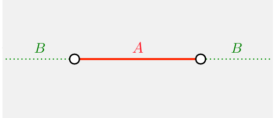
Figure 1: Path integral for reduced density matrix $\rho_{A}$ of an interval of length $\ell$ embedded in an infinite system: The rows and columns of the density matrix are labelled by the values of the fields on the upper and lower edges of the slit along $A$. The field theory expectation value is made finite by eliminating two circular regions of radius $\epsilon$ at the two boundary points (entangling surface) with conformally invariant boundary conditions. The moments ${\rm Tr}\rho_{A}^{n}$ are computed by joining cyclically, along $A$, $n$ replicas of $\rho_{A}$, thus leaving small holes at the entangling surface. The resulting manifold has the topology of an annulus.

In this section we show how the entanglement spectrum distribution in a $1+1$ dimensional conformal field theory [20] can be obtained from the CFT density of states. In fact, we will show that the entanglement spectrum distribution is just a reparametrisation of the former. The main tool to obtain this result is the universal form for the CFT entanglement hamiltonian which has been recently found in [42]. The leading term of the density of states for asymptotically large energies is the famous Cardy formula [48], which during the years has been investigated by many authors in order to include subleading terms [49, 53, 54, 55].

As explained in the introduction, the reduced density matrix can be always written as

$$\rho_{A}=\,e^{-2\pi K_{A}},$$ (18)

where $K_{A}$ is the entanglement hamiltonian. For a 1+1 dimensional CFTs, in the case when $A$ is a finite interval of length $\ell$ embedded in an infinite system, $\rho_{A}$ is given by a path integral which is pictorially reproduced in Fig. 1. The rows and columns of the density matrix are labelled by the values of the fields on the upper and lower edges of the slit along $A$, while along $B$ the field is continuous. In any field theory, this representation of the reduced density matrix is plagued by ultraviolet divergences originated by the degrees of freedom in the vicinity of the boundary points between $A$ and $B$ (generally the boundary between $A$ and $B$ is called entangling surface and we will use this terminology, although in the case of interest here the surface is just made of one or two points). In a CFT, a very convenient way of regularising these ultraviolet divergencies is to remove small disks of radius $\epsilon$ (the ultraviolet cutoff) around the endpoints of the interval [56, 57] (see Fig. 1). The price to pay is that some conformal invariant boundary conditions must be imposed on these disks. At this point, the spacetime in Fig. 1 has the topology of an annulus. Indeed, the mapping between this spacetime and the annulus can be explicitly worked out and the resulting width $W$ of the annulus is related to $\ell$ as $W=2\ln(\ell/\epsilon)+O(\epsilon)$ [56, 42]. An unexpected and surprising result is that the boundary conditions imposed at the small disks affect the value of physical quantities. In particular the Rényi entanglement entropies are [42]

$$S_{n}=\frac{c}{6}\left(1+\frac{1}{n}\right)\ln\frac{\ell}{\epsilon}+\ln g,$$ (19)

where the first term is the well known universal leading logarithmic term [56, 26] and $\ln g$ is the Affleck-Ludwig boundary entropy corresponding to the boundary conditions on the small disks. This should be regarded as surprising because the ultraviolet regularisation of the theory appears to affect physical observables. The explanation for this fact is that there is some physics at the entangling surface (see also [57]): the idea we have in mind is that in a given microscopical model whose low-energy physics is described by a CFT, the partial trace over $B$ induces boundary conditions (which could depend on the actual degeneracy of the ground-state of the model that could not be unique as in a bulk CFT) and these affect physical quantities as in (19). We stress that the $\ln g$ terms (19) is not the same as the one found in [26] which was instead due to the boundary entropy of the physical boundary of a CFT. This is instead analogous to Eq. (9) where $\ln g$ enters as a true degeneration of the entanglement spectrum. The main difference between the two is that in CFT the degeneration $g$ can be non integer.

At this point one could naively think that the actual value of $\ln g$ in a given microscopical model can be always read out from the analysis of the Rényi entropies. This unfortunately is not the case because generically the additive constant term of the entanglement entropy gets non-universal contributions from ultraviolet physics in the bulk which are very difficult to disentangle from the $\ln g$ term. This is evident if one tries to extract $\ln g$ from some analytically known cases, as e.g. those in Refs. [58, 59, 60, 61, 62] and becomes even more cumbersome in numerics. (Anyhow, there are some cases when instead the appearance of $\ln g$ is clear and these will be considered in the next sections to substantiate some of our findings in this section.) One of the consequence of the following analysis is that the actual value of $g$ should be accessible in a easier manner from the analytic or numerical study of the entanglement spectrum distribution.

After this long discussion, we are ready to relate the CFT density of states and the entanglement spectrum distribution. In Ref. [42] the entanglement hamiltonian has been related to the generator of the translations around an annulus with the same conformally invariant boundary condition imposed on the boundaries of the small disks. By exploiting known results on the annulus, the eigenvalues $\kappa_{\Delta}$ of $K_{A}$ have been written as [42]

$$\kappa_{\Delta}=\frac{\pi}{W}\left(\Delta-\frac{c}{24}\right)+\textrm{const},$$ (20)

where $\Delta$ are the conformal dimensions of the operators of the CFT (both the primaries and their descendants). Eq. (20) implies that the eigenvalues $\lambda_{\Delta}$ of $\rho_{A}$ are in one to one correspondence with the spectrum of operators of the CFT as

$$\lambda_{\Delta}=\,e^{-2\pi\kappa_{\Delta}}=\,\lambda_{0}\,e^{-2\pi^{2}(\Delta-c/24)/W},$$ (21)

where the constant in (20) has been absorbed in $\lambda_{0}$. To fix the constant $\lambda_{0}$, let us consider the maximum eigenvalue $\lambda_{\rm max}$ of the RDM, which is obtained for the minimum value of $\Delta$ denoted by $\Delta_{\rm min}$:

$$\lambda_{\Delta_{\rm min}}=\,\lambda_{0}\,e^{-2\pi^{2}(\Delta_{\rm min}-c/24)/W}\;\stackrel{{\scriptstyle W\gg 1}}{{\longrightarrow}}\;\lambda_{0}\qquad\Longrightarrow\qquad\lambda_{0}=\lambda_{\rm max},$$ (22)

i.e., the normalisation constant $\lambda_{0}$, in the limit of large $\ell$, is nothing but the largest eigenvalue of the RDM.

In the limit of large but finite $\ell$ (or equivalently, large $W$), the eigenvalues of the RDM form a continuum and their asymptotic distribution has been determined analytically in [20]. In this manuscript we reobtain this result by using the Cardy formula [48]. Our analysis allows to find that the entanglement spectrum distribution depends also on the Affleck-Ludwig ground state degeneracy [49] which originates from the conformally invariant boundary states characterising the CFT on the annulus. This important feature has been overlooked in all the literature about the entanglement spectrum.

As first step, let us write down explicitly the inverse function $\Delta=\Delta(\lambda)$. From (21) we find

$$\Delta-\frac{c}{24}\,=\,\frac{W}{2\pi^{2}}\,\ln(\lambda_{\rm max}/\lambda_{\Delta})\,=\,\frac{6b}{\pi^{2}c}\,\ln(\lambda_{\rm max}/\lambda_{\Delta}),$$ (23)

where, as in Ref. [20], we have introduced the parameter $b$ as $b\equiv{cW}/{12}=-\ln\lambda_{\rm max}$. Actually, since we are considering the limit of large $\Delta$, the factor $c/24$ is a subleading correction, which we keep since it does not influence the final result.

Given the correspondence (21) between the eigenvalues of the RDM and the conformal spectrum, the distribution of eigenvalues $P(\lambda)$ of the RDM is

$$P(\lambda) = \int_{\Delta_{\rm min}}^{\infty}\rho(\Delta)\,\delta(\lambda-\lambda_{\Delta})\,d\Delta\;=\;\int_{\lambda_{\rm max}}^{0}\rho(\Delta)\,\delta(\lambda-\lambda_{\Delta})\,\frac{d\Delta}{d\lambda_{\Delta}}\,d\lambda_{\Delta}$$ (24)

$$= -\theta(\lambda_{\rm max}-\lambda)\,\frac{d\Delta(\lambda)}{d\lambda}\,\rho(\Delta(\lambda)),$$

where $\rho(\Delta)$ is the density of states in the CFT. This was introduced by Cardy [48] who derived for the first time its large $\Delta$ behaviour for a bulk CFT, known nowadays as the Cardy formula.

In the A we have employed the modular invariance on the annulus to obtain a suitable expression of $\rho(\Delta)$ for large $\Delta$. In order to have a straightforward comparison with [20], we have to take into account also higher order terms in the expansion (see [55] for a similar calculation on the torus). The result reads (see (A))

$$\rho(\Delta)\simeq g\,\frac{\pi^{2}c}{3}\;\frac{I_{1}(\sigma(\Delta))}{\sigma(\Delta)}+g\delta(c-\Delta/24),\qquad{\rm with}\quad\sigma(\Delta)\,\equiv\,2\pi\sqrt{\frac{c}{6}\left(\Delta-\frac{c}{24}\right)},$$ (25)

where $I_{1}$ is the modified Bessel function of the first kind, $c$ is the central charge of the underlying CFT and $g\equiv g_{a}g_{b}$ is the ground-state degeneracy induced by the non-trivial boundary conditions (which in a CFT can be non-integer). Here, $g_{a}\equiv\langle 0|a\rangle$ and $g_{b}\equiv\langle 0|b\rangle$ are the degeneracies introduced by the two boundaries of the annulus. In the case of interest $g_{a}=g_{b}$. Exponentially suppressed contributions have been neglected in (25). By expanding (25) for large $\Delta$ and taking the first subleasing correction after the leading exponential term, the result of [49] is recovered (see (72)).

Eq. (23) allows to write the function $\sigma(\Delta)$ in (25) as function of $\lambda$, obtaining

$$\sigma(\lambda)=\sigma(\Delta(\lambda))=2\sqrt{b\ln(\lambda_{\rm max}/\lambda)}\,,$$ (26)

with $b=-\ln\lambda_{\rm max}$. Finally, plugging the Cardy formula (25) for the density of states, in the distribution of the eigenvalues of the RDM (24) we have

$$P(\lambda)\, = \,\theta(\lambda_{\rm max}-\lambda)\,\frac{6b}{\pi^{2}c\,\lambda}\left[\,g\,\frac{\pi^{2}c}{3}\;\frac{I_{1}(\sigma(\lambda))}{\sigma(\lambda)}\,\right]+g\delta(\lambda-\lambda_{\rm max})$$ (27)

$$= \,\theta(\lambda_{\rm max}-\lambda)\;g\,\frac{b}{\lambda}\,\frac{I_{1}\big{(}2\sqrt{b\ln(\lambda_{\rm max}/\lambda)}\big{)}}{\sqrt{b\ln(\lambda_{\rm max}/\lambda)}}+g\delta(\lambda-\lambda_{\rm max})\,,$$

which is exactly the same as the entanglement spectrum distribution of [20] multiplied by $g$. Denoting by $P_{\mu}(\mu)$ the above distribution for $g=1$ and with $P_{\lambda}(\lambda)$ the one for arbitrary $g$, we have that Eq. (27) satisfies the relation (14) –found for integer $g$– in the limit $-\ln\lambda_{\rm max}\gg 1$. Eq. (27) generalises then the result of the previous section to the Affleck and Ludwig non integer degeneracy [49], showing that it influences the entanglement spectrum distribution in a sensible way. However, in the present case, $g$ can be non-integer [49] and Eq. (27) cannot be derived with the elementary methods of the previous section. Overall, the net effect of the (non-integer) entanglement spectrum degeneracy in CFT is the same found in the previous section for integer degeneracy. In particular the number distribution in CFT is, alike Eq. (17), given by

$$n(\lambda)=gI_{0}(\xi_{\lambda})\,.$$ (28)

We mention that Eqs. (27) and (28) are valid also for the case of a finite system of length $L$ with periodic boundary conditions. Indeed in this case, the worldsheet for $\rho_{A}$ can be mapped in the one of Fig. 1 by a conformal map. Thus, the only change will be the width of the annulus which becomes $W=2\ln[(L/\pi\epsilon)\sin(\pi\ell/L)]+O(\epsilon)$, but this only affects the value of $\lambda_{\rm max}$ and not Eq. (27). Finally in B we show how the above results minimally change in the presence of physical boundaries in CFT: the main difference is that there are two boundary entropies which may be different, one corresponding to the boundary entropy of the physical edge and the other being the boundary entropy introduced through the regularisation procedure at the entangling point, as done above.

4 Analytic results for the spin-1/2 XXZ chain

In this section we explore the general results of the previous sections in some integrable spin chains, for which the entanglement spectrum can be accessed exactly. We present explicit results for the gapped XXZ and Ising spin-chains and exploit their scaling behaviour close to quantum critical points. We use gapped spin-chains because the scaling of the moments of the reduced density matrices are identical to the CFT ones close to the quantum critical points and this implies that also the entanglement spectrum must be the same. Furthermore, the entanglement spectrum of these gapped spin-chains is easily handled analytically, as shown in the following, but the same is not true even for the simplest gapless lattice models.

4.1 The anisotropic Heisenberg spin-chain.

We consider here anisotropic Heisenberg spin-chain (XXZ spin chain), which is defined by the Hamiltonian.

$$H_{XXZ}=\sum_{j}\left[\sigma^{x}_{j}\sigma^{x}_{j+1}+\sigma^{y}_{j}\sigma^{y}_{j+1}+\Delta\sigma^{z}_{j}\sigma^{z}_{j+1}\right]\,,$$ (29)

where $\sigma_{i}^{x,y,z}$ are the Pauli matrices and $\Delta$ is the anisotropy. We focus on the gapped and antiferromagnetic regime for $\Delta>1$. At $\Delta=1$ there is a conformal quantum critical point, separating the gapped antiferromagnetic phase from a gapless conformal one. For $\Delta\to 1^{+}$, the correlation length diverges, and the scaling of the moments of $\rho_{A}$ is given by Eq. (2) with $\ell$ replaced by $\xi$ [26, 63, 64]. This is true in the case of a bipartition in two semi-infinite lines, but also for a finite interval, as long as its length $\ell$ is much larger than $\xi$ (for smaller $\ell$ a complicated crossover to the conformal results takes place [65]).

For the case of a bipartition in two semi-infinite lines, the RDM can be written from the corner transfer matrix as [66, 26, 64]

$$\rho_{A}=\frac{e^{-H_{\rm CTM}}}{{\rm Tr}\,e^{-H_{\rm CTM}}}\,,$$ (30)

where $H_{\rm CTM}$ is [66]

$$H_{\rm CTM}=\sum_{j=0,1}^{\infty}\epsilon_{j}\hat{n}_{j}\,,$$ (31)

where $\hat{n}_{j}$ are fermion number operators with eigenvalues $0$ and $1$ and

$$\epsilon_{j}=2j\epsilon,$$ (32)

with

$$\epsilon={\rm arccosh}\Delta\,.$$ (33)

A very important point for our paper is the initial value of $j$ in the sum in (31). Indeed, $j=0$ and $j=1$ correspond to different ground-states of the model. If the sum starts with $j=1$, we are considering the symmetry breaking state (i.e. the one that for $\Delta\to\infty$ converges to the Néel state). In this state, the largest eigenvalue of the RDM is non-degenerate. Conversely, if the sum starts from $j=0$, we are considering the combination Néel plus its translated by one site (usually called anti-Neel); the latter has zero staggered magnetisation and it does not break the $Z_{2}$ symmetry (but does not satisfy cluster decomposition, which is a fundamental property of physical states). In this case, the largest eigenvalue of the RDM is doubly degenerate, and the same is true for all the spectrum, as a consequence of the zero mode with $j=0$.

Following [66, 12, 51], the entanglement spectrum is obtained by filling in all the possible ways the single particle levels $\epsilon_{j}$ in (31) (i.e., setting all $\hat{n}_{j}$ equal either to $0$ or $1$). The resulting eigenvalues of the reduced density matrix, with $n=\sum_{j}j$ (cf. (31)), are

$$\lambda_{n}=\lambda_{0}e^{-2n\epsilon},$$ (34)

(i.e. the logarithm of the eigenvalues, usually called entanglement levels, are equally spaced with spacing $2\epsilon$). The degeneracy of the $n$-th eigenvalue is given by the number of ways of obtaining $n$ as a sum of smaller non-repeated integers. This is the problem of counting the number $q(n)$ of (restricted) partitions of $n$. The number $q(n)$ is conveniently generated as a function of $n$ via the generating function

$$G(z)\equiv\sum_{k=0}^{\infty}q(k)z^{k}=\prod_{k=1}^{\infty}\left(1+z^{k}\right).$$ (35)

Thus, $q(n)$ is obtained from (35) as the coefficient of the monomial $z^{n}$. The degeneracy of the entanglement spectrum is given either by $q(n)$ or by $2q(n)$ depending on whether we are considering the symmetry breaking state or the symmetric one. This degeneracy of the entanglement spectrum can be written in a compact way as

$${\rm deg}(\lambda_{n})=\gamma q(n),$$ (36)

with $\gamma=1$ or $\gamma=2$ depending on the considered ground-state. The constant $\lambda_{0}$ in (34) is the largest eigenvalue of the RDM and can be simply fixed by the normalisation condition

$${\rm Tr}\rho_{A}=1=\sum_{n}\gamma q(n)\lambda_{0}e^{-2n\epsilon}=\lambda_{0}\,\gamma G(e^{-2\epsilon})\,\qquad\Longrightarrow\qquad\lambda_{0}=\frac{1}{\gamma G(e^{-2\epsilon})}.$$ (37)

Having obtained the analytical expression for the eigenvalues of the RDM and their degeneracies, it is now straightforward to write both entanglement entropies and distribution function of eigenvalues. For example, the moments are

$${\rm Tr}\rho_{A}^{n}=\sum_{k=0}^{\infty}\gamma q(k)\lambda_{0}^{n}e^{-2nk\epsilon}=\lambda_{0}^{n}\gamma G(e^{-2n\epsilon})=\gamma^{1-n}\frac{G(e^{-2n\epsilon})}{(G(e^{-2\epsilon}))^{n}}.$$ (38)

Notice the occurrence of the factor $\gamma^{1-n}$, in agreement with (7).

Let us now move to the number distribution function $n(\lambda)$, i.e. the number of eigenvalues of the RDM larger than $\lambda$. By definition this is nothing but the sum of the degeneracies ${\rm deg}(\lambda_{j})$ of all eigenvalues $\lambda_{j}$ larger than $\lambda$:

$$n(\lambda)=\sum_{\lambda_{j}>\lambda}{\rm deg}(\lambda_{j}),$$ (39)

which using (34) and (36) can be written as

$$n(\lambda)=\sum_{m<\frac{\ln\lambda_{0}/\lambda}{2\epsilon}}\gamma q(m)\,,$$ (40)

which can be straightforwardly evaluated up to very large $j$. Here however, we are interested in the asymptotic behaviour of $n(\lambda)$ which can be obtained by expanding $q(m)$ for large $m$, using Meinardus theorem as in [51] to get

$$q(m)=\frac{1}{4\cdot 3^{1/4}m^{3/4}}\exp(\pi\sqrt{m}/\sqrt{3}).$$ (41)

At this point, the asymptotic behaviour of the number distribution $n(\lambda)$ of the entanglement spectrum for small $\lambda$, i.e., for $\ln\lambda_{0}/\lambda\gg\epsilon$, can be easily calculated integrating (41) to obtain

$$n(\lambda)\simeq\gamma\frac{6^{1/4}e^{\pi\eta/\sqrt{6}}}{2\pi\sqrt{\eta}},$$ (42)

where we introduced the scaling variable

$$\eta\equiv\sqrt{\frac{\ln\lambda_{0}/\lambda}{\epsilon}}\gg 1.$$ (43)

Notice that Eq. (42) is valid for arbitrary $\epsilon$ in the regime when $\eta\gg 1$. Eq. (42) is numerically tested in Fig. 2. The Figure shows the exact result for $n(\lambda)$ obtained using Eq. (40) (symbols in the figure) plotted versus $\eta$. The dash dotted line is (42), and it is in perfect agreement with the exact result for large enough $\eta$.

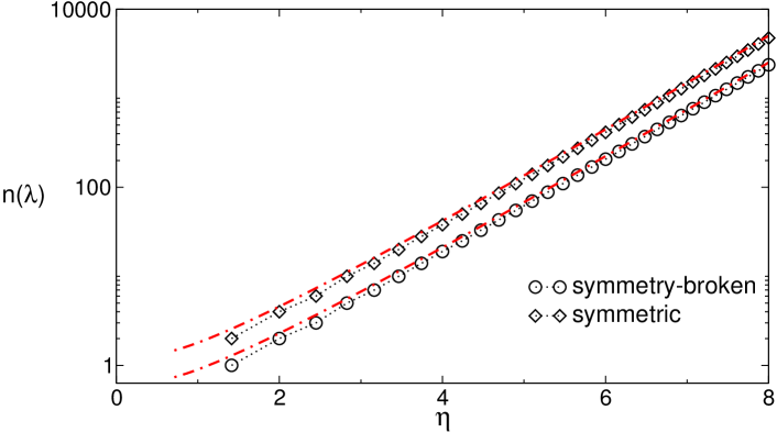
Figure 2: Entanglement spectrum of the XXZ chain in the gapped phase. The number distribution function $n(\lambda)$ is plotted versus $\eta\equiv(\ln(\lambda_{0}/\lambda)/\epsilon)^{1/2}$. The symbols are the exact results in the thermodynamic limit from Eq. (40) while the dashed-dotted lines are the results for large $\eta$ in Eq. (42). The two sets of data correspond to $\gamma=1$ (symmetry-broken) and $\gamma=2$ (symmetric) ground-states.

As already mentioned, $\Delta=1$ corresponds to a quantum critical point with a correlation length diverging as

$$\ln\xi=\frac{\pi^{2}}{2\epsilon}+{\mathcal{O}}(\epsilon^{0}).$$ (44)

Thus for $\Delta\to 1^{+}$, Eq. (42) should match the CFT scaling (28) with the appropriate value of $g$. In order to work out this value of $g$, we can consider the Rényi entropies in the limit $\Delta\to 1^{+}$ (or $\epsilon\to 0$). Eq. (38) can be expanded close to $\epsilon\to 0$ by standard methods [64], obtaining

$$S_{n}=\frac{\pi^{2}}{24\epsilon}\left(1+\frac{1}{n}\right)-\frac{\ln 2}{2}+\ln\gamma+\dots,$$ (45)

where the dots stands for exponentially small terms in $\epsilon$ [64]. We can interpret the $n$-independent additive constant (in $\epsilon$) as the non-integer degeneracy of the ground state of the boundary CFT with the boundary condition induced at the entangling surface. Thus one has

$$g=\frac{\gamma}{\sqrt{2}}\,,$$ (46)

i.e. $g=1/\sqrt{2}$ or $g=\sqrt{2}$ depending on whether $\gamma=1$ or $\gamma=2$.

We now compare the exact result (42) with the expected behaviour from conformal field theory. In the limit $\Delta\to 1^{+}$ (equivalently, $\epsilon\to 0$) the moments of the RDM exhibit conformal scaling. In this limit, taking into account the non-integer degeneracy $g$ of the ground state, the the number distribution function is Eq. (28) with $g$ given in (46), i.e.,

$$n(\lambda)\simeq\gamma I_{0}(\xi_{\lambda})/\sqrt{2}\,,$$ (47)

with $\xi_{\lambda}$ defined in (3). Using $-\ln\lambda_{0}\sim\pi^{2}/24\epsilon+O(1)$ (cf. (45) for $n\to\infty$) one has $\eta\simeq\sqrt{6}\xi_{\lambda}/\pi$ for $\epsilon\to 0$. We then have that, both for $\gamma=1$ and $\gamma=2$, Eq. (42) in the limit $\epsilon\to 1$ coincides with Eq. (47) for large $\xi$, given that $I_{0}(x)\simeq e^{x}/\sqrt{2\pi x}$ for $x\gg 1$. Notice that for the XXZ spin-chain in the regime considered here, the entanglement spectrum distribution function of [20] (i.e. (28) with $g=1$) does not correctly describe the spectrum for none of the two possible ground states.

4.2 The Ising spin-chain in a transverse field

An analysis similar to the one presented in the previous section holds also for the transverse field Ising chain, which is defined by the Hamiltonian

$$H=-\sum\limits_{j=1}^{L}(\sigma_{j}^{x}\sigma_{j+1}^{x}+h\sigma_{j}^{z}),$$ (48)

where $h$ is the external transverse magnetic field. At zero temperature the model is paramagnetic for $h>1$, whereas it is an ordered ferromagnet for $h<1$. At $h=1$ there is a quantum critical point with a low-energy spectrum described by a CFT with $c=1/2$. In the ferromagnetic region, in the limit $L\to\infty$, there are two degenerate ground states, which are related by a $\mathbb{Z}_{2}$ symmetry. In contrast, in the paramagnetic region $h>1$ the ground state is unique.

The entanglement spectrum in both regimes has the same structure (31) as for the XXZ chain, although now the single particle entanglement spectrum levels are given by [66]

$$\epsilon_{j}=\left\{\begin{array}[]{cc}(2j+1)\epsilon&h>1,\\ 2j\epsilon&h<1,\end{array}\right.$$ (49)

with

$$\epsilon\equiv\pi\frac{K(\sqrt{1-k^{2}})}{K(k)},\qquad k\equiv\textrm{min}(h,h^{-1}).$$ (50)

with $K(x)$ the complete elliptic integral of the first kind.

It should be clear that, due to the form of the entanglement levels (49), in the symmetry broken phase for $h<1$ the entanglement spectrum distribution can be derived identically to the previous section. Once again, the distribution depends on whether one considers the symmetric broken or symmetric ground-state, obtained by letting the sum in $j$ starting either from $0$ or $1$. The resulting distribution is then (47) with $\gamma$ given by (46).

In the paramagnetic phase for $h>1$ the entanglement spectrum distribution is instead different from the one of the XXZ model. In this case, the degeneracy of the entanglement spectrum at level $m$ is related from (49) to the number of integer partitions $q_{o}(m)$ of $m$ involving only odd integers (in this case the sum always starts from $j=1$ because the ground-state is unique). The asymptotic behavior for large $m$ of $q_{o}(m)$ is given as 

$$q_{o}(m)\simeq\frac{1}{2\cdot 24^{1/4}m^{3/4}}\exp(\pi\sqrt{m}/\sqrt{6}),$$ (51)

and the corresponding distribution $n(\lambda)$ is

$$n(\lambda)\simeq\frac{6^{1/4}e^{\pi\eta/\sqrt{6}}}{\sqrt{2\eta}\pi}\,,$$ (52)

where, as usual, $\eta\equiv\sqrt{{\ln(\lambda_{0}/\lambda)}/{\epsilon}}\gg 1$. Approaching the critical point at $h=1$, the correlation length diverges as

$$\ln\xi=\frac{\pi^{2}}{\epsilon}+{\mathcal{O}}(\epsilon^{0}),$$ (53)

and the Rényi entanglement entropy as [64]

$$S_{n}=\frac{\pi^{2}}{24\epsilon}\left(1+\frac{1}{n}\right)+O(\epsilon)\,.$$ (54)

Notice in particular the absence of the constant term, suggesting $\ln g=0$. By replacing $\epsilon$ with $\ln\lambda_{0}$ (using (54)), one can straightforwardly show that  (52) coincides with the large $\xi_{\lambda}$ limit of $I_{0}(\xi_{\lambda})$, i.e. (28) with $g=1$.

5 Consequences for the negativity spectrum

The partial transpose $\rho_{A}^{T_{2}}$ of the reduced density matrix is a crucial object for quantifying the bipartite entanglement in a mixed states [69, 70, 71, 72] or, equivalently, the entanglement between two non-complementary parts in a pure state. The partial transpose $\rho_{A}^{T_{2}}$ is defined as $\langle\varphi_{1}\varphi_{2}|\rho^{T_{2}}_{A}|\varphi^{\prime}_{1}\varphi^{\prime}_{2}\rangle\equiv\langle\varphi_{1}\varphi_{2}^{\prime}|\rho_{A}|\varphi^{\prime}_{1}\varphi_{2}\rangle$, with $\{\varphi_{1}\}$ and $\{\varphi_{2}\}$ two bases for $A_{1}$ and $A_{2}$, respectively. A computable measure of entanglement is the logarithmic negativity defined as the sum of the absolute values of the eigenvalues of $\rho_{A}^{T_{2}}$ [71, 72]

$${\cal E}\equiv\ln||\rho_{A}^{T_{2}}||_{1}=\ln\textrm{Tr}|\rho^{T_{2}}_{A}|,$$ (55)

where the symbol $||\cdot||_{1}$ denotes the trace norm. The scaling behaviour of the negativity has been characterised analytically for the ground states of one dimensional CFTs [73, 74, 75]. Remarkably, the negativity is scale invariant at quantum critical points [76, 77, 78, 73]. Its scaling behaviour has been also worked out for finite temperature CFTs [79], in CFTs with large central charge [80], in disordered spin chains [81], in some holographic [86] and massive quantum field theories [87], for out of equilibrium models [82, 83, 84, 85], topologically ordered phases [88, 89], Kondo-like systems [90, 91, 92], and Chern-Simons theories [93, 94]. Surprisingly, no analytical results are available yet for free-fermion models [95], in contrast with free bosonic model, for which the negativity can be calculated [96], also in $d>1$ dimensions [97, 98].

On the same lines as for the entanglement spectrum, it is clear that the partial transpose contains more information than that condensed in the negativity. In analogy with what explained above, part of this information can be reconstructed from the scaling of the moments of the reduced density matrix in a program initiated in [50]. As a fundamental difference compared to the entanglement spectrum, the partial transpose has both positive and negative eigenvalues which generically behave in a different manner. However, their asymptotic CFT distribution for very small eigenvalues turned out to be the same [50].

Here we first focus on the case of a bipartition of the ground state of a CFT, when the spectrum of the partial transpose can be written in terms of the spectrum of the RDM. Although in this case the partially transposed density matrix does not contain more information than the reduced density matrix itself (the two spectra can be simply related [50]), it is very useful to obtain the distribution of these eigenvalues to understand how the CFT non-integer ground-state degeneracy induced at the entangling surface affects the results for the negativity. For this bipartition, the moments of $\rho^{T_{2}}$ can be put in direct relation with those of $\rho_{A_{2}}$ as shown in [73], obtaining

$${\rm Tr}(\rho^{T_{2}})^{n}=\left\{\begin{array}[]{ll}\textrm{Tr}\rho_{A_{1}}^{n_{o}}=c^{T}_{n_{o}}\ell^{-c/6(n_{o}-1/n_{o})}&n_{o}\;\textrm{odd},\\ (\textrm{Tr}\rho_{A_{1}}^{n_{e}/2})^{2}=c^{T}_{n_{e}}\ell^{-c/3(n_{e}/2-2/n_{e})}&n_{e}\;\textrm{even}.\end{array}\right.$$ (56)

The relation between $c^{T}_{n}$ and $c_{n}$ depends on the parity of $n$ and it reads as

$$c^{T}_{n_{o}} = c_{n_{o}},$$

$$c^{T}_{n_{e}} = c_{n_{e}/2}^{2}.$$ (57)

In Ref. [50] the negativity spectrum distribution in CFT has been derived with the assumption $c_{n}=1$ that implies $c^{T}_{n}=1$.

It is now easy to understand the effect of a degeneracy (both integer and non-integer). We have shown that in the presence of degeneracy $g$, cf. Eq. (8), the multiplicative constant $c_{n}$ gets multiplied by $g^{1-n}$, implying a non-trivial relation between the constants $c_{n}^{T}$ for the moments of the partial transpose. According to the equations in (57) we have

$$c_{n_{o}}^{T}(\lambda)=g^{1-n_{o}},$$

$$c_{n_{e}}^{T}(\lambda)=(g^{1-n_{e}/2})^{2}=g^{2-n_{e}}\,.$$ (58)

In [50] it was shown that the number distribution function for the case $c_{n}=1$ is

$$n^{\rm pure}(\lambda)=\frac{1}{2}\big{[}\textrm{sgn}(\lambda)I_{0}(\xi_{\lambda})+I_{0}(2\xi_{\lambda})\big{]},$$ (59)

where $\xi_{\lambda}$ is defined in analogy with Eq. (3) as

$$\xi_{\lambda}=2\sqrt{(-\ln\lambda_{\rm Tmax})\ln(\lambda_{\rm Tmax}/|\lambda|)}\,,$$ (60)

where $\lambda_{\rm Tmax}$ is the maximum positive eigenvalue of the partial transpose (which in the case of a bipartite pure system is equal to $\lambda_{\rm max}$ [50], but not in general). It is easy to check, following the derivation in [50], that the first term comes from the odd moments of the partial transpose, while the second from the even ones.

Thus, to take into account the degeneracy $g$ in (59), the first term gets a factor $g$, whereas the second a factor $g^{2}$. Consequently, in the presence of a global degeneracy $g$, the negativity spectrum distribution is

$$n^{\rm pure}(\lambda)=\frac{1}{2}\big{[}\textrm{sgn}(\lambda)gI_{0}(\xi_{\lambda})+g^{2}I_{0}(2\xi_{\lambda})\big{]}.$$ (61)

This formula is quite interesting because $g$ enters in a different way in the two terms. In particular it shows that for asymptotic small eigenvalues $\lambda$, i.e. large $\xi_{\lambda}$, positive and negative eigenvalues have the same distribution which gets multiplied by $g^{2}$, but the difference of the number distributions (i.e. $n^{\rm pure}(\lambda)-n^{\rm pure}(-\lambda)$) gets multiplied by $g$.

Let us briefly mention what we know about the very interesting case of a tripartite system, when the spectrum of the partially transposed density matrix cannot be written in term of that of the reduced density matrix, because the two intervals are in a mixed state. We focus on the tripartition where two finite intervals $A_{1}$ and $A_{2}$ are adjacent and embedded either in the infinite line or in a finite system. We consider the reduced density matrix $\rho_{A}=\rho_{A_{1}\cup A_{2}}$ and subsequently the partial transpose with respect to $A_{2}$. In this case, the conformal moments of $\rho_{A}^{T_{2}}$ depend on the constants $c_{n}$ appearing in the moments of $\rho_{A_{2}}$ but also on some $n$-dependent structure constants [73, 74]. Assuming that all these parameters are equal to $1$, the negativity spectrum distribution has been obtained in [50] and tested against numerical simulations in spin-chains. In the case when the two intervals have equal length, the final result can be written as [50]

$$n^{\rm mixed}(\lambda)=\frac{1}{2}\big{[}\textrm{sgn}(\lambda)I_{0}(\xi_{\lambda})+I_{0}(\sqrt{2}\xi_{\lambda})\big{]},$$ (62)

where $\xi_{\lambda}$ is defined in Eq. (60) and in this case $\lambda_{\rm Tmax}$ is different from $\lambda_{\rm max}$. Note the $\sqrt{2}$ difference in the argument of $I_{0}$ as compared with (59). At this point, while it is known how the degeneracy factor $g$ affects the multiplicative factors $c_{n}^{T}$, the same is not true for the structure constants and its effect is not trivial. Indeed, for $n=2$ we have ${\rm Tr}(\rho^{T_{2}}_{A})^{2}={\rm Tr}\rho_{A}^{2}$ [74] implying that these structure constants depend on $g$ and we cannot simply set to a constant when $g\neq 1$. In [51], the moments of the partial transpose, as well as the entire negativity spectrum have been analytically worked out for the XXZ spin-chain in the gapped regime discussed in the previous section. While the leading behaviour for large correlation length $\xi$ is the same as in CFT for large $\ell$ (providing to two different exponentials in $n(\lambda)$ as in (62)), the subleading terms are different and so not useful to understand what happens for $g\neq 1$ in a CFT. It would be then very interesting to run some numerical simulations in gapless models with $g\neq 1$ to shed some light on this problem.

6 Conclusions

In this paper we established a relation between the entanglement spectrum distribution of conformal field theories (see Ref. [20]) and the CFT density of states described by the Cardy formula [48]. Indeed, we have shown that the entanglement spectrum distribution can be obtained as a re-parametrisation of the Cardy formula. This result allows us to understand the effect of the boundary conditions at the entangling surface on the entanglement spectrum and entropies. In particular, it shows that the multiplicative constant $c_{n}$ in the moments of the reduced density matrix, cf. Eq. (2), is affected by the degeneracies induced by these boundary conditions, although the leading behaviour in $\ell$ of the moments remains the same. We tested our findings against exact calculations of the entanglement spectrum in integrable spin chains. Furthermore our result shows that the Affleck-Ludwig entropy due to the boundary conditions induced at the entangling surface can be measured from the asymptotic behaviour of the entanglement spectrum distribution. This proposal appears to be more practical than the study of the additive constant of the Rényi entropies whose value in microscopical models is generically influenced by the non-universal ultraviolet physics [58, 59, 60, 61, 62].

We also explored the consequences of degeneracies for the negativity spectrum. In contrast with the entanglement spectrum distribution, which is expressed in terms of a single Bessel function, the negativity spectrum is the combination of two Bessel functions. Remarkably, the presence of a global degeneracy in the entanglement spectrum gives rise to different reparametrisation of the two functions.

A consequence of our findings is that the several numerical results already present in the literature [20, 28, 29, 30, 31, 4] about the validity of the CFT results for the entanglement spectrum distribution (3) can be regarded as direct verifications of the Cardy formula, which, instead, has never been checked at the level of the hamiltonian spectrum of microscopic models. The reason why Cardy formula has not been tested from the hamiltonian spectrum is that CFT describes the low-energy spectrum of microscopic models where the dispersion relation is relativistic, while Cardy formula gives the scaling of the CFT spectrum for large energy, where in microscopic models non-relativistic effects become relevant. Conversely, the entanglement spectrum distribution is written only in terms of the ground-state, and a continuum distribution for the eigenvalues is obtained in the limit $\ell\to\infty$.

Appendix A The Cardy formula on the annulus

In this section we report a derivation of the Cardy formula starting from the partition function of a CFT on the annulus. A similar analysis has been done by employing the geometry of the torus in [55, 54] and of the Klein bottle in [99]. The aim of this computation is to show the occurrence of the boundary states of the annulus in the multiplicative factor of the CFT density of states for large scaling dimensions. This factor corresponds to the ground state degeneracy introduced by Affleck and Ludwig [49].

The starting point is the partition function on the annulus of width $W$ [68] written as a sum over the states parametrised by their conformal dimension $\Delta$

$$\mathcal{Z}(q)=q^{-c/24}\sum_{\Delta}\rho(\Delta)\,q^{\Delta},$$ (63)

where $q=e^{-2\pi^{2}/W}$ is the modular parameter. Here $\rho(\Delta)$ is the Cardy density of states which can be formally obtained by inverting the above relation as a complex integral in $q$

$$\rho(\Delta)=\frac{1}{2\pi{\rm i}}\oint_{C_{0}}\frac{dq}{q^{\Delta+1}}\,q^{c/24}\mathcal{Z}(q),$$ (64)

in which $C_{0}$ is an arbitrary closed path which encloses $q=0$.

By employing the modular invariance, the partition function (63) can be written in terms of the dual modular parameter $\tilde{q}=e^{-2W}$ as [48]

$$\mathcal{Z}(q)=\tilde{q}^{-c/24}\sum_{k}\langle a|k\rangle\langle k|b\rangle\,\tilde{q}^{\delta_{k}},$$ (65)

where the sum is now over all allowed scalar bulk operators with dimensions $\delta_{k}$, and $|a\rangle$ and $|b\rangle$ denote the boundary states at the two edges of the annulus. Plugging this into (64) we have

$$\rho(\Delta)=\frac{1}{2\pi{\rm i}}\oint_{C_{0}}\frac{dq}{q^{\Delta+1}}\,q^{c/24}\,\tilde{q}^{-c/24}\sum_{k}\langle a|k\rangle\langle k|b\rangle\,\tilde{q}^{\delta_{k}}.$$ (66)

Let us know change the integration variable as

$$q=e^{-t},\qquad\tilde{q}=e^{-4\pi^{2}/t}.$$ (67)

Choosing $C_{0}$ to be a circumference centred at the origin $q=0$, we have

$$\rho(\Delta) = \sum_{k}\langle a|k\rangle\langle k|b\rangle\,\frac{1}{2\pi{\rm i}}\int^{t_{1}+{\rm i}\pi}_{t_{1}-{\rm i}\pi}dt\,e^{(\Delta-c/24)t}\,e^{(\gamma-\gamma_{k})/t},$$ (68)

where we introduced

$$\gamma\equiv\frac{\pi^{2}c}{6},\qquad\gamma_{k}\equiv 4\pi^{2}\delta_{k}.$$ (69)

Hereafter $\gamma$ must not be confused with the integer degeneracy factor in the main text.

The above equation is an exact representation of the CFT density of states, valid for arbitrary values of $\Delta$, but it is particularly convenient for a large $\Delta$ expansion. Indeed, for large $\Delta$ two main simplifications occurs. First, the integrals are dominated by the saddle points at $t=0$, thus one can extend the integrals on the imaginary axis between $\pm{\rm i}\infty$ instead of $\pm{\rm i}\pi$. In the same spirit, it is reasonable to keep only the term with $k=0$, being the others expected to be exponentially suppressed. Thus one has

$$\rho(\Delta) \simeq \langle a|0\rangle\langle 0|b\rangle\,\frac{1}{2\pi{\rm i}}\int^{t_{1}+{\rm i}\infty}_{t_{1}-{\rm i}\infty}dt\,e^{(\Delta-c/24)t}\,e^{\gamma/t}$$

$$= \langle a|0\rangle\langle 0|b\rangle\left[\delta(\Delta-c/24)+2\gamma\frac{I_{1}\big{(}2\sqrt{\gamma(\Delta-c/24)}\,\big{)}}{2\sqrt{\gamma(\Delta-c/24)}}\right]$$

$$= \langle a|0\rangle\langle 0|b\rangle\left[\delta(\Delta-c/24)+\frac{\pi^{2}c}{3}\;\frac{I_{1}\big{(}2\pi\sqrt{(c/6)(\Delta-c/24)}\,\big{)}}{2\pi\sqrt{(c/6)(\Delta-c/24)}}\right],$$

where $I_{1}$ is modified Bessel function of the first kind that is obtained by the inverse Laplace transform in (A).

This result is employed in Sec. 3 in a crucial way to recover for $g=1$ the result of [20] from the CFT entanglement spectrum found in [42]. The formula (A) exposes the role of the one-point structure constants $\langle 0|a\rangle$ and $\langle 0|b\rangle$ corresponding to the boundary states which characterise the underlying CFT on the annulus. The term $\delta(\Delta-c/24)$ is often neglected in the literature (see however [100]), because it is subleading for large $W$, but we showed it in order to stress the equivalence with the entanglement spectrum [20]. It is fair to mention that a very similar analysis, but in a slightly different context, has been presented also in [101].

We conclude this appendix by reporting the expansion of the density of states (A) for large $\Delta$. When $\Delta\gg 1$, we can use the following asymptotic behaviour of the Bessel functions

$$I_{1}(z)=\frac{e^{z}}{\sqrt{2\pi z}}\left(1-\frac{3}{8\,z}+O(1/z^{2})\right),$$ (71)

to expand (A) as

$$\rho(\Delta)=\langle a|0\rangle\langle 0|b\rangle\,\frac{\sqrt{\gamma}}{\sqrt{\Delta}}\,\frac{e^{2\sqrt{\gamma\Delta}}}{\sqrt{4\pi(\gamma\Delta)^{1/2}}}=\langle a|0\rangle\langle 0|b\rangle\left(\frac{c}{96\Delta^{3}}\right)^{1/4}e^{2\pi\sqrt{c\Delta/6}},$$ (72)

which is the result found in [49].

Appendix B Entanglement spectrum distribution in the presence of boundaries

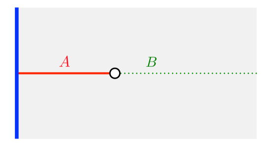
Figure 3: Path integral for reduced density matrix $\rho_{A}$ of an interval of length $\ell$ at the edge of a semi-infinite system whose boundary in the Euclidean spacetime is the solid blue line. The field theory is regularised by removing a small disk of radius $\epsilon$ centred at the point (entangling surface) which separates the interval $A$ from its complement $B$. Conformally invariant boundary conditions which are not necessarily the same are imposed both on the physical boundary (blue solid line) and on the boundary of the small disk (black solid line). The moments ${\rm Tr}\rho_{A}^{n}$ are computed by joining cyclically, along $A$, $n$ replicas of $\rho_{A}$. The resulting manifold is an annulus which can have different conformally invariant boundary conditions at its two boundaries.

In this appendix we discuss how the result for the entanglement spectrum distribution slightly changes in the presence of real boundaries. We focus on the case in which the system is the semi-infinite line $x\geqslant 0$ and the subsystem is the interval $A=[0,\ell]$. The corresponding Euclidean spacetime is the half space $(x,y)\in\mathbb{R}^{2}$ with $x\geqslant 0$, whose boundary is the infinite line $x=0$, which supports a conformally invariant boundary condition of the model. Following the same regularisation procedure adopted in Sec.  3, we remove a small disk of radius $\epsilon$ centred at the entangling point $x=\ell$. A conformally invariant boundary condition is induced along the boundary of this small disk, which may be different from the one along the physical boundary at $x=0$. The resulting spacetime is depicted in Fig. 3. It has the topology of an annulus where different conformally invariant boundary conditions may be present on the physical boundary (blue solid line) and on the boundary of the regularising disk (black solid line). In [42] the latter observation has been employed to study $K_{A}$ for this configuration, finding that for the corresponding entanglement spectrum Eq. (20) holds, but with $W=\log(2\ell/\epsilon)+O(\epsilon)$ in this case.

Thus, the analysis of Sec. 3 can be repeated with the crucial difference that we cannot impose $g_{a}=g_{b}$ because we are allowed to have different conformally invariant boundary conditions. Denoting by $g_{0}$ the degeneracy introduced by the boundary encircling the endpoint $x=\ell$ and by $\tilde{g}$ the degeneracy corresponding to the conformally invariant boundary condition on the physical boundary, for the distribution of eigenvalues we obtain

$$\widetilde{P}(\lambda)=\theta(\lambda_{\rm max}-\lambda)\tilde{g}\,g_{0}\,\frac{b}{\lambda}\,\frac{I_{1}\big{(}2\sqrt{b\ln(\lambda_{\rm max}/\lambda)}\,\big{)}}{\sqrt{b\ln(\lambda_{\rm max}/\lambda)}}+\tilde{g}\,g_{0}\,\delta(\lambda_{\rm max}-\lambda)\,,$$ (73)

being $b=-\ln\lambda_{\rm max}=cW/12=(c/12)\ln(2\ell/\epsilon)+O(\epsilon)$. Integrating (73), the mean number of eigenvalues larger than a given $\lambda$ is simply obtained as

$$\tilde{n}(\lambda)=\tilde{g}g_{0}I_{0}(\xi_{\lambda})\,,$$ (74)

where $\xi_{\lambda}$ is defined in terms of $\lambda_{\rm max}$ in (3).

Eq. (73) is valid also for a finite system of length $L$ with conformal invariant boundary condition at the two ends and with $A=[0,\ell]$. Indeed in this case, the worldsheet for $\rho_{A}$ can be mapped in the one of Fig. 3 by a conformal map. Thus, the only change is the width of the annulus which becomes $W=\ln[(2L/\pi\epsilon)\sin(\pi\ell/L)]+O(\epsilon)$, but this only affects the value of $\lambda_{\rm max}$ and not Eq. (73).

References

References

- [1] L. Amico, R. Fazio, A. Osterloh, and V. Vedral, Entanglement in many-body systems, Rev. Mod. Phys. 80, 517 (2008).
- [2] P. Calabrese, J. Cardy, and B. Doyon Eds, Entanglement entropy in extended quantum systems, J. Phys. A 42 500301 (2009).
- [3] J. Eisert, M. Cramer, and M. B. Plenio, Area laws for the entanglement entropy, Rev. Mod. Phys. 82, 277 (2010).
- [4] N. Laflorencie, Quantum entanglement in condensed matter systems, Phys. Rep. 643, 1 (2016).
- [5] H. Li and F. D. M. Haldane, Entanglement Spectrum as a Generalization of Entanglement Entropy: Identification of Topological Order in Non-Abelian Fractional Quantum Hall Effect States, Phys. Rev. Lett. 101, 010504 (2008).
-
[6]
N. Regnault, B. A. Bernevig, F. D. M. Haldane, Topological Entanglement and Clustering of Jain Hierarchy States,
Phys. Rev. Lett. 103, 016801 (2009);
L. Fidkowski, Entanglement Spectrum of Topological Insulators and Superconductors, Phys. Rev. Lett. 104, 130502 (2010);
A. M. Läuchli, E. J. Bergholtz, J. Suorsa, and M. Haque, Disentangling Entanglement Spectra of Fractional Quantum Hall States on Torus Geometries, Phys. Rev. Lett. 104, 156404 (2010);
N. Regnault and B. A. Bernevig, Fractional Chern Insulator, Phys. Rev. X 1, 021014 (2011). -
[7]
H. Yao and X. L. Qi, Entanglement entropy and entanglement spectrum of the Kitaev model,
Phys. Rev. Lett. 105, 080501 (2010);
F. Pollmann, A. M. Turner, E. Berg, M. Oshikawa, Symmetry protection of topological phases in one-dimensional quantum spin systems, Phys. Rev. B, 81, 064439 (2010);
J. Dubail, and N. Read, Entanglement Spectra of Complex Paired Superfluids, Phys. Rev. Lett. 107, 157001 (2011). -
[8]
D. Poilblanc, N. Schuch, D. Perez-Garcia, and J. I. Cirac, Topological and entanglement properties of resonating valence bond wave functions,
Phys. Rev. B 86, 014404 (2012);
L. Cincio and G. Vidal, Characterizing topological order by studying the ground states of an infinite cylinder, Phys. Rev. Lett. 110, 067208 (2013);
B. Bauer, L. Cincio, B. P. Keller, M. Dolfi, G. Vidal, S. Trebst, A. W.W. Ludwig, Chiral spin liquid and emergent anyons in a Kagome lattice Mott insulator, Nature Commun 5, 5137 (2014). -
[9]
D. Poilblanc,
Entanglement Spectra of Quantum Heisenberg Ladders,
Phys. Rev. Lett. 105, 077202 (2010);
A. Chandran, M. Hermanns, N. Regnault, and B. A. Bernevig, Bulk-edge correspondence in entanglement spectra, Phys. Rev. B 84, 205136 (2011);
X. L. Qi, H. Katsura, and A. W. W. Ludwig, General Relationship Between the Entanglement Spectrum and the Edge State Spectrum of Topological Quantum States, Phys. Rev. Lett. 108, 196402 (2012);
J. Dubail, N. Read, and E. H. Rezayi, Real-space entanglement spectrum of quantum Hall systems, Phys. Rev. B 85, 115321 (2012);
Ivan D. Rodriguez, Simon C. Davenport, Steven H. Simon, and J.K. Slingerland, Entanglement Spectrum of Composite Fermion States in Real Space, Phys. Rev. B 88, 155307 (2013);
G. Y. Cho, K. Shiozaki, S. Ryu, and A. W.W. Ludwig, Relationship between Symmetry Protected Topological Phases and Boundary Conformal Field Theories via the Entanglement Spectrum, arXiv:1606.06402. - [10] M. Hermanns, Entanglement in topological systems, arXiv:1702.01525.
- [11] M. Metlitski and T. Grover, Entanglement Entropy of Systems with Spontaneously Broken Continuous Symmetry, arXiv:1112.5166.
- [12] V. Alba, M. Haque, and A. M. Läuchli, Boundary-locality and perturbative structure of entanglement spectra in gapped systems, Phys. Rev. Lett. 110, 260403 (2013).
- [13] F. Kolley, S. Depenbrock, I. P. McCulloch, U. Schollwöck, and V. Alba, Entanglement spectroscopy of SU(2)-broken phases in two dimensions, Phys. Rev. B 88, 144426 (2013).
- [14] F. Kolley, S. Depenbrock, I. P. McCulloch, U. Schollwöck, and V. Alba, Phase diagram of the J1-J2 Heisenberg model on the kagome lattice, Phys. Rev. B 91, 104418 (2015).
- [15] I. Frérot and T. Roscilde, Entanglement entropy across the superfluid-insulator transition: a signature of bosonic criticality, Phys. Rev. Lett. 116, 190401 (2016).
- [16] M. Fagotti, P. Calabrese, and J. E. Moore, Entanglement spectrum of random-singlet quantum critical points, Phys. Rev. B 83, 045110 (2011).
-
[17]
Z.-C. Yang, C. Chamon, A. Hamma, and E. R. Mucciolo,
Two-component Structure in the Entanglement Spectrum of Highly Excited States,
Phys. Rev. Lett. 115, 267206 (2015);
S. D. Geraedts, R. Nandkishore, N. Regnault, Many body localization and thermalization: insights from the entanglement spectrum, Phys. Rev. B 93, 174202 (2016). - [18] M. Serbyn, A. A. Michailidis, D. A. Abanin, and Z. Papic, Power-Law Entanglement Spectrum in Many-Body Localized Phases, Phys. Rev. Lett. 117, 160601 (2016).
- [19] F. Pietracaprina, G. Parisi, A. Mariano, S. Pascazio, and A. Scardicchio, Entanglement critical length at the many-body localization transition, arXiv:1610.09316.
- [20] P. Calabrese and A. Lefevre, Entanglement spectrum in one-dimensional systems, Phys. Rev A 78, 032329 (2008).
- [21] A. M. Läuchli, Operator content of real-space entanglement spectra at conformal critical points, arXiv:1303.0741.
- [22] R. Lundgren, J. Blair, P. Laurell, N. Regnault, G. A. Fiete, M. Greiter, and R. Thomale Universal entanglement spectra in critical spin chains, Phys. Rev. B 94, 081112 (2016).
- [23] H. Pichler, G. Zhu, A. Seif, P. Zoller, and M. Hafezi, Measurement Protocol for the Entanglement Spectrum of Cold Atoms, Phys. Rev. X 6, 041033 (2016).
- [24] R. Islam, R. Ma, P. M. Preiss, M. E. Tai, A. Lukin, M. Rispoli, and M. Greiner, Measuring entanglement entropy in a quantum many-body system, Nature 528, 77 (2015).
- [25] A. M. Kaufman, M. E. Tai, A. Lukin, M. Rispoli, R. Schittko, P. M. Preiss, and M. Greiner, Quantum thermalization through entanglement in an isolated many-body system, Science 353, 794, 2016.
- [26] P. Calabrese and J. Cardy, Entanglement entropy and quantum field theory, J. Stat. Mech. P06002 (2004).
- [27] P. Calabrese and J. Cardy, Entanglement entropy and conformal field theory, J. Phys. A 42, 504005 (2009).
- [28] F. Pollmann and J. E. Moore, Entanglement spectra of critical and near-critical systems in one dimension, New J. Phys. 12, 025006 (2010).
- [29] V. Alba, M. Haque, and A. M. Läuchli, Entanglement spectrum of the Heisenberg XXZ chain near the ferromagnetic point, J. Stat. Mech., P08011 (2012).
- [30] N. Laflorencie and S. Rachel, Spin-resolved entanglement spectroscopy of critical spin chains and Luttinger liquids, J. Stat. Mech. P11013 (2014).
- [31] R. Susstrunk and D. A. Ivanov, Free fermions on a line: asymptotics of the entanglement entropy and entanglement spectrum from full counting statistics, EPL 100, 60009 (2012).
-
[32]
F. Pollmann, S. Mukerjee, A. Turner, and J. E. Moore,
Theory of finite-entanglement scaling at one-dimensional quantum critical points,
Phys. Rev. Lett. 102, 255701 (2009);
L. Tagliacozzo, T. R. de Oliveira, S. Iblisdir, and J. I. Latorre, Scaling of entanglement support for Matrix Product States, Phys. Rev. B 78, 024410 (2008);
B. Pirvu, G. Vidal, F. Verstraete, and L. Tagliacozzo, Matrix product states for critical spin chains: finite size scaling versus finite entanglement scaling, Phys. Rev. B 86, 075117 (2012). - [33] B. Nienhuis, M. Campostrini, and P. Calabrese, Entanglement, combinatorics and finite-size effects in spin-chains, J. Stat. Mech. (2009) P02063.
- [34] H. Casini and M. Huerta, Reduced density matrix and internal dynamics for multicomponent regions, Class. Quant. Grav. 26, 185005 (2009).
- [35] I. Peschel, and M.-C. Chung, On the relation between entanglement and subsystem Hamiltonians, EPL 96, 50006 (2011).
- [36] H. Casini, M. Huerta and R. Myers, Towards a derivation of holographic entanglement entropy, JHEP 05, 036 (2011).
- [37] A. M. Lauchli and J. Schliemann, Entanglement spectra of coupled spin chains in a ladder geometry, Phys. Rev. B 85, 054403 (2012).
- [38] G. Wong, I. Klich, L. Pando Zayas and D. Vaman, Entanglement Temperature and Entanglement Entropy of Excited States, JHEP 1312 (2013) 020.
- [39] M. Hermanns, Y. Salimi, M. Haque, and L. Fritz, Entanglement spectrum and entanglement Hamiltonian of a Chern insulator with open boundaries, J. Stat. Mech. P10030 (2014).
- [40] D. J. Luitz, N. Laflorencie, and F. Alet, Participation spectroscopy and entanglement Hamiltonian of quantum spin models, J. Stat. Mech. (2014) P08007.
- [41] D. Poilblanc, Entanglement Hamiltonian of the quantum Neel state, J. Stat. Mech. P10026 (2014).
- [42] J. Cardy and E. Tonni, Entanglement hamiltonians in two-dimensional conformal field theory, J. Stat. Mech. (2016) 123103.
- [43] I. Klich, D. Vaman, and G. Wong, Entanglement Hamiltonians for chiral fermions with zero modes, arXiv:1501.00482.
- [44] V. Eisler and I. Peschel, Analytical results for the entanglement Hamiltonian of a free-fermion chain, arXiv:1703.08126.
- [45] I. Klich, D. Vaman, and G. Wong, Entanglement Hamiltonians and entropy in 1+1D chiral fermion systems arXiv:1704.01536.
- [46] M. Dalmonte, B. Vermersch, and P. Zoller, Quantum Simulation and Spectroscopy of Entanglement Hamiltonians, arXiv:1707.04455.
-
[47]
J. Bisognano and E. Wichmann, On the duality condition for quantum fields,
J. Math. Phys. 17, 303 (1976);
J. Bisognano and E. Wichmann, On the Duality Condition for a Hermitian Scalar Field, J. Math. Phys. 16, 985 (1975). - [48] J. Cardy, Operator content of two-dimensional conformally invariant theories, Nucl. Phys. B 270 (1986) 186.
- [49] I. Affleck and A. W. W. Ludwig, Universal non-integer “ground-state degeneracy” in critical quantum systems, Phys. Rev. Lett. 67, 161 (1991).
- [50] P. Ruggiero, V. Alba, and P. Calabrese, Negativity spectrum of one-dimensional conformal field theories, Phys. Rev. B 94, 195121 (2016).
- [51] G. Bigan Mbeng, V. Alba, and P. Calabrese, Negativity spectrum in 1D gapped phases of matter, J. Phys. A 50, 194001 (2017).
-
[52]
A. Kitaev and J. Preskill, Topological Entanglement Entropy,
Phys. Rev. Lett. 96, 110404 (2006);
M. Levin and X.-G. Wen, Detecting Topological Order in a Ground State Wave Function, Phys. Rev. Lett. 96, 110405 (2006);
M. Haque, O. Zozulya, and K. Schoutens, Entanglement entropy in fermionic Laughlin states, Phys. Rev. Lett. 98, 060401 (2007). - [53] S. Carlip, What We Don’t Know about BTZ Black Hole Entropy, Class. Quant. Grav. 15 (1998) 3609.
- [54] S. Carlip, Logarithmic Corrections to Black Hole Entropy from the Cardy Formula, Class. Quant. Grav. 17 (2000) 4175.
- [55] F. Loran, M. Sheikh-Jabbari, and M. Vincon, Beyond Logarithmic Corrections to Cardy Formula, JHEP 1101:110 (2011).
- [56] C. Holzhey, F. Larsen, and F. Wilczek, Geometric and renormalized entropy in conformal field theory, Nucl. Phys. B 424, 443 (1994).
- [57] K. Ohmori and Y. Tachikawa, Physics at the entangling surface, J. Stat. Mech P04010 (2015).
- [58] B.-Q. Jin and V.E. Korepin, Quantum Spin Chain, Toeplitz Determinants and the Fisher-Hartwig Conjecture, J. Stat. Phys. 116, 79 (2004).
- [59] F. Igloi and R. Juhasz, Exact relationship between the entanglement entropies of XY and quantum Ising chains, Europhys. Lett. 81, 57003 (2008).
- [60] P. Calabrese and F. H. L. Essler, Universal corrections to scaling for block entanglement in spin-1/2 XX chains, J. Stat. Mech. P08029 (2010).
-
[61]
P. Calabrese, M. Mintchev, and E. Vicari, Entanglement Entropy of One-Dimensional Gases,
Phys. Rev. Lett. 107, 020601 (2011);
P. Calabrese, M. Mintchev, and E. Vicari, The entanglement entropy of one-dimensional systems in continuous and homogeneous space, J. Stat. Mech. P09028 (2011). - [62] J. Dubail, J.-M. Stéphan, J. Viti, P. Calabrese, Conformal field theory for inhomogeneous one-dimensional quantum systems: the example of non-interacting Fermi gases, SciPost Phys. 2, 002 (2017).
- [63] R. Weston, The Entanglement Entropy of Solvable Lattice Models, J. Stat. Mech. L03002 (2006).
- [64] P. Calabrese, J. Cardy, and I. Peschel, Corrections to scaling for block entanglement in massive spin-chains, J. Stat. Mech. P09003 (2010).
-
[65]
J. L. Cardy, O.A. Castro-Alvaredo, and B. Doyon,
Form factors of branch-point twist fields in quantum integrable models and entanglement entropy,
J. Stat. Phys. 130, 129 (2008);
O. A. Castro-Alvaredo and B. Doyon, Bi-partite entanglement entropy in massive 1+1-dimensional quantum field theories, J. Phys. A 42, 504006 (2009). - [66] I. Peschel, M. Kaulke, and O. Legeza, Density-matrix spectra for integrable models, Ann. Physik (Leipzig) 8, 153 (1999).
- [67] R. J. Baxter, Exactly Solved Models in Statistical Mechanics, 1982 Academic Press, San Diego.
- [68] J. Cardy, Boundary Conditions, Fusion Rules and the Verlinde Formula, Nucl. Phys. B 324 (1989) 581.
- [69] A. Peres, Separability Criterion for Density Matrices, Phys. Rev. Lett. 77, 1413 (1996).
-
[70]
K Zyczkowski, P. Horodecki, A. Sanpera, and M. Lewenstein, On the volume of the set of mixed entangled states,
Phys. Rev. A 58, 883 (1998);
K. Zyczkowski, Volume of the set of separable states. II, Phys. Rev. A 60, 3496 (1999);
J. Eisert and M. B. Plenio, A comparison of entanglement measures, J. Mod. Opt. 46, 145 (1999). - [71] G. Vidal and R. F. Werner, A computable measure of entanglement, Phys. Rev. A 65, 032314 (2002).
-
[72]
M. B. Plenio, The logarithmic negativity: A full entanglement monotone that is not convex,
Phys. Rev. Lett. 95, 090503 (2005);
J. Eisert, Entanglement in quantum information theory, quant-ph/0610253. - [73] P. Calabrese, J. Cardy, and E. Tonni, Entanglement negativity in quantum field theory, Phys. Rev. Lett. 109, 130502 (2012)
- [74] P. Calabrese, J. Cardy, and E. Tonni, Entanglement negativity in extended systems: a quantum field theory approach, J. Stat. Mech. P02008 (2013).
- [75] P. Calabrese, L. Tagliacozzo, and E. Tonni, Entanglement negativity in the critical Ising chain, J. Stat. Mech. (2013) P05002.
- [76] H. Wichterich, J. Molina-Vilaplana, and S. Bose, Scaling of entanglement between separated blocks in spin chains at criticality, Phys. Rev. A 80, 010304 (2009).
- [77] S. Marcovitch, A. Retzker, M. B. Plenio and B. Reznik, Critical and noncritical long range entanglement in the Klein-Gordon field, Phys. Rev. A 80, 012325 (2009).
- [78] H. Wichterich, J. Vidal, and S. Bose, Universality of the negativity in the Lipkin-Meshkov-Glick model, Phys. Rev. A 81, 032311 (2010).
- [79] P. Calabrese, J. Cardy, and E. Tonni, Finite temperature entanglement negativity in conformal field theory, J. Phys. A 48, 015006 (2015).
- [80] M. Kulaxizi, A. Parnachev, and G. Policastro, Conformal Blocks and Negativity at Large Central Charge, JHEP 1409 (2014) 010.
- [81] P. Ruggiero, V. Alba, and P. Calabrese, The entanglement negativity in random spin chains, Phys. Rev. B 94, 035152 (2016).
- [82] A. Coser, E. Tonni and P. Calabrese, Entanglement negativity after a global quantum quench, J. Stat. Mech. P12017 (2014).
- [83] M. Hoogeveen and B. Doyon, Entanglement negativity and entropy in non-equilibrium conformal field theory, Nucl. Phys. B 898, 78 (2015).
- [84] V. Eisler and Z. Zimboras, Entanglement negativity in the harmonic chain out of equilibrium, New J. Phys. 16, 123020 (2014).
- [85] X. Wen, P.-Y. Chang, and S. Ryu, Entanglement negativity after a local quantum quench in conformal field theories, Phys. Rev. B 92, 075109 (2015).
-
[86]
M. Rangamani, and M. Rota, Comments on Entanglement Negativity in Holographic Field Theories,
JHEP 1410 (2014) 060;
E. Perlmutter, M. Rangamani, and M. Rota, Positivity, negativity, and entanglement, Phys. Rev. Lett. 115, 171601 (2015). - [87] O. Blondeau-Fournier, O. Castro-Alvaredo, and B. Doyon, Universal scaling of the logarithmic negativity in massive quantum field theory, J. Phys. A 49, 125401 (2016).
- [88] Y. A. Lee and G. Vidal, Entanglement negativity and topological order, Phys. Rev. A 88, 042318 (2013).
-
[89]
C. Castelnovo, egativity and topological order in the toric code,
Phys. Rev. A 88, 042319 (2013);
C. Castelnovo, Distilling topological entropy from single entanglement measures on projected systems, Phys. Rev. A 89, 042333 (2014). -
[90]
A. Bayat, S. Bose, P. Sodano, and H. Johannesson, Entanglement probe of two-impurity Kondo physics in a spin chain,
Phys. Rev. Lett. 109, 066403 (2012);
A. Bayat, P. Sodano, and S. Bose, Negativity as the Entanglement Measure to Probe the Kondo Regime in the Spin-Chain Kondo Model, Phys. Rev. B 81, 064429 (2010). - [91] A. Bayat, H. Johannesson, S. Bose, and P. Sodano, An order parameter for impurity systems at quantum criticality, Nat. Comm. 5, 3784 (2014).
- [92] B. Alkurtass, A. Bayat, I. Affleck, S. Bose, H. Johannesson, P. Sodano, E. S. Sorensen, and K. Le Hur, Entanglement structure of the two-channel Kondo model, Phys. Rev. B 93, 081106 (2016).
- [93] X. Wen, S. Matsura, and S. Ryu, Edge theory approach to topological entanglement entropy, mutual information, and entanglement negativity in Chern-Simons theories, Phys. Rev. B 93, 245140 (2016).
- [94] X. Wen, P.-Y. Chang, and S. Ryu, Topological entanglement negativity in Chern-Simons theories, JHEP 09 (2016) 012.
-
[95]
V. Eisler and Z. Zimboras, On the partial transpose of fermionic Gaussian states,
New J. Phys. 17 053048 (2015);
A. Coser, E. Tonni, and P. Calabrese, Partial transpose of two disjoint blocks in XY spin chains, J. Stat. Mech. (2015) P08005;
A. Coser, E. Tonni, and P. Calabrese, Towards entanglement negativity of two disjoint intervals for a one dimensional free fermion, J. Stat. Mech. (2016) 033116;
A. Coser, E. Tonni, and P. Calabrese, Spin structures and entanglement of two disjoint intervals in conformal field theories, J. Stat. Mech. (2016) 053109;
P.-Y. Chang and X. Wen, Entanglement negativity in free-fermion systems: An overlap matrix approach, Phys. Rev. B 93, 195140 (2016);
C. P. Herzog and Y. Wang, Estimation for Entanglement Negativity of Free Fermions, J. Stat. Mech. (2016) 073102;
H. Shapourian, K. Shiozaki, and S. Ryu, Partial time-reversal transformation and entanglement negativity in fermionic systems, Phys. Rev. B 95, 165101 (2017);
J. Eisert, V. Eisler, Z. Zimboras, Entanglement negativity bounds for fermionic Gaussian states arXiv:1611.08007. - [96] K. Audenaert, J. Eisert, M. B. Plenio, and R. F. Werner, Entanglement Properties of the Harmonic Chain, Phys. Rev. A 66, 042327 (2002).
- [97] V. Eisler and Z. Zimboras, Entanglement negativity in two-dimensional free lattice models, Phys. Rev. B 93, 115148 (2016).
- [98] C. De Nobili, A. Coser, and E. Tonni, Entanglement negativity in a two dimensional harmonic lattice: Area law and corner contributions, J. Stat. Mech. (2016) 083102.
- [99] H.-H. Tu, Universal entropy of conformal critical points on a Klein bottle, arXiv:1707.05812.
- [100] C. Behan, Density of states in a free CFT and finite volume corrections, Phys. Rev D 88, 026015 (2013).
- [101] K. Najafi and M. Rajabpour, Entanglement entropy after selective measurements in quantum chains, JHEP 1612 (2016) 124.