Decision Theory with a Hilbert Space as Possibility Space

Abstract

In this paper, we propose an interpretation of the Hilbert space method used in quantum theory in the context of decision making under uncertainty. For a clear comparison we will stay as close as possible to the framework of SEU suggested by Savage-1954. We will use the Ellsberg-1961 paradox to illustrate the potential of our approach to deal with well-known paradoxa of decision theory.

Keywords: Decision theory, uncertainty, Ellsberg paradox, quantum theory, Hilbert space, possibility space

JEL Classification codes: C00, C44, D03, D81

1 Introduction

Subjective Expected Utility (SEU) theory (or Bayesian decision theory) in the spirit of Savage-1954 has become the almost uncontested paradigm for decision theory in Economics and Statistics.

In Economics a decision problem is described by a set of states of the world $s\in S$, a set of outcomes (or consequences) $\omega\in\Omega$ and a set of actions $a\in A$. States in $S$ are assumed to be mutually exclusive and to be observed perfectly after realizations, e.g., for a set of states $S:=\{s_{1},s_{2}\}$ state $s_{1}$ could mean ”it rains”’ and state $s_{2}$ ”‘it does not rain”. Outcomes are the ultimate objects which a decision maker values, e.g., sums of money, consumption bundles, work conditions, etc. In this sense, these sets contain semantic information.
In its most general form, actions $a,$ or acts as Savage-1954 calls them, are mappings from states to consequences, $a:S\rightarrow\Omega.$ Hence, the set of potential actions is the set of all such mappings: $A:=\{a|\ a:S\rightarrow\Omega\}.$ A decision maker will choose an action $a$ $\in A$ before knowing which state $s\in S$ will be realized. Once a state $s$ is realized (revealed) the decision maker who chooses action $a$ obtains outcome $a(s).$

According to the behavioristic approach of economics, one assumes that only choices of actions can be observed. Hence, Savage-1954 assumes that every decision maker’s preferences over these actions can be characterized by a complete preference order $\succeq$ on $A.$ A decision maker is assumed to choose $a$ rather than $b$ if and only if $a$ ”is weakly preferred to” $b,\$ $a\succeq b.$

In economic applications, working with objective functions that contain parameters which one can give semantic interpretations simplifies the analysis. Therefore economists have searched for conditions on the preference order $\succeq,$ axioms as Savage-1954 calls them, characterizing an objective function $V:A\rightarrow\mathbb{R}$ which represents preference in the sense that $a\succeq b$ if and only if $V(a)\geq V(b).$

In a seminal contribution, Savage-1954 provides eight axioms on preferences which guaranteed the existence of (i) a utility function $u:\Omega\rightarrow\mathbb{R}$ and (ii) a probability distribution $p$ on $S$ such that the Subjective Expected Utility (SEU) functional $V(a):=\int_{S}u(a(s)\ dp(s)$ represents this preference order $\succeq$. Since the probability distribution $p$ on $S$ is derived from the subjective preferences of the decision maker over action in $A$ it is called a subjective probability distribution.

¿From a normative point of view, the SEU model has become widely accepted as the ”rational” way to deal with decision making under uncertainty. As a descriptive model of behavior, however, the theory has been less successful. Laboratory experiments have confronted decision theory with behavior contradicting the assumption that subjects’ beliefs can be modeled by a subjective probability distribution and that their valuations of random outcomes can be represented by expected utility. Psychological factors have been put forward to explain this phenomenon (e.g., Kahneman-Tversky-1979 *Kahneman-Tversky-1979). Ellsberg-1961 shows that people systematically prefer choices for which information about probabilities is available to uncertain risks. Such behavior violates the basic rules of probability theory.

In response to the Ellsberg paradox and many other discrepancies between behavior observed in laboratory experiments and behavior suggested by SEU theory, Schmeidler-1989 and Gilboa-Schmeidler-1989 started off an extensive literature which tries to accommodate these paradoxes by relaxing the axioms, mostly the independence axiom, proposed by Savage-1954. Machina-Siniscalchi-2014 provide an excellent survey of this literature. All these approaches remain, however, firmly rooted in the Savage framework of states, acts, and consequences.

In this paper, we propose an interpretation of the Hilbert space method used in quantum theory in the context of decision making under uncertainty. This new approach departs from the Savage paradigm of states as ”a description of the world, leaving no relevant aspect undescribed” ( Savage-1954 *Savage-1954, p. 9). In quantum mechanics the state of a system cannot be verified directly in contrast to measurements which can be observed. For the sake of a clear exposition, we will stay in our exposition as close as possible to the framework of SEU suggested by Savage-1954. We will use the two-color urn version of the Ellsberg-1961 paradox to illustrate the potential of our approach to deal with well-known paradoxes of decision theory.

This article illustrates how one can implement an abstract Hilbert space as possibility space in decision theory. We propose mathematical methods common in quantum physics. The difficulties applying quantum mechanics to decision theory come from the distinct terminologies used in both disciplines. Hence, we will pay special attention to concepts in both fields which share names but not meanings. In order to avoid misunderstandings it is necessary to develop a dictionary which relates concepts from decision theory and quantum mechanics. Quantum mechanics uses a mathematical formalism that quantifies possibilities in the form of wave functions. Wave functions are elements of a Hilbert space and represent probability amplitudes. The Hilbert space does not provide probability distributions directly. We will argue in this paper that mapping concepts from quantum mechanics to the theory of decision making under uncertainty promises a framework in which one can deal with the interrelation between subjective beliefs and objective information about events in a non-Bayesian way.

Applying quantum mechanic methods to describe decision making behavior of humans does not mean that ”quantum physics determines human decisions”. Hence, it would be misleading to speak of ”quantum decision theory”. The fact that electromagnetic waves and water waves can be described by the same mathematical methods does not mean that electromagnetic waves consist of water.

Though we hope that our proposed interpretation opens new ways for the analysis of decision making under uncertainty, our focus in this paper is on a suggested interpretation of the quantum mechanics framework in the context of decision theory. Hence, we will not exploit the full power of these methods. It appears, however, straightforward to extend our approach to more general state spaces. Yet, such generalizations will be left for further research.

1.1 Literature

There is a small literature which tries to apply methods of quantum mechanics to decision making in Economics. All these papers use the same mathematical framework of a Hilbert space of wave functions. The main differences lie in the interpretation of the objects of the theory. In particular, one needs to give the ”wave functions” and their entanglement and superpositions an interpretation in an decision context. Moreover, quantum mechanics has no notion of choice over actions or acts. Hence, differences concern mainly these aspects of the theory.

In a series of papers, Diederik Aerts, Sandro Sozzo and Jocelyn Tapia propose a framework for modelling decision making under ambiguity by quantum mechanic methods. Aerts-Sozzo-Tapia-2012 applies a version of this approach to the three-color urn version of the Ellsberg paradox. Similar to the approach suggested in this paper, these authors interpret the elements of a complex Hilbert space as determinants of the probabilities and actions as projectors from the basic elements of the Hilbert space to outcomes or payoffs. In contrast to this paper however, they obtain entanglement by projecting the pre-probabilities of the extreme compositions of the urn.

In a second group of papers, Vyacheslav Yukalov and Didier Sornette model decision making under uncertainty also by a Hilbert space of wave functions. Yukalov-Sornette-2011 apply their model to several paradoxes of decision theory, in particular to an analysis of the disjunction and the conjunction effect. Their interpretation of wave functions as ”intentions” or ”intended actions” is quite different from the interpretation suggested in this paper.

2 Individual decision making and the mathematics of quantum mechanics: a suggested interpretation

In this section, we will describe economic decision in terms of the mathematical concepts provided by quantum mechanics. The most fundamental difference to Savage‘s SEU approach sketched in the introduction is the fact that states of the world are no longer observable after they are realized. In quantum mechanics, ”states of the world” in the Savage sense are orthonormal vectors of a general Hilbert space. General elements of the Hilbert space, which in physics are wave functions, represent states of the world, because they encode all kind of information about the decision context, including probability information about the orthonormal basis states. Most importantly, these states will never be revealed or observed directly. What can be observed however, in a general state are the probabilities of the basis states. These probability distributions over basis states can be obtained by projections of the general state onto the basis states. As we will show in this section, actions will also contain projectors on the basis states.

For simplicity, we choose as starting point a finite dimensional Hilbert space $H:=\mathbb{C}^{|\Omega|}$ spanned by a complete orthonormal set of basis states $\Psi_{\omega}:=|\omega>\in H$. In the following we will use interchangeably the symbols $\Psi$ and the Dirac notation $|\Psi>$ for the elements of the Hilbert space. General states of the world are linear combinations of these basis states $|\beta>=\sum_{\omega=1}^{\Omega}\beta_{\omega}\Psi_{\omega}\in H$. Each state contains several complex amplitudes. Projectors of the composite state on basis states $P_{\omega}:=|\omega><\omega|$ give the probability of finding the basis state $\omega$ in the complex state $|\beta>$. Note, however, that the complex coefficients of a state $|\beta>$ contain more information than probabilities over outcomes.

An action $\alpha$ is a mapping $A_{\alpha}:=\underset{\omega}{\sum}\alpha_{\omega}P_{\omega}$ from composite states to outcome-specific utility payoffs, i.e., a weighted sum of projection operators which map a composite state $|\beta>$ into another state of the Hilbert space $\underset{\omega}{\sum}\alpha_{\omega}P_{\omega}|\beta>$. The average utility $U(\alpha,\beta)$ from an action operator $A_{\alpha}$ in a state $|\beta>\ \in H$ is obtained by evaluating the expectation value of the action in a composite state. In this sense, the state of the world $|\beta>$ allows to identify a probability distribution over outcomes in $\Omega$. The expected utility of action $\alpha$ in the state $|\beta>$ is:

$$U(\alpha,\beta):=<\beta|A_{\alpha}|\beta>=\underset{\omega}{\sum}u(\alpha,\omega)|\beta_{\omega}|^{2}.$$ (1)

For a basis state $|\omega>,$ the action $\alpha$ reveals the utility obtained from the action if the outcome $\omega$ would occur with certainty:
$u(\alpha,\omega):=U(\alpha,\omega)=<\omega|A_{\alpha}|\omega>=\alpha_{\omega}.$

In any state $\beta$, decision makers are assumed to choose among a set of actions $\mathcal{A}$ according to their expected utility $\arg\max\{U(\alpha,\beta)|\ \alpha\in\mathcal{A}\}.$

Remark 2.1

In the ”‘quantum”’ description one has to differentiate clearly between wave functions or vectors and the operators or matrices, It is a linear theory, therefore all operations are simple and do not allow functions of functions.

The following example illustrates this framework.

Example 2.1

Consider an urn containing 100 balls numbered from 1 through to 100. Basis states of the world correspond to situations where a ball with a particular number is drawn from this urn. Hence, the basis states $\Psi_{\omega}$ correspond to states where a ball with a particular number is drawn. General composite states are complex-valued weighted sums of the basis states $|\beta>=\sum_{\omega}\beta_{\omega}\Psi_{\omega}$ and contain information about the relative frequencies of the outcomes. In this case, the Hilbert space $H=\mathbb{C}^{100}.$
Betting 100 Euros on a ball with an even number $\omega$ being drawn from the urn is an action $A_{\alpha^{e}}=\underset{\omega}{\sum}\alpha_{\omega}^{e}P_{\omega}\$with

$$\alpha_{\omega}^{e}=\left\{\begin{tabular}[]{lll}$100$&for&$\omega$ even\\ $0$&for&$\omega$ odd\end{tabular}\ \right..$$

The action $a^{e}$ of betting on an even number induces a utility vector over outcomes yielding in state $|\beta>$ the expected utility

$$U(\alpha^{e},\beta):=<\beta|A_{\alpha^{e}}|\beta>=\underset{\begin{tabular}[]{l}$\omega\in\Omega$\\ $\omega$ even\end{tabular}}{\sum}100|\beta_{\omega}|^{2}.$$ (2)

Similarly, a bet on the odd numbers $P_{\alpha^{o}}=\underset{\omega}{\sum}\alpha_{\omega}^{o}P_{\omega}$ with $\alpha_{\omega}^{o}=\left\{\begin{tabular}[]{lll}$100$&for&$\omega$ odd\\ $0$&for&$\omega$ even\end{tabular}\right.$ yields an expected utility of $U(a^{o},\beta)=<\beta|A_{\alpha^{o}}|\beta>$. We assume that, in a state $\beta,$ a decision maker chooses among actions $\alpha\in\mathcal{A}:=\{\alpha^{e},\alpha^{o}\}$ according to whether $U(\alpha^{e},\beta)\lessgtr U(\alpha^{o},\beta).$

The following table summarizes the basic framework of a decision problem:

$$\bullet$$ Hilbert space

Basis states

(complete set of normalized wave functions )

Composite states of the world

(also normalized)

Probability of an outcome in :

Actions

Payoffs of action

Expected payoff of action in state :

The expected payoff of an action $\alpha\ \$in a composite state $\beta,\ U(\alpha,\beta),$ can be expanded as follows:

$$U(\alpha,\beta) : =<\beta|A_{\alpha}|\beta>=<\beta|\underset{\omega}{\sum}\alpha_{\omega}P_{\omega}|\beta>$$

$$= \underset{\omega}{\sum}\alpha_{\omega}<\beta|P_{\omega}|\beta>=\underset{\omega}{\sum}\alpha_{\omega}|\beta_{\omega}|^{2}.$$

In this framework, an action $\alpha$ assigns payoffs (in terms of utility) to the outcomes of a composite state.

As in Anscombe-Aumann-1963 a state will be associated with a probability distribution over outcomes. In contrast to Anscombe-Aumann-1963, however, we do not assume that states can be observed directly. Instead, the possible states of the world determine the probabilities over outcomes by projection operators whose expectation values give the probabilities of the outcomes. A decision maker’s information about possible probability distributions over outcomes is encoded in the states of the world.

The following example illustrates these concepts in the context of a simple portfolio choice problem.

Example 2.2 (Portfolio choice)

Consider two assets, a stock $a$ and a bond $b.$ The stock pays a state contingent payoff $(r_{1}q_{0},r_{2}q_{0}).$ The bond pays off the same $r$ in each state.

price quantity payoff

state $$1$$ state

stock:

bond:

Basis states are $\Omega=\{1,2\}$ reflecting the per unit return in each state, $r_{1}>r_{2}.$ The Hilbert space $H$ spanned by the two basis states $|1>$ and $|2>$ contains composite states $|\beta>=\beta_{1}|1>+\beta_{2}|2>$ which capture all information available in state $\beta.$ An investor chooses a portfolio $\alpha=(a,b)$ subject to a budget constraint $q_{0}a+b=W_{0},$ where $W_{0}$ denotes the initial wealth of the investor. For an investment $\alpha=(a,b)$ and a state $\beta,$ the investor expects an expected utility of

$$U(\alpha,\beta) = U(\alpha,1)|\beta_{1}|^{2}+U(\alpha,2)|\beta_{2}|^{2}$$

$$= u(r_{1}a+rb)|\beta_{1}|^{2}+u(r_{2}a+rb)|\beta_{2}|^{2}.$$

Given state $\beta,$ a decision maker will choose an action $\alpha^{\ast}$ from a set $\mathcal{A}$ which yields the highest expected utility $U(\alpha,\beta),$ i.e., $U(\alpha^{\ast},\beta)\geq U(\alpha,\beta)$ for all $\alpha\in\mathcal{A}.$ Notice, however, that, in contrast to classical economic decision theory, the optimal choice $\alpha^{\ast}$ will depend on $\beta$ the state which determines the expected utility.

Remark 2.2

Since states $\beta$ in the Hilbert space $H$ cannot be observed directly, observing the action chosen by a decision maker will in general not reveal the state $\beta$ completely.

2.1 Subjective states of mind

The main conceptual contribution of our paper is the assumption that a decision maker’s subjective attitudes towards the available information can be modelled by a subjective state of mind. States of mind are elements of the Hilbert space $H$ which represent subjective information about the environment and the decision makers attitude towards such information. In particular, the subjective state of mind interacts with the actual and potential states of the world. In analogy to to a subjective prior in Bayesian decision making, the subjective state of mind weighs the information contained in the states and assesses their relevance for the choice of actions. Other than a subjective Bayesian prior distribution, however, the notion of a state of mind captures also psychological features of information processing and distortion. A state of mind represents the decision maker’s perception of the uncertainty. As we will explain in detail below, the decision maker’s perception of uncertainty will change in the light of new information. Such information is also encoded in elements of the Hilbert space and will interact with the subjective state of mind. This interaction allows us to use the power of quantum mechanics to model ”entanglements” and ”superpositions”.

Formally, a state of mind $\Psi_{M}$ is a composite state $|M>~{}$in $H.$ It is associated with the projector $P_{M}=|M><M|$ which projects any state $\Psi_{\beta}$ on to $\Psi_{M}$:

$$P_{M}|\Psi_{\beta}>=c_{\beta}|M>.$$ (3)

Suppose a decision maker with a state of mind $\Psi_{M}$ is confronted with information of another state $\Psi_{\beta}.$ Although $\Psi_{\beta}$ represents a normalized state, the moderated state of mind $P_{M}|\Psi_{\beta}>$ is no longer normalized. In general the coefficient $c_{\beta}$ is complex, but the absolute magnitude $|c_{\beta}|$ of the projection can be used as a measure of distance in information of state $|\beta>$ from the subjective ”mind state”. The more distant the state $|\beta>$ is from the mind state $|M>$ the smaller the length of the projection (c.f. Fig.1).

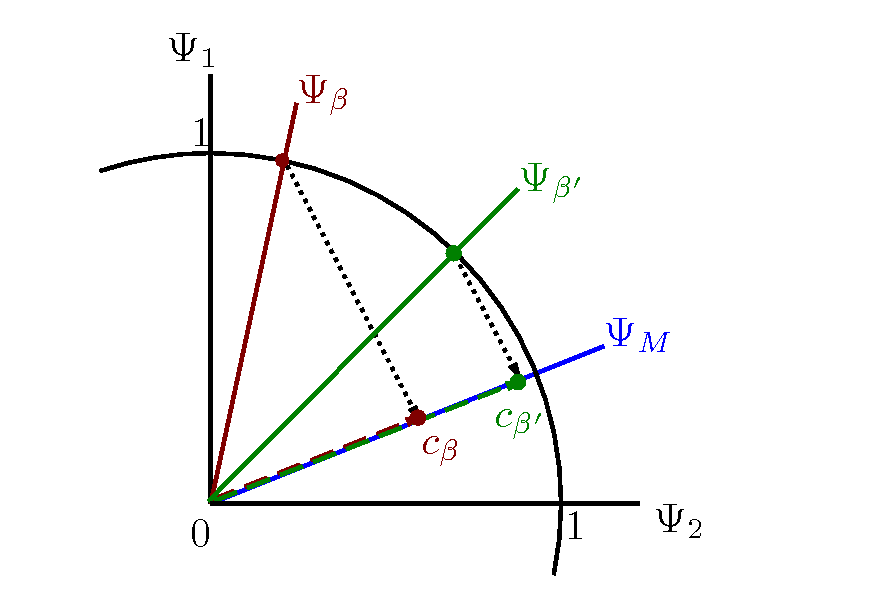
Figure 1: Schematic picture showing the effect of the projection of a composite state on the mind state. The length of the projection indicates its similarity with the mind state (in general, the coefficients $c$ will be complex numbers)

To assess the information about the basis states $|i>$ contained in an arbitrary state of the world when the mind state is present, one evaluates the expected value of the product of the projectors $P_{M}P_{i}P_{M}$. For a composite state $|\Psi_{\beta}>$ one gets:

$$<\beta|P_{M}P_{i}P_{M}|\beta>\ = < \beta|M><M|P_{i}|M><M|\beta>\$$ (4)

$$= |c_{\beta}|^{2}<M|P_{i}|M>$$ (5)

where

$$c_{\beta}=<M|\beta>.$$ (6)

As a result one obtains the probability for the basis state $|i>$ in the mind state $\Psi_{M}$ multiplied with the absolute square of the amplitude $|c_{\beta}|$. The weight $|c_{\beta}|^{2}$ indicates the extent to which the state $|\beta>$ agrees with the mind state $|M>$. For $|\beta>=|M>$ the decision maker’s state of mind will be consistent with the actual state information, $|c_{\beta}|^{2}=1$.

This framework allows us to study how the subjective state of mind $\Psi_{M}$ interacts with actual information. The projections on to the basis states can be interpreted as a core belief and the possible distances $|c_{\beta}|$ as measures of ambiguity regarding the information contained in other states.

In the following section we will illustrate how this general framework can model behavior in the two-state Ellsberg paradox.

3 The Ellsberg experiment

In a seminal paper published in 1961, Ellsberg-1961 suggested the following thought experiment. Consider two urns each containing 100 balls (see Fig.2). The balls are either black or white. It is known that the first urn contains exactly 50 black and 50 white balls. For the second urn however, the composition of the colors is unknown.

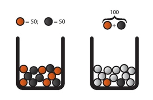
Figure 2: The two Ellsberg urns: Urn 1 on the left contains well defined proportions of black and white balls, whereas for urn 2 on the right the proportions are unknown.

Subjects hold bets on the color of the balls to be drawn from the urns. A bet on black $"b"$ yields $100$ Euro if the ball drawn from the urn is black. Otherwise the payoff is zero. Similarly, betting on white $"w"$, the subject earns $100$ Euro if a white ball is drawn and nothing otherwise. Table 1 summarizes this choice problem.

Urn 1 Urn 2

50 50 100

Black White Black White

$$b$$ (bet on black)

(bet on white)

Holding a bet first on black ($b$) and then on white ($w$), subjects had to choose the urn on which they wanted to bet.

A large number of subjects, about 60 percent, choose to bet on the draw from Urn 1 for both bets. These choices clearly contradict the assumption that these subjects were maximizing SEU.

Denoting by $p_{u}(B)$ the probability of the event $B$ that a black ball is drawn from urn $u$, $u=1,2,$ the expected utilities of a bet on color $B$ from Urn $u$ is $U_{u}(b)=p_{u}(B)u(100)+\left[1-p_{u}(B)\right]u(0)$ and a bet on $W$ from Urn $u$ is $U_{u}(w)=p_{u}(B)u(0)+\left[1-p_{u}(B)\right]u(100).\$Obviously, choosing Urn 1 for both bets leads to a contradiction since

$$\bullet$$ implies

implies

Thus, the assumption of the decision maker maximizing SEU fails. Notice that for this conclusion it does not matter what utilities $u(100)$ and $u(0)$ are attached to outcomes, i.e., independent of risk attitude. We only require $u(100)>u(0)$.

3.1 Modelling the Ellsberg experiment by a Hilbert space

The special feature of the Ellsberg experiment, where subjects face the same bets on the same type of urn, lies in the fact that the information about the composition of the urn is precise in case of Urn 1 and imprecise in case of Urn 2. We interpret this experimental arrangement in such a way that the precision of information is reflected in two mind states of the decision maker, i.e., the two urns exist separately in the imagination of the experimenter. We therefore model them as two mind states in the same Hilbert space.

The basis states $|\omega>$ of the Hilbert space consist of the two exclusive cases (outcomes of the experiment) $\Psi_{W}=|W>,\ i.e.$ ”a white ball is drawn from the urn” and $\Psi_{B}=|B>\$i.e.,  ”a black ball is drawn from the urn” . These basis states are exclusive i.e. orthogonal and normalized, i.e., $<B|W>=<W|B>=0\$and $<B|B>=<W|W>=1$. Composite states $|\beta>=\beta_{B}|B>+\beta_{W}|W>$ of the Hilbert space $H\$spanned by these basis states are characterized by the complex weights $\beta=(\beta_{B},\beta_{W}).$

The information of the decision maker regarding the composition of the urns is encoded in the respective composite states (wave functions) for the different urns. Urn 1, the urn with the known proportion of $\frac{1}{2}$ black and white balls, is described by the composite wave function $\Psi_{1}$

$$\Psi_{1}=\frac{1}{\sqrt{2}}\left(\Psi_{B}+\Psi_{W}\right)$$

and Urn 2, for which the composition is unknown, is described by the wave function $\Psi_{2}(x)$

$$\Psi_{2}(x)=x\Psi_{B}+\sqrt{1-x^{2}}\Psi_{W}$$

Without reducing the generality of our further arguments we can choose $x$ real, any choice of complex phases in $\Psi_{2}$ can be absorbed in the final phase of the mind state.

The parameter $x$ contains the information about the composition of Urn 2. Since it is known that there is a finite number of 100 balls in Urn 2, we assume that the number of possible states $\Psi_{2}(x)$ of the Hilbert space $H$ is finite.

The probabilities of the outcomes, a white ball is drawn from the urn $W$ or a black ball is drawn from the urn $B$, are obtained by the projection operators $P_{\omega}$, the sum of which yields the identity operator:

$$P_{B}=|B><B|,$$ with

The probabilities of the outcomes are the expectation values of these projection operators evaluated with the respective composite state. The expectation values of the projection operators assign probabilities to the outcomes given the information of a specific state of the world, $\Psi_{1}$ or $\Psi_{2}(x)$:

$$\bullet$$ Urn 1: and

Urn 2: and

The two bets are modelled by the operators $A_{B}=u(100)P_{B}+u(0)P_{W}$ and $A_{W}=u(0)P_{B}+u(100)P_{W}$ . Hence, given the information about Urn 1 contained in $\Psi_{1},$ one obtains the following expected utilities from these actions:

$$U(b,1) = <\Psi_{1}|A_{B}|\Psi_{1}>=\frac{1}{2}u(100)+\frac{1}{2}u(0),$$

$$U(w,1) = <\Psi_{1}|A_{W}|\Psi_{1}>=\frac{1}{2}u(0)+\frac{1}{2}u(100).$$

Similarly, given the information regarding Urn 2, one has

$$U(b,x) = <\Psi_{2}(x)|A_{B}|\Psi_{2}(x)>=x^{2}u(100)+\left(1-x^{2}\right)u(0),$$

$$U(w,x) = <\Psi_{2}(x)|A_{W}|\Psi_{2}(x)>=x^{2}u(0)+\left(1-x^{2}\right)u(100).$$

Given this information about the urns and no subjective processing of information, the Ellsberg puzzle would remain unresolved. A choice of betting on Urn 1 in both cases would yield for any $x\in\mathcal{R}$,

$$\bullet$$

3.2 Solution of the paradox: a subjective mind state

Applying the notion of a mind state represents the decision makers assessment of the situation given her information. In case of Urn 2, all the person knows is the total number of balls in the urn. Hence, her mind state is a subjectively determined general state from the Hilbert space $H$

$$\Psi_{M2}(y,d):=y|B>+e^{id}\sqrt{1-y^{2}}|W>$$

which is characterized by the parameters $(y,d).$ In general, different decision makers will have different initial states of mind $\Psi_{M2}(y,d).$

All decision makers are however confronted with the same information about Urn 2

$$\Psi_{2}(x)=x\Psi_{B}+\sqrt{1-x^{2}}\Psi_{W}$$

with the unknown parameter $x\in\mathcal{R}$.

We assume that the mind state $\Psi_{M2}(y,d)$ distorts the perception of the basis states of the world represented by the projectors $P_{\omega}:=|\omega><\omega|,$ $\left(\omega=B,W\right)$, i.e., the operators to draw a black or a white ball,

$$P_{B} \rightarrow P_{M2}P_{B}P_{M2},$$

$$P_{W} \rightarrow P_{M2}P_{W}P_{M2},$$

where

$$P_{M2} = |M2><M2|$$

$$= \left[\begin{array}[]{cc}y^{2}&e^{-id}y\sqrt{1-y^{2}}\\ e^{id}y\sqrt{1-y^{2}}&1-y^{2}\end{array}\right]$$

is the projector of the mind state. For the mind state, the amplitudes reflect the subjective distortions. Hence,

$$\left\langle\Psi_{2}(x)|P_{M2}P_{B}P_{M2}|\Psi_{2}(x)\right\rangle = <\Psi_{2}(x)|M2><M2|P_{B}|M2><M2|\Psi_{2}(x)>$$

$$= y^{2}|c_{x}|^{2}.$$

with

$$y^{2} = <M2|P_{B}|M2>$$

$$|c_{x}|^{2} = |<M2|\Psi_{2}(x)>|^{2}$$

$$= \left(1-x^{2}-y^{2}+2x^{2}y^{2}+2xy\sqrt{(1-x^{2})(1-y^{2})}\cos{d}\right)$$

One sees how the mind state overwrites the state $\Psi_{2}(x)$ of Urn 2, and modifies the resulting probability with the overlap probability of the two states. This overlap probability contains an interference term which is visible from the trigonometric function. It encodes the reliability the person assigns to his/her estimate of this probability. Similarly, one obtains the probability of $W$ from the distorted state as

$$\left\langle\Psi_{2}(x)|P_{M2}P_{W}P_{M2}|\Psi_{2}(x)\right\rangle = <\Psi_{2}(x)|M2><M2|P_{W}|M2><M2|\Psi_{2}(x)>$$

$$= (1-y^{2})|c_{x}|^{2}.$$

with $|c_{x}|^{2}$ as above and

$$1-y^{2} = <M2|P_{W}|M2>$$

In the case of Urn 1, the decision maker knows the composition of the urn. Hence, her mind state should be one of subjective certainty

$$|\Psi_{M1}>=|\Psi_{1}>=\frac{1}{\sqrt{2}}\left(\Psi_{B}+\Psi_{W}\right)$$

where the state of mind $|\Psi_{M1}>$ coincides with the actual information $|\Psi_{1}>$.

Hence, we have

$$<\Psi_{1}|P_{M1}P_{\omega}P_{M1}|\Psi_{1}>=|<\Psi_{M1}|\Psi_{1}>|^{2}<\Psi_{M1}|P_{\omega}|\Psi_{M1}>=\frac{1}{2}$$

for $\omega=W$ and for $\omega=B.$

Given the action projectors of the two bets $A_{B}=u(100)P_{B}+u(0)P_{W}$ and $A_{W}=u(0)P_{B}+u(100)P_{W},$ one obtains as the conditions for Ellsberg behavior:

• for the bet on Black $b,$ Urn 1 is preferred if

  $$U(b,1,M1)>U(b,x,M2)$$

  with

  $$U(b,1,M1) = \left\langle\Psi_{1}|P_{M1}A_{B}P_{M1}|\Psi_{1}\right\rangle$$

  $$= \frac{1}{2}\left[u(100)+u(0)\right],$$

  $$U(b,x,M2) = |c_{x}|^{2}\left[y^{2}u(100)+\left(1-y^{2}\right)u(0)\right],$$

• for a bet on White $w,$ Urn 1 is preferred if

  $$U(w,1,M1)>U(w,x,M2)$$

  with

  $$U(w,1,M1) = \left\langle\Psi_{1}|P_{M1}A_{W}P_{M1}|\Psi_{1}\right\rangle$$

  $$= \frac{1}{2}\left[u(100)+u(0)\right],$$

  $$U(w,x,M2) = |c_{x}|^{2}\left[y^{2}u(0)+\left(1-y^{2}\right)u(100)\right].$$

For $u(0)=0$ and $u(100)=1,$ we obtain the following conditions:

$$\frac{1}{2} > |c_{x}|^{2}y^{2},$$

$$\frac{1}{2} > |c_{x}|^{2}\left(1-y^{2}\right).$$

Assuming no effect of the interference term $d=\frac{\pi}{2},$ i.e., $\cos{d=0,}$ Fig.3 shows the regions for the Ellsberg choices.

Figure 3: The figure shows for fixed $d=\frac{\pi}{2}$ the region $\frac{1}{2}>|c_{x}|^{2}y^{2}$ and $\frac{1}{2}>|c_{x}|^{2}\left(1-y^{2}\right)$ as grey ( in color blue) shaded area.

On the horizontal axis we consider values of $x\in[0,1]$ and on the vertical axis of $y\in[0,1].$ In this diagram we consider the case without interference due to the complex conjugate since $d=\frac{\pi}{2}\$implies$\ \cos{d=0.}$ In this case, $|c_{x}|^{2}$ simplifies to $\left(1-x^{2}-y^{2}+2x^{2}y^{2}\right).$ The grey ( in color blue) area contains $(x,y)$ combinations which correspond to Ellsberg behavior. Integrating, one obtains an area of approximately 63 percent. In our interpretation, the parameter $y$ captures the decision maker’s initial disposition in regard to Urn 2. The parameter $x,$ which is measured as the unknown actual probability of the draw of a black ball, captures the objective circumstances of the situation. Projecting $\left(x,\sqrt{1-x^{2}}\right)$ onto the mind state $\left(y,e^{\frac{\pi}{2}i}\sqrt{1-y^{2}}\right)$ yields a mind state which is affected by the actual situation.

In their review of 39 experimental studies of the Ellsberg paradox, Oechssler-Roomets-2015 find a wide range of measured ambiguity across the various studies. These different experimental contexts which include the different ways of actually choosing the proportion on the balls in the unknown urn reflects the kind of objective experimental environment which meets the individual states of minds of the subjects. The resulting behavior is influenced by both factors, the subjective mind state $y$ and the objective situation $x.$ Measurements such as the observed behavior and the stated predictions regarding the proportions of the colors should reflect these parameters. This will be discussed in the next section.

4 Discussion and Conclusion

The Ellsberg paradox (Ellsberg-1961) is usually interpreted as a manifestation of the decision maker’s ambiguity about the unknown proportions in Urn 2. Faced with a choice between bets on draws from an urn with a known probability distribution and bets on an urn with an unknown probability distribution people prefer to bet on draws from the urn with the known probability distribution. In the two urn problem individual subjects select for all bets the urn where white and a black balls are equally distributed. Such behavior is inconsistent with maximization of expected utility for any subjective probability distribution regarding the composition of Urn 2. In the literature on decision making under uncertainty, most of the suggested solutions of the paradox assume ”ambiguity aversion” of the decision maker, i.e., the decision maker evaluates bets on Urn 2 according to the worst case of all possible compositions.

The model which we put forward in this paper goes beyond this psychological explanation by ”pessimism” and invokes the framework of a Hilbert space as possibility space which captures various aspects of the choice situation including, but not being confined to, information about the composition of the urns. The Hilbert space contains the two possible draws from the urns, a black ball or a white ball, as basis states. Based on the information about the urns, one constructs wave functions for the respective urn states from these basis states. These wave functions may contain complex amplitudes entangling the basis states. Hence, there is more information in these wave functions than in real probabilities.

In applications to a decision-theoretic context, a crucial role is played by the subjective mind states which reflect the mental perception (consciousness) of the subjects in the experiment. The precise information about the content of Urn 1 we represent by a mind state equal to a preprobability without complex amplitude. For the second urn, however, the mind state represents other possibilities than the one given by the unknown objective composition of the second urn. In this case the parameters describe the influence of beliefs, information, and other context variables on the state of the second urn. The single complex phase in the mind state summarizes all possible effects of complex amplitudes for the second-urn wave functions.

For the three parameters $(x,y,d)$, the condition for choices corresponding to the typical Ellsberg behavior defines a subspace of the feasible space of the three parameters. Fig. 4 illustrates the entanglement due to the complex amplitude for the parameter space of our model $[0,1]\times[0,1]\times[0,\pi]$.

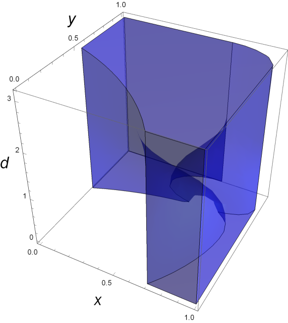
Figure 4: The figure shows the grey (in color blue) region in the three parameter space of $x,y,d$ connected to the objective and subjective second urn state with $\frac{1}{2}>|c_{x}|^{2}y^{2}$ and $\frac{1}{2}>|c_{x}|^{2}\left(1-y^{2}\right)$

In a first attempt to summarize the results about ambiguity-averse behavior across the 39 Ellsberg experiments in their review, Oechssler-Roomets-2015 obtain an average ratio $\ r_{emp}$ of approximately 57 percent ambiguity averse subjects,

$$r_{emp}\in[57.2\%,57.9\%].$$

Using the ratio of the volume of the subspace of parameters leading to ambiguity-averse choices to the total volume as a naive measure for the percentage of ambiguity averse decisions in the Ellsberg two-urn problem yields the ratio $r_{quant},$

$$r_{quant}=58.1\%\pm 0.5\%.$$

Though one obtains a surprisingly similar proportion, we do not claim that aggregating over all parameter values is an appropriate measure for ambiguity averse behavior in our model. A more careful analysis may restrict the range of reasonable mind states and their complex amplitude $(y,d)$.

The Hilbert space method which we suggest in this paper increases the number of parameters in general. On the one hand, this allows us to explain results which are paradoxical in classical decision theory, on the other hand, this exposes the model to the danger of arbitrariness. In especially designed experiments, however, one could ask more questions in order to study the role of these additional parameters separately. E.g., in the two urn problem one could ask the subjects for their estimate of the number of black and white balls in the second urn. This would allow one to fix one of the parameters of the wave function of the mind state, thus providing a more stringent test of the model.

In Economics and most of the Social Sciences, classical decision theory under uncertainty in the framework of Savage-1954 has been extremely fruitful, allowing economists to develop new fields such as information economics, contract theory, and financial markets analysis. Human choice behavior as observed in experiments, however, has cast some doubts on the general accuracy of the Savage approach as a description of actual behavior. Yet most existing generalizations of the SEU model maintain the basic framework of actions mapping states into consequences.

The main conceptual difference between the Savage framework and the Hilbert space approach advanced in quantum mechanics is the notion of a ”state”. Savage-1954  defines ”a state (of the world)” as ”a description of the world, leaving no relevant aspect undescribed” and ”the true state of the world” as ”the state that does in fact obtain, i.e., the true description of the world” (p. 9). In the Savage context, the true state is revealed unambiguously, e.g., in the Ellsberg paradox the ” true state of the world” is represented by the color of the ball drawn from an urn.

In quantum mechanics a ”state of the system” cannot be observed directly. What is observed are measurements. In general, a state of a system contains more information than can be observed in one measurement. Thus, the Hilbert space approach takes into account that states of the world may be too complex to be described or observed in its entirety. From this perspective, the state of the world in the Ellsberg example comprises the complete environment of two urns, the composition of these urns, the information about the urns, the psychological interpretations of the subjects, etc. The observed ”color of the ball drawn from the urn” is a measurement.

Even in the experimental environment of a laboratory, the (Savage) notion of a state of the world has proved to be quite elusive. Framing and nudging are well-known phenomena which contradict the assumption that there is a ”state of the world” which can be treated as unrelated to the context of the experiment. Hence, studying complex Hilbert spaces which generate entanglements between subjective beliefs, information, and other aspect of the environment may be a useful exercise. We view the possibility space as a first step towards such new concepts.

Finally, classical decision theory is based on the maximization of utility and probability theory which allows for information dynamics according to the Bayesian updating rule. The Hilbert space approach allows also for a dynamic evolvement. Quantum mechanics has been successful because Erwin Schrödinger introduced a dynamics in the Hilbert space which determines the evolution of states over time. In neurophysiology, we are far from understanding this dynamics. Exploring an Hilbert space of states may present a first step towards understanding the evolvement of the human perception of a complex environment.

Appendix

A: A short primer on notation and computations

The basis wave functions in the two dimensional Hilbert space are represented by Dirac kets $|>$:

$$\Psi_{B}=|B>$$ and

They may be written as two dimensional column vectors:

$$|B>=\left(\begin{array}[]{c}1\\ 0\end{array}\right)$$ and

Two normalized wave functions characterize the two urns:

$$\Psi_{1}=\left(\begin{array}[]{c}\frac{1}{\sqrt{2}}\\ \frac{1}{\sqrt{2}}\end{array}\right),$$

$$\Psi_{2}(x)=\left(\begin{array}[]{c}x\\ \sqrt{1-x^{2}}\end{array}\right).$$

The parameter $x$ reflects the unknown number of black and white balls in Urn 2.

For the mind state, however, complex amplitudes matter. Hence, the ”mind state” $|\Psi_{M}>$ will be represented as a superimposition of the black and white basis elements. Here we use a complex amplitude. The phases of the other states can be absorbed in the phase $d$ for the final result:

$$\Psi_{M}=\left(\begin{array}[]{c}y\\ e^{id}\sqrt{1-y^{2}}\end{array}\right).$$

Complex conjugation

The elements of the dual space are obtained by complex conjugation and transposition. For the black and white states, complex conjugation does not matter. Hence,

$$<B|=\left(1,0\right)$$ and

For the mind state, however, one obtains

$$<\Psi_{M}|=\left(y,e^{-id}\sqrt{1-y^{2}}\right).$$

Notice the complex conjugation in the latter case.

Projection operators

Projection operators have the property $P^{2}=P$. They correspond to observables and will be realized in measurements, like drawing a black ball or drawing a white ball. The projection operator for drawing a black ball $P_{B}=|B><B|$ is given by the outer product (tensor product) of the vector $|B>$ of the original Hilbert space with the vector $<B|$ in the dual Hilbert space, i.e.,

$$P_{B}=\left(\begin{array}[]{cc}1&0\\ 0&0\end{array}\right).$$

Similarly, the projection operator $P_{W}$ on white has the form:

$$P_{W}=\left(\begin{array}[]{cc}0&0\\ 0&1\end{array}\right).$$

The probability to obtain a black ball in urn 1 can be obtained from the expectation value of the projection operator on Black with the wave function of Urn 1:

$$p_{1}(B) = <\Psi_{1}|P_{B}|\Psi_{1}>$$

$$= \left(\frac{1}{\sqrt{2}},\frac{1}{\sqrt{2}}\right)\left(\begin{array}[]{cc}1&0\\ 0&0\end{array}\right)\left(\begin{array}[]{c}\frac{1}{\sqrt{2}}\\ \frac{1}{\sqrt{2}}\end{array}\right)=\frac{1}{2}.$$

It involves the multiplication of three matrices: one row vector of length 2 for $<\Psi_{1}|$, the $2x2$ matrix for the projection operator, and the column vector of length 2 for $|\Psi_{1}>$. The probability of drawing a black ball from Urn 2 is computed similarly as

$$p_{2}(B) = <\Psi_{2}(x)|P_{B}|\Psi_{2}(x)>$$

$$= \left(x,\sqrt{1-x^{2}}\right)\left(\begin{array}[]{cc}1&0\\ 0&0\end{array}\right)\left(\begin{array}[]{c}x\\ \sqrt{1-x^{2}}\end{array}\right)=x^{2}.$$

Replacing the matrix $P_{B}$ by the matrix $P_{W},$ one obtains the respective expressions for the probabilities of drawing a white ball from the urns. In general, the state of a system can only be described by such measurements.

The mind state projects the state of the urns onto the mind state by the projection operator $P_{M}$,

$$P_{M} = |\Psi_{M}><\Psi_{M}|$$

$$= \left(\begin{array}[]{cc}y^{2}&e^{-id}y\sqrt{1-y^{2}}\\ e^{id}y\sqrt{1-y^{2}}&1-y^{2}\end{array}\right).$$

The subjective probability of drawing a white ball from Urn 2 given the mind state $\Psi_{M}$ is obtained as

$$\left\langle\Psi_{2}(x)|P_{M}P_{W}P_{M}|\Psi_{2}(x)\right\rangle$$

All expressions in the main paper are computable by these matrix operations.

B: Diagrams

The following diagrams show the parameter regions of Ellsberg behavior, i.e. the overlap of the regions which represent

$$\bullet$$ the preference for betting on black in Urn 1:

and

the preference for betting on white in Urn 1:

for different values of the parameter $d.$ Below the diagrams, we give the ratios of the grey (in color blue) areas relative to the total areas in percentages.

$$d=\frac{0}{4}\ \pi$$

Grey (in color blue) area: Grey (in color blue) area :

Grey (in color blue) area:

Grey (in color blue) area: Grey (in color blue) area:

Highlights:

• The Hilbert space method used in quantum theory is applied to decision making under uncertainty.

• States of the world may be too complex to be described or observed in its entirety.

• The potential of the approach to deal with well-known paradoxa of decision theory is demonstrated in the context of the Ellsberg two-urn paradox.

References

- [1] \harvarditem[Aerts and Sozzo]Aerts and Sozzo2011Aerts-Sozzo-2011 Aerts, D., and S. Sozzo (2011): “Contextual Risk and its Relevance in Economics,” Journal of Engineering Science and and Technology Review: Special Issue on Econophysics, 4(3), 241 – 245.
- [2] \harvarditem[Aerts and Sozzo]Aerts and Sozzo2012aAerts-Sozzo-2012a (2012a): “A Contextual Risk Model for the Ellsberg Paradox,” Journal of Engineering Science and and Technology Review, 4, 246 – 250.
- [3] \harvarditem[Aerts and Sozzo]Aerts and Sozzo2012bAerts-Sozzo-2012 (2012b): “Quantum Structure in Economics: The Ellberg Paradox,” in Quantum Theory: Reconsideration of Foundations 6, ed. by M. D. et al., pp. 487 – 494, Melville, New York. AIP.
- [4] \harvarditem[Aerts, Sozzo, and Tapia]Aerts, Sozzo, and Tapia2012Aerts-Sozzo-Tapia-2012 Aerts, D., S. Sozzo, and J. Tapia (2012): “A Quantum Model for the Ellsberg and Machina Paradox,” arxiv:1208.2354v1 [physics.soc-ph] 11 aug 2012.
- [5] \harvarditem[Aerts, Sozzo, and Tapia]Aerts, Sozzo, and Tapia2013Aerts-Sozzo-Tapia-2013 (2013): “Identifying Quantum Structures in the Ellsberg Paradox,” arxiv:1302.3850v1 [physics.soc-ph] 15 feb 2013.
- [6] \harvarditem[Anscombe and Aumann]Anscombe and Aumann1963Anscombe-Aumann-1963 Anscombe, F. J., and R. J. Aumann (1963): “A Definition of Subjective Probability,” Annals of Mathematical Statistics, 34, 199–205.
- [7] \harvarditem[Ellsberg]Ellsberg1961Ellsberg-1961 Ellsberg, D. (1961): “Risk, Ambiguity, and the Savage Axioms,” Quarterly Journal of Economics, 75, 643–669.
- [8] \harvarditem[Gilboa and Schmeidler]Gilboa and Schmeidler1989Gilboa-Schmeidler-1989 Gilboa, I., and D. Schmeidler (1989): “Maxmin Expected Utility with a Non-Unique Prior,” Journal of Mathematical Economics, 18, 141–153.
- [9] \harvarditem[Griffiths]Griffiths2002Giffiths-2002 Griffiths, R. B. (2002): Consistent Quantum Theory. Cambridge University Press.
- [10] \harvarditem[Kahneman and Tversky]Kahneman and Tversky1979Kahneman-Tversky-1979 Kahneman, D., and A. Tversky (1979): “Prospect Theory: An Analysis of Decision under Risk,” Econometrica, 47, 263–291.
- [11] \harvarditem[Machina and Siniscalchi]Machina and Siniscalchi2014Machina-Siniscalchi-2014 Machina, M. J., and M. Siniscalchi (2014): “Ambiguity and Ambiguity Aversion,” Handbook of the Economics of Risk and Uncertainty, 1, 729 – 807, Handbook of the Economics of Risk and Uncertainty.
- [12] \harvarditem[Oechssler and Roomets]Oechssler and Roomets2015Oechssler-Roomets-2015 Oechssler, J., and A. Roomets (2015): “A Test of Mechanical Ambiguity,” Journal of Economic Behavior and Organization, 119, 153 – 162.
- [13] \harvarditem[Savage]Savage1954Savage-1954 Savage, L. J. (1954): Foundations of Statistics. Wiley, New York.
- [14] \harvarditem[Schmeidler]Schmeidler1989Schmeidler-1989 Schmeidler, D. (1989): “Subjective Probability and Expected Utility without Additivity,” Econometrica, 57, 571–587.
- [15] \harvarditem[Yukalov and Sornette]Yukalov and Sornette2010Yukalov-Sornette-2010 Yukalov, V. I., and D. Sornette (2010): “Mathematical Structure of Quantum Decision Theory,” Advances in Complex Systems, 13, 659–698.
- [16] \harvarditem[Yukalov and Sornette]Yukalov and Sornette2011Yukalov-Sornette-2011 (2011): “Decision Theory with Prospect Interference and Entanglement,” Theory and Decision, 70(3), 283–328.
- [17] \harvarditem[Yukalov and Sornette]Yukalov and Sornette2012Yukalov-Sornette-2012 (2012): “Quantum Decision Making by Social Agents,” Discussion Paper 12-10, Swiss Finance Institute Research Paper Series.
- [18]