Impact of seeing and host galaxy into the analysis of photo-polarimetric microvariability in blazars

Blazars, a type of Active Galactic Nuclei, present a particular orientation of their jets close to the line of sight. Their radiation is thus relativistically beamed, giving rise to extreme behaviors, specially strong variability on very short time-scales (i.e., microvariability). Here we present simultaneous photometric and polarimetric observations of two relatively nearby blazars, 1ES 1959+650 and HB89 2201+044, that were obtained using the Calar Alto Faint Object Spectrograph mounted at the 2.2 m telescope in Calar Alto, Spain. An outstanding characteristic of these two blazars is the presence of well resolved host galaxies. This particular feature allows us to produce a study of their intrinsic polarization, a measurement of the polarization state of the galactic nucleus unaffected by the host galaxy. To carry out this work, we computed photometric fluxes from which we calculated the degree and orientation of the blazars polarization. Then, we analyzed the depolarizing effect introduced by the host galaxy with the main goal to recover the intrinsic polarization of the galactic nucleus, carefully taking into consideration the spurious polarimetric variability introduced by changes in seeing along the observing nights. We find that the two blazars do not present intra-night photo-polarimetric variability, although we do detect a significant inter-night variability. Comparing polarimetric values before and after accounting for the host galaxies, we observe a significant difference in the polarization degree of about 1% in the case of 1ES 1959+650, and 0.3% in the case of HB89 2201+044, thus evidencing the non-negligible impact introduced by the host galaxies. We note that this host galaxy effect depends on the weaveband, and varies with changing seeing conditions, so it should be particularly considered when studying frequency-dependent polarization in blazars.

1 Introduction

Microvariability is defined as the occurrence of rapid changes in the optical brightness of astrophysical sources with time scales ranging from some minutes to hours. In particular, this kind of variability has been observed in blazars (Miller et al. 1989; Romero et al. 1999; Andruchow et al. 2005), a subclass of extreme active galactic nuclei (AGNs) that changes both in optical and polarized light. High polarization levels ($>3\%$) and photo-polarimetric variability are in fact distinctive characteristics of blazars (Urry & Padovani 1995; Andruchow et al. 2003; Cellone et al. 2007). Due to their favorable orientation, blazars provide a natural laboratory to study the mechanisms of energy extraction from the central super-massive black holes and the physical properties of astrophysical jets, also providing the most adequate testbeds to study their observed microvariability. For instance, Romero et al. (1995) suggested the presence of a shocked jet as source of radio photo-polarimetric variability. Other works proposed that small variations in the direction of the shocks, that propagate down the relativistic jet, could produce variations in the observed flux and polarization state (Marscher & Gear 1985; Wagner & Witzel 1995; Marscher 1996; Andruchow et al. 2003). In both cases, simultaneous total-flux and polarization microvariability could be used to confront these models, revealing details about the fine-structure of the magnetic field in the inner jets.

The spectral energy distribution (SED) of blazars shows two well defined broad spectral components (Giommi et al. 1995). Depending on the location of these SED peaks, blazars are classified into low energy peaked blazars (LBLs) and high energy peaked blazars (HBLs) (Padovani & Giommi 1995). While for LBLs the first SED component peaks in radio to optical and the second component peaks at GeV energies, for HBLs the first component peaks in UV/X-rays and the second component peaks at TeV energies. There are, in consequence, some differences between HBLs and LBLs. Observations of HBLs show statistically lesser amounts of optical variability and polarized light (Heidt & Wagner 1996, 1998) than that of LBLs (Villata et al. 2000; Andruchow et al. 2005). Heidt & Wagner (1998) and Romero et al. (1999) found that these objects display different duty cycles and variability amplitudes from those of the LBLs. Such differences may possibly be attributed to the presence of stronger magnetic fields in the HBLs (Gaur et al. 2012). Blazars detected so far at TeV energies are relatively nearby objects, since very high energy photons are efficiently absorbed by the extragalactic background light. Due to this closeness, their host galaxies are relatively bright and spatially resolved; their contribution to the observed total and polarized flux should (and can) be modelled and subtracted.

Here we present photo-polarimetric observations of two relatively nearby ($z<0.05$) blazars, one HBL and one LBL. The main goal of this work is to characterize their photo-polarimetric behavior, modelling out the depolarizing effect of their host galaxies, and considering the contribution to the photo-polarimetric variability of changing seeing conditions. The HBL blazar 1ES 1959+650 was firstly detected at TeV energies by Aharonian et al. (2003), and has a redshift of $z=0.048$ (Schachter et al. 1993). The LBL blazar HB89 2201+044 is at $z=0.027$ (Sambruna et al. 2007, and references therein). It has been classified as a BL object (Burbidge & Hewitt 1987; Veron-Cetty & Veron 1989), and has not yet been detected at TeV energies. Till date, there are only isolated measurements of the polarization degree of both blazars, with values of $P=6.9\%$ for 1ES 1959+650 (Sorcia et al. 2013), and $P=1.1-1.5\%$ for HB89 2201+044 (Brindle et al. 1986). Contrary to what observations statistically show and models predict, the HBL should have a low polarization degree, while the LBL should have a significantly higher value (Urry & Padovani 1995). Due to their proximity, both host galaxies have already determined structural parameters, such as their effective radii and integrated magnitudes (Urry et al. 2000). These blazars are relatively nearby objects. In consequence, two main aspects have to be carefully considered. Firstly, their host galaxies are bright and have relatively high angular diameters, potentially introducing a depolarizing effect that can be translated into an erroneous polarimetric characterization of the sources, if not properly taken into consideration. This effect is always present, regardless the observing conditions. Secondly, the extended surface brightness profile of the host galaxy is relatively less affected by seeing than the point-like AGN. Therefore, changes in seeing during the observations could lead to systematic errors in the photo-polarimetric light curves if not properly accounted for (Cellone et al. 2000; Nilsson et al. 2007; Andruchow et al. 2008). This, in turn, could be wrongly interpreted as photo-polarimetric variability.

In this work we analyze high-temporal resolution light curves of our two targets, both at total flux and at polarized flux. This study will allow us to test and extend the procedure detailed in Andruchow et al. (2008), to correct for the depolarizing effect of the host galaxy and the effect introduced by varying seeing conditions, to conduct an adequate characterization of the polarization states of the two blazars, and to study their seeing-free microvariability.

We describe the acquired data and instrumental setup, along with our photometric reduction technique in Section 2. In Section 3 we study the photo-polarimetric behavior of both blazars along the observing campaign, plus the impact of the host galaxies and seeing on our polarimetric measurements in Section 4. We end up with a discussion and conclusions in Section 5.

Table 1: List of observed objects during our campaign. From left to right the object name, right ascension, declination, redshift, visual magnitude, type of source, exposure time, and nature of the source. Standard polarimetric stars were obtained from Schmidt et al. (1992) and Turnshek et al. (1990).

Name	$\alpha_{2000.0}$	$\delta_{2000.0}$	$z$	$m$	Type	Exposure time	nature of the source
	(h min s)	(${}^{\circ}\leavevmode\nobreak\ \leavevmode\nobreak\ {}^{\prime}\leavevmode\nobreak\ \leavevmode\nobreak\ {}^{\prime\prime}$)		(mag)		(s)
1ES 1959+650	$19\leavevmode\nobreak\ 59\leavevmode\nobreak\ 35.00$	$+65\leavevmode\nobreak\ 00\leavevmode\nobreak\ 14.0$	$0.048$	$15.38$ (R)	HBL	60-120	science target
HB89 2201+044	$22\leavevmode\nobreak\ 04\leavevmode\nobreak\ 17.65$	$+04\leavevmode\nobreak\ 40\leavevmode\nobreak\ 02.0$	$0.027$	$17.18$ (R)	LBL	60-120	science target
BD+59389	$02\leavevmode\nobreak\ 02\leavevmode\nobreak\ 42.06$	$+60\leavevmode\nobreak\ 15\leavevmode\nobreak\ 26.5$	-	$10.34$ (V)	LSS	$0.2-4$	polarized star
HD+204827	$21\leavevmode\nobreak\ 28\leavevmode\nobreak\ 57.70$	$+58\leavevmode\nobreak\ 44\leavevmode\nobreak\ 24.0$	-	$7.93$ (V)	LSS	$0.2-4$	polarized star
HD+212311	$22\leavevmode\nobreak\ 21\leavevmode\nobreak\ 58.60$	$+56\leavevmode\nobreak\ 31\leavevmode\nobreak\ 53.0$	-	$8.10$ (V)	LSS	$0.2-4$	unpolarized star

2 Observations and data reduction

2.1 Targets and observing strategy

We observed the blazars 1ES 1959+650 and HB89 2201+044 for six consecutive dark nights between July 29 and August 3^rd, 2011. We carried out our observations using the Calar Alto Faint Object Spectrograph (CAFOS) mounted at the Calar Alto 2.2 m telescope in its imaging and polarimetric modes (Meisenheimer et al. 1998). CAFOS has a Wollaston prism plus a rotatable half-wave plate (Patat & Taubenberger 2011), that produces two orthogonal polarized images, henceforth ordinary (O) and extraordinary (E) beams, of each object on the focal plane. This allowed us to simultaneously record photometric and polarimetric data. The detector used was the 2SITE#1d charge-coupled device (CCD), with a total size of 2k$\times$2k pixels, each one with a size of 24 micron, from which only the central 1k$\times$1k was read (see Section 3.2 for further details on this choice). The CCD has a gain of 2.3 e-/ADU and a readout noise of 5.06 e-. To avoid any overlap of the O/E images we placed a physical mask with alternate blind and clear stripes of about 20 arcsec width each. Although the observing technique implies a lost of half of the field of view, it significantly improves the final signal-to-noise (S/N) ratio of the data. Figure 1 shows the field of views of the blazars: 1ES 1959+650 (top) and HB89 2201+044 (bottom), respectively. Table 1 summarizes the most relevant parameters of all the objects observed during the campaign.

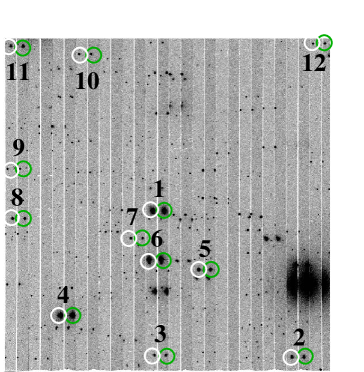
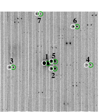
Figure 1: The polarimetric frames of the two fields for 1ES 1959+650 (top), and HB89 2201+044 (bottom), observed in the $R$ band. In both cases, the white and green circles indicate the locations of the blazar and field stars for the ordinary and extraordinary images, respectively, prior to the virtual masking. Labeled with 1 are the blazars, and with numbers larger than 1 the field stars whose fluxes were measured. The field of view is $9$ $\times$ $9$ arcmin, and East is up and North is to the right.

Multicolor polarimetry can provide information about the innermost part of an AGN. Thus, the wavelength dependence of polarization of blazars has been studied by several authors (see e.g., Brindle et al. 1986, and references therein). Among others, it can reveal the presence of more than one synchrotron component, and the dilution by thermal radiation from the parent galaxy (Maza et al. 1978). In consequence, we observed using $R$ and $B$ filters. Exposure times ranged between 60 and 120 seconds, strongly depending on the atmospheric conditions, the altitude of the blazars during the observations, and the chosen filter. We acquired sky flats and bias frames on regular basis. Atmospheric conditions were different throughout the observing time, from fairly good (no clouds, seeing full width at half maximum, FWHM $\sim$ 1 arcsec) to rather poor (cirrus, FWHM $\ga$ 2.5 arcsec). During poor observing conditions, we observed only in the $R$ band, where atmospheric extinction and scattering of spurious light by dust particles in the atmosphere are less dominant.

For the image pre-processing we used standard IRAF routines. We corrected all science frames by bias and flats in the usual way. However, for the data extraction and analysis we used IRAF tasks created by our group. Previous to the photometry, it was necessary to multiply the images by a virtual mask. This consists of an image with alternate stripes of $\sim 20$ arcsec width, with pixel values set to either one or zero. Our IRAF routines are tailored to appropriately handle zero-valued pixels within the aperture and the sky annulus. If there is one or more zero-valued pixels within the photometric aperture, the magnitude is not defined and the result from that aperture is discarded. Nonetheless, the final aperture size was well contained within the stripes, and magnitudes computed from apertures up to 10 arcseconds ($\sim$5 FWHM) were always defined. This procedure avoids contamination of the E images, in the aperture and sky annulus used for photometry by the O images, and vice-versa. Afterwards, we obtained the instrumental magnitudes and polarimetric data corresponding to the E and O images for the two blazars on each frame. The same procedure was carried out on stars evenly distributed on the field and suitably placed within the mask stripes (i.e. we rejected stars close to the edge of the stripes). We used them as estimators of the instrumental and foreground polarization, and to produce the differential light curves in both bands along the whole campaign.

To maximize the S/N ratio of our measurements, we carried out a careful selection of the aperture radius. We measured photometric and polarimetric quantities integrating blazar and stellar fluxes within 15 apertures, starting from 1 arcsec up to 10 arcsec. To select the final aperture we followed Howell (1989) and our own error analysis. While the former requires an aperture radius close to the FWHM of the sources, the latter requires the minimization of the error in the polarization degree and the polarization angle. Although the aperture that minimized these quantities slightly changed along the nights (just because the photometric conditions during the observations changed), the optimal aperture radius turned out to be always around 3 arcsec, which corresponds to the largest seeing value along the whole campaign. Since our goal is to analyze polarimetric variability and compare this along the observing nights, to carry out a photo-polarimetric analysis as homogeneous as possible we fixed the aperture radius to 3 arcsec in both data sets and throughout the campaign.

2.2 Stokes parameters

To obtain the normalized Stokes parameters we used four frames, each with a different position angle of the rotating plate (0, 22.5, 45, and 67.5 degrees). Their mathematical expressions are:

$$\begin{split}&Q=\frac{R_{\mathrm{Q}}-1}{R_{\mathrm{Q}}+1}\,,&U=\frac{R_{\mathrm{U}}-1}{R_{\mathrm{U}}+1}\,,\\ \end{split}$$ (1)

where

$$\begin{split}&R_{\mathrm{Q}}^{2}=\frac{I_{0}^{O}/I_{0}^{E}}{I_{45}^{O}/I_{45}^{E}}\,,&R_{\mathrm{U}}^{2}=\frac{I_{22.5}^{O}/I_{22.5}^{E}}{I_{67.5}^{O}/I_{67.5}^{E}}\,,\\ \end{split}$$ (2)

$I_{\beta}^{O}$ y $I_{\beta}^{E}$ are the object ordinary and extraordinary integrated fluxes, respectively, and $\beta$ is the position angle of the half-wave plate (Zapatero Osorio et al. 2005; Andruchow et al. 2011). Based on these parameters, we calculated the degree of polarization and corresponding position angle in the usual way:

$$\begin{split}&P=\sqrt{Q^{2}+U^{2}}\,,\\ &\Theta=\frac{1}{2}\mathrm{arctan}\left(\frac{U}{Q}\right)\,.\\ \end{split}$$ (3)

Error estimates for both parameters were computed using standard error propagation techniques. However, our final expressions were verified with and compared to the ones available in Patat & Romaniello (2006). This procedure was carried out equivalently for the two blazars, all the field stars labeled in Figure 1, and the polarized and unpolarized standard stars. To analyze the consistency of our error determination, we checked (and also always verified) that the magnitude of the individual polarimetric errors was comparable to the magnitude of the standard deviation of the polarimetric points within a given night.

2.3 Extrinsic polarization: Instrumental and foreground polarization

For the calibration and transformation of the data to the standard system (N-E-S-W, Lamy & Hutsemékers 1999), we observed highly polarized and unpolarized standard stars (Table 1) cataloged under Schmidt et al. (1992) and Turnshek et al. (1990). Following Patat & Romaniello (2006) and Patat & Taubenberger (2011), we analyzed the data obtained for the unpolarized standard stars to quantify the instrumental polarization per filter. We observed a standard unpolarized star every night, that was placed at exactly the same location than the blazars, coincidentally being the center of the CCD. CAFOS is known to have a dependency of the instrumental polarization with the position over the CCD, increasing towards the edges (see, e.g., Patat & Taubenberger 2011, for a careful characterization of the instrumental polarization of CAFOS). Thus, our observing strategy was diagramed to properly characterize the instrumental polarization at the position of the target. A characterization of the instrumental polarization of CAFOS is beyond the scope of this work. From these observations we calculated the Stokes parameters in the usual way per night and per filter, and we averaged them along the whole campaign. In agreement with previously reported values, we found a low contribution of the instrumental polarization at the center of the CCD. For the $R$ band we found Q_instr = 0.029% and U_instr = -0.015%, and for the $B$ band we found Q_instr = -0.14% and U_instr = -0.013%. As a complementary checkup of the expected polarization behavior of CAFOS, we computed the polarization degree of all the field stars. Assuming that these are unpolarized, we see a clear dependency of their polarization degree with their distance to the center of the CCD.

We also estimated a lower limit to the foreground polarization using the stars $5$, $6$ and $7$ in the case of 1ES 1959+650, and stars $2$ and $5$ in the case of HB89 2201+044. Labels are as in Figure 1. Foreground polarization is small: $0.7\%$ in $R$ and $0.9\%$ in $B$ for 1ES 1959+650 and and $0.3\%$ in $R$ and $0.4\%$ in $B$ for HB89 2201+044. This is consistent with the upper limits estimated using $P_{\mathrm{max}}\leq 9E_{\mathrm{B-V}}$ (Hough 1996; Serkowski et al. 1975), with the $E_{\mathrm{B-V}}$ indexes obtained from the NASA/IPAC Extragalactic Database (Schlafly & Finkbeiner 2011), giving $P_{\mathrm{V}}<1.4\%$ for 1ES 1959+650 and $P_{\mathrm{V}}<0.34\%$ for HB89 2201+044. Thus, from now on all the polarimetric quantities are corrected by instrumental and foreground polarization in the following fashion:

$$\begin{split}&Q_{\mathrm{corr}}=Q_{\mathrm{obs}}-Q_{\mathrm{instrumental}}-Q_{\mathrm{foreground}}\,,\\ &U_{\mathrm{corr}}=U_{\mathrm{obs}}-U_{\mathrm{instrumental}}-U_{\mathrm{foreground}}\,.\\ \end{split}$$ (4)

In all cases, position angles were transformed to the Standard system using data from highly polarized standard stars.

Finally, we estimated the unbiased degree of polarization, $P_{0}$. We use the expression,

$$P_{0}=\sqrt{P^{2}-a*P_{\mathrm{err}}^{2}}\leavevmode\nobreak\ ,$$ (5)

as specified in Simmons & Stewart (1985). $P_{0}$ was computed using the maximum likelihood estimator that can be found in their work ($a=1$). For both blazars, the correction is one order of magnitude smaller than the polarimetric errors. Thus, we did not apply the correction since it is statistically negligible. In the case of HB89 2201+044, we did not calculate this correction in the B-band because there are not enough data points.

3 Photometric and polarimetric analysis

3.1 Photometry

The differential light curves for the $B$ and $R$ filters for both blazars, spanning the whole observational campaign, are shown in Figure 2 (see Andruchow et al. 2011, for details about the construction of the light curves). Particularly, to construct the differential and control light curves of 1ES 1959+650, we used the stars labeled 2 and 8, respectively (see Figure 1) for both $R$ and $B$ bands. For HB89 2201+044, the comparison star is number 3, while the control star is number 4. This applies to both bands.

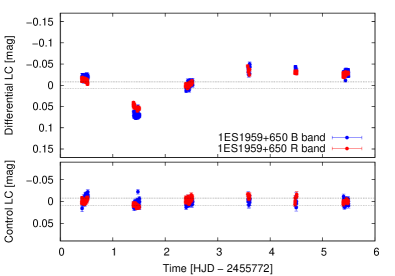
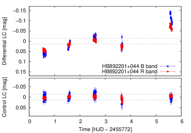
Figure 2: Differential (top sub-panels) and control (bottom small sub-panels) light curves (LC) in magnitudes as a function of the Heliocentric Julian Date (HJD) for the two blazars observed in this work. Left: 1ES 1959+650, $B$ and $R$ bands. Right: HB89 2201+044, $B$ and $R$ bands. Horizontal black-dashed lines show two times the $B$ standard deviation of the control light curves. Red data points correspond to $R$ band data, while blue data points to the $B$.

To characterize the variability in our photo-polarimetric data we used the scaled $C$ criterion (Howell et al. 1988), one of the most reliable tools for this kind of analysis (Zibecchi et al. 2017). The criterion is defined as the quotient between the standard deviation of the differential light curve of the blazar (DLC), $\sigma_{\mathrm{DLC}}$, and the standard deviation of the control light curve (CLC), $\sigma_{\mathrm{CLC}}$, scaled by a factor $\Gamma$ that takes into consideration the different relative brightnesses between the AGN and the comparison and control stars. This is represented as the scaled confidence parameter, $\mathrm{C}_{\Gamma}$. When $\mathrm{C}_{\Gamma}\geq 2.576$, variability is detected at least with a 99.5% confidence level.

The standard deviations of the final control light curves are $\sigma$ = 7.9 milli-magnitudes (mmag) in the $B$ band and $\sigma$ = 6.9 mmag in the $R$ band for 1ES 1959+650, and $\sigma$ = 13.6 mmag in $B$ and $\sigma$ = 6.0 mmag in $R$ for HB89 2201+044.

The behavior of the $B$ and $R$ bands is similar. In consequence, Table 2 shows the results for 1ES 1959+650 and HB89 2201+044 for the $R$ band alone. In both bands, neither of the two blazars presented intra-night variability. However, in the case of 1ES 1959+650 there is evidence of variability on longer time scales, manifested as a sustained decrease and increase of flux ($\Delta R,B\approx 0.1$ mag) that took place during the first 3 nights. For HB89 2201+044, during the last 2 nights we detected an increase of flux ($\Delta R,B\approx 0.15$ mag). In the case of 1ES 1959+650, when only one individual night is evaluated no variability is observed, while analyzing the whole campaign returns $\mathrm{C}_{\Gamma}=2.01$. The corresponding value for HB89 2201+044 is $\mathrm{C}_{\Gamma}=9.580$. Thus, both blazars show inter-night variability, although for 1ES 1959+650 it might be marginal. In the particular case of HB89 2201+044, contrary to 1ES 1959+650 we detected intra-night variability in two of the six nights. At this stage it was unclear to us if this observed variability was produced by physical processes occurring in the source, or were the result of fluctuations in the seeing during the observing nights. This point is addressed later.

Table 2: Variability parameters for the $R$ light curves on different nights for 1ES 1959+650 (top) and HB89 2201+044 (bottom). From left to right we provide date (Col. 1), target-comparison light curve dispersion (Col. 2), control-comparison light curve dispersion (Col. 3), scaled confidence parameter (Col. 4), variability classification following adopted criterion (Col. 5) and number of $R$ band data points (Col. 6). MARG. corresponds to marginal detection of variability.

Date	$\sigma_{\mathrm{DLC}}$	$\sigma_{\mathrm{CLC}}$	$\mathrm{C}_{\Gamma}$	Variable?	N
(mm/dd/yyyy)	($R$)	($R$)
1ES 1959+650
07/29/2011	0.004	0.004	0.986	NO	33
07/30/2011	0.004	0.003	1.263	NO	32
07/31/2011	0.004	0.005	0.831	NO	36
08/01/2011	0.007	0.017	0.436	NO	12
08/02/2011	0.005	0.033	0.164	NO	12
08/03/2011	0.003	0.002	1.514	NO	28
WC	0.031	0.016	2.010	MARG.	153
HB89 2201+044
07/29/2011	0.005	0.005	1.170	NO	27
07/30/2011	0.006	0.002	2.951	YES(?)	32
07/31/2011	0.005	0.005	2.035	NO	36
08/01/2011	0.007	0.007	1.203	NO	20
08/03/2011	0.009	0.003	4.478	YES(?)	32
WC	0.039	0.005	9.580	YES	147

3.2 Polarimetry

To characterize the polarization state of the blazars, as specified in Sect. 2 we calculated their linear polarization, $P$, and position angle, $\Theta$. The effect of the galaxy is more evident in $P$ (Andruchow et al. 2008; Cellone et al. 2007). In consequence, along this work we will specify quantities in ($P$,$\Theta$) rather than in ($Q$,$U$). Due to poor observing conditions we only have polarimetric data along the whole campaign in the $R$ band for 1ES 1959+650. In the case of HB89 2201+044, on the fifth night we lack polarimetric data. Their mean values and standard deviations are summarized in Table 3, and their temporal evolution can be seen in Figure 3.

Table 3: Mean values for the polarization degree, $P$, and polarization angle, $\Theta$, for the blazars 1ES 1959+650 and HB89 2201+044.

Blazar	$\langle P\rangle$	$\langle\Theta\rangle$	Band
1ES 1959+650	6.97 $\pm$ 0.50	145.40 $\pm$ 4.66	$B$
1ES 1959+650	6.17 $\pm$ 0.41	144.33$\pm$ 4.75	$R$
HB89 2201+044	0.70 $\pm$ 0.46	168.52 $\pm$ 32.28	$B$
HB89 2201+044	0.38 $\pm$ 0.30	188.44 $\pm$ 37.45	$R$

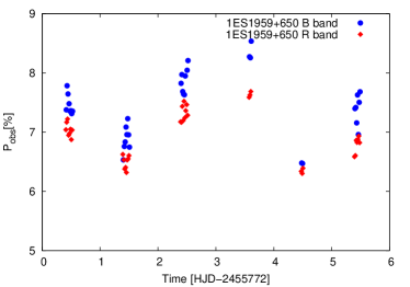
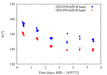
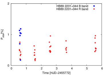
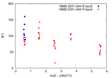
Figure 3: Time evolution of the polarimetric parameters for the $B$ (blue circles) and $R$ (red diamonds) bands, corrected by instrumental and foreground polarization. Top: the polarization degree in percentage, $P$ [%] (left) and the polarization angle in degrees, $\Theta$ [$\circ$] (right) for 1ES 1959+650. Bottom: equivalently, but for HB89 2201+044.

We analyzed the behavior of $P$ and $\Theta$ throughout the whole campaign. For 1ES 1959+650, $P$ is relatively high ($\sim 7\%$, see, e.g. Andruchow et al. 2005, for comparable results). A visual inspection of the polarimetric data along the campaign shows some inter-night variability, while the angle presents a slight rotation. On the contrary, HB89 2201+044 seems to be steady and shows an erratic behavior for the polarization angle with large error bars, which can be attributed to the fact that this parameter is not well defined because of the low polarization.

To estimate if both blazars show inter and intra-night polarimetric variability, we carried out a statistical analysis fully described in Kesteven et al. (1976). In this case, a given source is qualified as variable if the probability of exceeding their $\chi^{2}$ value is smaller than $0.1\%$, and not variable if the probability is larger than $0.5\%$. Due to the scarcity of polarimetric data for the $B$ band in HB89 2201+044, we carried out this analysis exclusively in the $R$ band. The analysis of intra-night variability retrieved probability values between $18\%$ and $86\%$ for 1ES 1959+650, and between $30\%$ and $76\%$ for HB89 2201+044, clearly favoring the absence of intra-night variability. When the whole campaign is analyzed, probability values of 10^-8% and 10^-45% are obtained for both blazars, favouring the presence of inter-night variability.

3.2.1 Impact on $P$ of the aperture choice

While analyzing the depolarizing effect that is introduced by the host galaxy on the AGN, careful considerations have to be taken into account regarding seeing and aperture. Seeing affects in a different way the AGN (point source) and the galaxy (extended source). Consequently, a variation in seeing introduces (or removes) a percentage of unpolarized light within the aperture from the galaxy which in general will be different to the introduced (or removed) percentage of light from the nucleus (see Andruchow et al. 2008, for the impact of seeing in this type of measurements). Therefore, to quantify how much the host galaxy affects our derived values of the polarization state of both blazars, we analyzed only the night that showed almost negligible seeing variability (August 3^rd, 2011). In this way, the variability to be measured is most likely due to the intrinsic changes in the polarization state of the blazars and not due to changes caused by our Earth’s atmosphere. As it is expected, we observed a decrease of the degree of polarization when larger apertures are being used, revealing the impact of the host galaxies in our measured values. This effect can be appreciated in Figure 4 in the case of 1ES 1959+650 for the $R$ band, and its detection is independent of the choice of filter or blazar. Altogether, these results show that one has to choose a reliable criterion before fixing the aperture to extract fluxes from photo-polarimetric data. Our particular choice has been already specified in Sect. 2.1. It is worth to mention that $\Theta$ is not affected by changes in the photometric aperture.

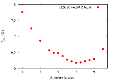
Figure 4: Behavior of the polarization degree with the aperture for the blazar 1ES 1959+650 in the $R$ band.

4 Results

As previously mentioned, two (related) effects should be considered when dealing with polarimetric time series of AGN with prominent host galaxies: the host starlight introduces a depolarazing effect, and its amount will be variable if seeing changes along the observations. Moreover, both the depolarization and its variations due to seeing will depend on wavelength. Similar effects apply to photometric light-curves, where the host starlight dilutes any intrinsic AGN variability, and introduces spurious variability under seeing fluctuations. In this Sect. we will carefully analyze these effects.

4.1 Determination of observed structural quantities

To recover the intrinsic polarization of the AGNs we determined the structural parameters of both blazar host galaxies. To this end we combined the images per blazar and per filter that were taken without the polarizer (2 images in $B$ band and 2 images in $R$ band for 1ES 1959+650, and 6 images in $B$ and 2 images in $R$ for HB89 2201+044). These images were taken during the night that presented not only the lowest seeing but also the lowest seeing variability (August 3^rd, 2011). In the particular case of HB89 2201+044, eastwards from the blazar a bright star can be observed. We considered this, and the effect that this introduces over the determination of the intrinsic parameters of the host galaxy, as addressed in the next Sect.

To determine the structural parameters of the host galaxies we used the combined power of IRAF’s tasks ellipse and nfit1d. Before carrying out the isophotal fit we removed the field stars and the neighboring galaxies with a mask. During this process we chose appropriate functions that best match the combined surface brightness profile of the host galaxy, and the surface brightness profile of the AGN, combined with the changes in brightness induced by our Earth’s atmosphere.

For the AGN we considered a Gaussian function with the following parameters:

$$g(a_{\mathrm{AGN}})=g_{\mathrm{0}}\times\mathrm{e}^{-(a_{\mathrm{AGN}}/2\sigma)^{2}},$$ (6)

where $a_{\mathrm{AGN}}$ corresponds to the semi-major axis of the AGN, FWHM = 2$\sqrt{2\,\ln(2)}\leavevmode\nobreak\ \sigma$ accounts for the seeing (FWHM), and $g_{\mathrm{0}}$ corresponds to the amplitude of the Gaussian. In this case, for 1ES 1959+650 we considered FWHM = 1.87 pixels and FWHM = 2.53 pixels for the $R$ and $B$ bands, respectively, and for HB89 2201+044 the derived values were FWHM = 2.18 pixels and FWHM = 2.72 pixels, in the same order. All values were determined averaging the FWHM of several stars inside the field of view, selected because they showed no saturation and were located close to the blazars (see all stars labeled in Figure 1).

To represent the surface brightness profile of the host galaxy we used Sersic’s law:

$$I(a_{\mathrm{HG}})=I_{\mathrm{o}}\times\mathrm{e}^{-(a_{\mathrm{HG}}/r_{\mathrm{0}})^{1/n}},$$ (7)

where $I_{\mathrm{o}}$ is the central surface brightness, $r_{\mathrm{0}}$ is a pseudo scale parameter, and $n$ ($n>0$) corresponds to the Sersic’s index, a parameter that determines the shape of the brightness profile. All parameters were fitted to the data. Once the best fit parameters were obtained, we determined the structure, the flux, and the instrumental magnitude of the host galaxy. All fit parameters are summarized in the upper part of Table 4.

4.2 Recovery of the intrinsic parameters of the host galaxies

To characterize the effect of the FWHM on the previously determined structural parameters, instead of following the approach described in Trujillo et al. (2001), we build up an empirical relationship, with the goal of recovering the intrinsic parameters of the host galaxy when the observed ones are used as input. Although the latter is not a direct method, we opted for this more conservative treatment. The sampling of our data is not optimal for 2-D fitting algorithms such as GALFIT (Peng et al. 2002) to give reliable results. This was concluded after several trials on simulated images with similar characteristics as our observations. We finally opted for an approach which uses synthetic data, allowing us to better understand the behavior and correlations between parameters when seeing changes, thus identifying regions of parameter space where the recovery of intrinsic parameters might not be reliable. To this end we generated simulated host galaxies using Sersic’s law (Eq. 7) changing the values for $a_{HG}$ and $n$, and arbitrarily fixing $I_{\mathrm{o}}$. These images were then convolved with a Gaussian function with different values of FWHM to account for different values of seeing. We obtained 1890 images, that we re-analyzed to recover their structural parameters in the exact same fashion as discussed in Sect. 4.1. Analyzing the parameters obtained by the fitting algorithms, and comparing them to the ones used to generate the synthetic data, we found that they are not directly related in a one-by-one fashion, but following some relations that involve other structural parameters. For example, we found that the fitted effective radius depends on the effective radius used to create the synthetic image, but also on the Sersic’s index. This is nothing more than the reflection of a strong coupling between parameters. Using these as empirical relations we input our previously determined structural parameters, and obtained the intrinsic (i.e., seeing free) parameters. The lower panel of Table 4 summarizes our results. After a quick comparison between the top (observed) and bottom (recovered) parameters of the two host galaxies we see, for instance, that the observed Sersic’s index is systematically smaller than the recovered one. A lower $n$ would imply a less steep brightness profile, which is exactly the impact that seeing has over point sources (Trujillo et al. 2001).

Table 4: Parameters of model fits for both blazars in the $R$ and $B$ bands. Top: parameters derived from the observations. Bottom: recovered intrinsic parameters of the host galaxies once seeing has been accounted for.

Band	$a_{\mathrm{HG}}$	$n$	I0	mgal
	(pix)		(ADU/pix2)	(mag)
1ES 1959+650, observed
$B$	14.3564	1.9523	486.31	16.295
$R$	12.5675	1.7838	1941.50	14.033
HB89 2201+044, observed
$B$	14.3568	2.1363	1234.52	15.391
$R$	18.7721	2.1779	7471.17	12.875
1ES 1959+650, recovered
$B$	14.5169	1.9734	476.85	16.332
$R$	12.5264	1.8156	1872.09	14.140
HB89 2201+044, recovered
$B$	14.5017	2.1615	1221.48	15.429
$R$	20.0153	2.2351	8373.34	12.723

4.3 Correction of the polarimetric measurements by the contribution of the host galaxy

To correct for the depolarizing effect that the host galaxy introduces in our measurements, we have to take into account the following relation:

$$P=P_{\mathrm{obs}}\left(1-\frac{F_{\mathrm{G}}}{F_{\mathrm{AGN}}+F_{\mathrm{G}}}\right)^{-1}\;,$$ (8)

where $F_{AGN}+F_{G}$ is the observed standard flux of the AGN plus host galaxy, and $F_{G}$ is the standard flux of the host galaxy, both wavelength dependent and at this point unknown (see Andruchow et al. 2008, for a full description on the formulas of Eq. 8). To estimate $F_{G}$ we made use, one more time, of synthetic data. We simulated a host galaxy per band, using as input parameters the intrinsic parameters listed in the bottom panel of Table 4, and integrated the flux inside the aperture that was originally considered to extract the fluxes of real data (see Sect. 2 for further details). However, before this we convolved this synthetic image with a Gaussian kernel, whose standard deviation reflected the seeing of the true data, not globally but image by image. In particular, this seeing was estimated averaging the seeing values of unsaturated stars in the field of view. As an example, if during a given night we collected four images, each one with one of the four position angles of the rotating plate, we calculated the average seeing of each image and used it to convolve the image of the host galaxy. We end up with four synthetic images, that were integrated to determine the expected standard flux of the host galaxy affected by the time-dependent seeing. However, we still need to overcome the fact that $F_{AGN}+F_{G}$ is still unknown. To estimate this we can assume the following relation:

$$\frac{f_{*}}{F_{*}}=\frac{f_{\mathrm{AGN}}+f_{\mathrm{G}}}{F_{\mathrm{AGN}}+F_{\mathrm{G}}}\;,$$ (9)

where, neglecting color-dependent terms, the relation shows that the flux ratio between instrumental and standard fluxes of a given reference star, $\frac{f_{*}}{F_{*}}$, should equal the flux ratio between the instrumental and standard fluxes of the blazar plus host galaxy, $\frac{f_{\mathrm{AGN}}+f_{G}}{F_{\mathrm{AGN}}+F_{G}}$.

To calculate the standard magnitudes (and thus fluxes, $F_{*}$) of the reference stars, we used data of photometric standard stars of two Landolt fields, SA $115$ and SA $114$ (Landolt 1992), that we acquired during a photometric night and without polarizer. For the stars in the field of 1ES 1959+650, our results agree with those by Pace et al. (2013). We found no previously published standard magnitudes for stars in the field of HB89 2201+044, so we report them in Appendix A.

With $F_{*}$ computed we obtained, image by image, $F_{AGN}+F_{G}$. Using this quantity in Eq. 8 we calculated four correction terms per polarimetric point (again, each one corresponding to each rotation angle, and each one with its respective seeing value) and calculated a last correction term by averaging these four. Finally, we re-computed the polarization degree along the whole campaign taking into account this correction. The results of polarization degree for the whole campaign, for the $R$ band and the blazar 1ES 1959+650, can be seen in Figure 5. In this case, the averaged difference between both polarization states is of the order of 1% (see Table 5 for a complete picture of both blazars and both bands).

Furthermore, as described in Sect. 3.2, we re-calculated the probability values associated to intra and inter-night variability, but now using the polarimetric points corrected by the depolarizing effect introduced by the host galaxies. Although results do not change (we found again no intra-night variability but inter-night variability) the probability values significantly decrease, around a factor of 3, which would point out the need of correcting for the effect described in this Sect.

Table 5: Mean values for the polarization degree with ($P$) and without ($P_{\mathrm{intrinsic}}$) the contribution of the host galaxy for the blazars 1ES 1959+650 and HB89 2201+044.

Blazar	$\langle P\rangle$	$\langle P_{\mathrm{intrinsic}}\rangle$	Band
1ES 1959+650	6.97 $\pm$ 0.50	7.64 $\pm$ 0.64	$B$
1ES 1959+650	6.17 $\pm$ 0.41	7.06 $\pm$ 0.49	$R$
HB89 2201+044	0.70 $\pm$ 0.46	1.01 $\pm$ 0.67	$B$
HB89 2201+044	0.38 $\pm$ 0.30	0.62 $\pm$ 0.49	$R$

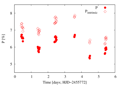
Figure 5: Polarimetric behavior of the blazar 1ES 1959+650 along the whole campaign in the $R$ band, corrected only by instrumental polarization (P, red filled circles) and instrumental polarization plus the contribution of the host galaxy (P_intrinsic, red empty diamonds).

4.4 Impact of seeing on our polarimetric measurements

As previously mentioned, the changes in the photometric quality during the observing nights may introduce spurious variability that has to be considered when microvariability is being reviewed. Seeing strongly degrades measurements. Furthermore, as a result of seeing variability a given fixed aperture introduces a larger or lower amount of unpolarized light coming from the host galaxy. As a result, the depolarizing effect changes with seeing, affecting the measurements of polarized light of the nucleus, if not corrected. Seeing variability directly reflects into the flux ratio between the nucleus and the galaxy, because both components have a different brightness distribution and are, in consequence, differently affected. Our seeing values range between 1 and 3 arcsec, as seen on the horizontal axis of Figure 6. As mentioned in previous sections, our chosen aperture was set to be 3 arcsec and was considered fixed along the whole campaign. Therefore, the chosen aperture is larger than the seeing values along the campaign and always contains, as consequence, most of the flux of the nucleus (Howell 1989). To test the impact of seeing in our polarimetric measurements, and the importance of correcting for the depolarizing effect of the host galaxy, we did the following exercise. First, we re-calculated all our polarimetric (and thus photometric) quantities using an aperture of 2 arcsec. Our results for the $R$ band and the blazar 1ES 1959+650 can be seen in the left part of Figure 6. While the red filled circles show the polarimetric measurements for an aperture equal to 3 arcsec, the pink filled squares show polarimetric values for an aperture of 2 arcsec. Neither of them have been corrected for the depolarizing effect introduced by the host galaxy. As the Figure clearly shows, the polarization is larger for the smaller aperture. This is simply because a smaller aperture implies a smaller contribution of the host galaxy depolarizing effect which, in turn, translates into a larger polarization. Then, we corrected for the depolarizing contribution of the host galaxy for both apertures, as explained in previous Sections. Our results can be seen in the right panel of Figure 6, following the same color and point-code. Not surprisingly, the polarization level of both apertures is on average the same (and higher than uncorrected values), showing again the relevance of correcting for the host galaxy.

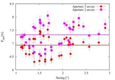
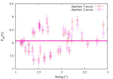
Figure 6: Behavior of the polarization degree with seeing for 1ES 1959+650 in the $R$ band when two fixed apertures are considered. In the left panel data points correspond to the observed polarization, $P_{\mathrm{obs}}$, while the right panel shows the polarization corrected by the contribution of the host galaxy, $P_{\mathrm{intrinsic}}$. Horizontal lines following the same color-code indicate mean values of polarization and are plotted to guide the readers eye.

4.5 Corrected photometry along the campaign

Figure 7 shows the photometric behavior of the two blazars along the whole campaign, when the contribution of the host galaxy has been removed. For a better visualization, both $B$ band quantities were shifted by one magnitude. We observed photometric variability in both blazars along the campaign, and a similar trend in inter-night variability for the case of 1ES 1959+650. We observed no significant intra-night variability. In particular, for 1ES 1959+650, our results are similar to the values found by Sorcia et al. (2013), where the source showed a minimum and maximum of brightness of $R=15.2$ mag and $R=14.08$ mag, respectively.

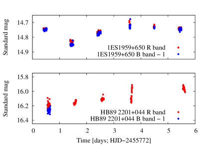
Figure 7: Standard magnitudes of the blazar without the contribution of the host galaxy for 1ES 1959+650 (top) and HB89 2201+044 (bottom) for both filters ($R$-band in red, $B$-band in blue). $B$-band values were shifted in 1 magnitude for a better visualization.

5 Discussion and conclusions

Blazars are known to have extreme photo-polarimetric variability. Some examples of these are AO 0235+164 (Cellone et al. 2007), or PKS 1510-089 (Aleksić et al. 2014). The last object reached a peak flux of $18$ mJy in the $R$ band while the quiescent level flux is typically $\sim 2$ mJy. During this major optical flare, the optical polarization degree increased to $>30\%$. This reveals the importance of photo-polarimetric follow-ups of blazars, with the main goal to understand and properly model the source of their variability. In this work we have undertaken a photo-polarimetric follow-up that included two targets, an HBL object (1ES 1959+650) and an LBL object (HB89 2201+044). During our observations, we simultaneously registered their polarimetric and photometric behavior. We analyzed the behavior of their linear polarization computing the parameters $P$ and $\Theta$ throughout the whole campaign. 1ES 1959+650 seems to present a very moderate inter-night variability, while the angle has a slight ($\sim 10$ deg.) rotation along the campaign. As we mentioned in Sect. 2, the HBLs should show statistically lesser amounts of polarized light than that of LBLs. This behavior is not in agreement with our results, since we found a $P\sim 7\%$ for 1ES 1959+650, while HB89 2201+044 shows a polarization consistent with zero when errors at two-sigma level are considered ($P\sim 0.70\%$). Regarding HB89 2201+044, one explanation could be that the object is currently in a low activity state. There are not enough data nor literature available to say the contrary. Further simultaneous photometric and polarimetric observations of this object are required. Carrying out a statistical analysis, we find a non-detection of intra-night polarimetric microvariability in both blazars, while a significant polarimetric variability is evident when the whole campaign is taken into consideration. We also observe a very moderate inter-night photometric variability for HB89 2201+044 in filter $B$, and in both filters for 1ES 1959+650.

Our targets are relatively nearby objects. Their host galaxies introduce a depolarizing effect which, in turn, can lead to systematic errors in the derived photo-polarimetric quantities when seeing conditions vary with time. We have modeled the incidence of the host galaxy and, for the first time, we have corrected our polarimetric data by the depolarizing effect introduced by the host galaxy in an auto-consistent way, this is, using our own data to obtain its structural parameters. Simultaneously, we have considered spurious variability introduced by varying seeing conditions into our microvariability analysis. Comparing our values with and without correcting for the host galaxies, the intrinsic polarization is $1\%$ and $0.3\%$ higher for 1ES 1959+650 and HB89 2201+044, respectively, while the behavior of intrinsic polarization with time is the same than the observed polarization in both blazars. For the case of 1ES 1959+650, if we compute the ratio of polarizations in $B$ and $R$ bands, not taking into consideration the host galaxy, gives $P_{\mathrm{B}}/P_{\mathrm{R}}=1.12\pm 0.02$. This value can be explained as follows: blazars are in elliptical galaxies which present dominant starlight emission in $R$ band. In consequence, the depolarizing effect introduced by the host galaxy is smaller in the $B$ band than in the $R$ band. Therefore, the observed polarization in $B$ is expected to be larger than in $R$. After applying the host galaxy correction, we obtained $P_{\mathrm{B}}/P_{\mathrm{R}}=1.08\pm 0.02$, which indicates that the polarization is almost the same in both band. The difference between both ratios is significant at a $\sim 1.5\,\sigma$ level. Larger differences could be obtained under different atmospheric conditions and for blazars with other host-galaxy to AGN flux properties. Therefore, if we do not take into account the effect introduced by the host galaxy there would be a tendency to retrieve erroneous results. This could be relevant in studies of frequency dependent polarization (see e.g., Barres de Almeida et al. 2010). Finally, the presence of dust features in host galaxies, such as the case of 1ES 1959+650 (Heidt et al. 1999), may be another source of uncertain. Their effects depend on wavelength, so they could affect polarization measurements in a different amount in each photometric band. However, we believe the quality of our data is not sufficient to recognize this effect from our polarimetric uncertainties.

In general, our work shows that if the host galaxy is not properly taken into account, and also if changing seeing conditions are not take care of, a significant error in the computation of the polarization degree of blazars can be produced. This, in turn, could end up in misleading models or conclusions derived from erroneous polarization states. And the spurious results are intensified if we study high polarized objects, such as the HBL type.

Appendix A Standard magnitudes

Standard magnitudes and associated 1$\sigma$ errors of the field stars of HB89 2201+044 can be found in Table 6. These standard magnitudes were obtained following the procedure described in Sect. 4. The labels of Table 6 correspond to those of Figure 8. For stars in the field of 1ES 1959+650, the standard magnitudes and their errors are in agreement with Pace et al. (2013).

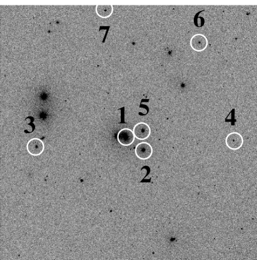
Figure 8: The field of view without polarizer ($9$ $\times$ $9$ arcmin) of HB89 2201+044. The white circles indicate the locations of the blazar (1) and field stars ($>$1). East is up and North is to the right.

Table 6: Standard magnitudes of the field stars of HB89 2201+044 in $R$ and $B$ bands.

Star	$R$	$B$
2	13.427$\pm$0.004	14.190$\pm$0.002
3	14.423$\pm$0.007	15.549$\pm$0.004
4	15.527$\pm$0.022	17.671$\pm$0.011
5	13.116$\pm$0.004	14.678$\pm$0.002
6	14.159$\pm$0.014	16.793$\pm$0.007
7	15.718$\pm$0.020	17.337$\pm$0.010