1 Introduction

The mathematical modelling of electric circuits often yields time-dependent systems of nonlinear differential algebraic equations (DAEs), see [13, 16, 19]. In radio frequency applications, high-frequency oscillations appear, whose amplitude and/or frequency change slowly in time. Hence a transient simulation of initial value problems of the DAEs is inefficient, because a numerical integrator has to capture each oscillation.

A multidimensional signal representation yields an alternative approach. Brachtendorf et al. [5] derived an efficient model consisting of multirate partial differential algebraic equations (MPDAEs). Analysis and simulation of the MPDAE model in the case of amplitude modulation without frequency modulation is given in [1, 6, 25, 26, 35].

In the case of frequency modulation, Narayan and Roychowdhury [24] formulated a system of (warped) MPDAEs, where a local frequency function represents a degree of freedom. Hence an additional condition is required to determine a solution, which allows for an efficient numerical simulation. On the one hand, the MPDAEs together with phase conditions or similar constraints were considered in [27, 28, 30, 33, 36]. On the other hand, the identification of optimal solutions, which exhibit a minimum amount of oscillations in some sense, implies necessary conditions. MPDAEs with optimal multidimensional representations were investigated in [2, 3, 11, 17, 18, 20, 31, 32]. A survey on all the above cases can be found in [29].

In this paper, we consider initial-boundary value problems of (warped) MPDAEs in the case of frequency modulation. A method of lines yields a system of DAEs, whose numerical solution approximates the exact solution. The local frequency function is included in this approximative system. The analytical as well as numerical properties of a DAE system are characterised by its index, where different concepts exist, see [12, 15, 21]. We analyse the differential index of the system from the method of lines. Therein, we assume that the circuit model consists of semi-explicit DAEs of index one. The focus is on the method of lines including a necessary condition for an optimal solution from [20, 31]. In addition, the application of a phase condition going back to [24] is analysed. On the one hand, we perform a structural analysis of the DAE systems. On the other hand, we identify the index under certain assumptions. It follows that the index increases in most of the cases depending on the inclusion of differential variables or algebraic variables in the additional condition. Furthermore, we discuss the determination of the index by a numerical method, see [10], to confirm our analysis.

The paper is organised as follows. We review the multidimensional signal model, the MPDAE system and the method of lines in Section 2. We analyse the structure of the resulting systems of DAEs and determine their index in Section 3 and Section 4, respectively. Finally, Section 5 depicts results from numerical simulations of a ring oscillator.

2 Multirate Model

We review the modelling and simulation by MPDAEs.

2.1 Problem definition

Let the mathematical model of an electric circuit be a system of DAEs in the general form

$$\frac{\mbox{d}{q}({x}(t))}{\mbox{d}t}={f}({b}(t),{x}(t)).$$ (1)

The solution ${x}:\mathbbm{R}\rightarrow\mathbbm{R}^{n}$ includes unknown voltages and currents. The function ${b}:\mathbbm{R}\rightarrow\mathbbm{R}^{n_{\rm in}}$ introduces predetermined input signals. The nonlinear functions ${q}:\mathbbm{R}^{n}\rightarrow\mathbbm{R}^{n}$ and ${f}:\mathbbm{R}^{n_{\rm in}}\times\mathbbm{R}^{n}\rightarrow\mathbbm{R}^{n}$ depend on the solution. Let ${x},{q},{f}$ be sufficiently smooth and ${b}$ be continuous. Without loss of generality, we choose the initial time $t_{0}=0$. An initial value problem is given by

$${x}(0)={x}_{0}$$ (2)

with consistent initial values ${x}_{0}\in\mathbbm{R}^{n}$.

In radio frequency applications, the solution or some of its components represent high-frequency oscillations. We assume that the input signals change slowly in a total time interval $[0,t_{\rm end}]$. The input signals control the amplitude and/or frequency of the solution. Thus the function ${x}$ exhibits a huge number of oscillations in the total time interval. Concerning an initial value problem (1), (2), a numerical integration method has to capture each oscillation by several time steps. Hence a transient simulation becomes inefficient due to a huge computational effort.

2.2 Multirate partial differential algebraic equations

A multivariate signal model is able to decouple the slow time scale and the fast time scale in the problem. The solution ${x}$ of (1) is represented by a multivariate function ${\hat{x}}:[0,t_{\rm end}]\times[0,1]\rightarrow\mathbbm{R}^{n}$. The second time scale is standardised to the unit interval $[0,1]$. The input signals ${b}$ do not require a multivariate modelling, because they are assumed to be slowly varying functions. The system of DAEs (1) changes into the MPDAEs, see [24, Eq.(16)],

$$\frac{\partial{q}({\hat{x}}(t_{1},t_{2}))}{\partial t_{1}}+\nu(t_{1})\frac{\partial{q}({\hat{x}}(t_{1},t_{2}))}{\partial t_{2}}={f}({b}(t_{1}),{\hat{x}}(t_{1},t_{2})).$$ (3)

Therein, the local frequency function $\nu:[0,t_{\rm end}]\rightarrow\mathbbm{R}$ represents a degree of freedom in the multivariate modelling. We assume that ${\hat{x}}$ is smooth and $\nu$ is continuous. The system (3) is also called ’warped MPDAEs’ due to the introduction of the local frequency function, which deforms the second time scale. The equations (3) reveal a hyperbolic structure with a specific form of characteristic curves, see [27, Sect.4].

Either initial-boundary value problems or biperiodic boundary value problems are considered for the system of MPDAEs (3). In this paper, we examine initial-boundary value problems, i.e.,

$${\hat{x}}(0,t_{2})={\hat{x}}_{0}(t_{2}),\quad{\hat{x}}(t_{1},t_{2}+1)={\hat{x}}(t_{1},t_{2})\quad\mbox{for all}\;\;t_{1}\geq 0\;\;\mbox{and}\;\;t_{2}\in\mathbbm{R}$$ (4)

with a predetermined periodic function ${\hat{x}}_{0}:[0,1]\rightarrow\mathbbm{R}^{n}$. The initial condition has to contain the initial values (2) by ${\hat{x}}_{0}(0)={x}_{0}$. If the solution of the initial-boundary value problem has a relatively simple form with a low amount of oscillations in the domain of definition $[0,t_{\rm end}]\times[0,1]$, then a numerical solution can be done efficiently. The reason is that a coarse grid captures the multivariate function sufficiently accurate.

A solution of the initial-boundary value problem (3), (4) implies a solution of the original initial value problem (1), (2) by

$${x}(t):={\hat{x}}\left(t,\Psi(t)\right)\qquad\mbox{with}\qquad\Psi(t):=\int_{0}^{t}\nu(\tau)\;\mbox{d}\tau,$$ (5)

see [24, p. 902]. More details on the modelling by (warped) MPDAEs can be found in [29, 33].

2.3 Optimal solutions

In the system of MPDAEs (3), the local frequency function represents a degree of freedom. The aim is to obtain a solution ${\hat{x}}$ with a low amount of oscillations. Real-valued weights $w_{1},\ldots,w_{n}\geq 0$ are considered for an optimisation in each component. At least one weight must be positive. Let ${W}:={\rm diag}(w_{1},\ldots,w_{n})\in\mathbbm{R}^{n\times n}$. In [20], the minimisation of the functional

$$J({\hat{x}})=\int_{0}^{T_{1}}\int_{0}^{T_{2}}\left\|{W}^{\frac{1}{2}}\textstyle\frac{\partial{\hat{x}}}{\partial t_{2}}\right\|_{2}^{2}\;{\rm d}t_{2}{\rm d}t_{1}$$ (6)

was examined with ${W}^{\frac{1}{2}}:={\rm diag}\left(\sqrt{w_{1}},\ldots,\sqrt{w_{n}}\right)$ and the Euclidean norm $\|\cdot\|_{2}$. This optimisation turns out to be equivalent to the point-wise minimisation of the functional

$$\tilde{J}(t_{1};{\hat{x}})=\int_{0}^{T_{2}}\left\|{W}^{\frac{1}{2}}\textstyle\frac{\partial{\hat{x}}}{\partial t_{2}}\right\|_{2}^{2}\;{\rm d}t_{2}\qquad\mbox{for each}\;\;t_{1}.$$ (7)

In our case, it holds that $T_{1}=t_{\rm end}$ and $T_{2}=1$. Existence and uniqueness of optimal solutions was also proven in [20].

A necessary condition for a solution, which minimises both the functional (6) and (7), reads as

$$\int_{0}^{1}\left(\textstyle\frac{\partial{\hat{x}}}{\partial t_{1}}\right)^{\top}{W}\left(\textstyle\frac{\partial{\hat{x}}}{\partial t_{2}}\right)\;\mbox{d}t_{2}=0\qquad\mbox{for all}\;\;t_{1}\in[0,t_{\rm end}],$$ (8)

see [20, Cor. 1]. This constraint was already found for an equivalent optimisation criterion in [31].

2.4 Phase conditions

Alternatively, phase conditions can be added to the MPDAEs (3) either in the time domain or in the frequency domain, see [24, 36]. In the time domain, continuous phase conditions just represent an additional boundary condition at $t_{2}=0$. A component $\ell\in\{1,\ldots,n\}$ has to be chosen from ${\hat{x}}=(\hat{x}_{1},\ldots,\hat{x}_{n})^{\top}$. In [24, Eq.(9)], a derivative of this component is predetermined as a slowly varying function $\eta$. This approach can be written as

$$\textstyle\frac{\partial\hat{x}_{\ell}}{\partial t_{2}}(t_{1},0)=\eta(t_{1})\qquad\mbox{for all}\;\;t_{1}\in[0,t_{\rm end}].$$

In [28, Eq.(7)], the function $\hat{x}_{\ell}$ itself is forced to be a constant value at the boundary. Hence we investigate the phase condition

$$\hat{x}_{\ell}(t_{1},0)=\eta(t_{1})\qquad\mbox{for all}\;\;t_{1}\in[0,t_{\rm end}]$$ (9)

with a predetermined function $\eta:[0,t_{\rm end}]\rightarrow\mathbbm{R}$. As mentioned above, often a constant choice $\eta\equiv\eta_{0}$ is feasible.

There is a heuristic motivation of the phase conditions. If a component of the solution exhibits a simple slowly varying shape on the boundary, then most likely the complete solution has an elementary behaviour with a low amount of oscillations. In comparison to a minimisation of the functional (6), phase conditions often yield suboptimal solutions.

2.5 Method of lines

In a method of lines, the second derivative of the MPDAE system (3) is replaced by finite differences. This discretisation is applied on the lines $t_{2,i}:=(i-1)h$ for $i=1,\ldots,m$ with a step size $h=\frac{1}{m}$ given some integer $m$. We obtain a system of DAEs

$$\frac{{\rm d}{q}({\bar{x}}_{i}(t_{1}))}{{\rm d}t_{1}}={f}({b}(t_{1}),{\bar{x}}_{i}(t_{1}))-\nu(t_{1})({\rm D}_{i}({q},{\bar{x}}))(t_{1})$$ (10)

for $i=1,\ldots,m$. The numerical solution is ${\bar{x}}:=({\bar{x}}_{1}^{\top},\ldots,{\bar{x}}_{m}^{\top})^{\top}\in\mathbbm{R}^{mn}$. Each function ${\bar{x}}_{i}(t_{1})$ represents an approximation of the solution ${\hat{x}}(t_{1},t_{2,i})$ for $i=1,\ldots,m$. The symbol ${\rm D}_{i}$ denotes the finite difference formula. For example, the backward differentiation formulas (BDF) of order one and two, see [14, Ch.III.1], read as

$$\begin{array}[]{rcl}{\rm D}_{i}({q},{\bar{x}})&=&\frac{1}{h}\left[{q}({\bar{x}}_{i})-{q}({\bar{x}}_{i-1})\right],\\[4.30554pt] {\rm D}_{i}({q},{\bar{x}})&=&\frac{1}{h}\left[\frac{3}{2}{q}({\bar{x}}_{i})-2{q}({\bar{x}}_{i-1})+\frac{1}{2}{q}({\bar{x}}_{i-2})\right]\\ \end{array}$$ (11)

for $i=1,\ldots,m$. Therein, the periodicities ${\bar{x}}_{j}={\bar{x}}_{j+m}$ for each $j$ have to be used to eliminate the unknowns for $j\notin\{1,\ldots,m\}$. The usual choices of finite difference approximations are convergent for sufficiently smooth functions. The system (10) is still underdetermined, because an appropriate local frequency function $\nu$ is not identified yet. We require an additional condition.

Now our aim is to determine an optimal solution as introduced in Section 2.3. In a numerical method, the necessary condition (8) has to be discretised using the lines. Firstly, the integral is replaced by the rectangular rule, which is equivalent to the trapezoidal rule due to the periodicity in $t_{2}$. Furthermore, the derivative with respect to $t_{2}$ is approximated by a finite difference scheme. We obtain

$$\sum_{i=1}^{m}\left(\textstyle\frac{{\rm d}{\bar{x}}_{i}}{{\rm d}t_{1}}\right)^{\top}{W}\left({\rm D}_{i}({\bar{x}})\right)=0\qquad\mbox{for all}\;\;t_{1}\in[0,t_{\rm end}],$$ (12)

where we apply the same finite differences as in (10). More precisely, it holds that ${\rm D}_{i}({\bar{x}})={\rm D}_{i}({q},{\bar{x}})$ using the identity function as ${q}$. The system (10), (12) involves as many equations as unknowns. For a linear function ${q}({x})=Q{x}$ with a constant mass matrix $Q\in\mathbbm{R}^{n\times n}$, the complete system can be written in the quasi-linear form

$${M}({y})\dot{y}={f}(t_{1},{y})$$ (13)

with ${y}=({\bar{x}}^{\top},\nu)^{\top}$ and a state-dependent mass matrix

$${M}({y})=\left(\begin{array}[]{ccc:c}Q&&&{0}\\ &\ddots&&\vdots\\ &&Q&{0}\\ \hdashline({W}{\rm D}_{1}({\bar{x}}))^{\top}&\cdots&({W}{\rm D}_{m}({\bar{x}}))^{\top}\rule{0.0pt}{10.76385pt}&0\\ \end{array}\right)\in\mathbbm{R}^{(mn+1)\times(mn+1)}.$$ (14)

Alternatively, a phase condition from Section 2.4 can be included in the method of lines. The boundary $t_{2}=0$ coincides with the line $t_{2,i}$ for $i=1$. Choosing a component $\ell\in\{1,\ldots,n\}$, the phase condition (9) yields

$$\bar{x}_{1,\ell}(t_{1})=\eta(t_{1})\qquad\mbox{for all}\;\;t_{1}\in[0,t_{\rm end}]$$ (15)

with a predetermined function $\eta$. The system (10), (15) has as many equations as unknowns again. In the case of a linear function ${q}$, the system features the form (13) with the constant mass matrix

$${M}=\left(\begin{array}[]{ccc:c}Q&&&{0}\\ &\ddots&&\vdots\\ &&Q&{0}\\ \hdashline 0&\cdots&0&0\\ \end{array}\right)\in\mathbbm{R}^{(mn+1)\times(mn+1)}.$$ (16)

The mass matrices (14), (16) are always singular due to the last column. It follows that also a system (1) of ordinary differential equations changes to DAEs in the method of lines.

2.6 Semi-explicit systems

In the following sections, we restrict the analysis to the important case of semi-explicit DAEs. Such systems are characterised by a linear function $q(x)=Dx$ with a diagonal matrix ${D}={\rm diag}(1,\ldots,1,0,\ldots,0)$. The solution ${x}=({y}^{\top},{z}^{\top})^{\top}$ is partitioned into differential variables ${y}\in\mathbbm{R}^{n_{y}}$ and algebraic variables ${z}\in\mathbbm{R}^{n_{z}}$ ($n_{y}+n_{z}=n$). Now the system (1) reads as

$$\begin{array}[]{rcl}\dot{y}(t)&=&{f}(t,{y}(t),{z}(t)),\\[4.30554pt] {0}&=&{g}(t,{y}(t),{z}(t)).\\ \end{array}$$ (17)

The dependence on the input signals ${b}$ is represented by the first argument of the functions ${f}$ and ${g}$ for notational convenience.

If a system (1) is given including a linear function ${q}({x})=Q{x}$ with a constant mass matrix $Q\in\mathbbm{R}^{n\times n}$, then it can be transformed into a semi-explicit system of DAEs. For example, a singular value decomposition of the matrix $Q$ can be used for this transformation.

The exact definition of the differential index can be found in [15, Ch.VI.5], for example. Roughly speaking, the differential index is the minimum number of differentiations applied to a DAE system such that an ordinary differential equation (ODE) can be derived for all variables of the solution.

The mathematical modelling of electric circuits yields typically systems of DAEs with differential index either one or two. We restrict the analysis to semi-explicit systems (17) of index one. In this case, the Jacobian matrix $\frac{\partial{g}}{\partial{z}}$ is always non-singular. Consequently, both the differential index and the perturbation index of (17) are equal to one. It follows that we achieve an ODE for the algebraic variables after one differentiation of the system.

We consider the transition from the DAEs (17) to the MPDAEs

$$\begin{array}[]{rcl}\frac{\partial\hat{y}}{\partial t_{1}}+\nu(t_{1})\frac{\partial\hat{y}}{\partial t_{2}}&=&{f}(t_{1},{\hat{y}},{\hat{z}}),\\[4.30554pt] {0}&=&{g}(t_{1},{\hat{y}},{\hat{z}}).\\ \end{array}$$ (18)

Now the initial-boundary value problem (4) reads as

$$\begin{array}[]{rclrcl}{\hat{y}}(t_{1},0)&=&{\hat{y}}_{0}(t_{1}),&{\hat{y}}(t_{1},t_{2})&=&{\hat{y}}(t_{1},t_{2}+1),\\[2.15277pt] {\hat{z}}(t_{1},0)&=&{\hat{z}}_{0}(t_{1}),&{\hat{z}}(t_{1},t_{2})&=&{\hat{z}}(t_{1},t_{2}+1)\\ \end{array}$$ (19)

for all $t_{1}\geq 0$ and all $t_{2}\in\mathbbm{R}$. The system (10) from the method of lines becomes

$$\begin{array}[]{rcl}{\dot{{\bar{y}}}}_{i}(t)&=&{f}(t,{\bar{y}}_{i}(t),{\bar{z}}_{i}(t))-\nu(t)({\rm D}_{i}({\bar{y}}))(t),\\[4.30554pt] {0}&=&{g}(t,{\bar{y}}_{i}(t),{\bar{z}}_{i}(t))\\ \end{array}$$ (20)

for $i=1,\ldots,m$. For notational convenience, the slow time variable $t_{1}$ is replaced by $t$ and differentiations are indicated by a dot. A general finite difference formula exhibits the structure

$${\rm D}_{i}({\bar{y}})=\frac{1}{h}\sum_{j=-q}^{p}\alpha_{j}{\bar{y}}_{i+j}$$ (21)

for $i=1,\ldots,m$ with real coefficients $\alpha_{-q},\ldots,\alpha_{p}$ and integers $q,p\geq 0$. Thus a differentiation just reads as

$${\textstyle\frac{{\rm d}}{{\rm d}t}}{\rm D}_{i}({\bar{y}})=\frac{1}{h}\sum_{j=-q}^{p}\alpha_{j}{\dot{{\bar{y}}}}_{i+j}=\frac{1}{h}\sum_{j=-q}^{p}\alpha_{j}\left[{f}(t,{\bar{y}}_{i+j},{\bar{z}}_{i+j})-\nu(t)({\rm D}_{i+j}({\bar{y}}))\right]$$

for $i=1,\ldots,m$.

In the case of semi-explicit systems (20), the phase condition (15) becomes either

$$\bar{y}_{1,\ell}(t)=\eta(t)\qquad\mbox{or}\qquad\bar{z}_{1,\ell}(t)=\eta(t)\qquad\mbox{for all}\;\;t$$ (22)

with either an $\ell\in\{1,\ldots,n_{y}\}$ or an $\ell\in\{1,\ldots,n_{z}\}$, respectively.

Considering the functional (6) of the optimisation, the weights are partitioned now into $w_{1}^{y},\ldots,w_{n_{y}}^{y}$ and $w_{1}^{z},\ldots,w_{n_{z}}^{z}$ for differential variables and algebraic variables, respectively. The necessary condition (12) results to

$$\sum_{i=1}^{m}\bigg{(}\sum_{\ell=1}^{n_{y}}w_{\ell}^{y}\cdot\dot{\bar{y}}_{i,\ell}\cdot{\rm D}_{i,\ell}({\bar{y}})+\sum_{\ell=1}^{n_{z}}w_{\ell}^{z}\cdot\dot{\bar{z}}_{i,\ell}\cdot{\rm D}_{i,\ell}({\bar{z}})\bigg{)}=0$$ (23)

for all $t\in[0,t_{\rm end}]$.

3 Structural Analysis

We examine the general structure of the semi-explicit systems of DAEs, which are generated by method of lines and additional conditions.

3.1 General setting

Concerning the semi-explicit system (20), we introduce the vectors

$$x_{1} := (\bar{y}_{1,1},\ldots,\bar{y}_{1,n_{y}},\ldots,\bar{y}_{m,1},\ldots,\bar{y}_{m,n_{y}})^{\top},$$

$$x_{2} := (\bar{z}_{1,1},\ldots,\bar{z}_{1,n_{z}},\ldots,\bar{z}_{m,1},\ldots,\bar{z}_{m,n_{z}})^{\top},$$

$$x_{3} := \nu,$$

where $x_{1}:\mathbbm{R}\rightarrow\mathbbm{R}^{n_{1}}$ with $n_{1}:=mn_{y}$ and $x_{2}:\mathbbm{R}\rightarrow\mathbbm{R}^{n_{2}}$ with $n_{2}:=mn_{z}$ include the differential variables and the algebraic variables, respectively, and $x_{3}$ denotes the local frequency function. Let $\bar{n}:=n_{1}+n_{2}+1$. In the method of lines, each system of DAEs exhibits the general form $f(t,x,\dot{x})=0$ with the variables $x=(x_{1}^{\top},x_{2}^{\top},x_{3})^{\top}$. More detailed, we obtain the structure

$$\dot{x}_{1} = f_{1}(t,x_{1},x_{2},x_{3}),$$ (24)

$$0 = f_{2}(t,x_{1},x_{2}),$$ (25)

$$0 = f_{3}(t,x_{1},x_{2},\dot{x}_{1},\dot{x}_{2}),$$ (26)

with $f_{1}\in\mathbbm{R}^{n_{1}}$, $f_{2}\in\mathbbm{R}^{n_{2}}$ from the semi-discretisation and $f_{3}\in\mathbbm{R}$ from an additional condition.

For our consideration of the derivative array [4], we define

$$\hat{f}(t,x,\dot{x},\ddot{x}):=\textstyle\frac{{\rm d}}{{\rm d}t}f(t,x,\dot{x})$$ (27)

and likewise $\hat{f}_{1}$, $\hat{f}_{2}$, $\hat{f}_{3}$. It holds that $\frac{\partial f_{i}}{\partial x_{j}}=\frac{\partial\hat{f}_{i}}{\partial\dot{x}_{j}}$ for $i,j=1,2$ due to the chain rule of differentiation.

In the following, we analyse the structure and the index of the DAE system (24)-(26) as described in [9] and [10]. Thus matrices ${\cal B}^{[k]}\in\mathbbm{R}^{\bar{n}(k+1)\times\bar{n}(k+1)}$ involving $\frac{\partial f}{\partial x}$, $\frac{\partial f}{\partial\dot{x}}$, $\frac{\partial\hat{f}}{\partial x}$, $\frac{\partial\hat{f}}{\partial\dot{x}}$, $\frac{\partial\hat{f}}{\partial\ddot{x}}$ are considered. In fact, we will check if the matrices ${\cal B}^{[k]}$ are 1-full with respect to the first $\bar{n}$ columns for $k=1,2$, i.e., whether

$${\rm ker\;}{\cal B}^{[k]}\subseteq\left\{\begin{pmatrix}s_{0}\\ s_{1}\\ \end{pmatrix}\;:\;s_{0}\in\mathbbm{R}^{\bar{n}},\;s_{0}=0,\;s_{1}\in\mathbbm{R}^{\bar{n}k}\right\}.$$ (28)

As a result, we obtain index criteria and a characterisation of the higher-index component. In fact, the 1-fullness we check characterises if we can represent $x_{3}=\nu$ as a function of $(x_{1},x_{2})$ directly ($k=1$ and index one) or after one differentiation ($k=2$ and index two). A differentiation of this function would deliver the expression for $\dot{x}_{3}=\dot{\nu}$. In [9] it has been shown that in case that this index is defined, it coincides with the differential index. Roughly speaking, this means that the relevant subspaces related to the DAE structure have constant dimensions, in accordance to the concepts of [23]. Otherwise, there may be singular points. In [8, 7], the equivalence of this index based on 1-fullness and the tractability index from [23] has been proofed for wide classes of DAEs of index up to two.

We will repeatedly make use of the fact that for bordered matrices of the form

$$\left(\begin{array}[]{c:c}v&H\\ \hdashline 0&w\\ \end{array}\right),\quad H\in\mathbbm{R}^{(\bar{n}-1)\times(\bar{n}-1)}\;\mbox{non-singular},\quad v\in\mathbbm{R}^{(\bar{n}-1)\times 1},\quad w\in\mathbbm{R}^{1\times(\bar{n}-1)},$$

it holds that the bordered matrix is 1-full with respect to the first column, i.e.,

$${\rm ker\;}\begin{pmatrix}v&H\\ 0&w\end{pmatrix}\subseteq\left\{\begin{pmatrix}s_{0}\\ s_{1}\end{pmatrix}\;:\;s_{0}\in\mathbbm{R},\;s_{0}=0,\;s_{1}\in\mathbbm{R}^{\bar{n}-1}\right\},$$

if and only if the bordered matrix is non-singular, i.e., iff $wH^{-1}v\neq 0$.

In all our considerations, we assume that $\frac{\partial f_{2}}{\partial x_{2}}=\frac{\partial\hat{f}_{2}}{\partial x^{\prime}_{2}}$ is non-singular and $\frac{\partial f_{1}}{\partial x_{3}}\neq 0$. The structure of the DAE will particularly depend on the additional equation (26), i.e., either (22) or (23), because it determines the vector $w$ of the bordered matrices. In contrast, the vector $v$ depends on $\frac{\partial f_{1}}{\partial x_{3}}$.

3.2 DAEs for phase condition

We consider (20) together with (22), where the system (24)-(26) presents the structure

$$\dot{x}_{1} = f_{1,1}(t,x_{1},x_{2})+F_{1,3}(x_{1})x_{3},$$

$$0 = f_{2}(t,x_{1},x_{2}),$$

$$0 = F_{3,1}x_{1}+F_{3,2}x_{2}+f_{3}(t)$$

with constant matrices $F_{3,1}\in\mathbbm{R}^{1\times n_{1}}$, $F_{3,2}\in\mathbbm{R}^{1\times n_{2}}$ satisfying either

$$F_{3,1}\neq\left(0,\ldots,0\right)\quad\mbox{and}\quad F_{3,2}=\left(0,\ldots,0\right)$$

or

$$F_{3,1}=\left(0,\ldots,0\right)\quad\mbox{and}\quad F_{3,2}\neq\left(0,\ldots,0\right).$$

For $A:=\frac{\partial f}{\partial\dot{x}}$ we obtain

$$A=\begin{pmatrix}I&0&0\\ 0&0&0\\ 0&0&0\end{pmatrix},\quad Q=\begin{pmatrix}0&0&0\\ 0&I&0\\ 0&0&1\end{pmatrix},\quad P=A,$$

where $Q$ and $P=I-Q$ denote the orthogonal projectors onto ${\rm ker\;}A$ and $({\rm ker\;}A)^{\perp}$, respectively.

3.2.1 Check of index-1 condition

In the first step, we consider the matrix

$${\cal B}^{[1]}=\begin{pmatrix}I&0&0&&&\\ 0&0&0&&&\\ 0&0&0&&&\\ \frac{\partial f_{1}}{\partial x_{1}}&\frac{\partial f_{1}}{\partial x_{2}}&F_{1,3}&I&0&0\\[2.15277pt] \frac{\partial f_{2}}{\partial x_{1}}&\frac{\partial f_{2}}{\partial x_{2}}&0&0&0&0&\\[2.15277pt] F_{3,1}&F_{3,2}&0&0&0&0\end{pmatrix}.$$ (29)

In terms of the index-definition from [10], the index is one if and only if ${\cal B}^{[1]}$ is 1-full with respect to the first $\bar{n}$ columns, i.e., if

$${\rm ker\;}{\cal B}^{[1]}\subseteq\left\{\begin{pmatrix}s_{0}\\ s_{1}\end{pmatrix}\in\mathbbm{R}^{2\bar{n}}\;:\;s_{0}=0\right\},$$

cf. (28). Note that the full rank of $\frac{\partial f_{2}}{\partial x_{2}}$ implies

$${\rm ker\;}{\cal B}^{[1]}={\rm ker\;}\begin{pmatrix}I&0&0&&&\\ 0&I&0&&&\\ 0&0&F_{1,3}&I&0&0\end{pmatrix}.$$

Therefore, ${\cal B}^{[1]}$ is not 1-full and, consequently, the index cannot be one. We also recognise that $x_{1}$ and $x_{2}$ are not higher-index variables. The orthogonal projector $T\in\mathbbm{R}^{\bar{n}\times\bar{n}}$, which describes the higher-index component $x_{3}$, reads as

$$T=\begin{pmatrix}0&0&0\\ 0&0&0\\ 0&0&1\end{pmatrix}.$$ (30)

3.2.2 Check of index-2 condition

In the case that the index of the DAE was not one, according to [10], it is two if and only if the matrix

$${\cal B}^{[2]}=\begin{pmatrix}I&0&0&&&&&&\\ 0&0&0&&&&&&\\ 0&0&0&&&&&&\\[2.15277pt] \frac{\partial f_{1}}{\partial x_{1}}&\frac{\partial f_{1}}{\partial x_{2}}&F_{1,3}&I&0&0\\[2.15277pt] \frac{\partial f_{2}}{\partial x_{1}}&\frac{\partial f_{2}}{\partial x_{2}}&0&0&0&0&\\[2.15277pt] F_{3,1}&F_{3,2}&0&0&0&0\\[2.15277pt] \frac{\partial\hat{f}_{1}}{\partial x_{1}}&\frac{\partial\hat{f}_{1}}{\partial x_{2}}&0&\frac{\partial\hat{f}_{1}}{\partial\dot{x}_{1}}&\frac{\partial\hat{f}_{1}}{\partial\dot{x}_{2}}&F_{1,3}&I&0&0\\[2.15277pt] \frac{\partial\hat{f}_{2}}{\partial x_{1}}&\frac{\partial\hat{f}_{2}}{\partial x_{2}}&0&\frac{\partial\hat{f}_{2}}{\partial\dot{x}_{1}}&\frac{\partial\hat{f}_{2}}{\partial\dot{x}_{2}}&0&0&0&0&\\[2.15277pt] 0&0&0&F_{3,1}&F_{3,2}&0&0&0&0\end{pmatrix}$$

is 1-full with respect to the first $\bar{n}$ columns. If this property is not satisfied, then the index may be higher than two or not defined.

Under the assumption that $\frac{\partial f_{2}}{\partial x_{2}}=\frac{\partial\hat{f}_{2}}{\partial\dot{x}_{2}}$ is non-singular, we now obtain

$${\rm ker\;}{\cal B}^{[2]}={\rm ker\;}\begin{pmatrix}I&0&0&&&&&&\\ 0&I&0&&&&&&\\ 0&0&F_{1,3}&I&0&0\\ 0&0&0&\frac{\partial\hat{f}_{2}}{\partial\dot{x}_{1}}&\frac{\partial\hat{f}_{2}}{\partial\dot{x}_{2}}&0&0&0&0&\\ 0&0&0&F_{3,1}&F_{3,2}&0&0&0&0\\ 0&0&0&\frac{\partial\hat{f}_{1}}{\partial\dot{x}_{1}}&\frac{\partial\hat{f}_{1}}{\partial\dot{x}_{2}}&F_{1,3}&I&0&0\end{pmatrix}$$

and deduce

1. Assuming $F_{3,1}\neq\left(0,\ldots,0\right)$ and $F_{3,2}=\left(0,\ldots,0\right)$, ${\cal B}^{[2]}$ is 1-full if and only if

   $$\begin{pmatrix}F_{1,3}&I\\ 0&F_{3,1}\end{pmatrix}$$

   is non-singular. Consequently, the index is two if and only if

   $$F_{3,1}\cdot F_{1,3}\neq 0.$$ (31)

2. Assuming $F_{3,1}=\left(0,\ldots,0\right)$ and $F_{3,2}\neq\left(0,\ldots,0\right)$, ${\cal B}^{[2]}$ is 1-full if and only if the bordered matrix

   $$\begin{pmatrix}F_{1,3}&I&0\\ 0&\frac{\partial\hat{f}_{2}}{\partial\dot{x}_{1}}&\frac{\partial\hat{f}_{2}}{\partial\dot{x}_{2}}\\ 0&0&F_{3,2}\end{pmatrix}=\left(\begin{array}[]{c:cc}F_{1,3}&I&0\\ 0&\frac{\partial f_{2}}{\partial x_{1}}&\frac{\partial f_{2}}{\partial x_{2}}\\[2.15277pt] \hdashline 0&0&F_{3,2}\end{array}\right)$$

   is non-singular. Thus the index turns out to be two if and only if

   $$\begin{pmatrix}\frac{\partial f_{2}}{\partial x_{1}}\cdot F_{1,3}&\frac{\partial f_{2}}{\partial x_{2}}\\ 0&F_{3,2}\end{pmatrix}$$

   is non-singular, i.e., iff $F_{3,2}\cdot\left(\frac{\partial f_{2}}{\partial x_{2}}\right)^{-1}\cdot\frac{\partial f_{2}}{\partial x_{1}}\cdot F_{1,3}\neq 0$.

If the above assumptions on non-singularity are not fulfilled, then the index may be higher or not defined.

3.3 DAEs for optimal solutions

For (20) together with (23) the structure of the system (24)-(26) reads as

$$\dot{x}_{1} = f_{1,1}(t,x_{1},x_{2})+F_{1,3}(x_{1})x_{3},$$ (32)

$$0 = f_{2}(t,x_{1},x_{2}),$$ (33)

$$0 = F_{3,1}(x_{1})\dot{x}_{1}+F_{3,2}(x_{2})\dot{x}_{2},$$ (34)

with $F_{1,3}:\mathbbm{R}^{n_{1}}\rightarrow\mathbbm{R}^{n_{1}}$, $F_{1,3}\neq\left(0,\ldots,0\right)^{\top}$, $F_{3,1}:\mathbbm{R}^{n_{1}}\rightarrow\mathbbm{R}$, and $F_{3,2}:\mathbbm{R}^{n_{2}}\rightarrow\mathbbm{R}$. For $A:=\frac{\partial f}{\partial\dot{x}}$, it follows that

$$A(x_{1},x_{2})=\begin{pmatrix}I&0&0\\ 0&0&0\\ F_{3,1}(x_{1})&F_{3,2}(x_{2})&0\end{pmatrix}.$$

Let $Q_{3,2}$ be the orthogonal projector onto ${\rm ker\;}F_{3,2}(x_{2})$. Hence the orthogonal projector $Q$ onto ${\rm ker\;}A$ results to

$$Q(x_{1},x_{2})=\begin{pmatrix}0&0&0\\ 0&Q_{3,2}&0\\ 0&0&1\end{pmatrix}.$$

Again, we determine the index by rank considerations.

3.3.1 Check of index-1 condition

Let $P_{3,2}=I-Q_{3,2}$. The index will be one, if and only if

$${\cal B}^{[1]}=\begin{pmatrix}I&0&0&&&\\ 0&P_{3,2}&0&&&\\ 0&0&0&&&\\[2.15277pt] \frac{\partial f_{1}}{\partial x_{1}}&\frac{\partial f_{1}}{\partial x_{2}}&F_{1,3}&I&0&0\\[2.15277pt] \frac{\partial f_{2}}{\partial x_{1}}&\frac{\partial f_{2}}{\partial x_{2}}&0&0&0&0&\\[2.15277pt] \frac{\partial f_{3}}{\partial x_{1}}&\frac{\partial f_{3}}{\partial x_{2}}&0&F_{3,1}&F_{3,2}&0\end{pmatrix}$$

is 1-full with respect to the first $\bar{n}$ columns. Since we assume that $\frac{\partial f_{2}}{\partial x_{2}}$ is non-singular, it obviously holds that

$${\rm ker\;}{\cal B}^{[1]}={\rm ker\;}\begin{pmatrix}I&&&&&\\ &I&&&&\\ &&F_{1,3}&I&&\\ &&&F_{3,1}&F_{3,2}&0\\ \end{pmatrix}.$$

Again $x_{1}$ and $x_{2}$ are not higher-index variables in this situation.

Let us now analyse different cases:

1. If $F_{3,2}=0$, then 1-fullness is given if and only if

   $$\begin{pmatrix}F_{1,3}&I\\ 0&F_{3,1}\end{pmatrix}$$

   is non-singular. This condition is obviously fulfilled if and only if it holds that (31). Consequently, for $F_{3,2}=0$, the index is one if and only if the property (31) is satisfied.

2. If $F_{3,2}\neq 0$, then ${\cal B}^{[1]}$ is not 1-full and the index is higher than one or may be not defined. This property follows from the fact that for $F_{3,2}\neq 0$ the matrix

   $$\begin{pmatrix}I&0\\ F_{3,1}&F_{3,2}\end{pmatrix}$$

   has full row rank $n_{1}+1$ and therefore

   $$\begin{pmatrix}F_{1,3}\\ 0\end{pmatrix}\in{\rm im\;}\begin{pmatrix}I&0\\ F_{3,1}&F_{3,2}\end{pmatrix}=\mathbbm{R}^{n_{1}+1}.$$

   Consequently, ${\cal B}^{[1]}$ is not 1-full.

3.3.2 Check of index-2 condition

If the index is one, the next step in the index analysis is to check whether

$${\cal B}^{[2]}=\begin{pmatrix}I&0&0&&&&&&\\ 0&P_{3,2}&0&&&&&&\\ 0&0&0&&&&&&\\[2.15277pt] \frac{\partial f_{1}}{\partial x_{1}}&\frac{\partial f_{1}}{\partial x_{2}}&F_{1,3}&I&0&0\\[2.15277pt] \frac{\partial f_{2}}{\partial x_{1}}&\frac{\partial f_{2}}{\partial x_{2}}&0&0&0&0&\\[2.15277pt] \frac{\partial f_{3}}{\partial x_{1}}&\frac{\partial f_{3}}{\partial x_{2}}&0&F_{3,1}&F_{3,2}&0\\[2.15277pt] \frac{\partial\hat{f}_{1}}{\partial x_{1}}&\frac{\partial\hat{f}_{1}}{\partial x_{2}}&0&\frac{\partial\hat{f}_{1}}{\partial\dot{x}_{1}}&\frac{\partial\hat{f}_{1}}{\partial\dot{x}_{2}}&F_{1,3}&I&0&0\\[2.15277pt] \frac{\partial\hat{f}_{2}}{\partial x_{1}}&\frac{\partial\hat{f}_{2}}{\partial x_{2}}&0&\frac{\partial\hat{f}_{2}}{\partial\dot{x}_{1}}&\frac{\partial\hat{f}_{2}}{\partial\dot{x}_{2}}&0&0&0&0&\\[2.15277pt] \frac{\partial\hat{f}_{3}}{\partial x_{1}}&\frac{\partial\hat{f}_{3}}{\partial x_{2}}&0&\frac{\partial\hat{f}_{3}}{\partial\dot{x}_{1}}&\frac{\partial\hat{f}_{3}}{\partial\dot{x}_{2}}&0&F_{3,1}&F_{3,2}&0\end{pmatrix}$$

is 1-full with respect to the first $\bar{n}$ columns. If this criterion is not satisfied, then the index may be larger than two or not defined. Since $\frac{\partial f_{2}}{\partial x_{2}}$ is invertible, it holds that

$${\rm ker\;}{\cal B}^{[2]}={\rm ker\;}\begin{pmatrix}I&0&0&&&&&&\\ 0&I&0&&&&&&\\ 0&0&F_{1,3}&I&0&0\\ 0&0&0&F_{3,1}&F_{3,2}&0\\[2.15277pt] 0&0&0&\frac{\partial\hat{f}_{1}}{\partial\dot{x}_{1}}&\frac{\partial\hat{f}_{1}}{\partial\dot{x}_{2}}&F_{1,3}&I&0&0\\[2.15277pt] 0&0&0&\frac{\partial\hat{f}_{2}}{\partial\dot{x}_{1}}&\frac{\partial\hat{f}_{2}}{\partial\dot{x}_{2}}&0&0&0&0&\\[2.15277pt] 0&0&0&\frac{\partial\hat{f}_{3}}{\partial\dot{x}_{1}}&\frac{\partial\hat{f}_{3}}{\partial\dot{x}_{2}}&0&F_{3,1}&F_{3,2}&0\end{pmatrix}.$$

Consequently, ${\cal B}^{[2]}$ is 1-full with respect to the first $\bar{n}$ columns, if and only if the matrix

$$\begin{pmatrix}F_{1,3}&I&0&0\\[2.15277pt] 0&F_{3,1}&F_{3,2}&0\\[2.15277pt] 0&\frac{\partial\hat{f}_{2}}{\partial\dot{x}_{1}}&\frac{\partial\hat{f}_{2}}{\partial\dot{x}_{2}}&0&0&0&\\[2.15277pt] 0&\frac{\partial\hat{f}_{1}}{\partial\dot{x}_{1}}&\frac{\partial\hat{f}_{1}}{\partial\dot{x}_{2}}&F_{1,3}&I&0\\[2.15277pt] 0&\frac{\partial\hat{f}_{3}}{\partial\dot{x}_{1}}&\frac{\partial\hat{f}_{3}}{\partial\dot{x}_{2}}&0&F_{3,1}&F_{3,2}\end{pmatrix}$$ (35)

is 1-full with respect to the first column.

We distinguish two cases:

1. If $F_{3,2}\neq\left(0,\ldots,0\right)$, then obviously (35) is 1-full with respect to the first column if and only if the bordered matrix

   $$\begin{pmatrix}F_{1,3}&I&0\\[2.15277pt] 0&\frac{\partial\hat{f}_{2}}{\partial\dot{x}_{1}}&\frac{\partial\hat{f}_{2}}{\partial\dot{x}_{2}}\\[2.15277pt] 0&F_{3,1}&F_{3,2}\end{pmatrix}=\left(\begin{array}[]{c:cc}F_{1,3}&I&0\\[2.15277pt] 0&\frac{\partial f_{2}}{\partial x_{1}}&\frac{\partial f_{2}}{\partial x_{2}}\\[2.15277pt] \hdashline 0&F_{3,1}&F_{3,2}\end{array}\right)$$

   is non-singular. Thus the index is two, if and only if

   $$\begin{pmatrix}\frac{\partial f_{2}}{\partial x_{1}}\cdot F_{1,3}&\frac{\partial f_{2}}{\partial x_{2}}\\[2.15277pt] F_{3,1}\cdot F_{1,3}&F_{3,2}\end{pmatrix}$$

   is non-singular, i.e., iff

   $$F_{3,1}\cdot F_{1,3}-F_{3,2}\cdot\left(\frac{\partial f_{2}}{\partial x_{2}}\right)^{-1}\cdot\frac{\partial f_{2}}{\partial x_{1}}\cdot F_{1,3}\neq 0.$$ (36)

2. If $F_{3,2}=\left(0,\ldots,0\right)$, then the index was one for $F_{3,1}\cdot F_{1,3}\neq 0$. Hence, we only have to consider $F_{3,2}=\left(0,\ldots,0\right)$ and $F_{3,1}\cdot F_{1,3}=0$. In this case, the matrix (35) reads as

   $$\begin{pmatrix}F_{1,3}&I&0&0\\[2.15277pt] 0&F_{3,1}&0&0\\[2.15277pt] 0&\frac{\partial f_{2}}{\partial x_{1}}&\frac{\partial f_{2}}{\partial x_{2}}&0&0&0&\\[2.15277pt] 0&\frac{\partial f_{1}}{\partial x_{1}}&\frac{\partial f_{1}}{\partial x_{2}}&F_{1,3}&I&0\\[2.15277pt] 0&\frac{\partial\hat{f}_{3}}{\partial\dot{x}_{1}}&0&0&F_{3,1}&0\end{pmatrix}$$

   Due to $F_{3,1}\cdot F_{1,3}=0$, the index is 2 if the rectangular matrix

   $$\begin{pmatrix}\frac{\partial f_{2}}{\partial x_{1}}\cdot F_{1,3}&\frac{\partial f_{2}}{\partial x_{2}}&0&0&\\[2.15277pt] \frac{\partial f_{1}}{\partial x_{1}}\cdot F_{1,3}&\frac{\partial f_{1}}{\partial x_{2}}&F_{1,3}&I\\[2.15277pt] \frac{\partial\hat{f}_{3}}{\partial\dot{x}_{1}}\cdot F_{1,3}&0&0&F_{3,1}\end{pmatrix}$$

   is 1-full with respect to the first column. Otherwise, the index may be higher or not defined.

In the index-2 case, we also showed that the projector $T$ is equal to (30) again. From a structural point of view, it is of special interest that the projector $Q$ depends on the solution, but in fact only on $Ux$ for the projector $U:=I-T$, i.e., not on the higher-index component. Thus we obtain $Q(t,Ux)$.

3.4 Numerical index-computation

The index of DAEs can also be computed numerically. To this end, we compute all derivatives with automatic differentiation and check the 1-fullness on the sequence of matrices ${\cal B}^{[1]}$, ${\cal B}^{[2]},\ldots$, see [10].

Since for nonlinear DAEs the index is defined locally, we will obtain an index statement for a particular consistent initial value. The algorithm from [10] starts with an user-given guess, computes a corresponding consistent initial value $x_{0}$ and determines the index for that $x_{0}$.

Computing the index, several rank decisions have to be made, which may be difficult to realise. Recall that above we pointed out that in some cases the scalar condition (31) may determine the index. However, if the complete matrices ${\cal B}^{[k]}$ contain singular values of different orders of magnitude, then the numerically computed index may not be robust.

4 Index-Analysis

We identify the index of DAEs from the method of lines under certain assumptions, which have an interpretation with respect to the multivariate solution.

4.1 Analysis for phase condition

Using the phase condition (9) for the MPDAEs (3), we require the following property in the semi-explicit case.

Condition 1

A solution of the initial-boundary value problem (18), (19) exists, which satisfies the phase condition (9) for the $\ell$th component of the differential variables ${\hat{y}}=(\hat{y}_{1},\ldots,\hat{y}_{n_{y}})^{\top}$ together with the property

$$\frac{\partial\hat{y}_{\ell}}{\partial t_{2}}(t_{1},0)\neq 0\qquad\mbox{for all}\;\;t_{1}.$$

Condition 1 is also necessary for the applicability of Newton’s method in a full discretisation of the problem. We achieve the following conclusion for the method of lines using a phase condition (22).

Theorem 1

Let the DAE (17) be of index one. Let the method of lines be convergent. If the phase condition (9) is selected in the $\ell$th differential variable satisfying Condition 1 and the step size $h$ is sufficiently small, then the differential index of the DAE system (20), (22) in the method of lines is equal to two.

Proof:

A differentiation of the differential part in (20) yields

$${\ddot{{\bar{y}}}}_{i}=\textstyle\frac{\partial f}{\partial t}+\frac{\partial f}{\partial y}{\dot{{\bar{y}}}}_{i}+\frac{\partial f}{\partial z}{\dot{{\bar{z}}}}_{i}-\dot{\nu}{\rm D}_{i}({\bar{y}})-\nu\textstyle\frac{{\rm d}}{{\rm d}t}{\rm D}_{i}({\bar{y}}).$$ (37)

The term ${\dot{{\bar{y}}}}_{i}$ as well as the part $\frac{{\rm d}}{{\rm d}t}{\rm D}_{i}({\bar{y}})$ can be replaced by the right-hand side of (20). If the DAE (17) features index one, then the derivatives $\dot{{\bar{z}}}$ can be eliminated after one differentiation of (20).

Two differentiations of the phase condition (22) yield $\ddot{\bar{y}}_{1,\ell}=\ddot{\eta}$ assuming a sufficiently smooth function. The function $\eta$ is predetermined and thus not a part of the solution. Now Eq. (37) implies

$$\dot{\nu}\,{\rm D}_{1,\ell}({\bar{y}})=r(t,{\bar{y}},{\bar{z}},\nu,{\ddot{\eta}})$$

with some function $r$. It holds that

$$\lim_{h\rightarrow 0}\;({\rm D}_{1,\ell}({\bar{y}}))(t_{1})=\textstyle\frac{\partial\hat{y}_{\ell}}{\partial t_{2}}(t_{1},0)\qquad\mbox{for each}\;\;t_{1},$$

because the method of lines is assumed to be convergent. Since a compact interval $t_{1}\in[0,t_{\rm end}]$ is assumed, even uniform convergence is given. If the step size $h$ is sufficiently small, then the finite difference approximation is also non-zero due to Condition 1. We obtain an ODE for $\nu$ by a division. It follows that the index is exactly two. $\Box$

If we select the phase condition (9) in an algebraic variable, then the above derivation is not feasible any more. It follows that the differential index is at least two.

The above derivations are in agreement to the structural analysis in Section 3.2. We concluded that the index must be larger than one in Section 3.2.1. The proof of Theorem 1 shows the property (31), which implies that the index is equal to two.

Considering models by (implicit) ODEs, the phase condition is naturally chosen in a differential variable. We obtain directly the following statement.

Corollary 1

If the system (1) consists of ODEs (index zero), then the system (10), (15) from the method of lines exhibits the differential index two provided that the assumptions of Theorem 1 are satisfied.

4.2 Analysis for optimal solutions

We consider the functional (6) of the optimisation and the associated necessary condition (23) now. The following property is required.

Condition 2

The initial-boundary value problem (18), (19) has a solution, where at least one variable involved in the optimisation is non-constant in the fast time scale, i.e.,

$$\int_{0}^{1}\left\|{W}_{y}^{\frac{1}{2}}{\textstyle\frac{\partial{\hat{y}}}{\partial t_{2}}}\right\|_{2}^{2}\;{\rm d}t_{2}+\int_{0}^{1}\left\|{W}_{z}^{\frac{1}{2}}{\textstyle\frac{\partial{\hat{z}}}{\partial t_{2}}}\right\|_{2}^{2}\;{\rm d}t_{2}>0\qquad\mbox{for all}\;\;t_{1}$$ (38)

with ${W}_{y}={\rm diag}(w_{1}^{y},\ldots,w_{n_{y}}^{y})$ as well as ${W}_{z}={\rm diag}(w_{1}^{z},\ldots,w_{n_{z}}^{z})$ and the Euclidean norm $\|\cdot\|_{2}$.

If there is such a non-constant solution, then all solutions of the initial-boundary value problem satisfy this property due to a transformation, cf. [33]. Condition 2 is given in most of the cases provided that the weights do not all vanish. $W_{y}=0$ or $W_{z}=0$ imply that the second term or the first term is positive, respectively. Furthermore, conditions of this type were also required for the existence and uniqueness of optimal solutions in [20].

Theorem 2

Let the DAE (17) have index one. Let the method of lines be convergent and a sufficiently small step size $h$ be given. The differential index of the system (20), (23) from the method of lines exhibits the following relations provided that Condition 2 is satisfied.

• If $w_{1}^{z}=\cdots=w_{n_{z}}^{z}=0$, then the index is one.

• If $w_{1}^{z}+\cdots+w_{n_{z}}^{z}>0$, then the index is at least two.
  The index is exactly two for linear algebraic constraints.

Proof:

Case (i): A differentiation of the necessary constraint (23) yields

$$\begin{array}[]{l}\displaystyle\sum_{i=1}^{m}\bigg{(}\sum_{\ell=1}^{n_{y}}w_{\ell}^{y}\left(\ddot{\bar{y}}_{i,\ell}\cdot{\rm D}_{i,\ell}({\bar{y}})+\dot{\bar{y}}_{i,\ell}\cdot{\textstyle\frac{\rm d}{{\rm d}t}}{\rm D}_{i,\ell}({\bar{y}})\right)\\ \mbox{}\qquad+\displaystyle\sum_{\ell=1}^{n_{z}}w_{\ell}^{z}\left(\ddot{\bar{z}}_{i,\ell}\cdot{\rm D}_{i,\ell}({\bar{z}})+\dot{\bar{z}}_{i,\ell}\cdot{\textstyle\frac{\rm d}{{\rm d}t}}{\rm D}_{i,\ell}({\bar{z}})\right)\bigg{)}=0.\\ \end{array}$$ (39)

The second inner sum vanishes due to $w_{\ell}^{z}=0$ for all $\ell$. One differentiation of the differential part in (20) allows to insert (37) into (39). It follows that

$$\sum_{i=1}^{m}\sum_{\ell=1}^{n_{y}}w_{\ell}^{y}\left((-\dot{\nu}{\rm D}_{i,\ell}({\bar{y}})+r_{\ell}(t,{\bar{y}},\dot{\bar{y}},\dot{\bar{z}},\nu))\cdot{\rm D}_{i,\ell}({\bar{y}})+\dot{\bar{y}}_{i,\ell}\cdot{\textstyle\frac{\rm d}{{\rm d}t}}{\rm D}_{i,\ell}({\bar{y}})\right)=0$$

with functions $r_{1},\ldots,r_{n_{y}}$. We obtain

$$\dot{\nu}\;h\sum_{i=1}^{m}\sum_{\ell=1}^{n_{y}}w_{\ell}^{y}\left({\rm D}_{i,\ell}({\bar{y}})\right)^{2}=h\,\tilde{r}(t,{\bar{y}},\dot{\bar{y}},\dot{\bar{z}},\nu)$$ (40)

with another function $\tilde{r}$. It holds that

$$\lim_{h\rightarrow 0}h\sum_{i=1}^{m}\sum_{\ell=1}^{n_{y}}w_{\ell}^{y}\left({\rm D}_{i,\ell}({\bar{y}})\right)^{2}=\int_{0}^{1}\left\|{W}_{y}^{\frac{1}{2}}{\textstyle\frac{\partial{\hat{y}}}{\partial t_{2}}}\right\|_{2}^{2}\;{\rm d}t_{2}$$ (41)

due to the assumption of a convergent method of lines. If Condition 2 and thus (38) is satisfied, then the right-hand side of (41) is positive. Hence a non-zero term appears for sufficiently small step size. In Eq. (40), a division yields an equality for $\dot{\nu}$. Since we required just a single differentiation, the differential index is one.

Case (ii): Since algebraic variables are involved in the optimisation, a derivation as in case (i) is not feasible. Thus the differential index becomes larger than one.

Let the algebraic constraints of the system (17) be linear, i.e.,

$$G_{y}y+G_{z}z+b_{g}=0$$

with constant matrices $G_{y},G_{z}$ and a vector-valued function $b_{g}$. The index-1 property guarantees a non-singular matrix $G_{z}$. We show that the condition (36) from the structural analysis is satisfied, which implies a differential index equal to two. It holds that $x_{1}=\bar{y}$ and $x_{2}=\bar{z}$.

The difference formula (21) is assumed to be convergent. It follows that the sum of all coefficients $\alpha_{j}$ is equal to zero. We calculate

$$\begin{array}[]{rcl}G_{z}^{-1}G_{y}\;{\rm D}_{i}({\bar{y}})&=&\displaystyle\frac{1}{h}\displaystyle\sum_{j=-q}^{p}\alpha_{j}G_{z}^{-1}G_{y}\;\bar{y}_{i+j}\;\;=\;\;\displaystyle\frac{1}{h}\displaystyle\sum_{j=-q}^{p}\alpha_{j}\left(-\bar{z}_{i+j}-G_{z}^{-1}b_{g}\right)\\ &=&\displaystyle-\frac{1}{h}\displaystyle\sum_{j=-q}^{p}\alpha_{j}\bar{z}_{i+j}-\displaystyle\frac{1}{h}G_{z}^{-1}b_{g}\displaystyle\sum_{j=-q}^{p}\alpha_{j}\;\;=\;\;-{\rm D}_{i}({\bar{z}})\\ \end{array}$$ (42)

for $i=1,\ldots,m$. The application of the difference operator can be described by ${\rm D}({\bar{y}})=S_{1}\bar{y}$ and ${\rm D}({\bar{z}})=S_{2}\bar{z}$ with constant matrices $S_{1}\in\mathbbm{R}^{mn_{y}\times mn_{y}}$ and $S_{2}\in\mathbbm{R}^{mn_{z}\times mn_{z}}$. It follows that $F_{1,3}=-S_{1}x_{1}$. In (36), the Jacobian matrices become $\frac{\partial f_{2}}{\partial x_{1}}=I_{m}\otimes G_{y}$ and $\frac{\partial f_{2}}{\partial x_{2}}=I_{m}\otimes G_{z}$ using the Kronecker product and the identity matrix $I_{m}\in\mathbbm{R}^{m\times m}$. Hence these matrices are constant and block-diagonal. Due to (42), we obtain

$$\left(\textstyle\frac{\partial f_{2}}{\partial x_{2}}\right)^{-1}\;\textstyle\frac{\partial f_{2}}{\partial x_{1}}\;S_{1}x_{1}=(I_{m}\otimes(G_{z}^{-1}G_{y}))S_{1}x_{1}=-S_{2}x_{2}.$$ (43)

Let $W_{1}:=I_{m}\otimes W_{y}$ and $W_{2}:=I_{m}\otimes W_{z}$. Hence $W_{1},W_{2}$ are positive semi-definite. Concerning the necessary condition (23) written in the form (34), it follows that

$$F_{3,k}=(W_{k}S_{k}x_{k})^{\top}\qquad\mbox{for}\;\;k=1,2.$$

Now we investigate the property (36). Eq. (43) yields

$$\begin{array}[]{cl}&F_{3,1}F_{1,3}-F_{3,2}\left(\frac{\partial f_{2}}{\partial x_{2}}\right)^{-1}\frac{\partial f_{2}}{\partial x_{1}}F_{1,3}\\ =&(W_{1}S_{1}x_{1})^{\top}(-S_{1}x_{1})-(W_{2}S_{2}x_{2})^{\top}\left(\frac{\partial f_{2}}{\partial x_{2}}\right)^{-1}\frac{\partial f_{2}}{\partial x_{1}}(-S_{1}x_{1})\\[8.61108pt] =&-\left[x_{1}^{\top}S_{1}^{\top}W_{1}S_{1}x_{1}+x_{2}^{\top}S_{2}^{\top}W_{2}S_{2}x_{2}\right]\\[8.61108pt] =&-\big{[}\underbrace{(S_{1}x_{1})^{\top}W_{1}(S_{1}x_{1})}_{\geq 0}+\underbrace{(S_{2}x_{2})^{\top}W_{2}(S_{2}x_{2})}_{\geq 0}\big{]}.\\ \end{array}$$

Condition 2 guarantees that one of the two non-negative terms is positive for sufficiently small step size. Thus the property (36) is satisfied. $\Box$

Again the above results are in agreement to the structural analysis in Section 3.3. In case (i), the proof of Theorem 2 shows that the property (31) is fulfilled, which guarantees an index-one system.

A system of (implicit) ODEs is equivalent to a system (17) without an algebraic part. At least one weight of the minimisation is positive and thus case (i) can be applied.

Corollary 2

If the system (1) consists of ODEs (index zero), then the system (10), (12) from the method of lines exhibits the differential index one provided that the assumptions of Theorem 2 are satisfied.

5 Illustrative Example

We show results of numerical simulations, where the systems of DAEs following from the method of lines are solved.

Figure 1: Electric circuit of a $k$-stage ring oscillator.

5.1 Modelling and simulation of a ring oscillator

In [22, Sect.IV.B], the ODE model of a three-stage ring oscillator was considered. We extend this example to a ring oscillator with $k$-stages depicted in Figure 1. An odd number $k$ is required such that the circuit exhibits the desired behaviour. The circuit consists of capacitances, resistances and inverters. We model this electric circuit by a nonlinear semi-explicit system of DAEs (17) with differential index one:

$$\begin{array}[]{rclrcl}\dot{u}_{1}&=&\imath_{1}/(Cb),&0&=&R\,\imath_{1}-(\tanh(Gu_{k})-u_{1}),\\ \dot{u}_{2}&=&\imath_{2}/C,&0&=&R\,\imath_{2}-(\tanh(Gu_{1})-u_{2}),\\ &\vdots&&&\vdots&\\ \dot{u}_{k}&=&\imath_{k}/C,&0&=&R\,\imath_{k}-(\tanh(Gu_{k-1})-u_{k}).\\ \end{array}$$ (44)

The unknowns are the node voltages $u_{1},\ldots,u_{k}$ and the branch currents $\imath_{1},\ldots,\imath_{k}$. Thus the dimension of the system becomes $2k$. The constant parameters $C,R,G$ have to be predetermined. The first capacitance is controlled by an independent input signal $b$. A constant input like $b\equiv 1$ implies an autonomous system (44) with a stable periodic solution. A slowly varying input causes both amplitude modulation and frequency modulation.

Thus we apply the multidimensional model, where the DAE system (44) changes into a semi-explicit MPDAE system (18). The method of lines yields the system (20), where $m=100$ lines are applied in the following. We always use the BDF formula (11) of order two in the finite differences (21). The implicit Euler method (BDF-1) produces the numerical solution of initial value problems, where always 200 time steps are performed in a global interval of the slow time scale.

The method of lines requires an additional constraint. On the one hand, we employ a phase condition from Section 2.4. Choosing the first node voltage, the phase condition (9) reads as

$$\hat{u}_{1}(t_{1},0)=0\qquad\mbox{for all}\;\;t_{1}.$$ (45)

Theorem 1 guarantees that the index of the DAE system is equal to two for sufficiently small step size in the method of lines. On the other hand, we apply the necessary condition from Section 2.3 in the discretised form (12). Three choices of weights are investigated:

1. $W_{y}=I_{k}$, $W_{z}=I_{k}$,

2. $W_{y}=I_{k}$, $W_{z}=0$,

3. $W_{y}=0$, $W_{z}=I_{k}$,

with the identity matrix $I_{k}\in\mathbbm{R}^{k\times k}$. Theorem 2 implies that the index of the DAE system is equal to one in the case (b) with sufficiently small step size and at least two in the cases (a) and (c).

We examine the ring oscillator for the two different choices $k=3$ and $k=11$ of the inverter number. Another numerical simulation of the three-stage ring oscillator is also reported in [34].

5.2 Simulation of three-stage ring oscillator

In the system (44), the physical parameters are fixed to $C=10^{-6}$, $R=10^{3}$, $G=-5$. We choose the harmonic oscillation

$$b(t)=1+\textstyle\frac{1}{2}\sin\left(\frac{2\pi}{T}t\right)$$

with the period $T=1$ as input signal. The global time interval $t\in[0,T]$ is considered in the numerical simulation. The dimension of DAE systems becomes $mk+1=601$ in the method of lines.

We used the algorithm from [10] outlined in Section 3.4, which computes the differential index as well as consistent initial values numerically. Therein, an index of one is verified for the optimisation case (b), whereas the other optimisation cases and the phase condition result in an index of two. However, the algorithm is not able to determine the index for more critical parameters $C,R,G$, because the matrices become ill-conditioned in the rank decisions.

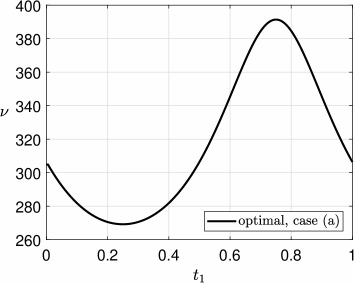
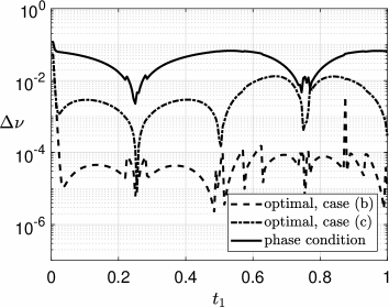
Figure 2: Local frequency function for the optimal solution in case (a) (left) and differences to the local frequency functions of the other cases (right) in three-stage ring oscillator.

node voltage

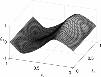
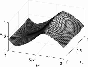
branch current

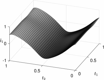
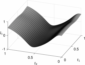
Figure 3: Numerical solutions from method of lines with phase condition (left) and optimality condition (right) for node voltage as well as branch current in three-stage ring oscillator.

Now initial value problems of the DAE systems are solved numerically, as described in Section 5.1, using the computed consistent initial values. Figure 2 (left) shows the local frequency function for the optimal solution in case (a). The modulus of the differences between the other local frequencies and this function are illustrated by Figure 2 (right), where a semi-logarithmic scale is used due to different orders of magnitudes. The phase condition causes the largest difference. Figure 3 depicts the resulting MPDAE solutions for the first node voltage and the first branch current with the phase condition and the optimisation case (a), respectively. We observe that the functions for the phase condition and the optimisation are similar.

5.3 Simulation of eleven-stage ring oscillator

Now the parameters are set to $C=2\cdot 10^{-12}$, $R=10^{3}$, $G=-5$ in the system (44), which includes a more realistic value of the capacitance. A stable periodic solution around 30 MHz emerges for a constant input $b\equiv 1$. We supply the input signal

$$b(t)=1+2\textstyle\sin^{2}\left(\frac{2\pi}{T}t\right)$$

with the forced time rate $T=10^{-4}$ (1 kHz), which causes about 3100 oscillations in the global interval $t\in[0,T]$. As initial values for the associated MPDAE system (18), we take values from an approximation of the stable periodic solution for $b\equiv 1$. Now the dimension reads as $mk+1=2201$ in DAE systems from the method of lines.

We investigate only case (b) of the optimisation and the case of the phase condition (45), where an index-one system and an index-two system, respectively, is guaranteed for sufficiently small step size in the method of lines. We apply the same initial values in both situations. Thus the initial values are just nearly consistent. The slow time scale $t_{1}\in[0,10^{-4}]$ is standardised to $t_{1}\in[0,1]$ in the plots. Figure 4 illustrates the local frequency function of the optimal solution, whereas the relative difference to the local frequencies of the phase condition is in a magnitude of just 0.01%. The multidimensional solutions of the first node voltage as well as the first branch current are shown in Figure 5.

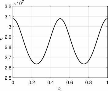
Figure 4: Local frequency function for the optimal solution of case (b) in eleven-stage ring oscillator.

node voltage

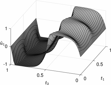
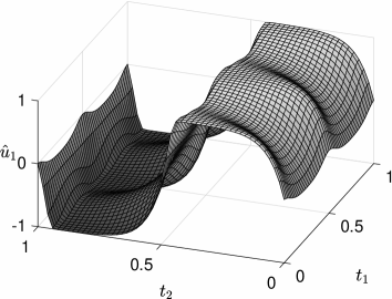
branch current

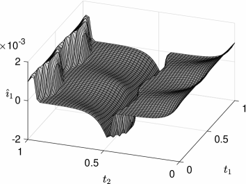
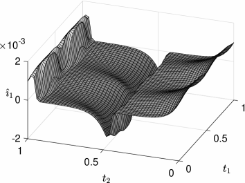
Figure 5: Numerical solutions from method of lines with phase condition (left) and optimality condition (right) for node voltage as well as branch current in eleven-stage ring oscillator.

Finally, we employ the MPDAE solutions to evaluate approximately the functional (7) from the minimisation using the weights of case (b). Figure 6 shows these approximations. Therein, the optimality of the solution obtained by the necessary condition (8) is indicated. Nevertheless, the phase condition (45) yields a suboptimal solution.

We omit the discussion of solutions of the DAE system (44) reconstructed by the MPDAE solutions using (5). Respective numerical results are presented for several test examples in the previous works [24, 27, 31, 34].

         

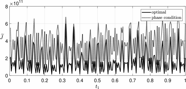
Figure 6: Functional (7) for the optimal solution and for the solution with phase condition in eleven-stage ring oscillator.

6 Conclusions

Initial-boundary value problems of MPDAEs were solved numerically using a method of lines. The resulting system of DAEs includes an additional constraint either from an optimisation or from a phase condition. In the case of semi-explicit DAEs of index one as circuit model, we showed that the differential index of the DAEs increases in several cases determined by the inclusion of either differential variables or algebraic variables in the additional constraint. The necessary condition for an optimal solution including differential variables only is the unique option to keep the index equal to one in the method of lines.

References

- [1] A. Bartel, S. Knorr, R. Pulch, Wavelet-based adaptive grids for multirate partial differential-algebraic equations, Appl. Numer. Math. 59 (2009) 495–506.
- [2] K. Bittner, H.G. Brachtendorf, Adaptive multi-rate wavelet method for circuit simulation, Radioengineering 23 (2014) 300–307.
- [3] K. Bittner, H.G. Brachtendorf, Optimal frequency sweep method in multi-rate circuit simulation, COMPEL 33 (2014) 1189–1197.
- [4] K.E. Brenan, S.L. Campbell, L.R. Petzold, Numerical solution of initial-value problems in differential-algebraic equations. Classics in Applied Mathematics. SIAM, Society for Industrial and Applied Mathematics, 1996.
- [5] H.G. Brachtendorf, G. Welsch, R. Laur, A. Bunse-Gerstner, Numerical steady state analysis of electronic circuits driven by multi-tone signals, Electr. Eng. 79 (1996) 103–112.
- [6] H.G. Brachtendorf, A. Bunse-Gerstner, B. Lang, S. Lampe, Steady state analysis of electronic circuits by cubic and exponential splines, Electr. Eng. 91 (2009) 287–299.
- [7] D. Estévez Schwarz, R. Lamour, Diagnosis of singular points of structured DAEs using automatic differentiation. Numer. Algor. 69 (4) (2015) 667–691.
- [8] D. Estévez Schwarz, R. Lamour, Diagnosis of singular points of properly stated DAEs using automatic differentiation. Numer. Algor. 70 (4) (2015) 777–805.
- [9] D. Estévez Schwarz, R. Lamour, A new projector based decoupling of linear DAEs for monitoring singularities. Numer. Algor. 73 (2) (2016) 535–565.
-
[10]
D. Estévez Schwarz, R. Lamour,
A new approach for computing consistent initial values and Taylor coefficients
for DAEs using projector-based constrained optimization.
Numer. Algor. (2017)
DOI 10.1007/s11075-017-0379-9. - [11] J. Greb, R. Pulch, Simulation of quasiperiodic signals via warped MPDAEs using Houben’s approach, in: G. Ciuprina, D. Ioan (eds.), Scientific Computing in Electrical Engineering SCEE 2006, Mathematics in Industry, Vol. 11, Springer, Berlin, 2007, pp. 237–243.
- [12] E. Griepentrog, R. März, Differential-Algebraic Equations and their Numerical Treatment, Teubner, Leipzig, 1986.
- [13] M. Günther, U. Feldmann, CAD based electric circuit modeling in industry I: mathematical structure and index of network equations, Surv. Math. Ind. 8 (1999) 97–129.
- [14] E. Hairer, S.P. Nørsett, G. Wanner, Solving Ordinary Differential Equations. Vol. 1: Nonstiff Problems, 2nd ed., Springer, Berlin, 1993.
- [15] E. Hairer, G. Wanner, Solving Ordinary Differential Equations. Vol. 2: Stiff and Differential-Algebraic Equations, 2nd ed., Springer, Berlin, 1996.
- [16] C.W. Ho, A. Ruehli, P.A. Brennan, The modified nodal approach to network analysis, IEEE Trans. Circuits and Systems CAS 22 (1975) 504–509.
- [17] S.H.M.J. Houben, Circuits in motion. The numerical simulation of electrical circuits, PhD thesis, Eindhoven University of Technology, The Netherlands, 2003.
- [18] S.H.M.J. Houben, Simulating multi-tone free-running oscillators with optimal sweep following, in: W.H.A. Schilders, E.J.W. ter Maten, S.H.M.J. Houben (eds.), Scientific Computing in Electrical Engineering SCEE 2002, Mathematics in Industry, Vol. 4, Springer, Berlin, 2004, pp. 240–247.
- [19] W. Kampowsky, P. Rentrop, W. Schmitt, Classification and numerical simulation of electric circuits, Surv. Math. Ind. 2 (1992) 23–65.
- [20] B. Kugelmann, R. Pulch, Existence and uniqueness of optimal solutions for multirate partial differential algebraic equations, Appl. Numer. Math. 97 (2015) 69–87.
- [21] P. Kunkel, V. Mehrmann, Differential-Algebraic Equations: Analysis and Numerical Solution, EMS, Zürich, 2006.
- [22] X. Lai, J. Roychowdhury, Capturing oscillator injection locking via nonlinear phase-domain macromodels, IEEE Trans. Microw. Theory Techn. 52 (2004) 2251–2261.
- [23] R. Lamour, R. März, C. Tischendorf, Differential-algebraic equations: A projector based analysis, Differential-Algebraic Equations Forum 1, Springer, Berlin, 2013.
- [24] O. Narayan, J. Roychowdhury, Analyzing oscillators using multitime PDEs, IEEE Trans. CAS I 50 (7) (2003) 894–903.
- [25] J. F. Oliveira, J. C. Pedro, Efficient RF circuit simulation using an innovative mixed time-frequency method, IEEE Trans. Microw. Theory Techn. 59 (4) (2011) 827–836.
- [26] R. Pulch, M. Günther, A method of characteristics for solving multirate partial differential equations in radio frequency applications, Appl. Numer. Math. 42 (1) (2002) 397–409.
- [27] R. Pulch, Multi time scale differential equations for simulating frequency modulated signals, Appl. Numer. Math. 53 (2-4) (2005) 421–436.
- [28] R. Pulch, Warped MPDAE models with continuous phase conditions, in: A. Di Bucchianico, R.M.M. Mattheij, M.A. Peletier (eds.), Progress in Industrial Mathematics at ECMI 2004, Mathematics in Industry, Vol. 8, Springer, Berlin, 2006, pp. 179–183.
- [29] R. Pulch, M. Günther, S. Knorr, Multirate partial differential algebraic equations for simulating radio frequency signals, Euro. Jnl. of Applied Mathematics 18 (2007) 709–743.
- [30] R. Pulch, Multidimensional models for analysing frequency modulated signals, Math. Comp. Modell. Dyn. Syst. 13 (4) (2007) 315–330.
- [31] R. Pulch, Initial-boundary value problems of warped MPDAEs including minimisation criteria, Math. Comput. Simulat. 79 (2) (2008) 117–132.
- [32] R. Pulch, Variational methods for solving warped multirate partial differential algebraic equations, SIAM J. Sci. Comput. 31 (2) (2008) 1016–1034.
- [33] R. Pulch, Transformation qualities of warped multirate partial differential algebraic equations, in: M. Breitner, G. Denk, P. Rentrop (eds.), From Nano to Space - Applied Mathematics Inspired by Roland Bulirsch, Springer, Berlin, 2008, pp. 27–42.
- [34] R. Pulch, B. Kugelmann, DAE-formulation for optimal solutions of a multirate model, Proc. Appl. Math. Mech. 15 (2015) 615–616.
- [35] J. Roychowdhury, Analyzing circuits with widely-separated time scales using numerical PDE methods, IEEE Trans. CAS I 48 (5) (2001) 578–594.
- [36] L.L. Zhu, C.E. Christoffersen, Transient and steady-state analysis of nonlinear RF and microwave circuits, EURASIP Journal on Wireless Communications and Networking, Vol. 2006, Special Issue on CMOS RF Circuits for Wireless Applications, Article ID 32097, 1–11.