Power Control for Multi-Cell Networks with Non-Orthogonal Multiple Access

Abstract

In this paper, we investigate the problems of sum power minimization and sum rate maximization for multi-cell networks with non-orthogonal multiple access. Considering the sum power minimization, we obtain closed-form solutions to the optimal power allocation strategy and then successfully transform the original problem to a linear one with a much smaller size, which can be optimally solved by using the standard interference function. To solve the nonconvex sum rate maximization problem, we first prove that the power allocation problem for a single cell is a convex problem. By analyzing the Karush-Kuhn-Tucker conditions, the optimal power allocation for users in a single cell is derived in closed form. Based on the optimal solution in each cell, a distributed algorithm is accordingly proposed to acquire efficient solutions. Numerical results verify our theoretical findings showing the superiority of our solutions compared to the orthogonal frequency division multiple access and broadcast channel.

I Introduction

With the explosive growth of data traffic in mobile Internet [1], non-orthogonal multiple access (NOMA) has been recently proposed [2, 3]. By using superposition coding at the transmitter and successive interference cancelation (SIC) at the receiver, NOMA can achieve higher spectral efficiency than conventional orthogonal multiple access, such as orthogonal frequency division multiple access (OFDMA). Besides, NOMA can support more connections by letting more than one user simultaneously access the same frequency or time resources [4, 5, 6, 7]. Therefore, NOMA has been deemed as a promising multiple access scheme for the next generation mobile communication networks [8, 9, 10].

NOMA can simultaneously serve multiple users with the same frequency band and time slot by splitting them in the power domain [11]. The basic concept of NOMA with SIC receiver was introduced in [12]. The ergodic sum rate and the outage performance with fixed power allocation were analyzed in [13] for NOMA. Specific impacts of power allocation on sum rate [14, 15, 16], fairness [17, 18, 19], and energy efficiency [20, 21] were investigated. Moreover, joint sub-channel and power allocation was studied in [22, 23, 24, 25, 26]. However, the above existing works [12, 13, 14, 15, 16, 17, 18, 19, 20, 22, 23, 24, 25, 26, 21] are limited to single-cell analysis, where there is no inter-cell interference.

Recently, NOMA has been extended to multi-cell networks [27, 28, 29, 30, 31, 32, 33]. Different from multi-cell networks with OFDMA, users in the same cell can receive intra-cell interference, which can be subtracted by using SIC in multi-cell networks with NOMA. Different from single-cell networks with NOMA, inter-cell interference should be considered in multi-cell networks with NOMA. To harness the effect of inter-cell interference, joint processing (JP) and coordinated scheduling (CS) technologies are usually adopted [34]. In NOMA-JP, the users’ data symbols are available at more than one base station (BS) [27]. The designs of CS for NOMA differ from those of JP in that the users’ data are not shared among the BSs [28]. However, the cooperating BSs in NOMA-CS still need to exchange global channel state information and cooperative scheduling information via a standardized interface named X2. In addition, the number of transmission points is one for NOMA-CS [28], while the number of transmission points is more than one for NOMA-JP in [27]. Moreover, the numbers of supported users by NOMA-CS and NOMA-JP are different [29].

Based on NOMA-CS, the uplink and downlink power control problems for sum power minimization in two-cell networks with NOMA were studied in [31] and [32], respectively. However, the above existing works [30, 27, 32, 31] were merely limited to power minimization in a two-cell network with only two users per cell. The sum rate maximization problem in multiple-input multiple-output (MIMO)-NOMA multi-cell networks was investigated in [33], where two users are paired in a virtual cluster. Consequently, there is a lack of systematic approach for sum power minimization and sum rate maximization problems via power control in multi-cell networks with NOMA from a mathematical optimization point of view.

The objective of this paper is to investigate the power control problems for sum power minimization and sum rate maximization in multi-cell networks with NOMA. The contributions of this paper are summarized as follows:

1. The sum power minimization problem can be equivalently transformed into a linear problem (LP) with smaller variables. Having obtained the total transmission power of all BSs, the power allocation for each user can be presented in a closed-form expression.

2. To solve the sum rate maximization problem, we decouple it into two subproblems, i.e., power allocation problem for users in a single cell and power control problem in multiple cells. With the total transmission power of all BSs fixed, we succeed in showing that power control problem in a single cell is a convex problem. By analyzing the Karush-Kuhn-Tucker (KKT) conditions, we observe that only the user with the highest channel gain deserves additional power allocation, while the power for other users in the same cell is merely determined to maintain their minimal rate demands. Closed-form expressions of the optimal power allocation and optimal sum rate in a single cell are further obtained.

3. Based on the closed-form expression of the optimal sum rate in a single cell, the original sum rate maximization problem can be equivalently transformed into a simplified problem. Since the objective function for each BS can be formulated as a difference of two convex functions (DC), a convex approximation of the objective function is introduced. Furthermore, a distributed algorithm is also provided to obtain a suboptimal solution.

The rest of the paper is organized as follows. In Section II, we introduce the system model and power control formulation. Sum power minimization and sum rate maximization for multi-cell networks with NOMA are addressed in Section III and Section IV, respectively. The extension to MIMO-NOMA systems is introduced in Section V. Some numerical results are shown in Section VI and conclusions are finally drawn in Section VII.

II System Model and Problem Formulation

Consider a downlink multi-cell network with NOMA, where there are $I$ BSs and $J$ users. Denote the set of BSs and users by ${\mathcal{I}}=\{1,2,\cdots,I\}$ and ${\mathcal{J}}=\{1,2,\cdots,J\}$, respectively. The unique group of users served by BS $i\in{\mathcal{I}}$ is denoted by set ${\cal{J}}_{i}=\{J_{i-1}+1,J_{i-1}+2,\cdots,J_{i}\}$, where $J_{0}=0$, $J_{I}=J$, $J_{i}=\sum_{l=1}^{i}|{\cal{J}}_{l}|$, and $|\cdot|$ is the cardinality of a set. We focus on the downlink where mutual interference exists among cells.

By using NOMA, a BS serves multiple users by splitting them in the power domain. Assume that each BS shares the same spectrum. For each BS, the total bandwidth, $B_{\text{total}}$ is equally divided into $M$ subchannels, where the bandwidth of each subchannel is $B=B_{\text{total}}/M$. Let $\mathcal{M}=\{1,2,\cdots,M\}$ be the set of subchannels. The set of users served by BS $i$ on subchannel $m$ is denoted by $\mathcal{J}_{im}=\{J_{i(m-1)}+1,J_{i(m-1)}+2,\cdots,J_{im}\}$, where $J_{i0}=J_{i-1}+1$, $J_{iM}=J_{i}$, $J_{im}=\sum_{l=1}^{m}|\mathcal{J}_{il}|$ and $|{\cal{J}}_{il}|\geq 2$. The channel gain between BS $i$ and user $j\in\mathcal{J}_{im}$ on subchannel $m$ is denoted by $h_{ijm}$. Without loss of generality, the channels are sorted as $|h_{i(J_{i(m-1)}+1)m}|\leq|h_{i(J_{i(m-1)}+2)m}|\leq\cdots\leq|h_{iJ_{im}m}|$, $\forall i\in\mathcal{I}$, $m\in\mathcal{M}$. According to the NOMA principle, BS $i$ simultaneously transmits signal $s_{im}$ to all its served users in $\mathcal{J}_{im}$. The transmitted signal $s_{im}$ can be expressed as

$$s_{im}=\sum_{j=J_{i(m-1)}+1}^{J_{im}}\sqrt{p_{ijm}}s_{ijm},$$ (1)

where $s_{ijm}$ and $p_{ijm}$ are the message and allocated power for user $j\in\mathcal{J}_{im}$, respectively.

The observation at user $j\in\mathcal{J}_{im}$ on subchannel $m$ is given by

$$y_{ijm} \!\!\!\!\!\!\!\!\!\!\!=h_{ijm}s_{im}+\sum_{k\in\mathcal{I}\setminus\{i\}}h_{kjm}s_{km}+n_{jm}$$ (2)

$$\!\!\!\!\!\!\!\!\!\!\!=\sum_{l=J_{i(m-1)}+1}^{J_{im}}h_{ijm}\sqrt{p_{ilm}}s_{ilm}$$

$$\!\!\!\!\!\!\!\!\!\!\!+\sum_{k\in\mathcal{I}\setminus\{i\}}\sum_{n=J_{k(m-1)}+1}^{J_{km}}h_{kjm}\sqrt{p_{knm}}s_{knm}+n_{jm},$$

where $h_{kjm}$ is the cross channel gain between BS $k$ and user $j$ served by BS $i$ on subchannel $m$, and $n_{jm}$ represents the additive zero-mean Gaussian noise with variance $\sigma^{2}$. According to [12, 13, 14, 15], each user should decode the messages of other users in the same cell with lower channel gains before decoding its own message. Denoting the total transmission power of BS $i$ on subchannel $m$ by $q_{im}=\sum_{j=J_{i(m-1)}+1}^{J_{im}}p_{ijm}$, the achievable rate of user $j\in\mathcal{J}_{im}$ to detect the message of user $l\in\{J_{i(m-1)}+1,\cdots,j\}$ on subchannel $m$ is

$$r_{ijlm}=B\log_{2}\left(1+\frac{|h_{ijm}|^{2}p_{ilm}}{|h_{ijm}|^{2}\sum_{n=l+1}^{J_{im}}p_{inm}+Z_{ijlm}}\right),$$ (3)

where

$$Z_{ijlm}=\sum_{k\in\mathcal{I}\setminus\{i\}}q_{km}|h_{kjm}|^{2}+\sigma^{2}.$$ (4)

According to (3), strong user $j$ with high channel gain needs to decode the message of weak user $l\leq j$ with low channel gain. To ensure successful SIC, the achievable rate of user $j\in\mathcal{J}_{im}$ on subchannel $m$ can be given by

$$r_{ijm} \!\!\!\!\!\!\!\!\!=\min_{l\in\{j,\cdots,J_{im}\}}r_{iljm}$$ (5)

$$\!\!\!\!\!\!\!\!\!=\min_{l\in\{j,\cdots,J_{im}\}}B\log_{2}\left(1+\frac{p_{ijm}}{\sum_{n=j+1}^{J_{im}}p_{inm}+\frac{Z_{iljm}}{|h_{ilm}|^{2}}}\right)$$

$$\!\!\!\!\!\!\!\!\!=B\log_{2}\left(1+\frac{p_{ijm}}{\sum_{n=j+1}^{J_{im}}p_{inm}+H_{ijm}}\right),$$

where

$$H_{ijm}=\max_{l\in\{j,\cdots,J_{im}\}}\frac{\sum_{k\in\mathcal{I}\setminus\{i\}}q_{km}|h_{klm}|^{2}+\sigma^{2}}{|h_{ilm}|^{2}}.$$ (6)

Denote $R_{ijm}>0$ as the minimal rate demand of user $j\in\mathcal{J}_{im}$ on subchannel $m$. Applying (5), $r_{ijm}\geq R_{ijm}$ is equivalent to the following linear constraint:

$$p_{ijm}\geq\left(2^{\frac{R_{ijm}}{B}}-1\!\right)\left(\sum_{n=j+1}^{J_{im}}p_{inm}+H_{ijm}\right).$$ (7)

Our objective is to optimize the power allocation in order to minimize the sum power or maximize the sum rate under the total power constraints and individual rate demands. Mathematically, the power control problem can be formulated as

$$\mathop{\min}_{\boldsymbol{p}\geq\boldsymbol{0},\boldsymbol{q}\geq\boldsymbol{0}}\;\quad V(\boldsymbol{p},\boldsymbol{q})$$ (8a)

s.t. $$q_{im}=\sum_{j=J_{i(m-1)}+1}^{J_{im}}p_{ijm},\quad\forall i\in\mathcal{I},m\in\mathcal{M}$$ (8b)

$$p_{ijm}\geq\left(2^{\frac{R_{ijm}}{B}}-1\!\right)\left(\sum_{n=j+1}^{J_{im}}p_{in}+H_{ijm}\right),$$

$$\qquad\forall i\in\mathcal{I},m\in\mathcal{M},j\in\mathcal{J}_{im}$$ (8c)

$$\sum_{m=1}^{M}q_{im}\leq Q_{i},\quad\forall i\in\mathcal{I},$$ (8d)

where $\boldsymbol{p}=[p_{111},\cdots,p_{1J_{1M}{M}},\cdots,p_{IJ_{IM}M}]^{T}$ is the transmission power vector, $\boldsymbol{q}=[q_{11},\cdots,$ $q_{1M},\cdots,q_{IM}]^{T}$ is the total transmission power vector, $H_{ijm}$ is defined in (6), and $Q_{i}$ is the maximum transmission power of the BS $i$. Constraints (8c) reflect that the minimal rate demands of all users can be satisfied. $V(\boldsymbol{p},\boldsymbol{q})$ is the objective function, which can be sum power $\sum_{i=1}^{I}\sum_{m=1}^{M}q_{im}$ or negative sum rate $-\sum_{i=1}^{I}\sum_{m=1}^{M}\sum_{j=J_{i(m-1)}+1}^{J_{im}}r_{ijm}$ with $r_{ijm}$ defined in (5).

Obviously, the feasible set of Problem (8) is linear. For sum power minimization, Problem (8) is a LP, of which the globally optimal solution can be effectively obtained. In the following, we show that sum power minimization problem can be equivalently transformed into a smaller LP. Since the problem of sum rate maximization problem is nonconvex, obtaining global optimum however is known to be difficult. To solve the sum rate maximization problem efficiently, we first consider the power allocation problem for users in a single cell with fixed total transmission power of all BSs. Then, based on the optimal power allocation for users in a single cell, the primal multi-cell sum rate maximization problem can also be simplified into an equivalent problem. A distributed algorithm is proposed to obtain a suboptimal solution of the simplified sum rate maximization problem.

III Sum Power Minimization for Multi-Cell Networks

In this section, we solve the sum power minimization Problem (8) with

$$V(\boldsymbol{p},\boldsymbol{q})=\sum_{i=1}^{I}\sum_{m=1}^{M}q_{im}.$$ (9)

Obviously, sum power minimization Problem (8) is a LP. According to (7), the interference level received by each user is determined by total transmission power $\boldsymbol{q}$. Once the total transmission power of other BSs is given, Problem (8) with objective function (9) can be simplified to a single-cell power minimization problem with fixed inter-cell interference, which fortunately has closed-form solution. Substituting the closed-form solution for each cell into Problem (8), we can obtain an equivalent LP with a much smaller size, i.e., far fewer variables.

III-A Distributed Power Control Algorithm

Theorem 1

For sum power minimization Problem (8) with objective function (9), power $\boldsymbol{p}$ can be optimally solved with closed-form expression as

$$p_{ijm} \!\!\!\!\!\!\!\!\!\!\!=\sum_{n=j}^{J_{im}}{\left(2^{\frac{R_{inm}}{B}}-1\right){2^{\sum_{s=j}^{n-1}\frac{R_{ism}}{B}}}H_{inm}}$$ (10)

$$\!\!\!\!\!\!\!\!\!\!\!\quad-\sum_{n=j+1}^{J_{im}}{\left(2^{\frac{R_{inm}}{B}}\!-\!1\!\right){2^{\sum_{s=j+1}^{n-1}\frac{R_{ism}}{B}}}H_{inm}},$$

while the optimal solution to $\boldsymbol{q}$ (for determining $H_{inm}$) is determined by solving a smaller LP in (11) with much lower complexity.

$$\mathop{\min}_{\boldsymbol{q}\geq\boldsymbol{0}}\;\quad \sum_{i=1}^{I}\sum_{m=1}^{M}q_{im}$$ (11a)

s.t. $$q_{im}\geq\sum_{j=J_{i(m-1)}+1}^{J_{im}}\left(2^{\frac{R_{ijm}}{B}}-1\right){2^{\sum_{s=J_{i(m-1)}+1}^{j-1}\frac{R_{ism}}{B}}}$$

$$\qquad\!\!\!\!\!\!\!\max_{l\in\{j,\cdots,J_{im}\}}\frac{\sum_{k\in\mathcal{I}\setminus\{i\}}q_{km}|h_{klm}|^{2}+\sigma^{2}}{|h_{ilm}|^{2}}$$

$$\qquad\!\!\!\!\!\!\!\>\;\triangleq f_{im}(\boldsymbol{q}),\quad\forall i\in\mathcal{I},m\in\mathcal{M}$$ (11b)

$$\sum_{m=1}^{M}q_{im}\leq Q_{i},\quad\forall i\in\mathcal{I}.$$ (11c)

Proof: Please refer to Appendix A. $\Box$

Note that the concept of strong user reflected from (3), (5) and (6) is helpful in obtaining the closed-form expression in (10). It can be verified that the optimal solution to LP (11) with given $[q_{1m},\cdots,q_{(i-1)m},q_{(i+1)m},\cdots,q_{Im}]^{T}$ can be directly obtained by $q_{im}=f_{im}(\boldsymbol{q})$. To solve LP (11) for multi-cell power minimization, we provide a distributed algorithm in Algorithm 1.

Algorithm 1 Distributed Power Control for Sum Power Minimization (DPC-SPM)

1:Initialize $q_{im}^{(0)}=Q_{i}/M$, $\forall i\in\mathcal{N},m\in\mathcal{M}$. Set $t=1$, and maximal iteration number $T_{\max}$.

2:for $i=1,2,\cdots,I$ do

3:     for $m=1,2,\cdots,M$ do

4:         Calculate $q_{im}^{(t)}=f_{im}(\boldsymbol{q}^{(t-1)})$;

5:     end for

6:end for

7:If $t>T_{\max}$ or objective function (11a) converges, output $\boldsymbol{q}^{*}=\boldsymbol{q}^{(t)}$, and terminate. Otherwise, $\boldsymbol{q}^{(t)}=[q_{11}^{(t)},\cdots,q_{1M}^{(t)},\cdots,q_{IM}^{(t)}]^{T}$, set $t=t+1$ and go to step 2.

III-B Convergence and Global Optimality

To show the convergence and global optimality of DPC-SPM algorithm, we recap the standard interference function introduced in [35]. Letting $\boldsymbol{f}=[f_{11},\cdots,f_{IM}]^{T}$, we have the following theorem.

Theorem 2

$\boldsymbol{f}(\boldsymbol{q})$ is a standard interference function.

Proof: Please refer to Appendix B. $\Box$

Based on Theorem 2, we have the following corollaries.

Corollary 1

If there exists $\boldsymbol{q}$ such that $\boldsymbol{q}\geq\boldsymbol{f}(\boldsymbol{q})$, the iterative fixed-point method $\boldsymbol{q}^{(t+1)}=\boldsymbol{f}(\boldsymbol{q}^{(t)})$ will converge to the unique fixed point $\boldsymbol{q}^{*}=\boldsymbol{f}(\boldsymbol{q}^{*})$ with any initial point $\boldsymbol{q}^{(0)}$.

Proof: Please refer to [35, Theorem 2]. $\Box$

Corollary 2

If Problem (11) is feasible, the optimal $\boldsymbol{q}^{*}$ of Problem (11) is component-wise minimum in the sense that any other feasible solution $\boldsymbol{q}^{\prime}$ that meets constraints (11b)-(11c) and $\boldsymbol{q}^{\prime}\geq\boldsymbol{0}$ satisfying $\boldsymbol{q}^{\prime}\geq\boldsymbol{q}^{*}$.

Corollary 3

Problem (11) is feasible, if and only if there exists $\boldsymbol{q}^{*}=\boldsymbol{f}(\boldsymbol{q}^{*})$ and $\sum_{m=1}^{M}q_{im}^{*}\leq Q_{i},\forall i\in\mathcal{I}$. If Problem (11) is feasible, the optimal solution $\boldsymbol{q}^{*}$ to Problem (11) is unique with satisfying $\boldsymbol{q}^{*}=\boldsymbol{f}(\boldsymbol{q}^{*})$.

Since Corollary 2 and 3 can be easily proved by using the same method in [35, Theorem 2], the proofs are omitted. From Corollary 1 to Corollary 3, the convergence and global optimality of DPC-SPM algorithm can be verified.

III-C Further Discussion

Considering the special case where users in the same cell on the same subchannel are with equal rate demands, i.e., $R_{i(J_{i(m-1)}+1)}=\cdots=R_{iJ_{im}}=R_{im}$, we show that user with poor channel should be allocated with more power than user with better channel in the same cell, i.e., $p_{i(J_{i(m-1)}+1)m}>\cdots>p_{iJ_{im}m}$. From (10), for all $J_{i(m-1)}+2\leq j\leq J_{im}$, it is verified that:

$$p_{i(j-1)m}-p_{ijm}=\sum_{n=j-1}^{J_{im}}\left(2^{\frac{R_{im}}{B}}-1\right)2^{\frac{(n-j+1)R_{im}}{B}}H_{inm}$$

$$\quad+\sum_{n=j+1}^{J_{im}}\left(2^{\frac{R_{im}}{B}}-1\right)2^{\frac{(n-j-1)R_{im}}{B}}H_{inm}$$

$$\quad-2\sum_{n=j}^{J_{im}}\left(2^{\frac{R_{im}}{B}}-1\right)2^{\frac{(n-j)R_{im}}{B}}H_{inm}$$

$$=\!\sum_{n=j}^{J_{im}}\left(2^{\frac{R_{im}}{B}}\!-\!1\right)2^{\frac{(n-j+1)R_{im}}{B}}H_{inm}\!+\!\left(2^{\frac{R_{im}}{B}}\!-\!1\right)H_{i(j-1)m}$$

$$\quad\!-\!\!\left(\!2^{\frac{R_{im}}{B}}\!-\!1\!\right)\!\!2^{\frac{-R_{im}}{B}}\!H_{ijm}\!+\!\sum_{n=j}^{J_{im}}\!\left(\!2^{\frac{R_{im}}{B}}\!-\!1\!\right)\!\!2^{\frac{(n-j-1)R_{im}}{B}}\!H_{inm}$$

$$\quad-2\sum_{n=j}^{J_{im}}\left(2^{\frac{R_{im}}{B}}-1\right)2^{\frac{(n-j)R_{im}}{B}}H_{inm}$$

$$>\sum_{n=j}^{J_{im}}{\left(2^{\frac{R_{im}}{B}}-1\right)2^{\frac{(n-j)R_{im}}{B}}}\left(2^{\frac{R_{im}}{B}}+2^{\frac{-R_{im}}{B}}-2\right)H_{inm}$$

$$>0,$$

where the first inequality follows from

$$\!\!\!\!\!\!\!\!\!\!\!H_{i(j-1)m}=\max_{l\in\{j-1,\cdots,J_{im}\}}\frac{\sum_{k\in\mathcal{I}\setminus\{i\}}q_{km}|h_{klm}|^{2}+\sigma^{2}}{|h_{ilm}|^{2}}$$

$$\!\!\!\!\!\!\!\!\!\!\!\quad\geq\max_{l\in\{j,\cdots,J_{im}\}}\frac{\sum_{k\in\mathcal{I}\setminus\{i\}}q_{km}|h_{klm}|^{2}+\sigma^{2}}{|h_{ilm}|^{2}}=H_{ijm}$$ (12)

and $2^{\frac{R_{im}}{B}}>1$, and the second inequality holds because $x+x^{-1}>2$ for $x>1$ and $0<x<1$.

To implement the NOMA scheme, each BS broadcasts the channel gain orders and the cancellation schemes to all served users. The weakest user directly decodes its own message. With the help of SIC, the strong user decodes the messages in two stages. In the first stage, the strong user needs to decode the messages of weak users served by the same BS on the same subchannel. In the next stage, the strong user subtracts the decoded messages and then decodes its own message. For OFDMA and broadcast channel (BC), each user only needs to decode its own message, i.e., all users do not need to conduct SIC. Thus, for NOMA, the BSs need to broadcast additional information to assist SIC of the users and the receivers are complicated compared with OFDMA and BC.

IV Sum Rate Maximization for Multi-Cell Networks

In this section, we solve the sum rate maximization Problem (8) with

$$V(\boldsymbol{p},\boldsymbol{q})=-\sum_{i=1}^{I}\sum_{m=1}^{M}\sum_{j=J_{i(m-1)}+1}^{J_{im}}r_{ijm}.$$ (13)

For sum rate maximization Problem (8), we show that it can be decoupled into two subproblems, i.e., power allocation problem in a single cell, and power control problem in multiple cells. Given total transmission power $\boldsymbol{q}$, inter-cell interference can be evaluated as constant value, hence the sum rate maximization Problem (8) can be further decoupled into multiple single-cell power allocation problems. The power allocation problem in a single cell can be proved to be convex by checking the convexity of the objective function. By solving the KKT conditions, the closed-form expression of power allocation problem in a single cell can be obtained. Based on the results of power allocation problem in a single cell, the original sum rate maximization Problem (8) can be transformed into an equivalent problem with fewer variables. A distributed algorithm is proposed to solve the transformed problem.

With given total transmission power $\boldsymbol{q}$, sum rate maximization Problem (8) with objective function (13) becomes the following problem,

$$\mathop{\min}_{\boldsymbol{p}\geq\boldsymbol{0}}\; -\sum_{i=1}^{I}\!\sum_{m=1}^{M}\!\sum_{j=J_{i(m-1)}+1}^{J_{im}}\!B\log_{2}\left(\!1\!+\!\frac{p_{ijm}}{\sum\limits_{n=j+1}^{J_{im}}\!p_{inm}\!+\!H_{ijm}}\!\right)$$ (14a)

s.t. $$\sum_{j=J_{i(m-1)}+1}^{J_{im}}p_{ijm}=q_{im},\quad\forall i\in\mathcal{I},m\in\mathcal{M}$$ (14b)

$$p_{ijm}\geq\left(2^{\frac{R_{ijm}}{B}}-1\right)\left(\sum_{n=j+1}^{J_{im}}p_{inm}+H_{ijm}\right),$$

$$\qquad\forall i\in\mathcal{I},m\in\mathcal{M},j\in\mathcal{J}_{im}.$$ (14c)

Since Problem (14) has a decoupling objective function and decoupling constraints, Problem (14) can be decoupled into $IM$ individual problems. Having solved the $IM$ individual problems, we can substitute those $IM$ optimal solutions into Problem (8), which results in the power control problem in multiple cells. Thus, the original Problem (8) can be decoupled into power allocation problem in a single cell and power control problem in multiple cells.

IV-A Power Allocation in A Single Cell

For Problem (14), power allocation problem for BS $i$ on subchannel $m$ is formulated as

$$\mathop{\min}_{\boldsymbol{p}_{im}\geq\boldsymbol{0}}\; -\sum_{j=J_{i(m-1)}+1}^{J_{im}}B\log_{2}\left(1+\frac{p_{ijm}}{\sum_{n=j+1}^{J_{im}}p_{inm}+H_{ijm}}\right)$$ (15a)

s.t. $$\sum_{j=J_{i(m-1)}+1}^{J_{im}}p_{ijm}=q_{im}$$ (15b)

$$p_{ijm}\geq\left(2^{\frac{R_{ijm}}{B}}-1\right)\left(\sum_{n=j+1}^{J_{im}}p_{inm}+H_{ijm}\right),$$

$$\qquad\forall j\in\mathcal{J}_{im},$$ (15c)

where $\boldsymbol{p}_{im}=[p_{i(J_{i(m-1)}+1)m},\cdots,p_{iJ_{im}m}]^{T}$.

Since the convexity of objective function (15a) cannot be easily checked, the sum rate maximization problem was regarded as a nonconvex multivariate optimization problem via nonlinear programming approaches [20, 22]. To solve Problem (15), we show that Problem (15) is indeed convex by checking the convexity of objective function (15a).

Theorem 3

Problem (15) is a convex problem, and there exists at least one feasible solution to Problem (15) if and only if the total transmission power of BS $i$ and rate constraints of users served by BS $i$ satisfy the following condition:

$$\sum_{j=J_{i(m-1)}+1}^{J_{im}}{\left(2^{\frac{R_{ijm}}{B}}-1\right)}{2^{\sum_{s=J_{i(m-1)}+1}^{j-1}\frac{R_{ism}}{B}}}H_{ijm}\leq q_{im}.$$ (16)

Proof: Please refer to Appendix C. $\Box$

Due to that Problem (15) is convex, we can obtain the globally optimal solution by solving the KKT conditions [36, 37], and the following theorem is hence provided.

Theorem 4

The optimal power allocation strategy for each BS is to allocate additional power to the user with the best channel gain, while other users served by this BS are allocated with minimal power to maintain their minimal rate demands. More specifically, the globally optimal power allocation for Problem (15) equals

$$\!\!\!\!\!p_{ijm}\!\!=\!\!\begin{cases}\frac{q_{im}\!\left(2^{\frac{R_{ijm}}{B}}\!-\!1\right)}{2^{\sum_{n\!=\!J_{i(m-1)}\!+\!1}^{j}\!\frac{R_{inm}}{B}}}\!+\!\frac{\left(\!2^{\frac{R_{ijm}}{B}}\!-\!1\!\right)\!H_{ijm}}{2^{\frac{R_{ijm}}{B}}}-\\ \sum_{n=J_{i(m-1)}+1}^{j-1}\!\frac{\left(\!2^{\frac{R_{ijm}}{B}}\!-\!1\!\right)\!\!\left(\!2^{\frac{R_{inm}}{B}}\!-\!1\!\right)\!H_{inm}}{2^{\sum_{l=n}^{j}\frac{R_{ilm}}{B}}},&\!\!\!\!\!\!\mbox{ if $j<J_{im}$}\\ \frac{q_{im}}{2^{\sum_{n=J_{i(m-1)}+1}^{J_{im}-1}\frac{R_{inm}}{B}}}-\\ \sum_{n=J_{i(m-1)}+1}^{J_{im}-1}\frac{\left(2^{\frac{R_{inm}}{B}}-1\right)H_{inm}}{2^{\sum_{l=n}^{J_{im}-1}\frac{R_{ilm}}{B}}},&\!\!\!\!\!\!\mbox{ if $j=J_{im}$}\end{cases},\!\!\!\!\!$$ (17)

and the corresponding optimal value of Problem (15) is

$$-B\log_{2} \!\!\!\!\!\!\!\!\!\!\!\left(1+\frac{q_{im}}{2^{\sum_{j=J_{i(m-1)}+1}^{J_{im}-1}\frac{R_{ijm}}{B}}H_{iJ_{im}m}}-\sum_{j=J_{i(m-1)}+1}^{J_{im}-1}\right.$$ (18)

$$\!\!\!\!\!\!\!\!\!\!\!\left.\frac{\left(2^{\frac{R_{ijm}}{B}}-1\right)H_{ijm}}{2^{\sum_{l=j}^{J_{im}-1}\frac{R_{ilm}}{B}}H_{iJ_{im}m}}\right)-\sum_{j=J_{i(m-1)}+1}^{J_{im}-1}R_{ijm},$$

where the first term is the negative rate of user $J_{im}$ with the largest channel gain among users served by BS $i$ on subchannel $m$, and the second term is the negative sum rate of all other users served by BS $i$ on subchannel $m$.

Proof: Please refer to Appendix D. $\Box$

Similar to (10), the concept of strong user reflected from (3), (5) and (6) is helpful in obtaining the closed-form expression in (17). Especially, the decreasing order of $H_{ijm}$ in (III-C) obtained from (6) is crucial in proving that Problem (15) is convex, which fortunately has closed-form solution. According to (18), we can find that the optimal sum rate is mainly determined by the rate of user $J_{im}$ with best channel gain among users served by BS $i$ on subchannel $m$ and the optimal sum rate increases with the total transmission power of BS $i$ on subchannel $m$ on a logarithmic scale. Note that we obtain the similar conclusion as in [16]. The difference is that the inter-cell interference is not considered in [16].

IV-B Power Control in Multiple Cells

Based on Theorem 3 and Theorem 4, we can readily transform sum rate maximization Problem (8) with objective function (13) into an equivalent problem.

Theorem 5

Sum rate maximization Problem (8) with objective function (13) is equivalent to the following problem:

$$\mathop{\min}_{\boldsymbol{q}\geq\boldsymbol{0},\boldsymbol{x}\geq\boldsymbol{0}}\;\quad \!-\!\sum_{i=1}^{I}\sum_{m=1}^{M}B\left(\!1\!+\!\frac{q_{im}}{2^{\sum_{j=J_{i(m-1)}+1}^{J_{im}-1}\frac{R_{ijm}}{B}}x_{iJ_{im}m}}\right.$$

$$\left.\quad-\sum_{j=J_{i(m-1)}+1}^{J_{im}-1}\frac{\left(2^{\frac{R_{ijm}}{B}}-1\right)x_{ijm}}{2^{\sum_{l=j}^{J_{im}-1}\frac{R_{ilm}}{B}}x_{iJ_{im}m}}\!\right)$$ (19a)

s.t. $$q_{im}\geq\sum_{j=J_{i(m-1)}+1}^{J_{im}}{\left(2^{\frac{R_{ijm}}{B}}-1\right)}$$

$$\qquad{2^{\sum_{s=J_{i(m-1)}+1}^{j-1}\frac{R_{ism}}{B}}}x_{ijm},\quad\forall i\in\mathcal{I},m\in\mathcal{M}$$ (19b)

$$x_{ijm}\geq\frac{\sum_{k\in\mathcal{I}\setminus\{i\}}q_{km}|h_{klm}|^{2}+\sigma^{2}}{|h_{ilm}|^{2}},$$

$$\qquad\forall i\in\mathcal{I},m\in\mathcal{M},j\in\mathcal{J}_{im},{l\in\{j,\cdots,J_{im}\}}$$ (19c)

$$\sum_{m=1}^{M}q_{im}\leq Q_{i},\quad\forall i\in\mathcal{I},$$ (19d)

where $\boldsymbol{x}=[x_{111},\cdots,x_{1J_{1M}{M}},\cdots,x_{IJ_{IM}M}]^{T}$ and the power for each user is given by (17).

Note that there always exists $l\in\{j,\cdots,J_{im}\}$ such that $x_{ijm}=\frac{\sum_{k\in\mathcal{I}\setminus\{i\}}q_{km}|h_{klm}|^{2}+\sigma^{2}}{|h_{ilm}|^{2}}$ for all $i\in\mathcal{I},m\in\mathcal{M},j\in\mathcal{J}_{im}$ as the objective function increases with $x_{ijm}$, which shows that $x_{ijm}=H_{ijm}$ defined in (6). Since Theorem 5 can be easily proved through substituting (17) into Problem (8) with objective function (13), the proof of Theorem 5 is omitted. It can be found that the objective function in Problem (19) is still nonconvex and the constraints of Problem (19) are all linear with respect to $\boldsymbol{q}$ and $\boldsymbol{x}$. In the following, one distributed algorithm with low complexity is proposed. Denote $\boldsymbol{q}_{i}=[q_{i1},\cdots,q_{iM}]^{T}$ and $\boldsymbol{x}_{i}=[x_{i(J_{i0}+1)1},\cdots,x_{iJ_{iM}M}]^{T}$. With given $\boldsymbol{q}_{-i}=[\boldsymbol{q}_{1}^{T},\cdots,\boldsymbol{q}_{i-1}^{T},\boldsymbol{q}_{i+1}^{T},\cdots,\boldsymbol{q}_{I}^{T}]^{T}$ and $\boldsymbol{x}_{-i}=[\boldsymbol{x}_{1}^{T},\cdots,\boldsymbol{x}_{i-1}^{T},\boldsymbol{x}_{i+1}^{T},\cdots,\boldsymbol{x}_{I}^{T}]^{T}$, Problem (19) becomes the following optimization problem for BS $i$,

$$\mathop{\min}_{\boldsymbol{q}_{i}\geq\boldsymbol{0},\boldsymbol{x}_{i}\geq\boldsymbol{0}}\;\quad -\sum_{m=1}^{M}B\left(1+\frac{q_{im}}{2^{\sum_{j=J_{i(m-1)}+1}^{J_{im}-1}\frac{R_{ijm}}{B}}x_{iJ_{im}m}}\right.$$

$$\left.\quad-\sum_{j=J_{i(m-1)}+1}^{J_{im}-1}\frac{\left(2^{\frac{R_{ijm}}{B}}-1\right)x_{ijm}}{2^{\sum_{l=j}^{J_{im}-1}\frac{R_{ilm}}{B}}x_{iJ_{im}m}}\right)$$ (20a)

s.t. $$q_{im}\geq\sum_{j=J_{i(m-1)}+1}^{J_{im}}{\left(2^{\frac{R_{ijm}}{B}}-1\right)}$$

$$\qquad{2^{\sum_{s=J_{i(m-1)}+1}^{j-1}\frac{R_{ism}}{B}}}x_{ijm},\quad m\in\mathcal{M}$$ (20b)

$$x_{ijm}\geq H_{ijm},\quad\forall m\in\mathcal{M},j\in\mathcal{J}_{im}$$ (20c)

$$q_{im}\leq Q_{im},\quad\forall m\in\mathcal{M}$$ (20d)

$$\sum_{m=1}^{M}q_{im}\leq Q_{i},$$ (20e)

where $H_{ijm}$ is defined in (6), and constraints (20d) follow from (19c) with

$$Q_{im}= \!\!\!\!\!\!\!\!\!\!\!\min_{n\in\mathcal{N}\setminus\{i\},j\in\mathcal{J}_{nm},l\in\{j,\cdots,J_{nm}\}}$$ (21)

$$\!\!\!\!\!\!\!\!\!\!\!\frac{|h_{nlm}|^{2}x_{njm}-\sum_{k\in\mathcal{\setminus}\{i,n\}}q_{km}|h_{klm}|^{2}-\sigma^{2}}{|h_{ilm}|^{2}}.$$

The representation of (20a) is similar to the DC problem representation [38, 23, 24]. Thus, objective function (20a) can be rewritten as

$$\!\!\!\!\!\!\!\!\!\!\!\!\!-\!\sum_{m=1}^{M}\!B\log_{2}\!\left(\!x_{iJ_{im}m}\!+\!\frac{q_{im}}{2^{\sum_{j=J_{i(m-1)}+1}^{J_{im}-1}\frac{R_{ijm}}{B}}}\right.$$

$$\!\!\!\!\!\!\!\!\!\!\!\!\left.-\sum_{j=J_{i(m-1)}+1}^{J_{im}-1}\frac{\left(2^{\frac{R_{ijm}}{B}}-1\right)x_{ijm}}{2^{\sum_{l=j}^{J_{im}-1}\frac{R_{ilm}}{B}}}\right)+\sum_{m=1}^{M}B\log_{2}(x_{iJ_{im}m}).$$

Letting

$$F_{i}(\boldsymbol{q}_{i},\boldsymbol{x}_{i})= \!\!\!\!\!\!\!\!\!\!\!\!-\sum_{m=1}^{M}B\log_{2}\left(x_{iJ_{im}m}+\frac{q_{im}}{2^{\sum_{j=J_{i(m-1)}+1}^{J_{im}-1}\frac{R_{ijm}}{B}}}\right.$$

$$\!\!\!\!\!\!\!\!\!\!\!\!\left.-\sum_{j=J_{i(m-1)}+1}^{J_{im}-1}\frac{\left(2^{\frac{R_{ijm}}{B}}-1\right)x_{ijm}}{2^{\sum_{l=j}^{J_{im}-1}\frac{R_{ilm}}{B}}}\!\right),$$

and

$$G_{i}(\boldsymbol{x}_{i})=-\sum_{m=1}^{M}B\log_{2}(x_{iJ_{im}m}),$$

Problem (20) can be written as

$$\mathop{\min}_{\boldsymbol{q}_{i}\geq\boldsymbol{0},\boldsymbol{x}_{i}\geq\boldsymbol{0}}\;\quad K_{i}(\boldsymbol{q}_{i},\boldsymbol{x}_{i})=F_{i}(\boldsymbol{q}_{i},\boldsymbol{x}_{i})-G_{i}(\boldsymbol{x}_{i})$$ (22a)

s.t. $$(\ref{ratemaxPC1_11}b),(\ref{ratemaxPC1_11}c),(\ref{ratemaxPC1_11}d),(\ref{ratemaxPC1_11}e).$$ (22b)

Define function $v(y,z)=-\log_{2}(y-z)$. Since

$$\bigtriangledown^{2}v \!\!\!\!\!\!\!\!\!\!=\begin{pmatrix}\frac{\partial^{2}v}{\partial y^{2}}&\frac{\partial^{2}v}{\partial y\partial z}\\ \frac{\partial^{2}v}{\partial y\partial z}&\frac{\partial^{2}v}{\partial z^{2}}\end{pmatrix}$$

$$\!\!\!\!\!\!\!\!\!\!=\frac{1}{(\ln 2)(y-z)^{2}}\begin{pmatrix}1&-1\\ -1&1\end{pmatrix}$$

$$\!\!\!\!\!\!\!\!\!\!=\frac{1}{(\ln 2)(y-z)^{2}}(1,-1)^{T}(1,-1)\succeq\boldsymbol{0},$$

both $F_{i}(\boldsymbol{q}_{i},\boldsymbol{x}_{i})$ and $G_{i}(\boldsymbol{x}_{i})$ can be proved convex according to the nonnegative weighted sums operation and composition operation with an affine mapping that preserve convexity [36, Page 79]. Therefore, the DC programming approach can be applied to realize multi-cell power control [38]. From [38], nonconvex Problem (22) can be solved suboptimally by converting a nonconvex problem to convex subproblems with replacing the term $-G_{i}(\boldsymbol{x}_{i})$ in the objective function (22a) with its convex majorant $-G_{i}(\tilde{\boldsymbol{x}}_{i})-\triangledown G_{i}^{T}(\tilde{\boldsymbol{x}}_{i})(\boldsymbol{x}_{i}-\tilde{\boldsymbol{x}}_{i})$. $\triangledown G_{i}(\tilde{\boldsymbol{x}}_{i})$ is the gradient of $G_{i}(\boldsymbol{x}_{i})$ at point $\tilde{\boldsymbol{x}}_{i}$, and $\triangledown G_{i}(\tilde{\boldsymbol{x}}_{i})$ can be calculated by

$$\triangledown G_{i}(\tilde{\boldsymbol{x}}_{i})=\frac{B}{\ln 2}\left[0,\cdots,-\frac{1}{\tilde{x}_{iJ_{i1}1}},\cdots,-\frac{1}{\tilde{x}_{iJ_{iM}M}}\right]^{T}.$$ (23)

The convex optimization problem in (25) can be solved by the interior point method [36, 37].

In the following, we provide a distributed power control algorithm to solve sum rate maximization Problem (19) in Algorithm 2.

Algorithm 2 Distributed Power Control for Sum Rate Maximization (DPC-SRM)

1:Initialize $\boldsymbol{q}^{(0)}$, $\boldsymbol{x}^{(0)}$, the iteration number $t=0$, and the tolerance $\epsilon$.

2:for $i=1,2,\cdots,I$ do

3:     $\tilde{\boldsymbol{x}}_{i}=\boldsymbol{x}_{i}^{(t)}$.

4:     repeat

5:         Define a convex approximate function of $\boldsymbol{H}_{i}(\boldsymbol{x}_{i})$ at point $\tilde{\boldsymbol{x}}_{i}$ as

$$\tilde{K}_{i}(\boldsymbol{q}_{i},\boldsymbol{x}_{i})=F_{i}(\boldsymbol{q}_{i},\boldsymbol{x}_{i})-G_{i}(\tilde{\boldsymbol{x}}_{i})-\triangledown G^{T}(\tilde{\boldsymbol{x}}_{i})(\boldsymbol{x}_{i}-\tilde{\boldsymbol{x}}_{i}).$$ (24)

6:         Solve the convex optimization problem

$$(\tilde{\boldsymbol{q}}_{i},\tilde{\boldsymbol{x}}_{i})=\left\{\begin{array}[]{ll}\!\!\arg\mathop{\min}\limits_{\boldsymbol{q}_{i}\geq\boldsymbol{0},\boldsymbol{x}_{i}\geq\boldsymbol{0}}&\!\!\tilde{K}_{i}(\boldsymbol{q}_{i},\boldsymbol{x}_{i})\\ \quad\textrm{s.t.}&\!\!(\ref{ratemaxPC1_11}b),(\ref{ratemaxPC1_11}c),(\ref{ratemaxPC1_11}d),(\ref{ratemaxPC1_11}e).\end{array}\right.$$ (25)

7:     until the objective function (22a) converges

8:     $q_{i}^{(t+1)}=\tilde{\boldsymbol{q}}_{i}$, $\boldsymbol{x}_{i}^{(t+t)}=\tilde{\boldsymbol{x}}_{i}$.

9:end for

10:If $|\sum_{i=1}^{I}K_{i}(\boldsymbol{q}_{i}^{(t)},\boldsymbol{x}_{i}^{(t)})-\sum_{i=1}^{I}K_{i}(\boldsymbol{q}_{i}^{(t+1)},\boldsymbol{x}_{i}^{(t+1)})|\leq\epsilon$, terminate. Otherwise, set $t=t+1$ and go to step 2.

IV-C Convergence and Complexity Analysis

According to [38], the DC programming steps (i.e., Step 4 to Step 7) in DPC-SRM algorithm always converge to a suboptimal stationary point, i.e., $K_{i}(\boldsymbol{q}_{i}^{(t)},\boldsymbol{x}_{i}^{(t)})\geq K_{i}(\boldsymbol{q}_{i}^{(t+1)},\boldsymbol{x}_{i}^{(t+1)})$, which shows that the objective value (19a) is nonincreasing when sequence ($\boldsymbol{q},\boldsymbol{x}$) is updated. Furthermore, the objective value (19a) can be found upper-bounded. As a result, DPC-SRM algorithm must converge.

For DPC-SRM algorithm, the major complexity in each iteration lies in solving convex optimization problem (25). Assume that the number of users on every subchannel in each cell is $N$. Considering that the dimension of variables in problem (25) is $M(N+1)$, the complexity of solving problem (25) by using the standard interior point method is $\mathcal{O}(M^{3}N^{3})$ [36, Page 487, 569]. Hence, the total complexity of DPC-SRM is $\mathcal{O}(L_{\text{SR}}L_{\text{DC}}IM^{3}N^{3})$, where $L_{\text{SR}}$ and $L_{\text{DC}}$ denote the total number of iterations of the out layer of DPC-SR algorithm and the DC programming, respectively.

IV-D Implementation Method

To implement the proposed DPC-SRM algorithm, each BS $i$ needs to update power vector $\boldsymbol{q}_{i}$ and auxiliary vector $\boldsymbol{x}_{i}$ by solving Problem (20). Solving Problem (20) involves $R_{ijm}$, $H_{ijm}$, $Q_{im}$, $\forall m\in\mathcal{M}$, $j\in\mathcal{J}_{im}$. Assume that the minimal rate demands for users served by BS $i$ are available at BS $i$. Since $H_{ijm}=\max_{l\in\{j,\cdots,J_{im}\}}\frac{\sum_{k\in\mathcal{I}\setminus\{i\}}q_{km}|h_{klm}|^{2}+\sigma^{2}}{|h_{ilm}|^{2}}$, numerator $|h_{ilm}|$ is the channel gain between BS $i$ and its served user $l$ on subchannel $m$, which can be estimated by channel reciprocity. Beside, $\sum_{k\in\mathcal{I}\setminus\{i\}}q_{km}|h_{klm}|^{2}+\sigma^{2}$ is the total interference power of user $l$ served by BS $i$ on subchannel $m$, and the value of interference power can be measured by user $l$. Due to the fact that

$$Q_{im} \!\!\!\!\!\!\!\!\!\!\!\!=\min_{n\in\mathcal{N}\setminus\{i\},j\in\mathcal{J}_{nm},l\in\{j,\cdots,J_{nm}\}}$$

$$\!\!\!\!\!\!\!\!\!\!\!\!\frac{|h_{nlm}|^{2}x_{njm}-\sum_{k\in\mathcal{\setminus}\{n\}}q_{km}|h_{klm}|^{2}-\sigma^{2}+q_{im}|h_{ilm}|^{2}}{|h_{ilm}|^{2}},$$

numerator $|h_{ilm}|$ is the cross channel gain between BS $i$ and user $l$ served by BS $n$ $(n\neq i)$ on subchannel $m$, which can be estimated at BS $i$ for receiving the pilot from user $l$ according to channel reciprocity. The denominator of calculating $Q_{im}$ contains three parts. In the first part, i.e., $|h_{nlm}|^{2}x_{njm}$, $|h_{nlm}|$ is the channel gain between BS $n$ and its served user $l$ on subchannel $m$ and $x_{njm}$ is the strategy of BS $n$. Hence, $|h_{nlm}|^{2}x_{njm}$ is known at BS $n$. In the second part, $\sum_{k\in\mathcal{\setminus}\{n\}}q_{km}|h_{klm}|^{2}+\sigma^{2}$ is the total interference power of user $l$ served by BS $n$ on subchannel $m$. In the third part $q_{im}|h_{ilm}|^{2}$, $q_{im}$ is the transmission power of BS $i$ on subchannel $m$. To calculate $Q_{im}$, user $l$ served by BS $n$ sends its overall received interference and noise to BS $n$. Then, having obtained the messages from its served users, BS $n$ calculates $|h_{nlm}|^{2}x_{njm}-\sum_{k\in\mathcal{\setminus}\{n\}}q_{km}|h_{klm}|^{2}-\sigma^{2}$ and sends these calculated values to BS $i$, which helps BS $i$ calculate $Q_{im}$. As a result, BS $i$ calculates the optimal $\boldsymbol{q}_{i}$ and $\boldsymbol{x}_{i}$ by solving Problem (20). Each BS updates its power vector and auxiliary vector until the total interference power of each user converges.

V Extension to MIMO-NOMA Systems

Consider a downlink multi-cell network with NOMA, where there are $I$ BSs with $M$ antennas each and $J$ users with $N$ antennas each. For MIMO-NOMA, superposition coding is employed at each BS. The transmit signal at BS $i$ is given by [10]

$${\boldsymbol{s}}_{i}=\left[\begin{array}[]{c}\sqrt{p_{i(J_{i-1}+1)1}}s_{i(J_{i-1}+1)1}+\cdots+\sqrt{p_{iJ_{i}1}}s_{iJ_{i}1}\\ \vdots\\ \sqrt{p_{i(J_{i-1}+1)M}}s_{i(J_{i-1}+1)M}+\cdots+\sqrt{p_{iJ_{i}M}}s_{iJ_{i}M}\\ \end{array}\right],$$ (26)

where $s_{ijm}$ denotes the information bearing signal to be transmitted to user $j$ in cluster $m$ served by BS $i$, and $p_{ijm}$ is the NOMA power allocation coefficient. Obviously, $p_{ijm}>0$ shows that user $j$ is assigned in cluster $m$. It is assumed that all users are already clustered and each user is only assigned to one cluster. Let $\mathcal{M}=\{1,2,\cdots,M\}$ be the set of clusters. The set of users in cluster $m$ is denoted by $\mathcal{J}_{im}=\{J_{i(m-1)}+1,J_{i(m-1)}+2,\cdots,J_{im}\}$, where $J_{i0}=J_{i-1}+1$, $J_{iM}=J_{i}$, $J_{im}=\sum_{l=1}^{m}|\mathcal{J}_{il}|$. The observation at user $j\in\mathcal{J}_{im}$ in cluster $m$ is given by

$$\!\!\!\!\!\!\boldsymbol{y}_{ijm} \!\!\!\!\!\!\!\!\!\!\!\!=\boldsymbol{H}_{ij}\boldsymbol{s}_{i}+\sum_{k\in\mathcal{I}\setminus\{i\}}\boldsymbol{H}_{kj}\boldsymbol{s}_{k}+\boldsymbol{n}_{jm}$$ (27)

$$\!\!\!\!\!\!\!\!\!\!\!\!=\boldsymbol{h}_{ijm}\sqrt{p_{ijm}}s_{ijm}+\underbrace{\sum_{l\in\mathcal{J}_{im}\setminus\{j\}}\boldsymbol{h}_{ijm}\sqrt{p_{ilm}}s_{ilm}}_{\text{intra-cell intra-cluster interference}}$$

$$\!\!\!\!\!\!\!\!\!\!\!\!\quad+\underbrace{\sum_{t\in\mathcal{M}\setminus\{m\}}\sum_{l=J_{i(t-1)}+1}^{J_{it}}\boldsymbol{h}_{ijt}\sqrt{p_{ilt}}s_{ilt}}_{\text{intra-cell inter-cluster interference}}$$

$$\!\!\!\!\!\!\!\!\!\!\!\!\quad+\underbrace{\sum_{k\in\mathcal{I}\setminus\{i\}}\sum_{t=1}^{M}\sum_{n=J_{k(t-1)}+1}^{J_{kt}}\boldsymbol{h}_{kjt}\sqrt{p_{knt}}s_{knt}}_{\text{inter-cell interference}}+\boldsymbol{n}_{jm},$$

where $\boldsymbol{H}_{ij}$ is the channel gain between BS $i$ and user $j$, $\boldsymbol{h}_{ijm}$ is the channel gain between BS $i$ and user $j$ in cluster $m$, and $\boldsymbol{n}_{jm}$ represents the additive zero-mean Gaussian noise vector with variance $\sigma^{2}\boldsymbol{I}$.

Denote by $\boldsymbol{v}_{ijm}$ the detection vector used by user $j$ served by BS $i$ in cluster $m$. After applying this vector into (27), the signal model can be rewritten as follows:

$$\!\!\!\!\!\!\!\boldsymbol{v}_{ijm}^{H}\boldsymbol{y}_{ijm} \!\!\!\!\!\!\!\!\!\!\!\!=\boldsymbol{v}_{ijm}^{H}\boldsymbol{h}_{ijm}\sqrt{p_{ijm}}s_{ijm}+\boldsymbol{v}_{ijm}^{H}\boldsymbol{n}_{jm}$$ (28)

$$\!\!\!\!\!\!\!\!\!\!\!\!+\underbrace{\sum_{l\in\mathcal{J}_{im}\setminus\{j\}}\boldsymbol{v}_{ijm}^{H}\boldsymbol{h}_{ijm}\sqrt{p_{ilm}}s_{ilm}}_{\text{intra-cell intra-cluster interference}}$$

$$\!\!\!\!\!\!\!\!\!\!\!\!+\underbrace{\sum_{t\in\mathcal{M}\setminus\{m\}}\sum_{l=J_{i(t-1)}+1}^{J_{it}}\boldsymbol{v}_{ijm}^{H}\boldsymbol{h}_{ijt}\sqrt{p_{ilt}}s_{ilt}}_{\text{intra-cell inter-cluster interference}}$$

$$\!\!\!\!\!\!\!\!\!\!\!\!+\underbrace{\sum_{k\in\mathcal{I}\setminus\{i\}}\sum_{t=1}^{M}\sum_{n=J_{k(t-1)}+1}^{J_{kt}}\boldsymbol{v}_{ijm}^{H}\boldsymbol{h}_{kjt}\sqrt{p_{knt}}s_{knt}}_{\text{inter-cell interference}}.$$

The channel conditions are crucial to the implementation of NOMA. As in [10], it is assumed that the channel gains are sorted as follows:

$$|\boldsymbol{v}_{i(J_{i(m-1)}+1)m}^{H}\boldsymbol{h}_{i(J_{i(m-1)}+1)m}|^{2}\leq\cdots\leq|\boldsymbol{v}_{iJ_{im}m}^{H}\boldsymbol{h}_{iJ_{im}m}|^{2}.$$ (29)

With removing intra-cell inter-cluster interference, the detection vector can be obtained as in (13) in [10]. In order to remove intra-cell inter-cluster interference, the number of users’ antennas is larger than or equal to that of the BS [10]. With detection vector $\boldsymbol{v}_{ijm}$ fixed and without intra-cell inter-cluster interference, the achievable rate of user $j\in\mathcal{J}_{im}$ to detect the message of user $l\in\{J_{i(m-1)}+1,\cdots,j\}$ in cluster $m$ is

$$r_{ijlm}=B\log_{2}\left(1+\frac{|\boldsymbol{v}_{ijm}^{H}\boldsymbol{h}_{ijm}|^{2}p_{ilm}}{|\boldsymbol{v}_{ijm}^{H}\boldsymbol{h}_{ijm}|^{2}\sum_{n=l+1}^{J_{im}}p_{inm}+Y_{ijlm}}\right),$$ (30)

where $Y_{ijlm}=\sum_{t=1}^{M}\sum_{k\in\mathcal{I}\setminus\{i\}}q_{kt}|\boldsymbol{v}_{ijm}^{H}\boldsymbol{h}_{kjt}|^{2}+\sigma^{2}|\boldsymbol{v}_{ijm}|^{2}$, and $q_{km}=\sum_{j=J_{k(m-1)}+1}^{J_{km}}p_{kjm}$ is the total transmission power of BS $k$ in cluster $m$. According to (30), strong user $j$ with high effective channel gain needs to decode the message of weak user $l\leq j$ with low effective channel gain. To ensure successful SIC, the achievable rate of user $j\in\mathcal{J}_{im}$ in cluster $m$ can be given by

$$\!\!\!\!\!\!\!r_{ijm}=\min_{l\in\{j,\cdots,J_{im}\}}r_{iljm}$$

$$\!\!\!\!\!\!\!=\min_{l\in\{j,\cdots,J_{im}\}}B\log_{2}\left(1+\frac{p_{ijm}}{\sum_{n=j+1}^{J_{im}}p_{inm}+\frac{Y_{iljm}}{|\boldsymbol{v}_{ilm}^{H}\boldsymbol{h}_{ilm}|^{2}}}\!\right)$$

$$\!\!\!\!\!\!\!=B\log_{2}\left(1+\frac{p_{ijm}}{\sum_{n=j+1}^{J_{im}}p_{inm}+H_{ijm}}\right),$$ (31)

where

$$H_{ijm}\!=\!\!\max_{l\in\{j,\cdots,J_{im}\}}\!\!\frac{\sum_{t=1}^{M}\!\sum_{k\in\mathcal{I}\setminus\{i\}}\!\!q_{kt}|\boldsymbol{v}_{ilm}^{H}\boldsymbol{h}_{klt}|^{2}\!+\!\sigma^{2}|\boldsymbol{v}_{ilm}|^{2}}{|\boldsymbol{v}_{ilm}^{H}\boldsymbol{h}_{ilm}|^{2}}.$$ (32)

Since the rate formulations (31) and (32) respectively have similar structures as equations (5) and (6), the power control methods in Section III and Section IV can be applied to MIMO-NOMA systems.

VI Numerical Results

In this section, numerical results are presented to evaluate the performance of the proposed schemes for multi-cell networks with NOMA. In the simulations, we consider a three-site 3GPP LTE network with an inter-site distance of 800 m, adopting a wrap-around technique [39]. The simulated system operates at 2 GHz, the number of subchannels is $M=10$ and the bandwidth of each subchannel is $B=1$ MHz. The three-sector antenna pattern is used for each site and the gain for the three-sector, of which 3dB beamwidth in degrees is 70 degrees, is 14dBi [40]. In the propagation model, we use the large-scale path loss $L(d)=128.1+37.6\log(d)$, $d$ is in km, and the standard deviation of shadow fading is set as $8$ dB [40].

The total number of BSs $I$ is set as 15. To reduce the receiver complexity and error propagation due to SIC, it is reasonable for each subchannel to be multiplexed by two or three users [41]. In the simulations, the number of users in each cell is set as 20 and two users are paired on each subchannel. We set the tolerance in Algorithm 1 and Algorithm 2 $\epsilon=0.001$ and noise power $\sigma^{2}=-114$ dBm. We assume equal rate demands for all users (i.e., $R_{ij}=R=0.3$ Mbps, $\forall i\in\mathcal{I},j\in\mathcal{J}_{i}$) and equal maximum transmission power for all BSs (i.e., $Q_{i}=Q$, $\forall i\in\mathcal{I}$).

We compare the NOMA system with two systems: the OFDMA system, where multiple users on the same subchannel are allocated with orthogonal time fractions, and the BC system, where multiple users on the same subchannel suffer from both intra-cell (without performing SIC) and inter-cell interference. For sum power minimization, we compare the proposed power minimization scheme for NOMA systems (labeled as ‘NOMA-PM’) by using Algorithm 1 with sum power minimization problem for OFDMA systems (labeled as ‘OFDMA-SP’), which can be optimally solved by using the optimal power vector algorithm in [39, Section V], and sum power minimization problem for BC systems (labeled as ‘BC-SP’), which can be optimally solved by using the simplex method [36]. For sum rate maximization, we compare the proposed sum rate maximization scheme for NOMA systems (labeled as ‘NOMA-RM’) through using Algorithm 2, with sum rate maximization problem for OFDMA systems (labeled as ‘OFDMA-SR’), which can be suboptimally solved by using the distributed power control and time allocation algorithm in [42, Section V], and sum rate maximization problem for BC systems (labeled as ‘BC-RM’), which can be suboptimally solved by using the weighted mean-square error approach [43, Section II].

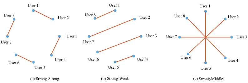
Figure 1: This figure illustrates pair selection in a typical cell of 8 users.

We study the influence of user pairing by considering three different user-pairing methods [44] and [45]. Fig. 1 illustrates pair selection in a typical cell of 8 users, where users are sorted in increasing order of channel gains, i.e., user 8 enjoys the strongest channel gain while user 1 is of the weakest channel gain. In strong-strong (SS) pair selection, the user with the strongest channel condition is paired with the one with the second strongest, and so on. In strong-weak (SW) pair selection, the user with the strongest channel condition is paired with the user with the weakest, and the user with the second strongest is paired with one with the second weakest, and so on. In strong-middle (SM) pair selection, the user with the strongest channel condition is paired with the user with the middle strongest user, i.e., user 8 is paired with user 4 in Fig. 1(c), and so on.

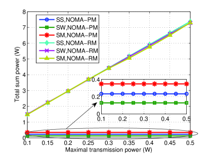
Figure 2: Sum power of the system for different user-pairing methods.

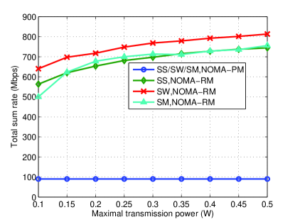
Figure 3: Sum rate of the system for different user-pairing methods.

In Fig. 2 and Fig. 3, we show the sum power and sum rate of the system for different user-pairing methods, respectively. From Fig. 2, it is observed that SW outperforms the other two methods in terms of power consumption for NOMA-PM. Besides, we can also find that SW achieves the best sum rate among three user-pairing methods for NOMA-RM according to Fig. 3. Combing Fig. 2 and Fig. 3, we can conclude that it tends to pair users with distinctive gains for both sum power minimization and sum rate maximization, which coincides with previous findings in [44]. Due to the superiority of SW, the following simulations are based on SW pair selection.

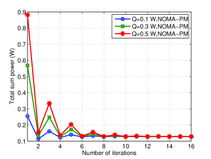
Figure 4: Convergence behavior of NOMA-PM.

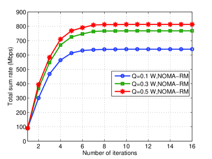
Figure 5: Convergence behavior of NOMA-RM.

The convergence behaviors of NOMA-PM and NOMA-RM are illustrated in Fig. 4 and Fig. 5, respectively. It can be seen that both NOMA-PM and NOMA-RM converge rapidly, which makes our proposed algorithms suitable for practical applications. From Fig. 5, the sum rate of NOMA-RM monotonically increases, which confirms the convergence analysis in Section IV-C.

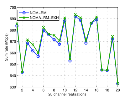
Figure 6: Performance comparison of NOMA-RM and NOMA-RM-EXH.

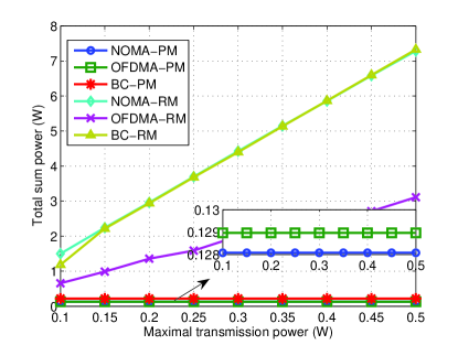
Figure 7: Sum power of the system versus the maximal transmission power.

We try multiple starting points in the simulations to exhaustively obtain a near globally optimal solution. We test 20 randomly generated channels shown in Fig. 6, where NOMA-RM-EXH refers to the NOMA-RM algorithm with 1000 starting points for each channel realization. It can be seen that the sum rate of NOMA-RM is almost the same as that of NOMA-RM-EXH, which indicates that the proposed NOMA-RM approaches the near globally optimal solution.

Fig. 7 shows the sum power versus the maximal transmission power under various algorithms. It is observed that the sum power of NOMA/OFDMA/BC-RM increases with the transmission power constraint. This is because increasing the overall transmission power is always beneficial in enhancing the sum rate of the system. It is also found that the sum power keeps the same for NOMA/OFDMA/BC-PM. This is due to that the maximal transmission power for each BS is set as the same and the sum power does not change value with the maximal transmission power for power minimization. From Fig. 7, the NOMA-PM is better than OFDMA/BC-PM in terms of the sum power consumption. The reason is that NOMA applies SIC to utilize intra-cell interference and each user can occupy the total available bandwidth, which results in lower sum power than OFDMA and BC.

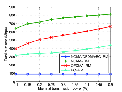
Figure 8: Sum rate of the system versus the maximal transmission power.

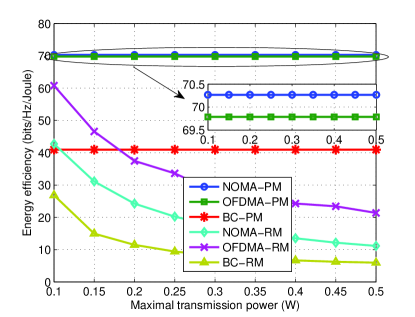
Figure 9: Energy efficiency of the system versus the maximal transmission power.

We illustrate the sum rate and energy efficiency (the ratio of sum rate and sum power) versus the maximal transmission power under various algorithms in Fig. 8 and Fig. 9, respectively. It is seen from Fig. 8 that the sum rate is the same for NOMA/OFDMA/BC-PM. Due to power minimization, each user is set as satisfying the minimal rate demand. Therefore, the sum rate of NOMA/OFDMA/BC-PM keeps a constant, i.e., $2IMR$, as shown in Fig. 8. From Fig. 8, it is observed that NOMA-RM outperforms OFDMA/BC-RM in terms of sum rate. One reason is that each user in NOMA networks can be allocated with higher fraction of bandwidth than in OFDMA networks, where the bandwidth is orthogonally distributed to different users in the same cell. The other reason is that NOMA can efficiently utilize intra-cell interference by using SIC, which results in higher rate than that of BC. From Fig. 9, it is interesting to observe that NOMA-PM achieves the best energy efficiency among all algorithms. It is also found that the energy efficiency of NOMA/OFDMA/BC-RM monotonically decreases with the maximal transmission power. This is because sum rate maximization algorithms tend to transmit with large power from Fig. 7, which results in large intra/inter-interference and low energy efficiency. NOMA needs to broadcast additional information about the decoding orders and the receivers at the users are complicated compared with OFDMA/BC-PM. Thus, we can conclude that NOMA achieves some performance gains at the cost of some additional information broadcasting of the BS and extra computations of the users from Fig. 7 and Fig. 8.

VII Conclusion

In this paper, we aim at sum power minimization and sum rate maximization through power control for multi-cell networks with NOMA. Both sum power minimization and sum rate maximization problems can be transformed into correspondingly equivalent problems with smaller variables. For sum power minimization, users with poor channel gains tend to be allocated with more power. Sum rate maximization problem can be decoupled into two subproblems, i.e., power allocation problem in a single cell and power control problem in multiple cells. The power allocation problem in a single cell is proved to be convex and its globally optimal solution can be obtained in the closed-form expression. Based on the optimal solution to power allocation problem in a single cell, only user in each cell with the best channel gain deserves additional power from its served BS to maximize sum rate in multi-cell networks with NOMA. Through simulation results, it tends to pair users with distinctive channel gains for both sum power minimization and sum rate maximization. It is shown that the proposed power control methods can be applied to MIMO systems. It is also verified that NOMA outperforms OFDMA and BC in terms of sum power minimization and sum rate maximization at the cost of some additional information broadcasting of the BSs and computations of the users. The users’ mobility issue for multi-cell NOMA systems is left for our future work.

Appendix A Proof of Theorem 1

To prove Theorem 1, we find that the objective function (9) is only a function of $\boldsymbol{q}$ and variable $\boldsymbol{p}$ only exists in constraints (8b), (8c) and $\boldsymbol{p}\geq\boldsymbol{0}$. Hence, $\boldsymbol{p}$ can be viewed as an intermediate variable. With this observation, sum power minimization Problem (8) with objective function (9) can be simplified by removing $\boldsymbol{p}$ without loss of optimality. Specifically, the constraints (8b), (8c) and $\boldsymbol{p}\geq\boldsymbol{0}$ about variable $\boldsymbol{p}$ can be equivalently transformed into constraints about $\boldsymbol{q}$.

Given total transmission power of other BSs, inter-cell interference is fixed, hence Problem (8) with objective function (9) can be readily simplified into a single-cell power allocation problem. For BS $i$, the power allocation problem with given $\boldsymbol{q}_{-i}=[q_{11},\cdots,q_{(i-1)M},q_{(i+1)1},\cdots,q_{IM}]^{T}$ can be formulated as

$$\mathop{\min}_{\boldsymbol{p}_{i}\geq\boldsymbol{0},\boldsymbol{q}_{i}\geq\boldsymbol{0}}\;\quad \sum_{m=1}^{M}q_{im}$$ (A.1a)

s.t. $$\sum_{j=J_{i(m-1)}+1}^{J_{im}}p_{ijm}=q_{im},\quad\forall m\in\mathcal{M}$$ (A.1b)

$$p_{ijm}\geq\left(2^{\frac{R_{ijm}}{B}}-1\right)\left(\sum_{n=j+1}^{J_{im}}p_{inm}+H_{ijm}\right),$$

$$\qquad\quad\forall m\in\mathcal{M},j\in\mathcal{J}_{im},$$ (A.1c)

where $\boldsymbol{p}_{i}=[p_{i(J_{i0}+1)1},\cdots,p_{iJ_{iM}M}]^{T}$, and $\boldsymbol{q}_{i}=[q_{i1},\cdots,q_{iM}]^{T}$.

Observing that both the objective function and constraints of Problem (A.1) can be decoupled, Problem (A.1) can be further decoupled into multiple single-subchannel problems. We consider the following optimization problem on subchannel $m$:

$$\mathop{\min}_{\boldsymbol{p}_{im}\geq\boldsymbol{0}}\;\quad \sum_{j=J_{i(m-1)}+1}^{J_{im}}p_{ijm}$$ (A.2a)

s.t. $$p_{ijm}\geq\left(2^{\frac{R_{ijm}}{B}}-1\right)\left(\sum_{n=j+1}^{J_{im}}p_{inm}+H_{ijm}\right),$$

$$\qquad\quad\forall j\in\mathcal{J}_{im},$$ (A.2b)

where $\boldsymbol{p}_{im}=[p_{i(J_{i(m-1)}+1)m},\cdots,p_{iJ_{im}m}]^{T}$. Combining (A.2b) and $\boldsymbol{p}_{im}\geq\boldsymbol{0}$, we find that constraints (A.2b) hold with equality for any optimal solution to Problem (A.2), as otherwise (A.2a) can be further improved, contradicting that the solution is optimal. Setting constraints (A.2b) with equality, we obtain

$$2^{\frac{R_{ijm}}{B}}\sum_{n=j+1}^{J_{im}}p_{inm}+\left(2^{\frac{R_{ijm}}{B}}-1\right)H_{ijm}=\sum_{n=j}^{J_{im}}p_{inm},$$ (A.3)

for all $j\in\mathcal{J}_{im}$. Define

$$b_{ijm}=\sum_{n=j}^{J_{im}}p_{inm},\quad j\in\mathcal{J}_{im},$$ (A.4)

which represents the summation of the transmission power from user $j$ to user $J_{im}$. Based on (A.3) and (A.4), we can obtain

$${b_{ijm}}={2^{\frac{R_{ijm}}{B}}}b_{i({j+1})m}+{\left(2^{\frac{R_{ijm}}{B}}-1\right)H_{ijm}},\quad\forall j\in\mathcal{J}_{i}.$$ (A.5)

Defining $b_{i(J_{im}+1)m}=0$ and ${2^{\sum_{s=J_{im}}^{J_{im}-1}\frac{R_{ism}}{B}}}=2^{0}$, we can rewrite (A.5) as follows:

$$b_{ijm}=\sum_{n=j}^{J_{im}}{\left(2^{\frac{R_{inm}}{B}}-1\right)}{2^{\sum_{s=j}^{n-1}\frac{R_{ism}}{B}}}H_{inm},\quad j\in\mathcal{J}_{im}.$$ (A.6)

According to (A.4), we know $p_{ijm}=b_{ijm}-b_{i(j+1)m},\forall j\in\mathcal{J}_{im}$. Substituting (A.6) into $p_{ijm}=b_{ijm}-b_{i(j+1)m}$ yields

$$p_{ijm} =\sum_{n=j}^{J_{im}}{\left(2^{\frac{R_{inm}}{B}}-1\right)}{2^{\sum_{s=j}^{n-1}\frac{R_{ism}}{B}}}H_{inm}-$$ (A.7)

$$\sum_{n=j+1}^{J_{im}}{\left(2^{\frac{R_{inm}}{B}}-1\right)}{2^{\sum_{s=j+1}^{n-1}\frac{R_{ism}}{B}}}H_{inm},\quad\forall j\in\mathcal{J}_{im},$$

which is the optimal solution to Problem (A.2).

From (A.4) and (A.6), the optimal objective value of Problem (A.2) is

$$q_{im} \!\!\!\!\!\!\!\!\!\!=\sum_{j=J_{i(m-1)}+1}^{J_{im}}p_{ijm}$$

$$\!\!\!\!\!\!\!\!\!\!=\sum_{n=J_{i(m-1)}+1}^{J_{im}}{\left(2^{\frac{R_{inm}}{B}}-1\right)}{2^{\sum_{s=J_{i(m-1)}+1}^{n-1}\frac{R_{ism}}{B}}}H_{inm},$$

which is minimal sum power of $\sum_{j=J_{i(m-1)}+1}^{J_{im}}p_{ijm}$ satisfying (A.2b) and $\boldsymbol{p}_{im}\geq\boldsymbol{0}$. Applying (A) into Problem (8) with objective function (9) yields equivalent Problem (11), where the inequality shown in (11b) is due to the fact that (A) is the minimal value of $q_{im}$.

Appendix B Proof of Theorem 2

We prove each of the three properties required for standard function below.

Positivity: Since $\max\limits_{l\in\{j,\cdots,J_{i}\}}\frac{\sigma^{2}}{|h_{ilm}|^{2}}>0$ for $j\in\mathcal{J}_{im}$, we have $f_{im}(\boldsymbol{q})>0$ from (11b).

Monotonicity: Let total transmission power vector $\boldsymbol{q}^{(1)}=[q_{11}^{(1)},\cdots,q_{IM}^{(1)}]^{T}$ and $\boldsymbol{q}^{(2)}=[q_{11}^{(2)},\cdots,q_{IM}^{(2)}]^{T}$ be such that $q_{im}^{(1)}\geq q_{im}^{(2)}$, $\forall i\in\mathcal{I},m\in\mathcal{M}$. Then, we have

$$\!\!\!\!\!\!\!\!\!\!\max_{l\in\{j,\cdots,J_{i}\}}\frac{\sum_{k\in\mathcal{I}\setminus\{i\}}q_{km}^{(1)}|h_{klm}|^{2}+\sigma^{2}}{|h_{ilm}|^{2}}$$

$$\!\!\!\!\!\!\!\!\!\!\geq\max_{l\in\{j,\cdots,J_{im}\}}\frac{\sum_{k\in\mathcal{I}\setminus\{i\}}q_{km}^{(2)}|h_{klm}|^{2}+\sigma^{2}}{|h_{ilm}|^{2}}.$$ (B.1)

According to (B) and (11b), we have $f_{im}(\boldsymbol{q}^{(1)})\geq f_{im}(\boldsymbol{q}^{(2)})$.

Scalability: Letting $\boldsymbol{q}\geq\boldsymbol{0}$ and $\lambda>1$, we have

$$\!\!\!\!\!\!\!\!\!\!\max_{l\in\{j,\cdots,J_{im}\}}\lambda\frac{\sum_{k\in\mathcal{I}\setminus\{i\}}q_{km}|h_{klm}|^{2}+\sigma^{2}}{|h_{ilm}|^{2}}$$

$$\!\!\!\!\!\!\!\!\!\!>\max_{l\in\{j,\cdots,J_{im}\}}\frac{\sum_{k\in\mathcal{I}\setminus\{i\}}\lambda q_{km}|h_{klm}|^{2}+\sigma^{2}}{|h_{ilm}|^{2}},$$ (B.2)

where the inequality follows from that $\sigma^{2}>0$. Based on (B) and (11b), we have $\lambda f_{im}(\boldsymbol{q})>f_{im}(\lambda\boldsymbol{q})$.

Appendix C Proof of Theorem 3

Since the constraints of Problem (15) are all linear, we only need to prove that the objective function (15a) is convex. We first rewrite (15a) as

$$R_{im}= \!\!\!\!\!\!\!\!\!-B\log_{2}\left({\sum_{n=J_{i(m-1)}+1}^{J_{im}}p_{inm}+H_{i(J_{i(m-1)}+1)m}}\right)$$

$$\!\!\!\!\!\!\!\!\!+\sum_{j=J_{i(m-1)}+2}^{J_{im}}B\left(\log_{2}\left({\sum_{n=j}^{J_{im}}p_{inm}+H_{i(j-1)m}}\right)\right.$$

$$\!\!\!\!\!\!\!\!\!\!\left.-\log_{2}\left({\sum_{n=j}^{J_{im}}p_{inm}+H_{ijm}}\right)\right)+B\log_{2}(H_{iJ_{im}m}),$$

where $R_{im}$ is negative sum rate of all users served by BS $i$ on subchannel $m$. The second-order derivative of $R_{im}$ equals

$$\!\!\!\!\!\!\!\!\!\frac{\partial^{2}R_{im}}{\partial p_{ijm}^{2}}=\sum_{l=J_{i(m-1)}+2}^{j}\frac{1}{\ln 2}\left(\frac{B}{\left({\sum_{n=l}^{J_{im}}p_{inm}+H_{ijm}}\right)^{2}}\right.$$

$$\!\!\!\!\!\!\!\!\!\!\!\left.-\frac{B}{\left({\sum_{n=l}^{J_{im}}p_{inm}+H_{i(j-1)m}}\right)^{2}}\right)$$

$$\!\!\!\!\!\!\!\!\!\!\!+\frac{B}{(\ln 2)\left(\sum_{n=J_{i(m-1)}+1}^{J_{im}}p_{inm}+H_{i(J_{i(m-1)}+1)m}\right)^{2}}$$ (C.1)

for all $j=J_{i-1}+1,J_{i-1}+2,\cdots,J_{i}$, and

$$\!\!\!\!\!\!\!\!\!\frac{\partial^{2}R}{\partial p_{ijm}\partial p_{ilm}}=\sum_{l=J_{i(m-1)}+2}^{j}\frac{1}{\ln 2}\left(\frac{B}{\left({\sum_{n=l}^{J_{im}}p_{inm}+H_{ijm}}\right)^{2}}\right.$$

$$\!\!\!\!\!\!\!\!\!\!\!\left.-\frac{B}{\left({\sum_{n=l}^{J_{im}}p_{inm}+H_{i(j-1)m}}\right)^{2}}\right)$$

$$\!\!\!\!\!\!\!\!\!\!\!+\frac{B}{(\ln 2)\left(\sum_{n=J_{i(m-1)}+1}^{J_{im}}p_{inm}+H_{i(J_{i(m-1)}+1)m}\right)^{2}}$$ (C.2)

for all $J_{i-1}+\leq j<l\leq J_{i}$. Comparing (C.1) and (C.2), we find that $\frac{\partial^{2}R_{im}}{\partial p_{ijm}\partial p_{ilm}}=\frac{\partial^{2}R_{im}}{\partial p_{ijm}^{2}}$ for any $J_{i(m-1)}+1\leq j\leq l\leq J_{im}$. Therefore, denoting $a_{ijm}=\frac{\partial^{2}R_{im}}{\partial p_{ijm}^{2}}$ for notational simplicity, the Hessian matrix $\boldsymbol{A}_{im}$ of (15a) has the following structure:

$$\boldsymbol{A}_{im}\!\!=\!\!\!\begin{pmatrix}\!a_{i(J_{i(m-1)}+1)m}\!&\!\!\!a_{i(J_{i(m-1)}+1)m}\!\!\!&\!\cdots\!&\!\!\!a_{i(J_{i(m-1)}+1)m}\!\\ \!a_{i(J_{i(m-1)}+1)m}\!&\!\!\!a_{i(J_{i(m-1)}+2)m}\!\!\!&\!\cdots\!&\!\!\!a_{i(J_{i(m-1)}+2)m}\!\\ \vdots&\vdots\ &&\vdots\\ \!a_{i(J_{i(m-1)}+1)m}\!&\!\!\!a_{i(J_{i(m-1)}+2)m}\!\!\!&\!\cdots\!&\!\!\!a_{iJ_{im}m}\!\end{pmatrix}\!\!.$$ (C.3)

Based on (C.3), the $t$-th order principal minor of matrix $\boldsymbol{A}_{im}$ can be expressed as

$$A_{imt}\!\! \!\!\!\!\!\!\!\!\!=\!\begin{vmatrix}\!a_{i(J_{i(m-1)}+1)m}\!\!&\!\!a_{i(J_{i(m-1)}+1)m}\!\!&\!\cdots\!&\!\!a_{i(J_{i(m-1)}+1)m}\!\\ \!a_{i(J_{i(m-1)}+1)m}\!\!&\!\!a_{i(J_{i(m-1)}+2)m}\!\!&\!\cdots\!&\!\!a_{i(J_{i(m-1)}+2)m}\!\\ \vdots&\vdots&&\vdots\\ \!a_{i(J_{i(m-1)}+1)m}\!\!&\!\!a_{i(J_{i(m-1)}+2)m}\!\!&\!\cdots\!&\!\!a_{i(J_{i(m-1)}+t)m}\!\\ \end{vmatrix}$$

$$\!\!\!\!\!\!\!\!\!\!\!=a_{i(J_{i(m-1)}+1)m}\prod_{l=2}^{t}(a_{i(J_{i(m-1)}+l)m}-a_{i(J_{i(m-1)}+l-1)m}).$$

Since

$$a_{i(J_{i(m-1)}+1)m} \!\!\!\!\!\!\!\!\!\!=\!\frac{B/(\ln 2)}{\left(\sum_{n=J_{i(m-1)}+1}^{J_{im}}p_{inm}+H_{i(J_{i(m-1)}+1)m}\right)^{2}}$$

$$\!\!\!\!\!\!\!\!\!\!>0,$$

and for $J_{i(m-1)}+2\leq l\leq J_{im}$,

$$\!\!\!\!\!\!\!\!\!\!\!\!\!\!\!\!\!\quad a_{i(J_{i(m-1)}+l)m}-a_{i(J_{i(m-1)}+l-1)m}$$

$$\!\!\!\!\!\!\!\!\!\!\!\!\!\!\!\!\!\quad=\frac{1}{\ln 2}\left(\frac{B}{\left({\sum_{n=J_{i(m-1)}+l}^{J_{im}}p_{inm}+H_{i(J_{i(m-1)}+l)m}}\right)^{2}}\right.$$

$$\!\!\!\!\!\!\!\!\!\!\!\!\!\!\!\!\!\qquad\left.-\frac{B}{\left({\sum_{n=J_{i(m-1)}+l}^{J_{im}}p_{inm}+H_{i(J_{i(m-1)}+l-1)m}}\right)^{2}}\right)\overset{(\text{a})}{\geq}0,$$

where inequality (a) holds based on (III-C), we have from (LABEL:hessianT) that $A_{imt}\geq 0$ for $t=1,\cdots,J_{im}-J_{i(m-1)}$. According to [46, Page 558], a function whose Hessian is positive semi-definite throughout a convex set is convex. Besides, if the principal minors of a matrix are all nonnegative, this matrix is positive semi-definite [46, Page 558]. Thus, matrix $\boldsymbol{A}_{im}$ is positive semi-definite, which implies that objective function (15a) is convex. As a result, Problem (15) is convex.

Then, we prove the feasibility condition for Problem (15). To prove this, we denote

$$\tilde{q}_{im}=\left\{\begin{array}[]{ll}\!\!\mathop{\min}\limits_{\boldsymbol{p}_{im}\geq\boldsymbol{0}}&\!\sum_{j=J_{i(m-1)}+1}^{J_{im}}p_{ijm}\\ \>\textrm{s.t.}&\!p_{ijm}\!\geq\!\!\left(\!2^{\frac{R_{ijm}}{B}}\!-\!1\!\right)\!\left(\!\sum_{n=j+1}^{J_{im}}\!p_{inm}\!+\!H_{ijm}\!\right),\\ &\qquad\forall j\in\mathcal{J}_{im}.\end{array}\right.$$

From (15b), (15c), and $\boldsymbol{p}_{im}\geq\boldsymbol{0}$, we can find that Problem (15) is feasible if and only if $\tilde{q}_{im}\leq q_{im}$. To obtain $\tilde{q}_{im}$, we observe that constraints (15c) hold with equality for all $j\in\mathcal{J}_{im}$, as otherwise $\tilde{q}_{im}$ can be further improved. By solving these $J_{im}-J_{i(m-1)}$ linear equations, we have $\tilde{q}_{im}=\sum_{n=J_{i(m-1)}+1}^{J_{im}}{\left(2^{\frac{R_{inm}}{B}}-1\right)}{2^{\sum_{s=J_{i(m-1)}+1}^{n-1}\frac{R_{ism}}{B}}}H_{inm}$ from (A.3), (A.4) and (A). Hence, the feasibility condition for Problem (15) is achieved as (16).

Appendix D Proof of Theorem 4

The Lagrangian function of Problem (15) can be written by

$$\!\!\!\!\!\!\!\!\mathcal{L}(\boldsymbol{p}_{im},\alpha_{im},\boldsymbol{\beta}_{im},\boldsymbol{\gamma}_{im})=\alpha_{im}\!\left(\!\sum_{j=J_{i(m-1)}+1}^{J_{im}}p_{ijm}-q_{im}\right)$$

$$\!\!\!\!\!\!\!\!-\sum_{j=J_{i(m-1)}+1}^{J_{im}}B\log_{2}\left(1+\frac{p_{ijm}}{\sum_{n=j+1}^{J_{im}}p_{inm}+H_{ijm}}\right)$$

$$\!\!\!\!\!\!\!\!+\sum_{j=J_{i(m-1)}+1}^{J_{im}}\beta_{ijm}\left(\left(2^{\frac{R_{ijm}}{B}}-1\right)\left(\sum_{n=j+1}^{J_{im}}p_{inm}+H_{ijm}\right)\right.$$

$$\!\!\!\!\!\!\!\!-p_{ijm}\Bigg{)}-\sum_{j=J_{i(m-1)}+1}^{J_{im}}\gamma_{ijm}p_{ijm},$$

where $\alpha_{im}$, $\boldsymbol{\beta}_{im}=[\beta_{i(J_{i(m-1)}+1)m},\cdots,\beta_{iJ_{im}m}]^{T}\geq\boldsymbol{0}$ and $\boldsymbol{\gamma}_{im}=[\gamma_{i(J_{i(m-1)}+1)m},\cdots,\gamma_{iJ_{im}m}]^{T}\geq\boldsymbol{0}$ are the Lagrange multipliers associated with the corresponding constraints of Problem (15). The KKT conditions of Problem (15) are:

$$\frac{\partial\mathcal{L}}{\partial p_{ijm}}=-\frac{B}{(\ln 2)\left(\sum_{n=J_{i(m-1)}+1}^{J_{im}}p_{inm}+H_{i(J_{i(m-1)}+1)m}\right)}$$

$$\qquad+\alpha_{im}+\sum_{n=J_{i(m-1)}+1}^{j-1}\left(2^{\frac{R_{inm}}{B}}-1\right)\beta_{inm}-\beta_{ijm}$$

$$\qquad-\gamma_{ijm}-\sum_{l=J_{i(m-1)}+2}^{j}\frac{1}{\ln 2}\left(\frac{B}{{\sum_{n=l}^{J_{im}}p_{inm}+H_{ijm}}}\right.$$

$$\qquad\left.-\frac{B}{{\sum_{n=l}^{J_{im}}p_{inm}+H_{i(j-1)m}}}\right),\quad\forall j\in\mathcal{J}_{im}$$ (D.1a)

$$\beta_{ijm}\left(\left(2^{\frac{R_{ijm}}{B}}-1\right)\left(\sum_{n=j+1}^{J_{im}}p_{inm}+H_{ijm}\right)-p_{ijm}\right)=0,$$

$$\qquad\quad\forall j\in\mathcal{J}_{im}$$ (D.1b)

$$\gamma_{ijm}p_{ijm}=0,\quad\forall j\in\mathcal{J}_{im}$$ (D.1c)

$$\sum_{j=J_{i(m-1)}+1}^{J_{im}}p_{ijm}-q_{im}=0$$ (D.1d)

$$\left(2^{\frac{R_{ijm}}{B}}-1\right)\left(\sum_{n=j+1}^{J_{im}}p_{inm}+H_{ijm}\right)-p_{ijm}\leq 0,$$

$$\qquad\forall j\in\mathcal{J}_{im}$$ (D.1e)

$$\boldsymbol{\beta}_{im},\boldsymbol{\gamma}_{im},\boldsymbol{p}_{im}\geq\boldsymbol{0}.$$ (D.1f)

According to (D.1e) and $R_{ijm}>0$, we can obtain $p_{ijm}>0$, $\forall j\in\mathcal{J}_{im}$. Hence, further combing (D.1c), we have

$$\gamma_{ijm}=0,\quad\forall j\in\mathcal{J}_{im}.$$ (D.2)

Assume that

$${H_{i(J_{i(m-1)}+1)m}}>{H_{i(J_{i(m-1)}+2)m}}>\cdots>{H_{iJ_{im}m}}.$$ (D.3)

The special case with ${H_{i(j-1)m}}={H_{ijm}}$ for at least one $j\in\{J_{i(m-1)}+2,\cdots,J_{im}\}$ is considered later. From (D.1a) and (D.2), we obtain

$$\frac{\partial\mathcal{L}}{\partial p_{ijm}}-\frac{\partial\mathcal{L}}{\partial p_{i(j-1)m}} \!\!\!\!\!\!\!\!\!=\frac{1}{\ln 2}\left(\frac{B}{{\sum_{n=j}^{J_{im}}p_{inm}+H_{i(j-1)m}}}\right.$$

$$\!\!\!\!\!\!\!\!\!\!\!\left.-\frac{B}{{\sum_{n=j}^{J_{im}}p_{inm}+H_{ijm}}}\right)$$

$$\!\!\!\!\!\!\!\!\!\!\!-\beta_{ijm}+\beta_{i(j-1)m}2^{\frac{R_{i(j-1)m}}{B}}=0$$

for $j=J_{i(m-1)}+2,\cdots,J_{im}$. Considering (D.3), we have

$$\!\!\!\!\!\!\!\!\!\beta_{ijm}-\beta_{i(j-1)m}2^{\frac{R_{i(j-1)m}}{B}}$$

$$\!\!\!\!\!\!\!\!\!\!=\!\frac{1}{\ln 2}\!\left(\!\frac{B}{{\sum_{n=j}^{J_{im}}p_{inm}\!+\!{H_{i(j-1)m}}}}\!-\!\frac{B}{\!{\sum_{n=j}^{J_{im}}p_{inm}\!+\!{H_{ijm}}}}\right)<0$$

for $j=J_{i(m-1)}+2,\cdots,J_{im}$. Since $\beta_{ijm}\geq 0$, we have $\beta_{i(j-1)m}2^{\frac{R_{i(j-1)m}}{B}}>\beta_{ijm}\geq 0$, $j=J_{i(m-1)}+2,\cdots,J_{im}$. Thus, we can obtain $\beta_{i(J_{im}-1)m}>0$, $\cdots$, $\beta_{i(J_{i(m-1)}+1)m}>0$. Hence, we only need to consider the following two cases of $\beta_{iJ_{im}m}$ for user $J_{im}$.

1) If $\beta_{iJ_{im}m}>0$, constraints in (D.1b) are satisfied via $\left(2^{\frac{R_{ijm}}{B}}-1\right)\left(\sum_{n=j+1}^{J_{im}}p_{inm}+H_{ijm}\right)-p_{ijm}=0$ for all $j\in\mathcal{J}_{im}$, which implies that the minimal rate constraints (D.1e) hold with equality for all users. Thus, the optimal value of Problem (15) is $-\sum_{j=J_{i(m-1)}+1}^{J_{im}}R_{ijm}$, and the optimal solution to Problem (15) can be obtained as in (10) by solving constraints (D.1e) with equality for all users.

2) If $\beta_{iJ_{im}m}=0$, we find that constraints (D.1e) hold with equality except for the user $J_{im}$.

Due to that Problem (15) can be easily solved for the case $\beta_{iJ_{im}m}>0$, we only need to consider the case $\beta_{iJ_{im}m}=0$ in the following. Since minimal rate constraints (D.1e) hold with equality for $j\in\mathcal{J}_{im}\setminus\{J_{im}\}$, we find that the additional power is allocated to the user with the highest channel gain and other users served by BS $i$ on subchannel $m$ are allocated with minimal transmission power to meet the minimal rate demands. Now, it remains optimal to solve constraints (D.1e) with equality for $j\in\mathcal{J}_{im}\setminus\{J_{im}\}$. Thus, we have

$$2^{\frac{R_{ijm}}{B}}\sum_{n=j+1}^{J_{im}}p_{inm}+\left(2^{\frac{R_{ijm}}{B}}-1\right)H_{ijm}=\sum_{n=j}^{J_{im}}p_{inm},$$ (D.4)

for all $j=J_{i(m-1)}+1,\cdots,J_{im}-1$. Define

$$b_{ijm}=\sum_{n=j}^{J_{im}}p_{ijm},\quad j=J_{i(m-1)}+1,\cdots,J_{im}.$$ (D.5)

Substituting (D.5) into (D.1d) yields

$$b_{i(J_{i(m-1)}+1)}=q_{im}.$$ (D.6)

Based on (D.4) and (D.5), we can obtain

$$b_{i({j+1})m}=\frac{b_{ijm}}{2^{\frac{R_{ijm}}{B}}}-\frac{\left(2^{\frac{R_{ijm}}{B}}-1\right)H_{ij}}{2^{\frac{R_{ijm}}{B}}},$$ (D.7)

for all $j=J_{i(m-1)}+1,\cdots,J_{im}-1$. By further using (D.6), we have

$$b_{i(j+1)m}= \!\!\!\!\!\!\!\!\frac{q_{im}}{2^{\sum_{n=J_{i(m-1)}+1}^{j}\frac{R_{inm}}{B}}}$$ (D.8)

$$\!\!\!\!\!\!\!\!-\sum_{n=J_{i(m-1)}+1}^{j}\frac{\left(2^{\frac{R_{inm}}{B}}-1\right)H_{inm}}{2^{\sum_{l=n}^{j}\frac{R_{ilm}}{B}}},$$

for all $j=J_{i(m-1)}+1,\cdots,J_{im}-1$. From (D.5), we can obtain

$$p_{ijm}\!=\!\begin{cases}b_{ijm}-b_{i(j+1)m},&\!\!\!\!\!\mbox{ if $j=J_{i(m-1)}+1,\cdots,J_{im}-1$}\\ b_{ijm},&\!\!\!\!\!\mbox{ if $j=J_{im}$}\end{cases}.$$ (D.9)

By inserting (D.8) into (D.9), we can obtain closed-form expression of $p_{ijm}$ as (17). Substituting (17) into objective function (15a), we can obtain the optimal sum rate of Problem (15) as (18).

Now, we consider the special case remained to be discussed. Assume that there are two users served by BS $i$ with satisfying ${H_{i(j-1)m}}={H_{ijm}}$. In this case, we can define a new user $j^{\prime}$ with $R_{ij^{\prime}m}=R_{i(j-1)m}+R_{ijm}$. Calculate the optimal power allocation strategy $[p_{i(J_{i(m-1)}+1)m}^{*},\cdots,$ $p_{i(j-2)m}^{*},p_{ij^{\prime}m}^{*},p_{i(j+1)m}^{*},\cdots,p_{iJ_{im}m}^{*}]^{T}$ for users $J_{i(m-1)}+1,\cdots,j-2,j^{\prime},j+1,\cdots,J_{im}$ according to (17). Based on (5), we have

$$r_{i(j-1)m}+r_{ijm} \!\!\!\!\!\!\!\!\!\!=B\log_{2}\left(\frac{\sum_{n=j-1}^{J_{im}}p_{inm}\!+\!{H_{i(j-1)m}}}{\sum_{n=j}^{J_{im}}p_{inm}\!+\!{H_{i(j-1)m}}}\right)$$

$$\!\!\!\!\!\!\!\!\!\!\quad+B\log_{2}\left(\frac{\sum_{n=j}^{J_{im}}p_{inm}\!+\!{H_{ijm}}}{\sum_{n=j+1}^{J_{im}}p_{inm}\!+\!{H_{ijm}}}\right)$$

$$\!\!\!\!\!\!\!\!\!\!=B\log_{2}\left(\frac{\sum_{n=j-1}^{J_{im}}p_{inm}+{H_{ijm}}}{\sum_{n=j+1}^{J_{im}}p_{inm}+{H_{ijm}}}\right),$$

which means that the sum rate of user $j-1$ and user $j$ is determined by the sum power $p_{i(j-1)m}+p_{ijm}$. In the optimal power allocation strategy for user $j-1$ and user $j$, we can arbitrarily allocate power $p_{i(j-1)m}^{*}$ and $p_{ijm}^{*}$ with $p_{i(j-1)m}^{*}+p_{ijm}^{*}=p_{ij^{\prime}m}^{*}$ fixed and the minimal rate constraints $r_{i(j-1)m}^{*}\geq R_{i(j-1)m}$ and $r_{ijm}^{*}\geq R_{ijm}$ satisfied. If $j\neq J_{im}$, we can observe that $r_{ij^{\prime}m}^{*}=R_{ij^{\prime}m}=R_{i(j-1)m}+R_{ijm}$ according to (D.4) for the optimal power allocation strategy. Then, $r_{i(j-1)m}^{*}=R_{i(j-1)m}$ and $r_{ijm}^{*}=R_{ijm}$, which indicates that the optimal power for user $j-1$ and user $j$ can be presented as (17). If $j=J_{im}$, we can observe that $r_{ij^{\prime}m}^{*}\geq R_{ij^{\prime}m}$ according to (D.1e) for the optimal power allocation strategy. If we set $r_{i(j-1)m}^{*}=R_{i(j-1)m}$ and $r_{ijm}^{*}=r_{ij^{\prime}m}^{*}-R_{ijm}$, the optimal power for user $j-1$ and user $j$ can also be presented as (17). Thus, we can still obtain the optimal sum rate of Problem (15) as (18).

As a result, Theorem 4 is proved.

References

• [1] J. Thompson, X. Ge, H.-C. Wu, R. Irmer, H. Jiang, G. Fettweis, and S. Alamouti, “5G wireless communication systems: Prospects and challenges,” IEEE Commun. Mag., vol. 52, no. 2, pp. 62–64, Feb. 2014.
• [2] L. Dai, B. Wang, Y. Yuan, S. Han, C. l. I, and Z. Wang, “Non-orthogonal multiple access for 5G: Solutions, challenges, opportunities, and future research trends,” IEEE Commun. Mag., vol. 53, no. 9, pp. 74–81, Sep. 2015.
• [3] Z. Ding, X. Lei, G. K. Karagiannidis, R. Schober, J. Yuan, and V. K. Bhargava, “A survey on non-orthogonal multiple access for 5G networks: Research challenges and future trends,” IEEE J. Sel. Areas Commun., vol. 35, no. 10, pp. 2181–2195, Oct. 2017.
• [4] A. Bayesteh, E. Yi, H. Nikopour, and H. Baligh, “Blind detection of SCMA for uplink grant-free multiple-access,” in Proc. Int. Symp. Wireless Commun. Syst. (ISWCS), Aug. 2014, pp. 853–857.
• [5] B. Wang, L. Dai, T. Mir, and Z. Wang, “Joint user activity and data detection based on structured compressive sensing for NOMA,” IEEE Commun. Lett., vol. 20, no. 7, pp. 1473–1476, Jul. 2016.
• [6] B. Wang, L. Dai, Y. Zhang, T. Mir, and J. Li, “Dynamic compressive sensing-based multi-user detection for uplink grant-free NOMA,” IEEE Commun. Lett., vol. 20, no. 11, pp. 2320–2323, Nov. 2016.
• [7] C. Wei, H. Liu, Z. Zhang, J. Dang, and L. Wu, “Approximate message passing based joint user activity and data detection for NOMA,” IEEE Commun. Lett., vol. PP, no. 99, pp. 1–1, Dec. 2016.
• [8] Y. Saito, Y. Kishiyama, A. Benjebbour, T. Nakamura, A. Li, and K. Higuchi, “Non-orthogonal multiple access (NOMA) for cellular future radio access,” in Proc. IEEE Veh. Technol. Conf.   Dresden, German, Jun. 2013, pp. 1–5.
• [9] Z. Ding, Y. Liu, J. Choi, Q. Sun, M. Elkashlan, and H. V. Poor, “Application of non-orthogonal multiple access in LTE and 5G networks,” IEEE Commun. Mag., vol. 55, no. 2, pp. 185–191, Feb. 2017.
• [10] Z. Ding, F. Adachi, and H. V. Poor, “The application of MIMO to non-orthogonal multiple access,” IEEE Trans. Wireless Commun., vol. 15, no. 1, pp. 537–552, Jan. 2016.
• [11] S. M. R. Islam, N. Avazov, O. A. Dobre, and K. S. Kwak, “Power-domain non-orthogonal multiple access (NOMA) in 5G systems: Potentials and challenges,” IEEE Commun. Surveys Tutorials, vol. PP, no. 99, pp. 1–1, Oct. 2016.
• [12] Y. Saito, A. Benjebbour, Y. Kishiyama, and T. Nakamura, “System-level performance evaluation of downlink non-orthogonal multiple access (NOMA),” in Proc. IEEE Annu. Symp. Personal, Indoor and Mobile Radio Commun.   London, U.K., Sept. 2013, pp. 611–615.
• [13] Z. Ding, Z. Yang, P. Fan, and H. V. Poor, “On the performance of non-orthogonal multiple access in 5G systems with randomly deployed users,” IEEE Signal Process. Lett., vol. 21, no. 12, pp. 1501–1505, Jul. 2014.
• [14] A. Benjebbovu, A. Li, Y. Saito, Y. Kishiyama, A. Harada, and T. Nakamura, “System-level performance of downlink NOMA for future LTE enhancements,” in Proc. IEEE Globecom Workshops, Dec. 2013, pp. 66–70.
• [15] M. F. Hanif, Z. Ding, T. Ratnarajah, and G. K. Karagiannidis, “A minorization-maximization method for optimizing sum rate in the downlink of non-orthogonal multiple access systems,” IEEE Trans. Signal Process., vol. 64, no. 1, pp. 76–88, Jan. 2016.
• [16] Z. Yang, W. Xu, C. Pan, Y. Pan, and M. Chen, “On the optimality of power allocation for NOMA downlinks with individual QoS constraints,” IEEE Commun. Lett., vol. PP, no. 99, pp. 1–1, 2017.
• [17] S. Timotheou and I. Krikidis, “Fairness for non-orthogonal multiple access in 5G systems,” IEEE Signal Process. Lett., vol. 22, no. 10, pp. 1647–1651, Oct. 2015.
• [18] X. Chen, A. Benjebbour, A. Li, and A. Harada, “Multi-user proportional fair scheduling for uplink non-orthogonal multiple access (NOMA),” in Proc. IEEE Veh. Technol. Conf.   Seoul, Korea, May 2014, pp. 1–5.
• [19] Z. Yang, W. Xu, and Y. Li, “Fair non-orthogonal multiple access for visible light communication downlinks,” IEEE Wireless Commun. Lett., vol. 6, no. 1, pp. 66–69, Feb. 2017.
• [20] Y. Zhang, H. M. Wang, T. X. Zheng, and Q. Yang, “Energy-efficient transmission design in non-orthogonal multiple access,” IEEE Trans. Veh. Technol., vol. 66, no. 3, Mar. 2017.
• [21] Z. Yang, W. Xu, H. Xu, J. Shi, and M. Chen, “Energy efficient non-orthogonal multiple access for machine-to-machine communications,” IEEE Commun. Lett., vol. 21, no. 4, pp. 817–820, Apr. 2017.
• [22] L. Lei, D. Yuan, C. K. Ho, and S. Sun, “Power and channel allocation for non-orthogonal multiple access in 5G systems: Tractability and computation,” IEEE Trans. Wireless Commun., vol. 15, no. 12, pp. 8580–8594, Dec. 2016.
• [23] P. Parida and S. S. Das, “Power allocation in OFDM based NOMA systems: A DC programming approach,” in Proc. IEEE Globecom Workshops, Dec. 2014, pp. 1026–1031.
• [24] F. Fang, H. Zhang, J. Cheng, and V. C. M. Leung, “Energy-efficient resource allocation for downlink non-orthogonal multiple access network,” IEEE Trans. Commun., vol. 64, no. 9, pp. 3722–3732, Sep. 2016.
• [25] B. Di, L. Song, and Y. Li, “Sub-channel assignment, power allocation, and user scheduling for non-orthogonal multiple access networks,” IEEE Trans. Wireless Commun., vol. 15, no. 11, pp. 7686–7698, Nov. 2016.
• [26] L. Lei, D. Yuan, and P. Värbrand, “On power minimization for non-orthogonal multiple access (NOMA),” IEEE Commun. Lett., vol. 20, no. 12, pp. 2458–2461, Dec. 2016.
• [27] J. Choi, “Non-orthogonal multiple access in downlink coordinated two-point systems,” IEEE Commun. Lett., vol. 18, no. 2, pp. 313–316, Feb. 2014.
• [28] W. Shin, M. Vaezi, B. Lee, D. J. Love, J. Lee, and H. V. Poor, “Coordinated beamforming for multi-cell MIMO-NOMA,” IEEE Commun. Lett., vol. 21, no. 1, pp. 84–87, Jan. 2017.
• [29] ——, “Non-orthogonal multiple access in multi-cell networks: Theory, performance, and practical challenges,” IEEE Commun. Mag., vol. PP, no. 99, pp. 2–9, 2017.
• [30] S. Han, I. Chih-Lin, Z. Xu, and Q. Sun, “Energy efficiency and spectrum efficiency co-design: From NOMA to network NOMA,” E-Lett., 2014.
• [31] C. W. Sung and Y. Fu, “A game-theoretic analysis of uplink power control for a non-orthogonal multiple access system with two interfering cells,” in Proc. IEEE Veh. Technol. Conf., May 2016, pp. 1–5.
• [32] Y. Fu, Y. Chen, and C. W. Sung, “Distributed downlink power control for the non-orthogonal multiple access system with two interfering cells,” in Proc. IEEE Int. Conf. Commun., May. 2016, pp. 1–6.
• [33] V. D. Nguyen, H. D. Tuan, T. Q. Duong, H. V. Poor, and O. S. Shin, “Precoder design for signal superposition in MIMO-NOMA multicell networks,” IEEE J. Sel. Areas Commun., vol. PP, no. 99, pp. 1–1, 2017.
• [34] D. Lee, H. Seo, B. Clerckx, E. Hardouin, D. Mazzarese, S. Nagata, and K. Sayana, “Coordinated multipoint transmission and reception in LTE-advanced: Deployment scenarios and operational challenges,” IEEE Commun. Mag., vol. 50, no. 2, pp. 148–155, Feb. 2012.
• [35] R. D. Yates, “A framework for uplink power control in cellular radio systems,” IEEE J. Sel. Areas Commun., vol. 13, no. 7, pp. 1341–1347, Sep. 1995.
• [36] S. Boyd and L. Vandenberghe, Convex Optimization.   Cambridge University Press, 2004.
• [37] D. P. Bertsekas, Convex Optimization Theory.   Athena Scientific Belmont, 2009.
• [38] N. Vucic, S. Shi, and M. Schubert, “DC programming approach for resource allocation in wireless networks,” in Proc. Int. Symp. Modeling Optim. Mobile, Ad Hoc Wireless Netw., May 2010, pp. 380–386.
• [39] C. K. Ho, D. Yuan, L. Lei, and S. Sun, “Power and load coupling in cellular networks for energy optimization,” IEEE Trans. Wireless Commun., vol. 14, no. 1, pp. 509–519, Jan. 2015.
• [40] Access, Evolved Universal Terrestrial Radio, “Further advancements for E-UTRA physical layer aspects, 3GPP TS 36.814,” V9. 0.0, Mar., 2010.
• [41] A. Zafar, M. Shaqfeh, M. S. Alouini, and H. Alnuweiri, “On multiple users scheduling using superposition coding over rayleigh fading channels,” IEEE Commun. Lett., vol. 17, no. 4, pp. 733–736, Apr. 2013.
• [42] Z. Yang, C. Pan, W. Xu, H. Xu, and M. Chen, “Joint time allocation and power control in multi-cell networks with load coupling: Energy saving and rate improvement,” IEEE Trans. Veh. Technol., vol. PP, no. 99, pp. 1–1, 2017.
• [43] Q. Shi, M. Razaviyayn, Z. Q. Luo, and C. He, “An iteratively weighted MMSE approach to distributed sum-utility maximization for a MIMO interfering broadcast channel,” IEEE Trans. Signal Process., vol. 59, no. 9, pp. 4331–4340, Sep. 2011.
• [44] Z. Ding, P. Fan, and H. V. Poor, “Impact of user pairing on 5G nonorthogonal multiple-access downlink transmissions,” IEEE Trans. Veh. Technol., vol. 65, no. 8, pp. 6010–6023, Aug. 2016.
• [45] L. You, D. Yuan, L. Lei, S. Sun, S. Chatzinotas, and B. Ottersten, “Resource optimization in multi-cell NOMA,” 2017. [Online]. Available: https://arxiv.org/abs/1708.05281
• [46] R. A. Horn and C. R. Johnson, Matrix Analysis.   Cambridge University Press, 2012.