A Dust Twin of Cas A:
Cool Dust and 21$\mu$m Silicate Dust Feature in the Supernova Remnant G54.1+0.3

Abstract

We present infrared (IR) and submillimeter observations of the Crab-like supernova remnant (SNR) G54.1+0.3 including 350$\mu$m (SHARC-II), 870$\mu$m (LABOCA), 70, 100, 160, 250, 350, 500$\mu$m (Herschel) and 3-40$\mu$m (Spitzer). We detect dust features at 9, 11 and 21$\mu$m and a long wavelength continuum dust component. The 21$\mu$m dust coincides with [Ar II] ejecta emission, and the feature is remarkably similar to that in Cas A. The IRAC 8$\mu$m image including Ar ejecta is distributed in a shell-like morphology which is coincident with dust features, suggesting that dust has formed in the ejecta. We create a cold dust map that shows excess emission in the northwestern shell. We fit the spectral energy distribution of the SNR using the continuous distributions of ellipsoidal (CDE) grain model of pre-solar grain SiO₂ that reproduces the 21 and 9$\mu$m dust features and discuss grains of SiC and PAH that may be responsible for the 10-13$\mu$m dust features. To reproduce the long-wavelength continuum, we explore models consisting of different grains including Mg₂SiO₄, MgSiO₃, Al₂O₃, FeS, carbon, and Fe₃O₄. We tested a model with a temperature-dependent silicate absorption coefficient. We detect cold dust (27-44 K) in the remnant, making this the fourth such SNR with freshly-formed dust. The total dust mass in the SNR ranges from $0.08-0.9\,M_{\odot}$ depending on the grain composition, which is comparable to predicted masses from theoretical models. Our estimated dust masses are consistent with the idea that SNe are a significant source of dust in the early Universe.

1 Introduction

Supernova shocks are known to destroy dust grains in the diffuse interstellar medium (ISM) and theoretical models of shock-grain interactions suggests this process is highly efficient, with only a few percent of the dust mass surviving such an interaction (McKee et al., 1987; Jones et al., 1994; Bianchi & Schneider, 2007; Bocchio et al., 2016). However, it is difficult for the ‘textbook’ dust-forming scenario, believed to be during the stellar wind phase of AGB stars, to explain the formation of large amounts of dust observed in the early Universe (Morgan & Edmunds, 2003; Maiolino et al., 2004; Dwek et al., 2007; Michałowski et al., 2010; Watson et al., 2015; Michałowski, 2015; Mattsson, 2015), unless high star formation rates and highly efficient theoretical models of dust yields from AGB stars are invoked (e.g. Valiante et al., 2009 and Ventura et al., 2012). Massive star SN events e.g. Type II, Ib and Ic, could solve this problem since they evolve on much shorter timescales and eject a large amount of heavy elements into the ISM. If a typical Type II supernova were able to condense only 10% of its heavy elements into dust grains, it could eject around half a solar mass of dust into the ISM (Nozawa et al., 2003; Todini & Ferrara, 2001). For a star formation rate 100 times that of the Milky Way this would lead to a dust mass of order $10^{8}\rm M\mbox{${}_{\odot}$}$ at $z$= 6.3-7.5, for 680-850 million years after the Big Bang, if SN are not efficient dust destroyers (Michałowski, 2015).

A number of comprehensive studies of nearby SNe have been undertaken in order to estimate the mass of newly formed dust in the ejecta of core-collapse SNe (see the review in Gomez, 2013). Typical values derived for very young SNe (within $\sim$ few years after the explosion) are only $10^{-4}-10^{-2}M_{\sun}$ of ejecta dust per SN event (see for example Sugerman et al., 2006; Kotak et al., 2009; Meikle et al., 2011; Andrews et al., 2011; Gall et al., 2014; Gomez, 2014). In contrast, the case for significant amounts of dust formed in SN ejecta was strengthened by mid-IR (Spitzer), FIR (Herschel, AKARI and BLAST) and submillimeter (submm; SCUBA) observations of much older supernova remnants (SNRs, $>300$ years) including Cas A, the Crab Nebula, and SNR 1E0102.2-7219. Using the Spitzer mid-IR data alone, a warm dust mass of $0.02-0.054\,M_{\odot}$ was observed in Cas A (Rho et al., 2008), 3$\times$10^-3 - $0.014\,M_{\odot}$ in SNR 1E0102.2-7219 (Sandstrom et al., 2008; Rho et al., 2009c), and $0.012\,M_{\odot}$ in the Crab Nebula (Temim et al., 2012).

Adding the longer wavelength FIR-submm observations for the Cas A remnant revealed a cooler component of dust at $\sim 35\,$K with mass $0.06-0.5\,M_{\odot}$ (Barlow et al., 2010; Sibthorpe et al., 2010; De Looze et al., 2017). Dunne et al. (2003) also found a cold dust component radiating at $\sim$20 K. Although the emission from these grains are difficult to disentangle from foreground and background dust structures in the Milky Way (Krause et al., 2004), Dunne et al. (2009) showed that a significant mass of the cold dust seen towards Cas A was highly polarized and aligned with the SNR magnetic field, providing evidence that the grains are within the remnant. Similarly in the Crab Nebula, Gomez et al. (2012a) found evidence of a more massive, cool component of dust with Herschel with temperature $\sim 35\,$K. The ejecta dust was distributed in the dense filaments of the plerion where molecules are also thought to exist (Loh et al., 2011). The Crab Nebula dust mass ranges from $0.1-0.6\,M_{\odot}$ depending on the assumed grain composition and clumping factor of the ejecta (see also Owen & Barlow, 2015). Sitting between the old and young SN regimes, FIR-submm observations of SN1987A with Herschel, and subsequently ALMA, revealed the unambiguous detection of freshly-formed ejecta dust, finding $0.4-0.8\,M_{\odot}$ of cold dust grains ($17-23$ K) (Matsuura et al., 2011; Indebetouw et al., 2014; Matsuura et al., 2015; McCray & Fransson, 2016). The dust masses derived from FIR-submm observations for these three SNRs are therefore one to two orders of magnitude higher than that measured in young SNe or based on NIR-mid-IR observations only. This could be due to the longer wavelength observations needed to detect emission from the colder, more massive population of dust, or as proposed in Gall et al. (2014) (see also Wesson et al., 2015), simply a time evolution issue: the very young SNe are yet to build up their dust mass to the level seen in the SNRs. There is therefore growing evidence based on individual case studies that SNe are important contributors to the dust budget in galaxies and could be responsible for the high dust masses seen in the early Universe. However, evidence for cold dust emission in SN ejecta is still based on only three known sources.

Further evidence for SN dust formation comes from observations of pre-solar grains: dust created in the winds of evolved stars, supernovae (Clayton & Nittler, 2004) and in the interstellar medium before our Solar System was formed. These grains are recognized by their highly unusual isotopic compositions relative to all other materials, with the most abundant examples being Silicon carbide (SiC), nanodiamonds, amorphous silicates, forsterite, enstatite, and corundum. Somes isotopic anomalies of heavy elements found in meteorites (Messenger et al., 2006; Nguyen et al., 2016) have been attributed to dust grains expelled by SNe, these include the presolar grains: diamond, SiC, low-density graphite, Si₃N₄ and Al₂O₃ (Clayton & Nittler, 2004).

In this paper we use photometric and spectroscopic observations of the young SNR G54.1+0.3 at IR-submm wavelengths to investigate whether dust is present in the SNR and to determine its composition. G54.1+0.3 is identified as a SNR from radio non-thermal emission (Green, 1985) with strong linear polarization detected (Reich et al., 1985). The SNR is classified as a Crab-like source with a flat radio spectral index of $-0.13$ and a flux density at 1 GHz of $0.364$ Jy (Velusamy & Becker, 1988). G54.1+0.3 has a small angular radius in radio and X-ray images (1.5^′) and is thought to be 1800-2400 yr old (Bocchino et al., 2010). Its distance is somewhat uncertain with literature values ranging from $5-10$ kpc (Lu et al., 2002; Koo et al., 2008), here we use $6.2_{-1.2}^{+3.8}$ kpc from Leahy et al. (2008). X-ray emission was detected with the Einstein telescope, ASCA, ROSAT and Chandra. The latter dataset resolved the SNR into a number of distinct X-ray structures including a ring, an outer nebula and a pulsar (Lu et al., 2002). CO observations toward G54.1+0.3 show no-interaction with clouds and instead the SNR appears to be located within a bubble (Lee et al., 2012; Lang et al., 2010). Very high energy $\gamma$-ray emission using the VERITAS ground-based gamma-ray observatory was detected from the young rotation-powered pulsar in G54.1+0.3 (Acciari et al., 2010). Temim et al. (2010) used Spitzer and Chandra observations of G54.1+0.3 to suggest that pulsar-wind nebula is driving shocks into the expanding SN ejecta which is responsible for the IR morphology (see discussion in Section 4). They estimated dust mass in the IR shell 0.04-0.1 M_⊙ assuming a forsterite grain composition but without detailed modeling of the dust composition and properties.

In this paper, we present 350$\mu$m (SHARC-II), 870$\mu$m (LABOCA), and far-IR Herschel images of G54.1+0.3 (Section 2) in addition to the Spitzer spectrum. Herschel images are critical to estimate the mass of cold dust which will allow accurate dust mass, and we show detailed dust modeling by exploring different dust grain compositions required to match the observed spectra. We compare the dust features revealed in G54.1+0.3 with that of the SNR Cas A. We have presented our earlier results at meetings (Rho et al., 2010, 2012a) and the conference of F.O.E. 2015: Fifty-one Erg. After we almost complete our draft of this paper, we note the paper by Temim et al. (2017). The spectral fitting has independent methods with different grain compositions, and our dust mass is comparable to (may be slightly smaller than) those in Temim et al. (2017) (see Section 5.2 for details). We specially concentrate on pre-solar grains of SiO₂ to reproduce the 21$\mu$m dust feature and use diverse choices of cold dust grains including temperature-dependent silicate absorption coefficient and Mg₂SiO₄, MgSiO₃, Al₂O₃, FeS, carbon and Fe₃O₄. We also compare the IRS spectra of G54.1+0.3 with various astronomical objects such as carbon stars and protoplanetary nebulae.

2 Observations

2.1 Mid-infrared Spectroscopy with Spitzer

We used archival Spitzer data of G54.1+0.3 with all three instruments. Data from the Infrared Array Camera (IRAC) was available from the GLIMPSE survey (Benjamin et al., 2003) and Multiband Imaging Photometer for Spitzer (MIPS) from the MIPSGAL survey. The MIPS and IRAC observations took place on 2005 October 6 and 24, respectively. The Spitzer  MIPS 24$\mu$m image is shown in Figure 1. The bright ‘blob’ and diffuse emission from the remnant are seen in both images. Analysis of the Infrared Spectrograph (IRS) dataset were previously presented by Temim et al. (2010, 2017). The IRS observations took place on 2007 November 4. Here we re-analyzed the IRS data with CUBISM (Smith et al., 2007) in order to directly compare with our results from Cas A (Rho et al., 2008; Arendt et al., 2014; De Looze et al., 2017). We obtained recent data products that were processed with the S18.18 version. The spectra below 8$\mu$m were relatively low ($<$5) signal-to-noise (the rest of spectra have up to 600 signal-to-noise) and somewhat sensitive to the background selection. The IRS slit coverage is shown in Figure 1 including positions at the center and western shell (position 1 and 2 in Temim et al. (2010), respectively). We extracted the IRS SL and LL spectra (AORKEY: 23174656) from the brightest diffuse ‘blob’ region seen toward the western shell ($20\times 10^{\prime\prime}$ across centered at R.A. $19^{\rm h}30^{\rm m}26.28^{\rm s}$ and Dec. $+18^{\circ}$52${}^{\prime}20.0^{\prime\prime}$, J2000). High resolution spectra with IRS were taken toward two positions (AORKEY: 23175168); the center position is at the same position as that of low resolution spectrum, and the western shell position is at R.A. $19^{\rm h}30^{\rm m}26.40^{\rm s}$ and Dec. $+18^{\circ}$52${}^{\prime}07.0^{\prime\prime}$. High resolution off-source (background) observation was taken (AORKEY: 23174912) toward R.A. $19^{\rm h}30^{\rm m}19.89^{\rm s}$ and Dec. $+18^{\circ}$51${}^{\prime}05.7^{\prime\prime}$. The final high resolution spectra for the center and shell positions were obtained after subtracting the off-source position. The locations of the spectral coverage are shown in Figure 2.

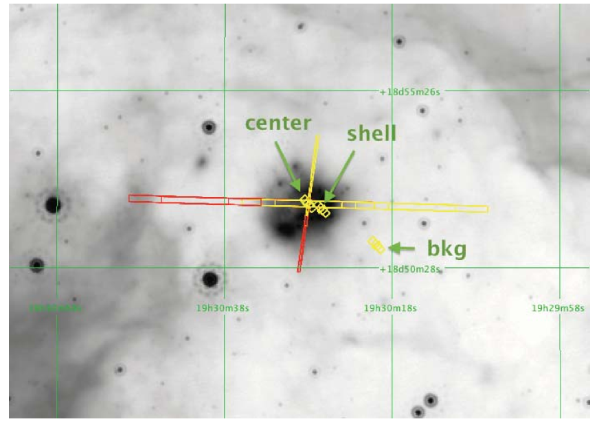
Figure 1: The Spitzer IRS slit superposed on a MIPS 24$\mu$m image of the SNR G54.1+0.3. The wide and long horizontal slits are the low-resolution LL1 (in red) and LL2 (in yellow) modules; the thin and long vertical slits are the low-resolution SL1 (red) and SL2 (yellow) modules. The high-resolution slits are the much smaller footprints shown in yellow; LH has a larger FOV than that of of SH. The positions of center, shell and background regions of high-resolution IRS spectra are labeled.

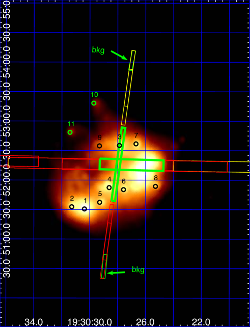
Figure 2: A close up of the low-resolution IRS SL1 (red, vertical), SL2 (yellow, vertical), LL1 (red, horizontal), and LL2 (yellow, horizontal) are marked on the Spitzer 24$\mu$m image. OB stars identified by Koo et al. (2008) and Kim et al. (2013) are labeled and the star behind the SL slits is object 3 (Koo et al., 2008) for which Kim et al. (2013) did not have spectroscopic confirmation. The regions for the extracted spectra are marked in green (thick) and the background regions for SL are marked in green (thin; the background (bkg) region marked in north is for SL2 and in south is for SL1.

Table 1: Summary of Far-IR and Submm Observations.

Date	Telescope	Wavelength	FWHM Beam
2006 Apr 18 and May 3-4	CSO SHARC-II	350$\mu$m	8.5′′
2008 Apr 27 and Jun 15	APEX LABOCA	870$\mu$m	18.6′′
2011 May 1	Herschel SPIRE	250, 350 and 500$\mu$m	18.1, 24.9 and 36.4′′
2012 April 9	Herschel PACS	70, 100 and 160$\mu$m	6, 8 and 12′′

2.2 Far-infrared and submm observations

2.2.1 Herschel

We used archival data from the Herschel Space Observatory (Pilbratt et al., 2010, hereafter Herschel) taken as part of the HiGAL Legacy survey (Molinari et al., 2010) for the Photodetector Array Camera (PACS; Poglitsch et al., 2010) 70 and 160 $\mu$m and the Spectral and Photometric Imaging Receiver (SPIRE; Griffin et al., 2010) 250, 350 and 500 $\mu$m images (Table 1). The observations are taken in parallel mode to maximize survey speed and wavelength coverage and the instruments wavelength multiplexing capabilities. We also created a PACS 100$\mu$m image using scan-map data from obsids of 1342231921 and 1342231922 (OT1_ttemim_1). PACS maps at wavelengths of 70, 100 and 160$\mu$m with a Full Width Half Maximum (FWHM) of 6, 8 and 12^′′ and SPIRE at 250, 350 and 500$\mu$m with FWHM of 18.1, 24.9 and 36.4^′′, respectively. Data are taken from the arrays simultaneously as the spacecraft is scanned across the sky. In order to have redundancy two passes are taken over the same region of the sky using the other scan angle at -42.5^∘ angle which is nearly orthogonal to the first one and the distance between each scan in parallel mode is set by the size of the PACS array.

The PACS and SPIRE photometric data were reduced with the Herschel Interactive Processing Environment (HIPE; Ott, 2010). For PACS, all low-level reduction steps were applied to Level 1 using HIPE and level 1 output was imported to scanamorphos software (Roussel, 2013) to remove effect due to thermal drift and uncorrelated noise of the individual bolometers. For the SPIRE data, additional iterative baseline removal step (Bendo et al. 2010) was applied and the final map was created with the standard naive mapper.

The flux calibration uncertainty for PACS is less than 10% (Poglitsch et al., 2010) and the expected color corrections are small compared to the calibration errors. We therefore adopt a 10% calibration error for the 70 and 160$\mu$m data. The SPIRE calibration methods and accuracies are outlined by Swinyard et al. (2010) and are estimated to be 7%. Note that we also examined Planck archival data (e.g., Planck Collaboration et al., 2011) but the emission from G54.1+0.3 could not be positively identified due to the large angular size of the Planck beam (4.4-32.7^′ from 857 to 30 GHz).

2.2.2 SHARC-II Data Reduction

Higher resolution observations of G54.1+0.3 at 350$\mu$m were provided by observations with SHARC-II (Table 1). SHARC-II is a 12$\times$ 32 bolometer array with field of view of $2.6^{\prime}\times 0.97^{\prime}$ on the Caltech Submillimeter Observatory in Hawaii. The Dish Surface Optimization System (DSOS) was used throughout the run, providing a stable beam with FWHM of 8.5^′′. The weather conditions were good during both runs, with $\tau_{225}$ ranging from 0.04 to 0.05. 22 scans were observed in total using the boxscan format with scanning speed of 20 scans per second with on-source integration time of 3.7 hours. The sources Callisto, Neptune, Arp220, G34.3 and Hebe were used for pointing, focusing and flux correction. The focus was found to be stable within 5 mm. Pointing was measured to be offset by $8^{\prime\prime}$, this was corrected in the data reduction. The data were reduced with the SHARC-II data reduction package CRUSH version 1.6.3 (Kovács et al., 2006). The background noise in the central region is $\sim$80 mJy beam^-1. The flux uncertainties include the flux calibration uncertainty, which is typically 15%.

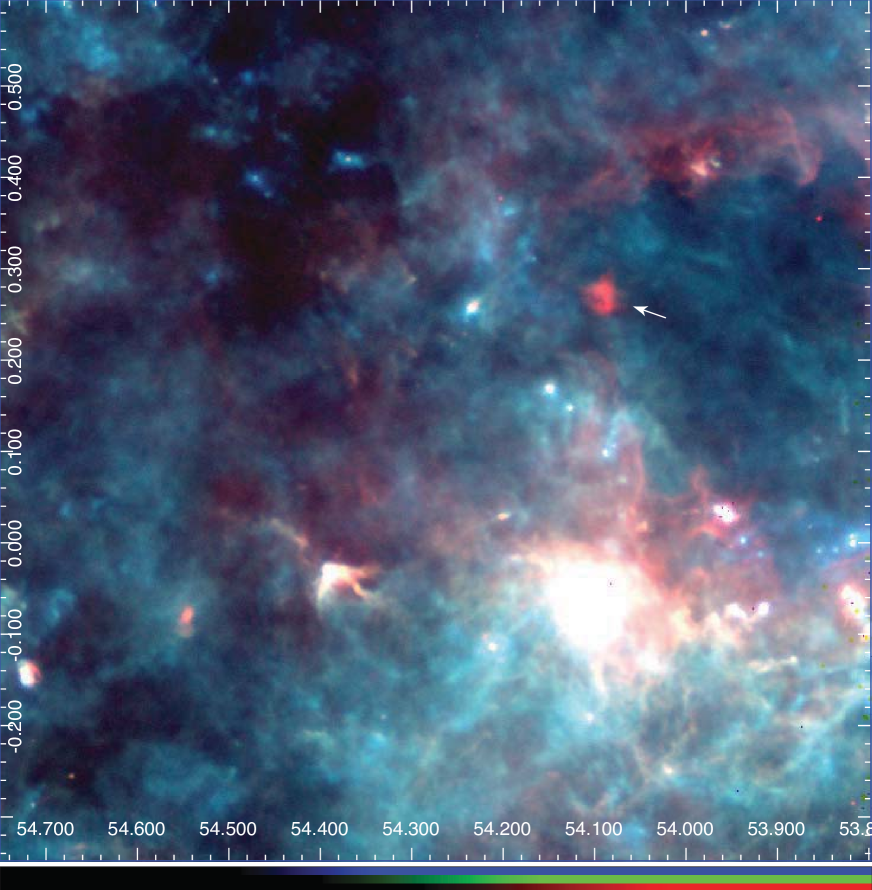
Figure 3: A Herschel three colour image of G54.1+0.3 and its environments. The emission at 70, 250 and 500$\mu$m is shown in red, green and blue, respectively (warmer material appears in redder color). The SNR G54.1+0.3 is marked as an arrow and is noticeably redder (warmer) than the ISM cirrus (in blue/green) and other emission in the immediate vicinity of the SNR. Galactic coordinates in degree are marked, and color bar scale is 0.004 - 0.75 Jy pixel^-1 (1 pixel = 1.4^′′) in red, 0.003 - 53 Jy beam^-1 in green, and 0.06-14 Jy beam^-1 in blue.

2.2.3 LABOCA Data Reduction

We supplemented the Herschel and SHARC-II data with 870$\mu$m observations taken with the LABOCA camera (Siringo et al., 2009), a 295-pixel bolometer array with beam size FWHM of 18.6^′′, located on the Atacama Pathfinder EXperiment telescope (Güsten et al., 2006) on Chanjantor in Chile (Table 1). The observations were carried out in raster spiral mode with forty scans, each providing a fully sampled map over $8\times 8^{\prime}$. The total on-source integration time was 4.7 hours. Two independent measurements of the optical depth, $\tau$ were obtained. The first method used the precipitable water vapor (PWV) levels measured every minute along the line of sight, then scaled using the relevant atmospheric transmission model. The PWV was low but variable, ranging from 0.5–0.8 mm. The second method calculated $\tau$ from skydip measurements, where a model of the dependence of the effective sky temperature on elevation were fitted to determine the zenith opacity. The two skydips taken before and after the on-source scans were both well fitted by the model, with $\tau$ between 0.16-0.19. These values were, on average, 30% lower than those estimated from the PWV measurements. A linear combination of the two methods, and a final comparison with the calibrator models (e.g. Siringo et al., 2009), was used to determine the values used in the data reduction.

The data were reduced using the BoA (BOlometer array Analysis software) package. The focus was checked on observations of Jupiter and G34.3 and were stable within $\pm$0.2 mm. Pointing observations of Jupiter were within $2^{\prime\prime}$ in azimuth and elevation. Bad and noisy pixels were flagged. The data were de-spiked and correlated noise was removed (removing a large fraction of the sky noise Schuller et al., 2009). The reduction was optimized for the recovery of weak sources. All of the scans were coadded (weighted by rms^-2) to create the final map. After a first iteration of the reduction, the source map was used to flag bright sources and the data were reduced again. This was efficient at removing negative artifacts which appeared around the bright sources in the first iteration and led to a more stable background noise level in the central region ($\sim$10 mJy beam^-1). The calibrators Jupiter, G34.3, J1925+211 and J1751+097 were used to calibrate the map. The total uncertainty in the calibration, including uncertainties in the calibrator model is $\sim$12%.

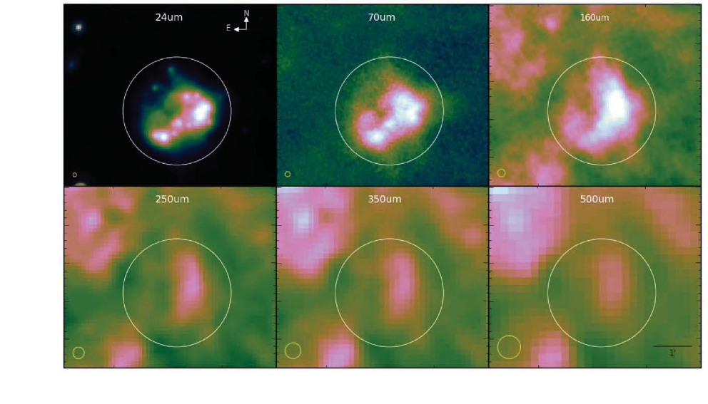
Figure 4: Comparison of Spitzer and Herschel images of G54.1+0.3. Top: Spitzer 24$\mu$m  (left), Herschel PACS 70$\mu$m (middle) and 100$\mu$m (right). Bottom: Herschel SPIRE 250$\mu$m (right), 350$\mu$m (middle) and 500$\mu$m (right). Beam sizes are shown in the lower right corner, the large circle has a radius 86^′′ centered on R.A. $19^{\rm h}30^{\rm m}28.42^{\rm s}$ and Dec. $+18^{\circ}$52${}^{\prime}6.6^{\prime\prime}$ (J2000). The dust emission in the PACS and SPIRE images is distributed in a shell-like morphology, similar to that seen in the Spitzer 24$\mu$m image (tracing warm dust). The shell-like morphology in the PACS images is elongated from left to right, but the emission in the SPIRE images (tracing colder dust) is elongated from north to south with a structure similar to the emission seen in the Spitzer 8$\mu$m image.

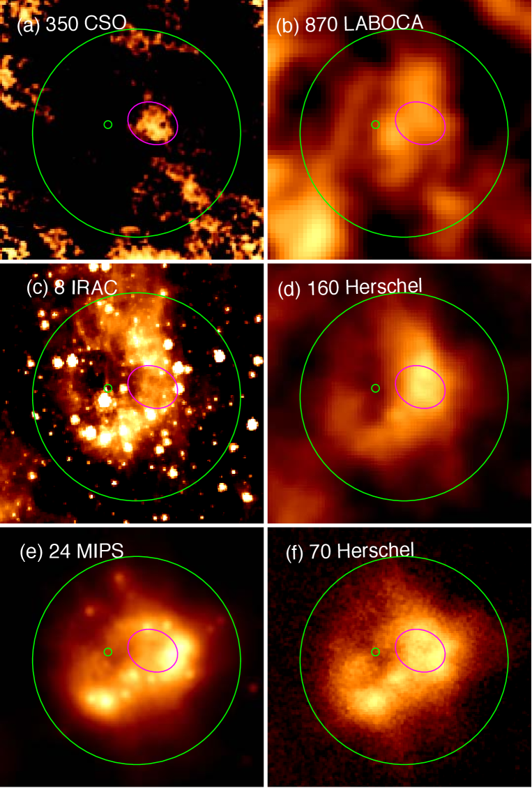
Figure 5: High resolution submm and mid-IR images of G54.1+0.3. (a) CSO SHARC-II at 350$\mu$m (the color scale ranges 0.05 – 0.33 Jy beam^-1). (b) LABOCA at 870$\mu$m (7$\times$10^-5 – 0.36 Jy beam^-1). (c) Spitzer IRAC 8$\mu$m (15-21 MJy sr^-1), and (d) Herschel PACS 160$\mu$m (0.017 – 0.045 Jy pixel^-1). (e) Spitzer IRAC 24$\mu$m (53-224 MJy sr^-1), and (f) Herschel PACS 70$\mu$m (0.007 – 0.028 Jy pixel^-1). The SHARC-II submm image (note that this observation was taken earlier than those from Herschel as listed in Table 1) reveals submm emission from cold dust in G54.1+0.3 (marked as a purple circle), which coincides the bright part of the Herschel 350$\mu$m image in higher spatial resolution. The small and large circles (in green) mark the locations of the pulsar J1930+1832 and the entire SNR, respectively (Lang et al., 2010).

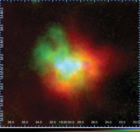
Figure 6: Three color image of G54.1+0.3 with blue, green and red colour indicating X-ray, radio and FIR (Herschel PACS at 70$\mu$m) emission respectively. The Herschel image shows a torus-like shell emission (15^∘ tilted from the horizon) and consistent with the 24$\mu$m emission. The radio pulsar nebula is perpendicular to this torus structure. The Herschel images (see Figure 4) also show an emission feature extended north of this shell on the western side of the remnant. The north is up and the west is right. Color bar scale is 0.62 - 13.20 $\times$10^-6 photons cm^-2 s^-1 in blue, 0.15 - 1.75 MJy sr^-1 in green, and 0.004 - 0.75 Jy pixel^-1 (1 pixel = 1.4^′′) in red.

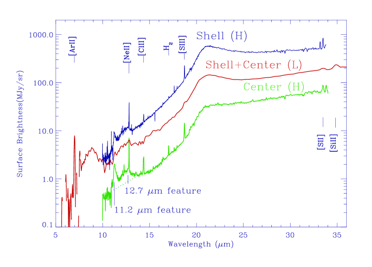
Figure 7: Spitzer IRS spectra of G54.1+0.3. The red curve is the low-res spectrum and the blue is from the high-res spectrum from the shell component of the SNR (the bright ‘blob’ emission in the southwestern shell). The green curve is the high res spectra measured in the central region. The line at 14.35$\mu$m shows multiple (high velocity) components in emission as listed in Table 2.

3 Results

3.1 G54.1+0.3 in Many Colours

Here we discuss the appearance of the SNR in the IR-submm. A three color FIR-submm Herschel image (70$+$350$+$500$\mu$m) in Figure 3 shows the dust structures in the local area. The SNR itself can be seen at the center of this image and is noticeably redder (hotter) than the immediate surroundings, suggesting that the 70$\mu$m emission is indeed associated with the remnant. H II regions and young stellar objects are instead bright in all three bands, and appear white in this image, with interstellar cirrus from unrelated foreground and background dust emission appearing blue.

Zooming in on the remnant, the MIR images (Figure 5), show bright emission from a shell-like structure (hereafter the shell) located at the southern end of the radio emission, with peak brightness in the western side. We see IR emission extending north from the western peak of the shell. In Figure 4, we next compare the Spitzer MIR data to the FIR images. At long wavelengths ($\lambda>100$$\mu$m), we see a slight change to the distribution of the IR emission: the eastern part of the shell begins to fade in brightness and the northern elongated structure becomes more prominent. This feature is particularly obvious when we resolve the Herschel emission in the higher resolution LABOCA 870$\mu$m image (Figure 5), though the peak emission in the LABOCA image is slightly offset towards the pulsar location compared to the 24 and 70$\mu$m emission. The elongated northern structure seen in the Herschel and LABOCA data is coincident with the same structure seen in the IRAC 8$\mu$m image (Figure 5). The SHARC-II 350$\mu$m image provides us with a means to resolve out the submm emission seen with Herschel at 350$\mu$m: here we see a smaller structure coincident with the brightest peaks in the 24, 70 and 160$\mu$m images (in the western part of the shell). The detection of submm and far-IR detection from G54.1+0.3 and its coincidence with the IRAC 8$\mu$m emission (western peak and elongated north west structure) and the Spitzer 24$\mu$m (shell structure) hints that the FIR emission could originate from cold dust associated with the SNR (we return to this in Section 4). The CSO SHARCII submm image at 350$\mu$m has a factor of 3 higher spatial resolution compared to the SPIRE image at 350$\mu$m, and the SHARCII image shows small scale structures that resemble those in the 8$\mu$m image (see Figures 5a and 5c).

In Figure 6 we compare the FIR emission with the well studied X-ray and radio data for G54.1+0.3 using archival Chandra and Very Large Array (VLA, 4.45 GHz) observations. In X-ray we see the pulsar at the center and the pulsar wind nebula extending east - west (e.g Lu et al., 2002). In radio, we see many different structures including lobes, filaments, and diffuse emission (see Lang et al., 2010 for more information). The radio emission in general extends perpendicular to the X-ray with a narrow ‘waist’ region at the center coincident with the X-ray diffuse structure. We also see asymmetry in the radio emission with the remnant appearing brighter in the south. The ‘double-pronged’ feature in the north appears jet-like. (We note that we see no radio feature coincident with the pulsar, Lang et al., 2010.) When we compare with the FIR emission (using Herschel 70$\mu$m, bottom left, red) we see that the bright FIR shell-like emission is distributed to the south of the X-ray emission and on the southern edge of the diffuse radio that traces the pulsar wind. Figures 4 and 6 show clearly that the FIR/submm structure that extends north from the shell on the western side also encompasses the X-ray and radio at the center, tracing the outer edge. Lang et al. (2010) suggested that the IR shell-like emission was due to the interaction of the PWN with an interstellar cloud. In contrast, Temim et al. (2010, 2017) suggested that the PWN is driving shocks into an expanding SN ejecta. The structure seen in Figure 6 is remarkably similar to that of the Crab Nebula where the FIR emission also surrounded the inner radio and X-ray emission (Gomez et al., 2012b). In that work, the FIR emission was shown to originate from dust formed in the SN ejecta and not due to the interaction with circumstellar or interstellar material despite being brighter in the outer regions of the X-ray and radio emission. They suggested that the Crab Nebula does not have a forward shock such that the pulsar wind nebula is able to expand into the freely expanding SN ejecta (Hester, 2008; Smith, 2013). As well as a low interstellar density surrounding the Crab, this can be explained if the Crab was the result of a low-energy Type IIn-P event from a relatively low mass star (Smith, 2013). In this scenario the SN ejecta interacts with a thin shell of circumstellar material and the expansion of the pulsar wind nebula accelerates and fragments the Crab filaments. Given that the PWNs within G54.1+0.3 and the Crab Nebula have shown to be similar (Kim et al., 2013), we now posit in this work that a similar mechanism (dust formed in the ejecta material) could be responsible for the IR-submm appearance of G54.1+0.3. Based on spectral ejecta lines and dust features similar to that of Cas A, we interpret the IR emission is from ejecta and associated dust. However, since the spectral coverage is limited, we can not rule out contribution from interactions of PWN with interstellar clouds. We will return to this in Sections  3.2 and 4 for details.

3.2 Ejecta Lines and Dust from MIR spectroscopy

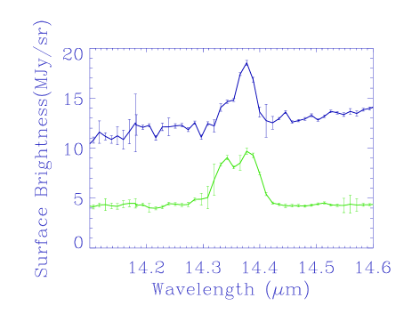
Figure 8: Line width of the [Cl II] emission seen at 14.36$\mu$m. The spectra from the shell and central regions are shown in blue and green, respectively. The line shows multiple (high velocity) components in emission (the two-component gaussian fits listed in Table 2).

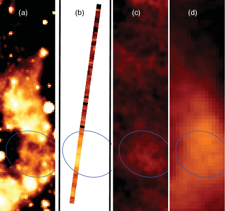
Figure 9: Comparison of Ar line and continuum maps: (a) Spitzer IRAC 8$\mu$m image, (b) [Ar II] at 6.99$\mu$m image produced using the IRS data (in staring mode;i.e., a IRS slit) observation after the continuum is subtracted, (c) CSO SHARCII 350$\mu$m image, and (d) Herschel 160$\mu$m image. The SHARCII 350$\mu$m emitting region is marked as an ellipse. The [Ar II] image shows the ejecta morphology similar to the IRAC 8$\mu$m image and SHARCII 350$\mu$m dust emission within the elliptical region, and [Ar II] ejecta emission is correlated to the dust emission. Note that SHARCII 350$\mu$m image (c) has a factor of 1.5 higher spatial resolution to that of the Herschel 160$\mu$m image (d).

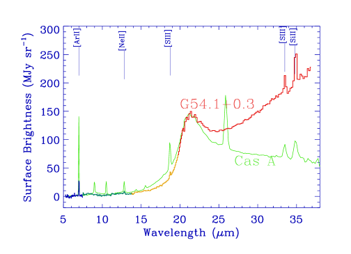
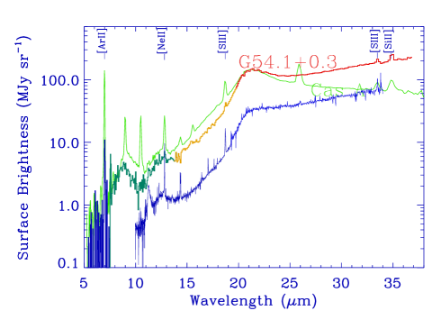
Figure 10: Comparing the Spitzer IRS MIR spectrum for G54.1+0.3 with Cas A. The 21$\mu$m dust feature of G54.1+0.3 is similar to that of Cas A, showing that the feature is unique dust originated from supernovae. The spectra shown on log-scale highlights the dust feature seen at $\sim$12.7$\mu$m (between 10 and 14$\mu$m) in the low res spectrum (SL in green, LL2 in yellow and LL1 in red) and the ‘sharper’ dust feature at 11$\mu$m seen in the high resolution spectrum (in blue) of G54.1+0.3.

3.2.1 Supernova Ejecta Lines

Table 2: Observed Spectral Line Brightness from Spitzer IRS spectrum. ^a - The spectral lines are fit with two (2) or one (1) Gaussian component(s) (Figure 7).

Region	Wavelength	Line	FWHM	Surface Brightness	De-reddened S.B.	Velocity	Shift
	($\mu$m)		$\mu$m	(erg s-1 cm-2 sr-1)	(erg s-1 cm-2 sr-1)	(kms-1)	(kms-1)
shell	6.9911$\pm$ 0.0012	[Ar II]	0.0682$\pm$ 0.0033	1.30($\pm$0.07)E-04	1.43($\pm$0.08)E-04	…	…
(lowres)	12.8231$\pm$ 0.0065	[Ne II]	0.1481$\pm$0.0169	6.49($\pm$0.77)E-06	7.68($\pm$0.90)E-06	…	…
	18.7338$\pm$ 0.0021	[S III]	0.1302$\pm$ 0.0058	9.27($\pm$0.41)E-6	1.11($\pm$0.05)E-05	…	…
	33.5004$\pm$ 0.0062	[S II]	0.2599$\pm$ 0.0100	2.12($\pm$0.81)E-05	2.31($\pm$0.09)E-05	…	…
	34.8920$\pm$ 0.0023	[Si II]	0.3055$\pm$ 0.0086	5.13($\pm$0.14)E-05	5.55($\pm$0.15)E-05	…	…
shell (2a)	14.3374$\pm$0.0051	[Cl II]	0.0173$\pm$0.0213	6.34($\pm$0.78)E-07	7.13($\pm$0.88)E-07	384$\pm$447	-634$\pm$107
(hires)	14.3748$\pm$0.0028		0.0331$\pm$0.0074	3.18($\pm$0.71)E-06	3.58($\pm$0.80)E-06	680$\pm$153	129$\pm$58
shell (1a)	14.3729$\pm$0.0066	[Cl II]	0.0399$\pm$0.0167	3.51($\pm$1.46)E-06	3.95($\pm$1.64)E-06	832$\pm$348	106$\pm$137
center (2a)	14.3347$\pm$0.0013	[Cl II]	0.0185$\pm$0.0039	2.08($\pm$0.44)E-06	2.34($\pm$0.49)E-06	386$\pm$081	-690$\pm$30
(hires)	14.3801$\pm$0.0022		0.0371$\pm$0.0057	3.70($\pm$0.57)E-06	4.16($\pm$0.64)E-06	777$\pm$118	+254$\pm$46

The Spitzer IRS spectra include a set of low-res spectra (L, resolving power of 65-120) towards the southwestern shell and two sets of high-res (H, resolving power of 600) spectra toward the center and the southwestern shell (Figure 7). The low-res IRS spectra show bright [Ar II] emission at 6.9$\mu$m, [Ne II] at 12.8$\mu$m, [S III] at 18.7 and 33.5$\mu$m, and [Si II] at 34.89$\mu$m.

The surface brightnesses of the low-res lines are corrected for extinction using $N_{H}=1.6\times 10^{22}\,\rm cm^{-2}$ from X-ray measurements (Lu et al., 2002) (see Table 2). The line brightnesses of high-res spectra were listed in Temim et al. (2010). Our estimate shows that the emission seen in the IRAC 8$\mu$m image (see Figure 5) is composed of Ar ejecta at 20 percent and 9$\mu$m broad dust feature at 80 percent using the IRS low-res spectrum after convolving the IRAC transmission curve (see Figure 1 of Reach et al. 2016). The 9$\mu$m broad dust feature is fit with silica dust and is associated with the SN ejecta (see Section 4.2 for details).

We also detect the [Cl II] line at $\sim$14$\mu$m. The rest wavelength of this line (14.3678$\mu$m) is very close to [Ne V] (14.3217$\mu$m), though we do not detect any emission from [Ne V] in the expected 24.3$\mu$m line. The line profile for [Cl II] is shown in Figure 8. Although it is not resolved in the low-res spectrum, the high-res IRS spectrum resolves the line into two velocity components seen in both the shell and central regions of the SNR. We fit them using two gaussians and the central velocities and widths with their errors are given in Table 2; both spectra show that the two knots are located at the central velocity of $-650\rm\,km\,s^{-1}$ (located at the front side of the SNR) and $\sim$200$\rm\,km\,s^{-1}$ (located at the backside of the SNR), and their widths are $\sim$380 kms^-1 and $\sim$700 kms^-1, respectively, which indicates that they are high velocity ejecta knots. This is different from Temim et al. (2010) who measured the velocity using high-res spectra and found a single gaussian component was adequate. The low-res spectra used here covers regions that were not covered in their analysis and demonstrate different line profiles requiring multiple-components. Combined, this work indicates there are at least two ejecta clumps of the fast-moving ejecta material existing in different places along the line of sight.

Interesting dust features are seen at 21 and 9$\mu$m; the former is a smooth peak increasing in flux up to 21$\mu$m and decreasing beyond this. Another dust feature appears as a bump at 11.3$\mu$m (10-13$\mu$m). The high-res spectra shows that the feature has additional peak at 11.2$\mu$m (see next Section). The IRS spectrum (Figure 7) indicates that Spitzer IRAC 8$\mu$m map in Figure 5 is from a combination of the Ar eject map and the 9$\mu$m dust.

Understanding the correlation between dust and Ar ejecta requires spectral mapping to cover the entire SNR as it was done for Cas A (Rho et al., 2008; Smith et al., 2009). Unfortunately, such data are not available for G54.1+0.3. We still generated the Ar image shown in Figure 9b by using the IRS staring mode (one slit) after subtracting the continuum by spectral fitting. The [Ar II] image is compared to the Spitzer 8$\mu$m , CSO SHARCII image at 350$\mu$m and Herschel 160$\mu$m image. The [Ar II] ejecta shows a morphology similar to the SHARCII 350$\mu$m dust emission (see Figure 9), indicating that the Ar ejecta are associated with the dust. The IRAC 8$\mu$m image shows small-scale structures similar to those in the SHARCII image at 350$\mu$m whereas the image shows large-scale structures similar to those in the Herschel 160$\mu$m cold dust map, in particular, in the northwestern shell. The IRAC 8$\mu$m image seems to contain not only Ar ejecta emission but also additional continuum emission which may be associated with a combination of cold and warm dust.

There is additional supporting evidence that the Ar ejecta of G54.1+0.3 might be associated with dust based on the analogy of the SNR G54.1+0.3 to Cas A. Both G54.1+0.3 and Cas A show a 21$\mu$m dust feature (see §3.2.2 for details, see Figure 7), and the map of Ar ejecta in Cas A is remarkably similar to the 21$\mu$m dust map where dust is formed in the SN ejecta (see Figure 2 of Rho et al., 2008). The element Ar is one of the oxygen burning products at the inner-oxygen and S-Si layers, with the 21$\mu$m-peak dust forming around these nucleosynthetic layers (e.g., Woosley & Weaver, 1995, Rho et al., 2008; Nozawa et al., 2003, see more discussion in).

In the Crab Nebula, the dust is found to be associated with the ejecta (Gomez et al., 2012c, and references therein). We suggest that in SNR G54.1+0.3, the dust is also associated with the ejecta. The analogy of the SNR G54.1+0.3 to the Crab Nebula, where the infrared and optical/infrared shells show overabundant ejecta knots, and the high resolution images show almost one-to-one correspondence between ejecta and dust knots with prominent finger-shaped knots caused by Rayleigh-Taylor instabilities (more discussion in Section 4; Hester, 2008; Jun, 1998), suggests that the ejecta of G54.1+0.3 are likely associated with the dust. Hopefully, future spectral mapping such as with JWST will further confirm the correlation between the ejecta and dust for the entire SNR of G54.1+0.3.

3.2.2 21$\mu$m dust feature: a dust twin of Cas A

As well as ejecta lines, as discussed in the previous Section, the low-res spectra show a strong dust feature peaking at 21$\mu$m, with additional (weaker) dust features at 8.5$\mu$m and 10 - 14$\mu$m. In Figure 10, we compare the IRS spectrum of Cas A from Rho et al. (2008) with G54.1+0.3 and find that the 21$\mu$m dust feature is remarkably similar to that seen in Cas A. (Unlike Cas A, G54.1+0.3’s flux continues to rise well beyond the 21$\mu$m peak.) Historically, the term ‘21$\mu$m dust feature’ was allocated to the spectral feature seen in carbon-rich post-asymptotic giant branch (post-AGB) stars (Sloan et al., 2014), evolved stars (Kwok et al., 1989) and protoplanetary nebulae (PPNe, Volk et al., 2011; Jiang et al., 2005); this feature is often accompanied by a peak at 30$\mu$m (see also Figure 11). However, note that the historical 21$\mu$m feature actually peaks between 20-20.3$\mu$m (Kwok et al., 1989; Li et al., 2013; Cerrigone et al., 2011). We distinguish this feature (we call $``$20$\mu$m dust feature”) from our 21$\mu$m feature observed in the SNRs of G54.1+0.3 and Cas A.

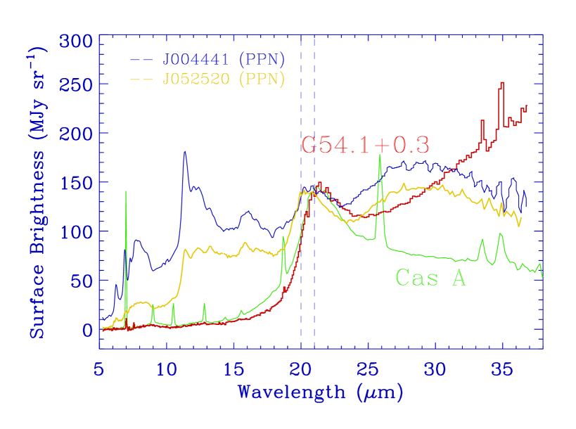
Figure 11: Comparing the MIR spectrum for G54.1+0.3 with Cas A and PPNe from Volk et al. (2011). The dotted vertical lines indicate wavelengths of 20 and 21$\mu$m. Both G54.1+0.3 and Cas A have dust peaks at 21.1$\mu$m (the smooth bump) whereas the PPNe (J004441 and J052520) have a dust-peak feature at 20.1$\mu$m as well as broad features at 10-17$\mu$m and at 25-35$\mu$m.

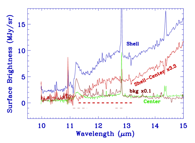
Figure 12: Spitzer IRS spectra of G54.1+0.3. The red curve is the low-res spectrum including bright emission at the shell. The blue curve is the high-res spectrum from the shell component of the SNR (the bright ‘blob’ emission in the southwestern shell), the green is the high-res spectrum measured in the central region, and the brown is the high-res spectrum from the background (bkg) region. The slit locations are shown in Figure 1. The line at 14.35$\mu$m shows multiple (high velocity) components in emission as listed in Table 2. The spectra show dust features at 9, 10-14 (marked in the dotted line in green), and 21$\mu$m and a narrow dust feature at 11.2$\mu$m.

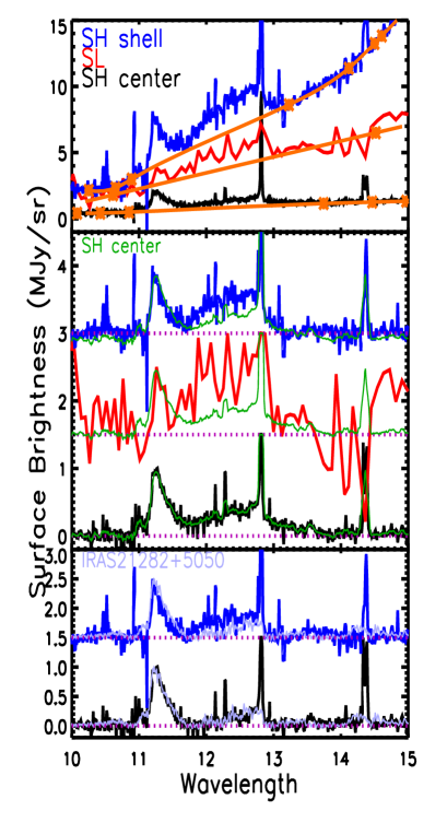
Figure 13: A closer look to the SH and SL spectra of G54.1+0.3 in the 10-14 $\mu$m region. (a: top) The SH and SL spectra with their adopted continua (and chosen continuum points): a global spline continuum (orange) and a local spline continuum (light blue; see text for details). (b: middle) A comparison of the continuum subtracted spectra using the global spline continuum, normalized to the strength at 11.2 $\mu$m (the [NeII] emission line is cut off for clarity). The spectra are offset from each other by 1.5 units. For reference, a smoothed version of the continuum subtracted SH center spectrum is over-plotted in green. (c: bottom) A comparison of the PAH emission features in this wavelength range (using a local spline continuum) for the SH spectra (shell in blue and center in black) of G54.1+0.3 with the spectrum of the planetary nebula IRAS21282+5050 (in light blue; taken from Hony et al., 2001), normalized to the peak intensity of the 11.2 $\mu$m PAH band (the [NeII] emission line is cut off for clarity). The spectra are offset from each other by 1.5 units.

Comparing the Spitzer spectra of the two SNRs with PPNe from Volk et al. (2011) (Figure 11), we see that the PPN feature is offset by $\sim$1$\mu$m from the 21.1$\mu$m dust feature in G54.1+0.3 and in Cas A. Unlike the PPNe, neither SNR has a broad dust bump at 30$\mu$m, though they do have weaker dust features between 10-15$\mu$m (see Section 3.2.3). The 21$\mu$m dust feature therefore seems to be unique to the two young SNRs of Cas A and G54.1+0.3 to date. We will return to the dust composition responsible for this feature in Section 4.

3.2.3 11$\mu$m dust features

Weaker dust features are seen in the IRS spectra in the 10-14$\mu$m range (Figures 1 and 10). In particular, a broad emission feature is present ranging from approximately 10.5 to 14$\mu$m with, on top of it, a strong distinct feature at 11.2 $\mu$m. The broad feature is much more noticeable in the shell spectrum when we subtract the center spectrum after scaling the spectra with the sharp 11.2$\mu$m feature as shown in Figures 12 and 13a. To investigate this emission, we apply a global spline continuum with anchor points shortward of 11$\mu$m and longward of 13 $\mu$m (Figure 13a). The overall shape of the 10-14 $\mu$m emission is similar in the two SH spectra while the strength of both the broad emission feature and the distinct 11.2 $\mu$m feature varies (Figure 13b). While less clear in the SL spectrum due to the lower S/N and spectral resolution, we note that the 10-14 $\mu$m emission features are very similar to those in the SH shell spectrum when allowing for a scaling factor of 0.6 to match the strength of the dust continuum emission. (The relative strength of the broad emission feature and the 11.2 $\mu$m band is slightly different.) A comparison with the SL data of Cas A reveals that this broad emission component is also present in Cas A, albeit at a weaker level, while the distinct feature at 11.2$\mu$m seems to be absent (Figure 10).

The distinct feature at 11.2 $\mu$m is reminiscent of the 11.2 $\mu$m emission band due to Polycyclic Aromatic Hydrocarbon molecules (PAHs). To explore a possible PAH origin, we follow Hony et al. (2001) and apply a local spline continuum: in addition to the anchor points used for the global spline continuum, two additional anchor points at approximately 11.7 and 13 $\mu$m are used (Figure 13, top panel). We compare the resulting continuum subtracted SH spectra with the PAH emission seen in the sample of Hony et al. (2001).

The emission seen towards the SH center position is nearly identical to the PAH emission of the planetary nebula (PN) IRAS21282+5050: at the position of the 11.0, 11.2 and 12.7$\mu$m PAH bands in the PN, the SH center spectrum shows emission bands with almost identical shape, e.g., the 11.2$\mu$m PAH feature. A small discrepancy is also seen at the transition from the 11.0 to the 11.2 $\mu$m PAH bands (the 11.0 $\mu$m as a shoulder attached to the 11.2 $\mu$m band versus two more distinct bands). Both PAH profiles have been seen in a variety of objects and within extended sources (e.g. Boersma et al., 2013). The observed emission towards the SH center position (when subtracting a local spline continuum) is thus consistent with an origin in PAH emission. Note that the spectrum at the center was already background subtracted using the background position 2.5 arcmin away as shown in Figure 1.

The SH shell spectrum clearly exhibits the 11.2 $\mu$m PAH band and lacks emission near 11.0 and 13.5 $\mu$m. The 11.0 $\mu$m is a weaker PAH band attributed to ionized PAHs (Hudgins & Allamandola, 1999) and thus is only seen for a significant PAH ionization fraction. Hence, the lack thereof poses no problem to a PAH origin of the 11.2 $\mu$m emission. The emission in roughly 11.8 to 13 $\mu$m is somewhat unusual from a PAH perspective. Clearly, this emission can be consistent with the presence of a 12.7 $\mu$m PAH band (at various strengths). However, typically, this feature ranges from roughly 12.2 to 12.9 $\mu$m and a weaker PAH band at 12.0 $\mu$m is discernible (i.e. not blended) when present (see the PN shown in Figure 13 or Figure 7 of Hony et al., 2001). Note that a typical PAH emission spectrum ranges between 10 and 15 $\mu$m.

In contrast, the SH shell spectrum exhibits a smooth increase in surface brightness starting from $\sim$11.7 $\mu$m up to $\sim$13 $\mu$m. A similar profile is seen towards one or two $\beta$ objects in the sample of Matsuura et al. (2014, see their Fig. 14, e.g. IRAS05360-7121). Therefore, we conclude that the observed 11.2 $\mu$m feature is consistent with an origin in PAH emission while an origin of (some of) the 11.7-13 $\mu$m in PAH emission is possible, yet uncertain.

While PAH emission is thus present in these SH spectra, we note that the SH background spectrum exhibits typical and much stronger PAH emission. This is well illustrated in Figure 12. The 11.0, 11.2 and 12.7 $\mu$m  PAH emission bands are clearly present and resemble a typical PAH emission spectrum (see Figure 13). However, this background PAH emission is much stronger than that detected on-source: the 11.2 $\mu$m PAH intensity in the on-source spectra accounts for 6 and 20% of that seen in the SH background, respectively, for the center and shell position. The background observation is taken in staring mode, resulting in a FOV of 18.4″x 4.6″(8$\times$2 pixels). With a PSF corresponding to 2$\times$2 pixels, we investigate possible variability along the short slit and only find variation up to the 3% level. However, the background region is 2.5 arcmin away from the source. We therefore searched the Spitzer archive for other IRS observations in the vicinity to check for possible background variability on a larger scale and only found one SL observation. Unfortunately, discrepancies between the PAH band intensities between SL and SH observations (see e.g. Fig. 3 of Peeters et al., 2017) exclude a comparison of the 11.2 $\mu$m PAH band intensity between SH and SL observations at the 20% level, as required by our on-source observations. Given the proximity of the center and shell position to each other (the center positions of the two slits are 25^′′ apart and the slit coverages are next to each other as shown in Figure 1), we assume similar background emission for both positions. In that case, the maximum residual background emission is given by the strength of the PAH emission seen in the center position. When the spectrum of the shell position is corrected for this possible remaining residual PAH emission, it still exhibits clear PAH emission (in particular the 11.2 $\mu$m band, see Figure 12).

PAH emission gives rise to a number of emission bands, the major ones centered at 3.3, 6.2, 7.7, 8.6 and 11.2 $\mu$m. We thus expect to see the 6.2, 7.7 and 8.6 $\mu$m PAH bands as well towards the shell. Unfortunately, these bands are located in the SL wavelength range where the data are of significantly lower quality and we do not detect any emission in SL2 (5.5-8.5 $\mu$m) except from the [ArII] and potential [Ni I] lines. We compared our SL spectrum with the IRS spectrum from a well-known PAH source, the reflection nebula NGC 7023, by normalizing its spectrum so that the integrated strength of the 11.2$\mu$m PAH band equals that observed in the SL shell spectrum (Figure 10). Given the strength of the 11.2 $\mu$m PAH band in the SL spectrum, we should have seen PAH emission at 6.2 and 7.7 $\mu$m since they are above the noise level. If born out that the 11.2$\mu$m PAH emission belongs to the SNR, this would be the first detection of PAHs associated with SN ejecta. This challenges both observations and theoretical models; none of the molecule and dust formation models mentioned above have predicted formation of PAHs in SN ejecta.

We extract the profile of the broad emission component by subtracting the emission seen towards the center from that towards the shell with the former scaled such that the integrated intensity of the 11.2 $\mu$m PAH band is equal to that in the shell. This implicitly assumes the band profile does not change between the two positions. The resulting profile is a smooth, symmetric feature from roughly 11.5 to 13 $\mu$m shown in Figure 12. A comparison is made between the center/shell/background + shell-center which is well fitted by a Gaussian with peak position of 12.3 $\mu$m and a FWHM of 1.1 $\mu$m. Possible carriers of this broad emission feature are PAHs or PAH-related species and SiC grains.

The 11.2 and 12.7 $\mu$m PAH bands are typically located on top of a broad emission plateau ranging from roughly 10.5 $\mu$m to roughly 14.5 $\mu$m. While this broad emission plateau shows little variation towards ISM-type sources (see e.g. Fig. 12 in Peeters et al., 2017), large variability is seen towards evolved stars exhibiting PAH emission (Sloan et al., 2014; Matsuura et al., 2014). Comparing a typical ISM-like PAH plateau with the broad emission feature seen in the SNR shows that the latter is considerably more narrow. We explore the possibility that the broad dust feature between 10-14$\mu$m is from SiC, with spectral fitting described in Section 4 (see Figures 16 and 17).

3.3 Warm and Cool Dust Distribution

We have generated temperature and dust mass maps using 0.2^∘ $\times$ 0.2^∘ cutouts of the 24$\mu$m, 70$\mu$m, 160$\mu$m, 250$\mu$m, 350$\mu$m, and 500$\mu$m maps. We have re-gridded the maps that are aligned to the same pixel grid, with 6^′′ pixels, and smoothed each map to the 36^′′ resolution of the 500$\mu$m image, and fit a simple 2-component modified black-body spectral energy distribution (SED) to each pixel.

Table 3: FIR-submm Flux Densities. ^a - The flux is measured within a circular aperture (with a radius of 90^′′) to cover the entire SNR except CSO. Since CSO has a limited field of view, we measured the flux from a circular aperture with the 22^′′ radius (centered on R.A. $19^{\rm h}30^{\rm m}25.5^{\rm s}$ and Dec. $18^{\circ}$ 52${}^{\prime}13^{\prime\prime}$, J2000; this is close to the intensity peak of 70$\mu$m image as shown in Figure 5.)

Data	Wavelength	Flux Density
	($\mu$m)	(Jy)
Herschel PACS	70	91.32$\pm$11.41
Herschel PACS	100	70.32$\pm$10.45
Herschel PACS	160	29.99$\pm$14.95
Herschel SPIRE	250	15.08$\pm$3.29
Herschel SPIRE	350	3.48$\pm$2.07
Herschel SPIRE	500	3.32$\pm$1.43
CSO SHARCIIa	350	1.50$\pm$0.30
APEX LABOCA	870	0.25$\pm$0.04

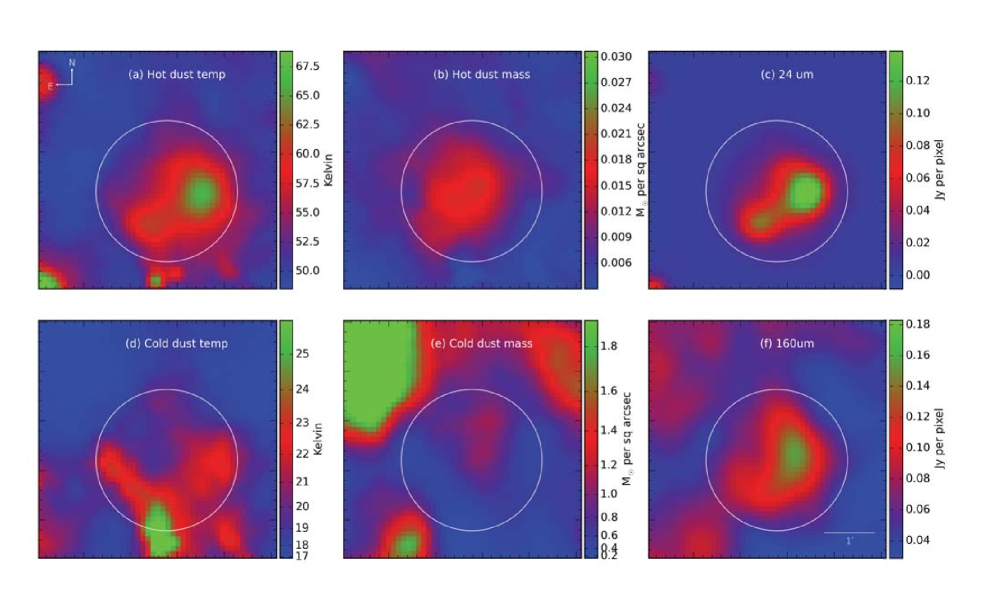
Figure 14: Temperature and dust mass maps of G54.1+0.3 for the hot and cold components with Spitzer 24$\mu$m and Herschel PACS 160$\mu$m maps. (a) Hot dust temperature map has a range of 50-68 K, (b) Hot dust mass map has a range of 0.006-0.02 M_⊙ per arcsec. (c) Spitzer 24$\mu$m image, (d) Cold dust temperature map has a range of 18-25 K, and note northeastern shell has a low temperature of 18-20 K, (e) Cold dust mass map has a range of 0.4-1.4 M_⊙ per arcsec and shows cold dust is concentrated on the northern part of the SNR and (f) Herschel PACS 160$\mu$m image.

This method will distinguish between warm and cool dust components. We note that a more physical model would account for multiple temperature components, though in terms of deriving dust masses, the assumption of two components makes only a factor of  2 difference in the derivation of dust mass (see Mattsson et al., 2014). The fitting was performed using a chi-squared-minimizing routine which incorporates the color-corrections for filter response function and beam area (see Gomez et al. 2012b for details), assumed an emissivity slope of $\beta$=2.0 and used a dust mass absorption coefficient of $\kappa$ at 500$\mu$m = 0.051 kg m^-2 (Clark et al., 2016). Note that for a pixel with an SED that is best fit by a single-component model (such as pixels with foreground cirrus only), this method will effectively yield a $`$second’ component with no mass (i.e., negligible mass with a large uncertainty, compatible with zero).

Figure 14 shows temperature and dust maps of the hot and cold components. The hot dust mass is concentrated toward the central area (slightly to the west) and the cold dust mass is concentrated to the northern and central parts of the SNR; the maps are consistent with the difference between the 24$\mu$m and 160$\mu$m images. The temperature where the cold dust mass is concentrated ranges from 18 to 25 K as shown in Figure 14d, and the cold temperature extends as low as $\sim$18 K in the northeast direction where a thin shell exist in the infrared maps (in all bands). We have attempted to produce dust mass and temperature maps with a higher (18^′′) spatial resolution using Herschel super-resolution maps (e.g. at 500$\mu$m) and removed synchrotron emission using a radio map. However, no additional information was obtained from that exercise, and because the SNR G54.1+0.3 is small, the high-resolution maps may contain artefacts. We conclude that the low-resolution maps were sufficient for this purpose.

We compare our temperature maps with those by Temim et al. (2017). We note that Temim et al. (2017) used observations from 15$\mu$m to 100$\mu$m for their temperature maps with a resulting spatial resolution of 12^′′ and were able to fit only a single dust component. In contrast, we used maps from 24 to 500$\mu$m where the longer wavelength maps are sensitive to the cold dust, and were able to fit two-temperature dust components and generated two temperature maps. This results in very different temperatures when comparing the two temperature maps. The temperature map by Temim et al. (2017) ranges 35-45K range, while our temperature map from the cold component spans 18-25K and the map from the warm component spans 50-65K. Their map temperatures are compatible with those in our warm temperature map given the difference in wavelength coverage.

4 The Broad-band Spectral Energy Distribution and Dust Features

To derive dust masses in G54.1+0.3, we generated a complete SED from the MIR-submm for G54.1+0.3 (blue data points in Figure 16) by combining Spitzer IRS spectra with Spitzer, Herschel, SHARC-II and LABOCA photometry. The low-resolution Spitzer spectra was used as it provides extra coverage over the 5-8$\mu$m range and highlights the broad dust features in the NIR and MIR. To combine the spectra with the broadband SED, we determined the total flux density (in Jy) of the entire SNR using Spitzer 24$\mu$m image and scaled the low-res IRS spectrum to match the Spitzer 24$\mu$m flux. There is no significant change in the spectrum along the slit, and the IRS spectrum at relatively short wavelengths is to constrain the dust compositions and the dust mass is largely constraint by far-IR data points from Herschel photometry. The estimated flux densities of G54.1+0.3 in submm and far-infrared are summarized in Table 3. At the long IR wavelengths, the largest contribution to the flux uncertainty can originate from the background variation. We varied the choice of background region when measuring the flux density of G54.1+0.3 at various wavelengths and found the flux at 350$\mu$m and 500$\mu$m changed up to 20% depending on the location of the background aperture. This is due to increasing amount of interstellar cirrus in the vicinity of the SNR at the longest wavelengths. The FIR-submm fluxes along with their uncertainties are listed in Table 3.

As G54.1+0.3 is Crab-like, radio-bright SNR, synchrotron emission could be an important contributor at FIR-submm wavelengths particularly at 500-870$\mu$m (as seen in the Crab, Gomez et al., 2012b). Using the Very Large Array (VLA) map at 1 GHz with spectral slope $S_{\nu}\propto\nu^{-0.16}$ (Leahy et al., 2008; Velusamy & Becker, 1988; Lang et al., 2010) and integrating the flux within the same aperture used to measure the submm flux, we estimate that $\sim$0.15 Jy at 870$\mu$m is likely to originate from synchrotron ($\sim$60% of the total flux). At 350$\mu$m, we would expect 0.13 Jy of flux due to synchrotron emission ($<$10%). However, comparing the structure of the submm emission seen in the 350 and 870$\mu$m bands (Figure 5), there is very little similarity between the distribution of the emission seen in radio and the 24$\mu$m or submm Figures 6 and 5). Therefore, we excluded 870$\mu$m data in the spectral fitting, but overplotted in the fit results in Figures 16, 18 and 20. Hereafter, we fit the dust SED after freezing a synchrotron model with the spectral index of 0.16 and a flux density of 0.364 Jy at 1 GHz. The flux at 870$\mu$m is slightly above the synchrotron radiation or is consistent with the radiation within the error.

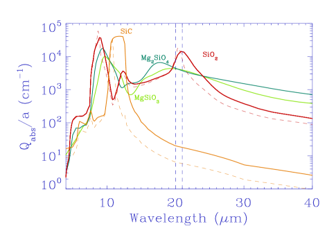
Figure 15: Optical constants for spherical silicate dust grains relevant for this work, including spherical grains of SiO₂ (red dotted line), SiC (orange dotted line), MgSiO₃ (green), and Mg₂SiO₄ (dark green). The continuous distribution of ellipsoidal (CDE) models for SiO₂ (red solid line) and SiC (orange solid line) are also shown (see the text for details).

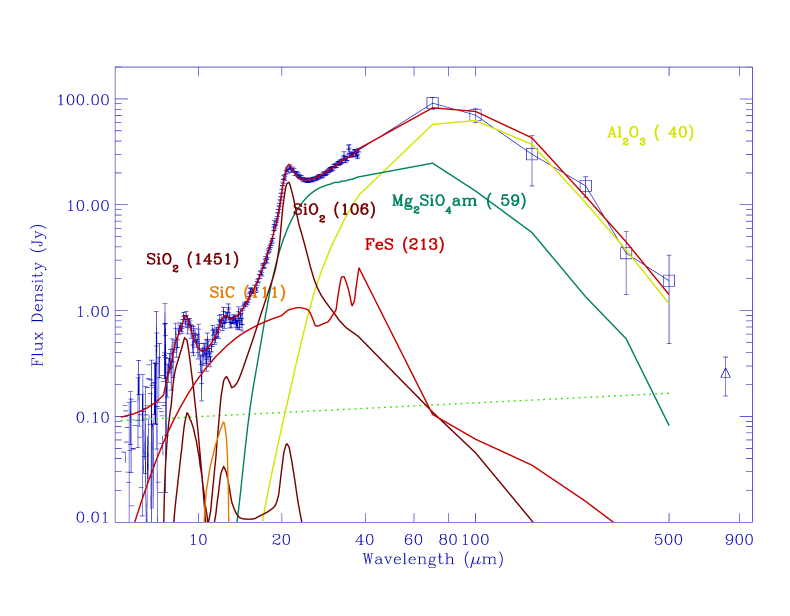
Figure 16: The spectral energy distribution of the SNR G54.1+0.3 from MIR - submm wavelengths (the broadband photometry from Table 3 and the IRS spectra are shown by blue data points) superposed on the dust fit of model A1 (see Table  4). The data and the total fit are shown in blue and thick red lines, respectively, and Herschel fluxes are marked with squares. The dust temperatures are shown in parentheses, and the dotted lines are from the second temperature components. Synchrotron continuum contribution (green dashed line) is estimated based on the radio fluxes . The 21$\mu$m and 11$\mu$m dust features are well produced by the CDE grain model of Silica and Silicon carbide (SiC), respectively. As well as the dust features and compositions required to fit the IRS spectrum of the SNR, we require a population of colder dust grains to explain the fluxes at wavelengths beyond 70 $\mu$m (see Section 4 for details). The different grain compositions required and fitting properties highlighted individually in this plot are listed in full in Table 4.

In an attempt to obtain a better fit to the SED of G54.1+0.3, we use the same SED fitting routine used for Cas A, but now try different grain compositions and different grain models. Specifically, we use the continuous distributions of ellipsoidals (CDE) grain model for SiO₂ (silica) and SiC (Silicon carbide) (Bohren & Huffman, 1985); the absorption efficiency for this grain species and others is shown in Figure 15. The first results of fitting using SiO₂ to reproduce the 21$\mu$m dust feature in Cas A were presented in conference proceeding (Rho et al., 2009a). The dust continuum is fit with the Planck function [B${}_{\nu}(T)$] multiplied by the absorption efficiency ($Q_{abs}$) for various dust compositions, varying the amplitude and temperature of each component. The optical constants of the grain species used in the calculation are the same as those of Hirashita et al. (2005), except for amorphous SiO₂ (Philipp, 1985), amorphous Al₂O₃ (Begemann et al., 1997) and we apply Mie theory (Bohren & Huffman, 1985) to calculate the absorption efficiencies, Q_abs, assuming the grains are small a$\leq$0.01 $\mu$m (Nozawa & Kozasa, 2013; Nozawa et al., 2010).

The dust mass of $i$-grain type is given by:

$$M_{dust,i}={F_{\nu}^{i}\,d^{2}\over{B_{\nu}(T_{d,i})\,\kappa_{i}}}={F_{\nu}^{i}d^{2}\over{B_{\nu}(T_{d,i})}}{4\,\rho_{i}\,a\over{3\,Q_{abs,i}}}$$

where $F_{\nu}^{i}$ is the flux from $i$-grain species, $d$ is the distance, $B_{\nu}$ is the Planck function, $\rho_{i}$ is the bulk density, and $a$ is the dust particle size. We fit the flux density for each spectral type using scale factors $C_{i}$ for each grain type $i$, such that F${}_{\nu}^{i}$ = $\Sigma_{i}\,C_{i}\,B_{\nu}\,Q_{abs,i}/a$, where Q($\lambda$, a) are calculated using Mie theory Bohren & Huffman (1985) and assuming a relatively small grain size a = 0.01 $\mu$m (Nozawa & Kozasa, 2013). Note that the calculated values of $Q_{abs}/a$ are independent of the grain size (a) for a $<<$0.1 $\mu$m at these wavelengths (i.e. as long as 2$\pi|m|a/\lambda$ $<<$1 where $m$ is the complex refractive index). Thus the derived scale factor C_i as well as the estimated dust mass (see Section 4.4) are independent of the radius of the dust. We applied this technique in our previous papers by Rho et al. (2009c); Arendt et al. (2014); Rho et al. (2008). The dust compositions of the best fits are summarized in Table 4.

We have quantified the goodness of fit ($\chi^{2}$) for the models using the mpfit IDL routine (Markwardt, 2009), though we note that there are degeneracies between the many different grain species that can fit the SED. The different models we tried with different grain compositions are described in full in Table 4. Note that the goodness of fit may depend on initial selection of grain composition.

Figure 17: Cas A spectral fitting using the Model A1 (Table 4), the same model as that of G54.1+0.3 to the Spitzer SED of Cas A from Rho et al. (2008). The model includes using the continuous distribution of ellipsoidal models instead of spherical grains for SiO₂ and SiC, which fairly well reproduce the 21$\mu$m and 11$\mu$m dust features, respectively.

4.1 Silica for 21$\mu$m dust and Silicon Carbide for 11$\mu$m dust features

Rho et al. (2008) fitted the IRS spectra and 21$\mu$m dust peak feature using a combination of grains that included SiO₂ (silica), Mg protosilicates, and FeO grains (their so-called Model A). However, Rho et al. (2008) noted that the 21$\mu$m feature was not perfectly reproduced with this model as shown in Figure 3 of their paper. Here we attempt to do a similar analysis for G54.1+0.3. We first performed spectral fitting of the 21$\mu$m-peak dust using the CDE grain model of SiO₂ and spherical model for MgSiO₃. The comparison of absorption coefficient between the spherical and CDE grain model in Figure 15 show that the SiO₂ and SiC CDE features are smoother, broader feature than those of spherical grain models. Here we find that the 21 $\mu$m peak dust for spectra of G54.1+0.3 is reasonably well fit by SiO₂ in Figure 16 without requiring Mg proto-silicates nor FeO in contrast to the original Cas A study. In addition, the newly identified 11-12.5$\mu$m feature seen here (Figure 10) can be fit with the SiC CDE grain model.

For a SiC grain of a given size "a" and a given 21$\mu$m feature strength ($Q_{abs}$/$a$), Jiang et al. (2005) calculate its equilibrium temperature and its emission spectrum to generate both dust feature at 11.3 and 21$\mu$m. However, the required strength for the 21$\mu$m feature is stronger than that for the 11.3 $\mu$m feature of SiC. Because the low-res spectrum covered an additional wavelength coverage at 5-10 $\mu$m which include the 9$\mu$m dust feature (see Figure 11), we used the low-res IRS spectrum together with Herschel photometry data for dust spectral fittings.

After we fit the CDE models of SiO₂ and SiC to reproduce the 21$\mu$m and 11$\mu$m dust features obtained in the low-res spectra of G54.1+0.3, we incorporate other grain compositions based on Model A from Rho et al. (2008) including amorphous FeS (150 K) and Mg₂SiO₄ (58 K) to account for the emission between 5-30$\mu$m, and Al₂O₃ to reproduce the spectra beween 30-500$\mu$m. We also include grains of SiO₂ at high temperature (300 K) to account for the emission feature around 9.8$\mu$m, but this component is added to mimic IR emission from stochastic heating (e.g. Rho et al. 2008, 2009c; Lagage et al. 1996). This model is shown in Figure 16 (Model A1); the fit produces a reduced $\chi^{2}$ of 3.7 and yields a total dust mass for the SNR of 0.16 M_⊙ (Table 4).

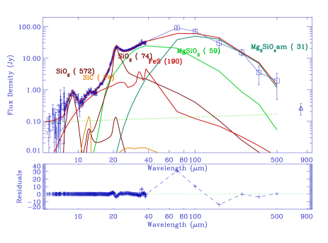
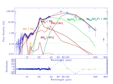
Figure 18: Spectral energy distribution of G54.1+0.3 superposed on the dust fit of a warm dust component made of MgSiO₃, with cold dust of Mg₂SiO₄ (Top: Model A2) and of Mg_2.3SiO₄ using its Q_abs at 30 K (Bottom: model A2F1), respectively. Silicate dust using a temperature-dependent (30 K) Q_abs produced a smaller dust mass (see Table 4).

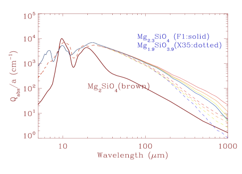
Figure 19: Optical constants for temperature dependent CDE models Mg_2.3SiO₄ (F1) and Mg_1.9SiO_3.9 (X35) (Demyk et al. 2013; Coupeaud et al. 2011) are compared with Mg₂SiO₄. For each sample of F1 and X35, the spectra are measured for a grain temperature of 300 K (red), 200 K (orange), 100 K (light green) and 30 K (blue).

As Model A1 is a good fit to G54.1+0.3, we next determine if this updated combination of grain compositions can also provide a better fit to the Cas A spectra compared to Rho et al. (2008). Figure 17 shows that indeed the CDE SiO₂ and SiC grains provide a better fit for the 21$\mu$m and 11$\mu$m dust features of Cas A, removing the residual seen in the IR in the earlier study. We note however that the IRS spectral coverage for G54.1+0.3 is limited to the center and south-western shell, and full spectral coverage may reveal different nucleosynthetic layers like those in Cas A. Temim et al. (2017) fit the 21$\mu$m dust feature of G54.1+0.3 with Mg_0.7SiO_2.7 and stated that they could not fit the 21$\mu$m feature using SiO₂ grains. We note that the shape of absorption coefficient of SiO₂ (Figure 4 of Temim et al., 2017) is different from the one we used in Figure 15. Our fits with SiO₂ reproduced the 21$\mu$m dust feature very well and the theoretical models (Nozawa et al., 2003; Bianchi & Schneider, 2007; Cherchneff & Dwek, 2010) predict production of silica in SN ejecta, and laboratory measurement (Haenecour et al., 2013) discovered two SiO₂ grains that are characterized by and originated from Type II SN ejecta.

Table 4: Dust Spectral fitting Results and Estimated Dust Mass. ^a - The 11$\mu$m dust feature includes a contribution from both SiC and hot dust composed of SiO₂. ^b - The three best solutions are in bold. $c$ - $\Delta$$\chi^{2}$ in the parenthesis is the reduced $\chi^{2}$ using statistical errors as weights. ^d - The number in the parenthesis is the dust temperature yielded from the spectral fitting for G54.1+0.3. Temperatures greater than $\sim$1800 K is from stocastic heating of the grains.

Modela	$\Delta\chi^{2}$	Dust Features		Dust components			Dust
	($\chi^{2}$/dof)	21$\mu$m	11$\mu$ma	Warm dust I	II [mass]	Cool dust	mass
		(K)	(K)	(K)	II (K) [M⊙]	(K) [M⊙]	(M⊙)
A1b	3.70 (1.44c)	SiO2 (106, 1450d)	SiC (110)	FeS (213)	Mg2SiO4 (59) [0.026]	Al2O3 (40) [0.13]	0.16
		($\pm$5, $\pm$1400)	($\pm$5)	($\pm$5)	($\pm$1) [$\pm$0.004]	($\pm$2) [$\pm$ 0.03]	($\pm$0.04)
A2	3.64 (4.42)	SiO2 (75, 572)d	SiC (74)	FeS (190)	MgSiO3 (59) [0.019]	Mg2SiO4 (31) [0.879]	0.90
		($\pm$2, $\pm$5)	($\pm$2)	($\pm$3)	($\pm$1) [$\pm$0.003]	($\pm$2) [$\pm$0.250]	[$\pm$0.30]
A2F1	4.60 (5.10)	SiO2 (73, 571)) [0.0019]	SiC (74)	FeS (191)	MgSiO3 (59) [0.020]	Mg2.3SiO4(29) [0.147]	0.17
		($\pm$2, $\pm$5) [$\pm$0.0003]	($\pm$1)	($\pm$3)	($\pm$1) [$\pm$0.002]	($\pm$2) [$\pm$0.036]	($\pm$0.04)
A2X35	4.60 (5.32)	SiO2 (74, 571)) [0.0021]	SiC (74)	FeS (191)	MgSiO3 (59) [0.020]	Mg1.9SiO3.9(27) [0.334]	0.36
		($\pm$2, $\pm$5) [$\pm$0.0003]	($\pm$2)	($\pm$3)	($\pm$1) [$\pm$0.003]	($\pm$2) [$\pm$0.102]	($\pm$0.11)
A3	4.89 (6.81)	SiO2 (69, 200) [0.003]	SiC (141)	FeS (189)	MgSiO3 (59) [0.019]	Al2O3 (30) [0.326]	0.35
		($\pm$2, $\pm$11) [$\pm$0.0008]	($\pm$88	($\pm$4)	($\pm$1) [$\pm$0.0015]	($\pm$2) [$\pm$0.08]	($\pm$0.09)
A4	3.72 (1.06)	SiO2 (109, 2793) [8E-5]	SiC (137)	FeS (213)	Mg2SiO4 (58) [0.033]	carbon (39) [0.223]	0.26
		($\pm$3, $\pm$92) [$\pm$2E-5]	($\pm$84)	($\pm$4)	($\pm$2) [$\pm$0.004]	($\pm$1) [$\pm$0.049]	($\pm$0.05)
A5	3.96 (1.69)	SiO2 (110, 2621) [8E-5]	SiC (276)	FeS (203)	Mg2SiO4 (55) [0.054]	Fe3O4 (42) [0.022]	0.08
		($\pm$2, $\pm$89) [$\pm$1E-5]	($\pm$182)	($\pm$4)	($\pm$1) [$\pm$0.007]	($\pm$2) [$\pm$0.004]	($\pm$0.01)
B1	3.57 (1.30)	SiO2 (113, 2686) [9.4E-5]	SiC (102)	C (180)	Mg2SiO4 (62) [0.018]	Al2O3 (42) [0.118]	0.14
		($\pm$1, $\pm$1326) [2.8E-5]	($\pm$48)	($\pm$4)	($\pm$1) [$\pm$0.003]	($\pm$1) [$\pm$0.008]	($\pm$0.01)
B2	4.56 (3.62)	SiO2 (75, 557) [1.57E-3]	SiC (74) [8.0E-4]	C (156) [1.2E-5]	MgSiO3 (56) [0.021]	Mg2SiO4 (32) [0.830]	0.85
		($\pm$2, $\pm$4) [0.26E-3]	($\pm$1) [$\pm$0.5E-4]	($\pm$2) [0.1E-5]	($\pm$1) [$\pm$2.5E-3]	($\pm$2) [$\pm$0.195]	($\pm$0.20)
B3	4.36 (4.76)	SiO2 (76, 509) [1.45E-3]	SiC (65) [7.9E-3]	C (160)	MgSiO3 (59) [0.021]	Al2O3 (33) [0.276]	0.31
		($\pm$2, $\pm$75) [0.25E-3]	($\pm$1) [$\pm$0.3E-3]	($\pm$2)	($\pm$1) [$\pm$0.002]	($\pm$2) [$\pm$0.061]	($\pm$0.06)
B4	4.18 (3.17)	SiO2 (113, 2719) [7E-5]	SiC (483)	C (169)	Mg2SiO4 (54) [0.073]	Fe3O4 (44) [0.0089]	0.08
		($\pm$2, $\pm$87) [$\pm$1E-5]	($\pm$25)	($\pm$5)	($\pm$1) [$\pm$0.008]	($\pm$3) [$\pm$0.001]	($\pm$0.01)

4.2 Exploring other SED fitting models

Here we compare the effect of assuming different grain properties and grain compositions. The results from all the models tested in this Section are listed in Table 4, along with the grain compositions assumed, and the resultant dust temperatures and masses. Some of the model fits and their residuals are shown in Figures 18 and 20. The 21$\mu$m and 11$\mu$m dust features are well produced by the CDE grain model of silica and Silicon carbide (SiC), respectively. As well as the dust features and compositions required to fit the IRS spectrum of the SNR, we require a population of colder dust grains to explain the fluxes at wavelengths $>$ 70 $\mu$m (Section  4).

In Model A1, the fit is produced with MgSiO₃ as a warm dust component, Al₂O₃ as a cold dust componen and with SiO₂ to reproduce the 21$\mu$m feature. We fit the same Model A1 to the spectrum of Cas A. The fit shown in Figure 17 yielded a dust mass of 0.06 M_⊙, a 60% higher dust mass than that from Model B (see Table 1) by Rho et al. (2008). Further work can explore the dust mass using SiO₂ and also including the long-wavelength band Herschel data. In Model A2, we change the cool dust composition in Model A1 from Al₂O₃ to Mg₂SiO₄ and the warm dust from Mg₂SiO₄ to MgSiO₃ (see Table 4). The fit is poorer and generated a higher dust mass ($0.9\,M_{\odot}$). Next Model A3 uses MgSiO₃ (59 K) and Al₂O₃ (30 K) instead of Mg₂SiO₄ (59 K) and Al₂O₃ (40 K) resulting in a dust mass of $0.35\,M_{\odot}$. Again this is a poorer fit, with residuals at 40-100$\mu$m and 300-500$\mu$m.

Next we checked the effect of using temperature dependent dust absorption properties. Dupac et al. (2003) observed large variations of the spectral index ($\beta\sim 0.8-2.4$) for dust with a wide range of temperatures (11 to 80 K), and suggested that there is an intrinsic dependence of the dust spectral index on the temperature (T-$\beta$ anticorrelation). The reasons can be the change in grain sizes, chemical composition of the grains in different environments and due to quantum processes. Paradis et al. (2011) also showed the flattening of the observed dust SED at far IR wavelengths using DIRBE, Archeops and WMAP, this results in an increased emissivity. Furthermore, Demyk et al. (2013, 2017) and Coupeaud et al. (2011) suggested that the absorption coefficient of amorphous silicate grains decreases with the temperature and shows a complex shape with the wavelength depending on the micro structure of the materials. For wavelengths shorter than $\sim$ 500 $\mu$m the spectral index is in the range 1.6-2.3 whereas at longer wavelengths it changes and its value may be outside this range. To determine if grains with temperature-dependent absorption properties could fit the SED of G54.1+0.3, we used two datasets for grain compositions closest to Mg₂SiO₄: one corresponds to glassy grains Mg_1.9SiO_3.9 (“X35" sample) and the other corresponds to a more porous sample of composition Mg_2.3SiO₄ (with a slight Mg excess, “F1" sample). The spectra of these two analogues are different because the analogues differs in terms of structure at micro- (nano-) meter scale, of porosity, of chemical composition and homogeneity at small scale. Figure 19 shows the optical constants of these materials. The Q_abs depart from $\beta$=2 at $>$ 200$\mu$m as shown in Figure 19. When Q_abs decreases at low temperature, the emissivity is flatter, and the flux is higher than expected with $\beta=2$. Models A2F1 and A2X35 therefore include Mg_2.3SiO₄ and Mg_1.9SiO_3.9 at a temperature of 30 K instead of Mg₂SiO₄. Since Mg₂SiO₄ has lower Q_abs at long wavelengths, this could result in a higher dust mass for the SNR. The fits for these models (Table 4, Figure 18) were not as good as the model with cold dust grains of Mg₂SiO₄ (Model A2) or Al₂O₃ (Model A1). We note that Q_abs of Mg_2.3SiO₄ and Mg_1.9SiO_3.9 show a factor of a few higher than that of Mg₂SiO₄ above 40 $\mu$m; this likely resulted in the poorer fit to the data.

Although theoretical models of dust formation in SNe (Nozawa et al., 2003; Todini & Ferrara, 2001) predicted that FeS grains are produced in the ejecta, we do not detect the sharp 34$\mu$m dust feature in the spectra of G54.1+0.3 and Cas A. We therefore try models where we replace FeS with carbon dust (with featureless absorption coefficient). First we replace the cold dust with carbon in Model A4. This provides one of the best fits to the observed data ($\Delta\chi^{2}=3.7$) with a total dust mass of $0.26\,M_{\odot}$. We also refit Models A1, A2 and A3 using carbon dust as the warm component (Models B1, B2, and B3 - Table 4) but find that the quality of the fits are slightly worse than those using FeS (Figure 20).

In order to reduce the relatively large residuals at medium or long wavelengths, we also included additional warm or cold dust components using MgSiO₃ or Al₂O₃, but the fits were not improved. We have fitted with SiO₂ grains as a cool dust component and the fit produced a large amount of dust of $sim$2.75 M_⊙ (see Table 4). However, this dust mass of SiO₂ is a factor of two larger than the SiO₂ dust mass constraints predicted by nuclear synthesis and dust formation models (Nozawa et al., 2003; Cherchneff & Dwek, 2010; Sukhbold et al., 2016; Temim et al., 2017); the predicted maximum SiO₂ dust is about 1.3 M_⊙ for the largest possible progenitor mass of 35 M_⊙. Thus, this model is a non-physical model and we excluded this model from the total dust mass estimates. We attempted to fit the spectra with two components of cool dust with the first component being SiO₂, and the second component being Mg₂SiO₄, Al₂O₃, or carbon dust, but the new fittings were not successful; the fits were either statistically insignificant when we accounted for the errors, or the reduced $\chi^{2}$ were too large. This is likely due to lack of far-IR data points.

Table 4 shows a summary of dust spectral fitting. The individual fit includes 6 components: hot and warm silica components (with temperature ranges of 200-2700 K and 70-115 K), Silicon carbide, two warm dust components (with temperature ranges of 150-210 K and 54-60 K), and a cool dust component (with a temperature range of 27-44 K). We also included grains of SiO₂ at high temperature (300 K) to account for the emission feature around 9.0$\mu$m, which was added to mimic IR emission from stochastic heating (eg Lagage et al. 1996; Rho et al. 2008).

What did heat those dust grains$?$ For the case of Cas A, the dominant heating source is a reverse shock. Since the dust is heated in young SNRs by the reverse shock, it was easier to be detected than that in SNe where a reverse shock has not yet passed SN ejecta (see Section 5.2 for details). When the gas temperature reaches about 1200 K that was $\sim$400 days after the SN explosion, dust forms and continues to cool down for 3-5 years, the exact time scale and temperature depending on the grain composition (see Nozawa et al., 2003). The dust in SNe is too cool to be detected or it is hard to distinguish the cool dust in SN ejecta from SN light echoes.

Koo et al. (2008) showed a few OB stars in the field of the SNR G54.1+0.3. Temim et al. (2010, 2017) and Kim et al. (2013) suggested that they belong to the same Stellar Cluster as the progenitor of the SNR G54.1+0.3. Using near-IR spectroscopic observations, Kim et al. (2013) showed that the stars are O9 (17Msun) and a few early B stars, and suggested the progenitor of G54.1+0.3 to be Type IIP with a mass range of 8-20 M_⊙ ($<<$ 35M_⊙), so the progenitor is likely not a Wolf-Rayet star. Later O and early B type stars have temperatures of 37,000 K to 15,000 K. Herschel observations of such stars show a dust temperature of $\sim$ 60-80K, which contribute a small amount of the dust mass. Therefore, the OB stars may be the source of the warm dust temperature, but it is not clear if they are the heating source of the cold temperature component of the dust (20-40K) in the SNR. The analogy of G54.1+0.3 to the Crab Nebula discussed below may suggest that OB stars alone may not be unique heating sources of the dust in G54.1+0.3, although the possibility cannot be ruled out with current evidence.

For the Crab-like SNRs, the heating source is different because the evidence of forward shock is unclear and thus the reverse shock may have not developed (Hester, 2008). Since G54.1+0.3 is a Crab-like SNR, we examined the heating mechanism of the Crab Nebula. The pulsar wind nebula of the Crab Nebula emits synchrotron radiation, where electrons are spinning around the magnetic field. The existence of this shock driven by the synchrotron nebula is recognized by Rayleigh-Taylor fingers (Sankrit et al., 1998) who estimate a shock velocity of 230 km s^-1, labeling the shock as nonradiative. Numerical simulations of the expansion of the Crab Nebula invariably identify these observed arcs with material from a surrounding freely expanding remnant that has been compressed by the synchrotron-driven shock (Jun, 1998; Bucciantini et al., 2004). The wind shock thermalizes flow energy, accelerating electrons and positrons to energies as high as $\sim$10⁴ TeV.

The dominant heating source for the dust in the Crab Nebula is known to be synchrotron radiation (i.e. nonthernal radiation field) in the pulsar wind nebula that depends on the luminosity of the synchrotron radiation (Davidson, 1973; Dwek & Werner, 1981; Dwek & Smith, 1996; Temim & Dwek, 2013). Grains are also heated by collisions between the electrons and the gas in the filaments, but this heating is suggested to be insignificant in the Crab-like SNRs (Hester, 2008; Dwek & Werner, 1981; Temim & Dwek, 2013; Temim et al., 2012). We are suggesting the heating source of G54.1+0.3 is similar to that of the Crab Nebula, dominant heating being photoionization from synchrotron emission, synchrotron-driven shock and possible contribution from collisional heating. Our results do not support the claim that the stellar members of the SN progenitor’s cluster in G54.1+0.3 are the primary heating sources for the SN dust by Temim et al. (2017) because we do not detect excess of the temperature and dust mass at the position of stars (see Figure 14). The blob with the high temperature on the western shell (Figure 14a) coincides with the bright blob on the western shell in the 24$\mu$m image and does not coincide with stars in the cluster. The heating source of G54.1+0.3, which is responsible for the warm and cool grains we observe, is likely photoionization from the synchrotron emission in the G54.1+0.3’s pulsar wind nebula.

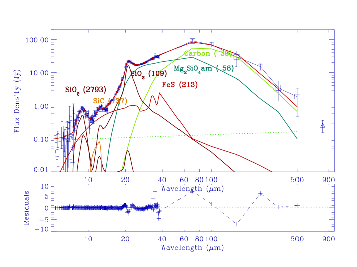
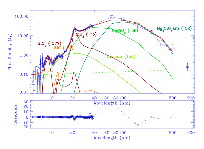
Figure 20: Spectral energy distribution of G54.1+0.3 superposed on the dust fit of Top: Model A4, assuming the cool dust component is made out of carbon and this fit produces the best fit after accounting the errors as weights. Bottom: The dust fit of Model B2; this is the same as Model A2 except that carbon is assumed for the warm dust instead of FeS. The set of Model A with the warm dust of FeS produces a better dust fit than those of Model B with the warm dust of carbon.

5 Discussion

5.1 Pre-solar Grains of Silica Produced in Supernovae

Pre-solar grains are those formed before our Solar system in ancient stellar outflows or ISM or supernovae and they are recognized by their highly unusual isotopic compositions relative to all other materials (e.g. Zinner 2013). Silicon carbide (SiC) is the best-studied type of presolar grain and has been suggested to be formed in supernovae. Another well-known pre-solar grain is corundum (Al₂O₃), low-density graphite (e.g. carbon grains), amorphous silicates, forsterite and enstatite, and corundum (Messenger et al., 2006). Some isotopic anomalies of heavy elements, especially ¹⁶O-enrichments, in meteorites have been attributed to the dust that had condensed deep within expanding supernovae (Clayton & Nittler, 2004). The existence of isotopic anomalies in a major element within meteoritic solids provided a decade of motivation for the search for supernova stardust. Meteoritic studies have shown that some types of presolar grains condense in the dense, warm stellar winds of evolved stars but other types of presolar grains (such as SiC-X grains) condenses in supernova explosions (Clayton & Nittler, 2004). Mantles on grains in molecular clouds are vaporized as stars form in the clouds. A small fraction of dust survives planet formation without alteration, protected inside asteroids.

We show that 10-13$\mu$m dust feature observed in G54.1+0.3 and Cas A are attributed to Silicon carbide using two methods. We showed that spectral fitting with the CDE model of SiC can reproduce the 11$\mu$m dust feature again both for G54.1+0.3 and Cas A (see Figures 16, 17, 18 and 20). We suggest that SiC is responsible for the broad dust bump between 10-13$\mu$m whereas the PAH emission is responsible for the features at 11.0, 11.2 and 12.7$\mu$m (see Section 3.2.3).

Table 5: Summary of Dust Mass from Young Supernova Remnants. ^a - The upper limit of warm dust mass estimated using Spitzer data only. Publications are: (1) Matsuura et al. (2015); (2) De Looze et al. (2017); (3) Rho et al. (2008); (4) Gomez et al. (2012); (5) Owen & Barlow (2015); (6) Temim et al. (2012); this paper (^bsee the text for detailed discussion and comparison with Temim et al. 2017); (7) Temim et al. (2010).

SNR	dust mass [Spitzera]	dust temperature	dominant	progenitor	ref.
	(M⊙)	K	dust type	(M⊙)
SN1987A	0.4-0.7 [$>$1.3$\times$10-3]	17-23	carbon	18-20: Type II	1
Cas A	0.3-0.5 [0.054]	30	silicate	25-30: Type II/Ib	2, 3
Crab Nebula	0.1-0.54 [0.012]	25-36	carbon	10-12: Type II	4, 5, 6
G54.1+0.3	0.08-0.9 [0.02]	27-44	silicate	15-35: Type II	this paperb, 7

New presolar phases, such as SiO₂ have been identified with the Auger spectroscopy to characterize the elemental compositions of pre-solar silicate and oxide grains (Nguyen et al., 2010). They all exhibit enrichments in ¹⁷O relative to solar, indicating origins in the envelopes of AGB stars (Messenger et al., 2006). We showed that the 21$\mu$m dust feature in G54.1+0.3 and Cas A can be reproduced with the CDE model of amorphous silica (SiO₂). Theoretical models by Nozawa et al. (2003) predicted silica dust grains in supernova ejecta as well as other silicate dust such as enstatite (MgSiO₃) and forsterite (Mg₂SiO₄) as our spectral fitting also supports. Following Schneider et al. (2004), Bianchi & Schneider (2007) have added the formation of SiO₂ grains. We presented the first results of fitting using SiO₂ to reproduce the 21$\mu$m dust feature in Cas A in conference proceeding (Rho et al., 2009a). Inspired from that, Haenecour et al. (2013) searched SiO₂ from the primitive carbonaceous chondrites LaPaZ 031117 and Grove Mountains 021710 from meteorites, and they discovered two SiO₂ grains that are characterized by moderate enrichments in ¹⁸O relative to solar and originated in Type II supernova ejecta. This proves that SiO₂ is also pre-solar grains which are originated from supernovae. The discovery of these two silica grains in laboratory provides support that the silica dust which re-produces the 21$\mu$m dust feature in the young SNR G54.1+0.3 and Cas A. Arendt et al. (2014) suggested that magnesium silicates (particularly Mg_0.7SiO_2.7 have peaks that are in roughly the right locations, but their shapes are not a good match to the IRS data of Cas A, although two-composition fits help to improve the fits. This particular silicates are not predicted by theoretical models of dust in SN ejecta and our SiO₂ produces a better fit than that. Note that our Q_abs of SiO₂ is different from that in Arendt et al. (2014).

The dust mass of silica depends on the progenitor mass, and different theoretical models predict different amounts of dust mass. The progenitor of G54.1+0.3 has a large range between 15-35 M_⊙ (see Table 5). The observed SiO₂ dust masses range from 10^-5 to 2$\times$10^-3 M_⊙. Theoretical models (Nozawa et al., 2003) predicted that for the unmixed case the dust mass of SiO₂ is 0.02 - 0.2 M_⊙ ( 5% - 12% of the total dust mass), and for mixed case the dust mass of SiO₂ is 0.6 - 1.3 M_⊙ (70% - 50% of the total mass). The other dominant dust mass is predicted to be from Mg₂SiO₄. Cherchneff & Dwek (2010) predicted that the dust mass of SiO₂ is 67% (about 0.1 M_⊙) of the total dust mass for the no depletion case, while very small percent of SiO₂ is formed for the Mg/Fe depleted case. Sarangi & Cherchneff (2013) suggest a small amount of SiO₂, one order of 10^-5 M_⊙ as we observed for most of our spectral models. In order to accurately characterize a dozen dust species that are predicted by the theoretical models, a higher number of far-IR data points or far-IR spectroscopic data are required. Theoretical models of small grids in the progenitor mass and other physical parameters that determine the dust mass will also be helpful.

5.2 The dust mass in supernova ejecta and its implication to the dust in the early Universe

The dust mass we estimated from G54.1+0.3 is 0.08-0.90$\,M_{\odot}$ (see Table 4) depending on the grain composition, which is comparable to predicted masses from theoretical models. The dust mass estimate of G54.1+0.3 can be more accurate than that of Cas A because of the following two reasons; (1) the foreground ISM contribution is less obvious than that of Cas A (Barlow et al., 2010) in far-IR emission as shown in Figure 3, and (2) the dust destruction due to the forward or reverse shock is less significant because the SNR G54.1+0.3 is a Crab-like SNR. G54.1+0.3 and Cas A have typical foreground emission of 0.08 and 0.32 Jy (9^′′pixel)^-1 at 160$\mu$m, and 0.3 and 0.55 Jy beam^-1 at 250$\mu$m, respectively. The surface brightness of the foreground emission in vicinity of G54.1+0.3 is $\sim$20-30 percent of the SNR brightness, whereas the typical brightness of foreground emission near Cas A is $\sim$90 - 115 percent of the Cas A brightness. Most importantly, the filamentary cirrus structures continue to be present across the SNR Cas A in the Herschel images (see Figure 1 of Barlow et al., 2010), while such cirrus structures are not obvious toward G54.1+0.3 (see Figures 3 and 4). The statistical uncertainties of dust temperatures and masses for each spectral fitting results are given in Table 4. The uncertainty of dust mass ranges between 7-35 percent.

Our estimated dust mass is somewhat lower (0.07-1.2 M_⊙ after accounting for the errors) than that (1.1$\pm$0.8 M_⊙) obtained by Temim et al. (2017). Considering completely independent methods, this is a reasonable agreement since the systematic errors could be this large caused by different grain compositions, absorption coefficiencies used and the flux measurements of Herschel due to large background variations.

In Table 4, the dust mass of 0.08-0.90$\,M_{\odot}$ primarily comes from the cool dust component ($>$90%), and the warm dust contributes to the dust mass less than 10% except the case of of Fe₃O₄ as a cool dust (model A5 and B4). Another noticeable conclusion is when we use Mg₂SiO₄ as a cool component, the fitting (Models A1 and B2) gives higher dust masses than the other models. Bianchi & Schneider (2007) show that large amounts (0.1 M_⊙) of cool dust (T $\sim$ 40 K) can be present which is similar to what we observed within a factor of 3, and for the case of olivine Mg₂SiO₄ as a cool dust component we observed a large dust mass (up to 0.88 M_⊙).

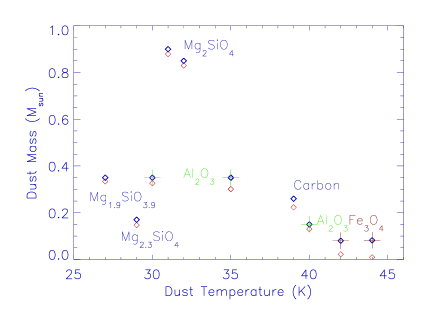
Figure 21: The derived dust mass for dust grains at different dust temperatures and assumed grain compositions. The total dust mass and the dust mass of the cool component are marked as diamonds in blue and red, respectively.

We examined the correlation between the derived dust mass and the fitted dust temperature of the cool component. There is an expectation that dust mass is higher when the dust temperature is lower as the cool dust dominates its dust mass as shown in Table 4. Gall et al. (2011) also shows this correlation in young SNe. Figure 21 shows the distribution of dust temperature versus mass for the cool dust component for G54.1+0.3 given the compositions assumed in this work. The dust mass is inversely proportional to the Planck function which is a function of temperature as shown in the equation in Section 4. The trend is observed in Figure 21 when we exclude Mg₂SiO₄. The dust mass depends on not only the temperature but also the density and absorption coefficient of the grain composition. The cold grains dominate the dust mass as shown in Table 4. However, for some cases, the dust mass of warm dust was higher than that of cool dust (see the case of Model A5) where the warm dust reproduces the large portion of continuum and has low Q_abs compared with those of other grains (see Fig. 19). The total mass of dust we derive here for a range of grain compositions is between 0.08-0.9 M_⊙ including temperature-dependent silicate grains. The one exception is when we assume grains composed of forsterite (Mg₂SiO₄) which yields a higher dust mass than other models. Our results show that the grain composition is also an important factor as well as the temperature to determine the total dust mass (as well as the cool dust temperature).

Whether some of the dust formed in the ejecta will survive is a major unresolved issue. The lifetimes of the major dust materials (i.e. carbon and silicates) against the rate of destruction by SN shock waves appear to be too short compared to the time-scales for the formation of new dust (Jones et al., 1994). Recent simulations by Slavin et al. (2015) shows that the dust destruction timescales are increased by a factor of 2-6 times compared to those of Jones et al. (1996) when accounting for the thermal history of a shocked gas and longer silicate grain destruction timescale. Nath et al. (2008) find that a fraction of the dust mass (1%- 20% for silicates and graphites) can be sputtered by reverse shocks, the fraction varying with the size of ejecta knots, the grain size distribution and the steepness of the density profile of the ejecta mass. Silvia et al. (2010) find that for high ejecta densities, the percentage of dust that survives is strongly dependent on the relative velocity between the clump and the reverse shock, causing up to 50% more destruction for the highest velocity shock. The rates of dust destruction therefore depends on the pre-shock density, progenitor mass, shock speed and so on. At least 2-20% of dust is survived behind the reverse shock (Bianchi & Schneider, 2007; Micelotta et al., 2016) where knots can be as dense as 10⁸ cm^-3 (based on CO observations for Cas A Rho et al., 2009b; Rho et al., 2012b). For G54.1+0.3, dust destruction by a forward shock may be less critical, since the evidence of strong forward shock has not been observed in the Crab-like SNRs (Hester, 2008).

Our observations of G54.1+0.3 implies that 0.08-0.9 M_⊙ of dust is formed in the ejecta with cool temperatures ranging from 27-44 K. This mass is consistent with the predicted dust mass from the theoretical models of dust formation in SN ejecta (Nozawa et al., 2003; Todini & Ferrara, 2001; Bianchi & Schneider, 2007). The estimated dust mass from the G54.1+0.3 implies that SNe are a significant source of dust in the early Universe. Table 5 compares the dust masses observed with Spitzer alone and a combination of Spitzer and Herschel observations. The dust masses observed with Herschel are an order of magnitude larger than those previously measured in these remnants using Spitzer, and are two orders of magnitude higher than those observed in young SNe (Kotak et al., 2006; Gall et al., 2011). As with SN1987A, Cas A and the Crab Nebula (see Table 5), we find that the mass of dust in the G54.1+0.3 SNR is very different based on SED fitting with and without adding the FIR-submm regime. Spectral fitting including the long wavelength SED in Figure 16 requires a significant amount of dust at lower temperatures. Thus, this work adds to the growing evidence that core-collapse SNe are forming large quantities of dust.

Future JWST observations of SNe will help to resolve if the dust observed in SNe is from ejecta, dense shell from stellar wind, or from light echos, and will allow us to observe dust formation of different types of dust from 300 - 800 days after the explosion.

6 Conclusion

1. We report the detection of far-infrared and submillimeter emission from the Crab-like SNR G54.1+0.3 using SHARC-II, LABOCA and Herschel observations (70-500$\mu$m).

2. Using Spitzer archival IRS, IRAC, and MIPS data, we detected a 21$\mu$m dust feature in G54.1+0.3 remarkably similar to that seen in Cas A. As in Cas A, this 21$\mu$m dust feature is coincident with the ejecta line emission as traced by [Ar II]. SED fitting suggests that the 21$\mu$m feature is composed of SiO₂ grains. The 21$\mu$m feature in the SNRs G54.1+0.3 and Cas A is offset by $\sim$1$\mu$m from the dust feature (peaking at 20.3$\mu$m) in the PPNe or carbon stars, and neither SNR has a broad dust bump at 30$\mu$m which is seen in the PPNe. The 21$\mu$m dust feature, therefore, seems to be unique to Cas A and G54.1+0.3 to date.

3. We suggest that the 21$\mu$m dust features in G54.1+0.3 and Cas A are attributed to the presolar grains of SiO₂. We raise a possibility that the 11$\mu$m dust features may come from the pre-solar grain of SiC with a combination of PAH contribution.

4. We reveal a cold dust component (27-44 K) coincident with the SNR with a total dust mass of $0.08-0.9\,M_{\odot}$ depending on the grain composition within the ejecta. If the FIR and submm emission is indeed dust formed in the ejecta, this makes G54.1+0.3 one of only four SNRs where cold dust is detected. The amount of dust mass observed from the SNR G54.1+0.3 suggests that SNe are a significant source of dust in the early Universe.

We thank anonymous referee for insightful comments, which helped to improve the paper. JR acknowledges support from NASA ADAP grant (NNX12AG97G which was rolled over from NNX10AQ84G) for the study of SN dust. HLG acknowledges support from the European Research Council (ERC) in the form of Consolidator Grant CosmicDust (ERC-2014-CoG-647939, PI H L Gomez). We thanks Karine Demyk for providing absorption coefficients prior to her publication, Mikako Matsuura for information and discussion about SN1987A and dust in SNRs, and William Reach for helping calculation of mineral properties. JR thanks Achim Tappe to reduce the IRS spectra for proto-planetary nebulae.

References

- Acciari et al. (2010) Acciari V. A., et al., 2010, ApJ, 719, L69
- Andrews et al. (2011) Andrews J. E., et al., 2011, AJ, 142, 45
- Arendt et al. (2014) Arendt R. G., Dwek E., Kober G., Rho J., Hwang U., 2014, ApJ, 786, 55
- Barlow et al. (2010) Barlow M. J., et al., 2010, A&A, 518, L138
- Begemann et al. (1997) Begemann B., Dorschner J., Henning T., Mutschke H., Gürtler J., Kömpe C., Nass R., 1997, ApJ, 476, 199
- Benjamin et al. (2003) Benjamin R. A., et al., 2003, PASP, 115, 953
- Bianchi & Schneider (2007) Bianchi S., Schneider R., 2007, MNRAS, 378, 973
- Bocchino et al. (2010) Bocchino F., Bandiera R., Gelfand J., 2010, A&A, 520, A71
- Bocchio et al. (2016) Bocchio M., Marassi S., Schneider R., Bianchi S., Limongi M., Chieffi A., 2016, A&A, 587, A157
- Boersma et al. (2013) Boersma C., Bregman J. D., Allamandola L. J., 2013, ApJ, 769, 117
- Bohren & Huffman (1985) Bohren C. F., Huffman D. R., 1985, Absorption and Scattering of Light by Small Particles. New York: Wiley
- Bucciantini et al. (2004) Bucciantini N., Bandiera R., Blondin J. M., Amato E., Del Zanna L., 2004, A&A, 422, 609
- Cerrigone et al. (2011) Cerrigone L., Trigilio C., Umana G., Buemi C. S., Leto P., 2011, MNRAS, 412, 1137
- Cherchneff & Dwek (2010) Cherchneff I., Dwek E., 2010, ApJ, 713, 1
- Clark et al. (2016) Clark C. J. R., Schofield S. P., Gomez H. L., Davies J. I., 2016, MNRAS, 459, 1646
- Clayton & Nittler (2004) Clayton D. D., Nittler L. R., 2004, ARA&A, 42, 39
- Coupeaud et al. (2011) Coupeaud A., et al., 2011, A&A, 535, A124
- Davidson (1973) Davidson K., 1973, ApJ, 186, 223
- De Looze et al. (2017) De Looze I., Barlow M. J., Swinyard B. M., Rho J., Gomez H. L., Matsuura M., Wesson R., 2017, MNRAS, 465, 3309
- Demyk et al. (2013) Demyk K., et al., 2013, in Proceedings of The Life Cycle of Dust in the Universe: Observations, Theory, and Laboratory Experiments (LCDU2013). 18-22 November, 2013. Taipei, Taiwan. Editors: Anja Andersen, Maarten Baes, Haley Gomez, Ciska Kemper, Darach Watson. Online at http://pos.sissa.it/cgi-bin/reader/conf.cgi?confid=207, id.44. p. 44
- Demyk et al. (2017) Demyk K., et al., 2017, A&A, 600, A123
- Dunne et al. (2003) Dunne L., Eales S., Ivison R., Morgan H., Edmunds M., 2003, Nature, 424, 285
- Dunne et al. (2009) Dunne L., et al., 2009, MNRAS, 394, 1307
- Dupac et al. (2003) Dupac X., et al., 2003, A&A, 404, L11
- Dwek & Smith (1996) Dwek E., Smith R. K., 1996, ApJ, 459, 686
- Dwek & Werner (1981) Dwek E., Werner M. W., 1981, ApJ, 248, 138
- Dwek et al. (2007) Dwek E., Galliano F., Jones A. P., 2007, ApJ, 662, 927
- Gall et al. (2011) Gall C., Hjorth J., Andersen A. C., 2011, A&ARv, 19, 43
- Gall et al. (2014) Gall C., et al., 2014, Nature, 511, 326
- Gomez (2013) Gomez H., 2013, in Proceedings of The Life Cycle of Dust in the Universe: Observations, Theory, and Laboratory Experiments (LCDU2013). 18-22 November, 2013. Taipei, Taiwan.
- Gomez (2014) Gomez H., 2014, Nature, 511, 296
- Gomez et al. (2012a) Gomez H. L., et al., 2012a, MNRAS, 420, 3557
- Gomez et al. (2012b) Gomez H. L., et al., 2012b, ApJ, 760, 96
- Gomez et al. (2012c) Gomez H. L., et al., 2012c, ApJ, 760, 96
- Green (1985) Green D. A., 1985, MNRAS, 216, 691
- Griffin et al. (2010) Griffin M. J., et al., 2010, A&A, 518, L3
- Güsten et al. (2006) Güsten R., Nyman L. Å., Schilke P., Menten K., Cesarsky C., Booth R., 2006, A&A, 454, L13
- Haenecour et al. (2013) Haenecour P., Zhao X., Floss C., Lin Y., Zinner E., 2013, ApJ, 768, L17
- Hester (2008) Hester J. J., 2008, ARA&A, 46, 127
- Hirashita et al. (2005) Hirashita H., Nozawa T., Kozasa T., Ishii T. T., Takeuchi T. T., 2005, MNRAS, 357, 1077
- Hony et al. (2001) Hony S., Van Kerckhoven C., Peeters E., Tielens A. G. G. M., Hudgins D. M., Allamandola L. J., 2001, A&A, 370, 1030
- Hudgins & Allamandola (1999) Hudgins D. M., Allamandola L. J., 1999, ApJ, 516, L41
- Indebetouw et al. (2014) Indebetouw R., et al., 2014, ApJ, 782, L2
- Jiang et al. (2005) Jiang B. W., Zhang K., Li A., 2005, ApJ, 630, L77
- Jones et al. (1994) Jones A. P., Tielens A. G. G. M., Hollenbach D. J., McKee C. F., 1994, ApJ, 433, 797
- Jones et al. (1996) Jones A. P., Tielens A. G. G. M., Hollenbach D. J., 1996, ApJ, 469, 740
- Jun (1998) Jun B.-I., 1998, ApJ, 499, 282
- Kim et al. (2013) Kim H.-J., Koo B.-C., Moon D.-S., 2013, ApJ, 774, 5
- Koo et al. (2008) Koo B.-C., et al., 2008, ApJ, 673, L147
- Kotak et al. (2006) Kotak R., et al., 2006, ApJ, 651, L117
- Kotak et al. (2009) Kotak R., et al., 2009, ApJ, 704, 306
- Kovács et al. (2006) Kovács A., Chapman S. C., Dowell C. D., Blain A. W., Ivison R. J., Smail I., Phillips T. G., 2006, ApJ, 650, 592
- Krause et al. (2004) Krause O., Birkmann S. M., Rieke G. H., Lemke D., Klaas U., Hines D. C., Gordon K. D., 2004, Nature, 432, 596
- Kwok et al. (1989) Kwok S., Volk K. M., Hrivnak B. J., 1989, ApJ, 345, L51
- Lagage et al. (1996) Lagage P. O., Claret A., Ballet J., Boulanger F., Cesarsky C. J., Cesarsky D., Fransson C., Pollock A., 1996, A&A, 315, L273
- Lang et al. (2010) Lang C. C., Goss W. M., Cyganowski C., Clubb K. I., 2010, ApJS, 191, 275
- Leahy et al. (2008) Leahy D. A., Tian W., Wang Q. D., 2008, AJ, 136, 1477
- Lee et al. (2012) Lee J.-W., Koo B.-C., Lee J.-E., 2012, Journal of Korean Astronomical Society, 45, 117
- Li et al. (2013) Li A., Liu J. M., Jiang B. W., 2013, ApJ, 777, 111
- Loh et al. (2011) Loh E. D., Baldwin J. A., Curtis Z. K., Ferland G. J., O’Dell C. R., Fabian A. C., Salomé P., 2011, ApJS, 194, 30
- Lu et al. (2002) Lu F. J., Wang Q. D., Aschenbach B., Durouchoux P., Song L. M., 2002, ApJ, 568, L49
- Maiolino et al. (2004) Maiolino R., Schneider R., Oliva E., Bianchi S., Ferrara A., Mannucci F., Pedani M., Roca Sogorb M., 2004, Nature, 431, 533
- Markwardt (2009) Markwardt C. B., 2009, in Bohlender D. A., Durand D., Dowler P., eds, Astronomical Society of the Pacific Conference Series Vol. 411, Astronomical Data Analysis Software and Systems XVIII. p. 251 (arXiv:0902.2850)
- Matsuura et al. (2011) Matsuura M., et al., 2011, Science, 333, 1258
- Matsuura et al. (2014) Matsuura M., et al., 2014, MNRAS, 439, 1472
- Matsuura et al. (2015) Matsuura M., et al., 2015, ApJ, 800, 50
- Mattsson (2015) Mattsson L., 2015, preprint, (arXiv:1505.04758)
- Mattsson et al. (2014) Mattsson L., et al., 2014, MNRAS, 444, 797
- McCray & Fransson (2016) McCray R., Fransson C., 2016, ARA&A, 54, 19
- McKee et al. (1987) McKee C. F., Hollenbach D. J., Seab G. C., Tielens A. G. G. M., 1987, ApJ, 318, 674
- Meikle et al. (2011) Meikle W. P. S., et al., 2011, ApJ, 732, 109
- Messenger et al. (2006) Messenger S., Sandford S., Brownlee D., 2006, The Population of Starting Materials Available for Solar System Construction. pp 187–208
- Micelotta et al. (2016) Micelotta E. R., Dwek E., Slavin J. D., 2016, A&A, 590, A65
- Michałowski (2015) Michałowski M. J., 2015, A&A, 577, A80
- Michałowski et al. (2010) Michałowski M., Hjorth J., Watson D., 2010, A&A, 514, A67
- Molinari et al. (2010) Molinari S., et al., 2010, PASP, 122, 314
- Morgan & Edmunds (2003) Morgan H. L., Edmunds M. G., 2003, MNRAS, 343, 427
- Nath et al. (2008) Nath B. B., Laskar T., Shull J. M., 2008, ApJ, 682, 1055
- Nguyen et al. (2010) Nguyen A. N., Nittler L. R., Stadermann F. J., Stroud R. M., Alexander C. M. O., 2010, ApJ, 719, 166
- Nguyen et al. (2016) Nguyen A. N., Keller L. P., Messenger S., 2016, ApJ, 818, 51
- Nozawa & Kozasa (2013) Nozawa T., Kozasa T., 2013, ApJ, 776, 24
- Nozawa et al. (2003) Nozawa T., Kozasa T., Umeda H., Maeda K., Nomoto K., 2003, ApJ, 598, 785
- Nozawa et al. (2010) Nozawa T., Kozasa T., Tominaga N., Maeda K., Umeda H., Nomoto K., Krause O., 2010, ApJ, 713, 356
- Ott (2010) Ott S., 2010, in Mizumoto Y., Morita K.-I., Ohishi M., eds, Astronomical Society of the Pacific Conference Series Vol. 434, Astronomical Data Analysis Software and Systems XIX. p. 139 (arXiv:1011.1209)
- Owen & Barlow (2015) Owen P. J., Barlow M. J., 2015, ApJ, 801, 141
- Paradis et al. (2011) Paradis D., Bernard J.-P., Mény C., Gromov V., 2011, A&A, 534, A118
- Peeters et al. (2017) Peeters E., Bauschlicher Jr. C. W., Allamandola L. J., Tielens A. G. G. M., Ricca A., Wolfire M. G., 2017, ApJ, 836, 198
- Philipp (1985) Philipp H., 1985, Handbook of Optical Constants of Solids, ed. E. D. Palik. San Diego: Academic Press
- Pilbratt et al. (2010) Pilbratt G. L., et al., 2010, A&A, 518, L1
- Planck Collaboration et al. (2011) Planck Collaboration et al., 2011, A&A, 536, A7
- Poglitsch et al. (2010) Poglitsch A., et al., 2010, A&A, 518, L2
- Reich et al. (1985) Reich W., Fuerst E., Altenhoff W. J., Reich P., Junkes N., 1985, A&A, 151, L10
- Rho et al. (2008) Rho J., et al., 2008, ApJ, 673, 271
- Rho et al. (2009a) Rho J., et al., 2009a, in Henning T., Grün E., Steinacker J., eds, Astronomical Society of the Pacific Conference Series Vol. 414, Cosmic Dust - Near and Far. p. 22 (arXiv:0901.1699)
- Rho et al. (2009b) Rho J., Jarrett T. H., Reach W. T., Gomez H., Andersen M., 2009b, ApJ, 693, L39
- Rho et al. (2009c) Rho J., Reach W. T., Tappe A., Hwang U., Slavin J. D., Kozasa T., Dunne L., 2009c, ApJ, 700, 579
- Rho et al. (2010) Rho J., Gomez H., Lagage P.-O., Boogert A., Reach W. T., Dowell D., 2010, in 38th COSPAR Scientific Assembly. p. 2
- Rho et al. (2012a) Rho J., Park S., Boogert A., Gomez H., Reach W., Dowell D., Lagage P., 2012a, in American Astronomical Society Meeting Abstracts #220. p. 431.01
- Rho et al. (2012b) Rho J., Onaka T., Cami J., Reach W. T., 2012b, ApJ, 747, L6
- Roussel (2013) Roussel H., 2013, PASP, 125, 1126
- Sandstrom et al. (2008) Sandstrom K., Bolatto A., Leroy A., Stanimirovic S., Simon J. D., Staveley-Smith L., Shah R., 2008, 381, 268
- Sankrit et al. (1998) Sankrit R., et al., 1998, ApJ, 504, 344
- Sarangi & Cherchneff (2013) Sarangi A., Cherchneff I., 2013, ApJ, 776, 107
- Schneider et al. (2004) Schneider R., Ferrara A., Salvaterra R., 2004, MNRAS, 351, 1379
- Schuller et al. (2009) Schuller F., et al., 2009, A&A, 504, 415
- Sibthorpe et al. (2010) Sibthorpe B., et al., 2010, ApJ, 719, 1553
- Silvia et al. (2010) Silvia D. W., Smith B. D., Shull J. M., 2010, ApJ, 715, 1575
- Siringo et al. (2009) Siringo G., et al., 2009, A&A, 497, 945
- Slavin et al. (2015) Slavin J. D., Dwek E., Jones A. P., 2015, ApJ, 803, 7
- Sloan et al. (2014) Sloan G. C., et al., 2014, ApJ, 791, 28
- Smith (2013) Smith N., 2013, MNRAS, 434, 102
- Smith et al. (2007) Smith J. D. T., et al., 2007, PASP, 119, 1133
- Smith et al. (2009) Smith J. D. T., Rudnick L., Delaney T., Rho J., Gomez H., Kozasa T., Reach W., Isensee K., 2009, ApJ, 693, 713
- Sugerman et al. (2006) Sugerman B. E. K., et al., 2006, Science, 313, 196
- Sukhbold et al. (2016) Sukhbold T., Ertl T., Woosley S. E., Brown J. M., Janka H.-T., 2016, ApJ, 821, 38
- Temim & Dwek (2013) Temim T., Dwek E., 2013, ApJ, 774, 8
- Temim et al. (2010) Temim T., Slane P., Reynolds S. P., Raymond J. C., Borkowski K. J., 2010, ApJ, 710, 309
- Temim et al. (2012) Temim T., Sonneborn G., Dwek E., Arendt R. G., Gehrz R. D., Slane P., Roellig T. L., 2012, ApJ, 753, 72
- Temim et al. (2017) Temim T., Dwek E., Arendt R. G., Borkowski K. J., Reynolds S. P., Slane P., Gelfand J. D., Raymond J. C., 2017, ApJ, 836, 129
- Todini & Ferrara (2001) Todini P., Ferrara A., 2001, MNRAS, 325, 726
- Valiante et al. (2009) Valiante R., Schneider R., Bianchi S., Andersen A. C., 2009, MNRAS, 397, 1661
- Velusamy & Becker (1988) Velusamy T., Becker R. H., 1988, AJ, 95, 1162
- Ventura et al. (2012) Ventura P., et al., 2012, MNRAS, 424, 2345
- Volk et al. (2011) Volk K., et al., 2011, ApJ, 735, 127
- Watson et al. (2015) Watson D., Christensen L., Knudsen K. K., Richard J., Gallazzi A., Michałowski M. J., 2015, Nature, 519, 327
- Wesson et al. (2015) Wesson R., Barlow M. J., Matsuura M., Ercolano B., 2015, MNRAS, 446, 2089
- Woosley & Weaver (1995) Woosley S. E., Weaver T. A., 1995, ApJS, 101, 181