Accurate Chemical Master Equation Solution Using Multi-Finite Buffers

Abstract

The discrete chemical master equation (dCME) provides a fundamental framework for studying stochasticity in mesoscopic networks. Because of the multi-scale nature of many networks where reaction rates have large disparity, directly solving dCMEs is intractable due to the exploding size of the state space. It is important to truncate the state space effectively with quantified errors, so accurate solutions can be computed. It is also important to know if all major probabilistic peaks have been computed. Here we introduce the Accurate CME (ACME) algorithm for obtaining direct solutions to dCMEs. With multi-finite buffers for reducing the state space by $O(n!)$, exact steady-state and time-evolving network probability landscapes can be computed. We further describe a theoretical framework of aggregating microstates into a smaller number of macrostates by decomposing a network into independent aggregated birth and death processes, and give an a priori method for rapidly determining steady-state truncation errors. The maximal sizes of the finite buffers for a given error tolerance can also be pre-computed without costly trial solutions of dCMEs. We show exactly computed probability landscapes of three multi-scale networks, namely, a 6-node toggle switch, 11-node phage-lambda epigenetic circuit, and 16-node MAPK cascade network, the latter two with no known solutions. We also show how probabilities of rare events can be computed from first-passage times, another class of unsolved problems challenging for simulation-based techniques due to large separations in time scales. Overall, the ACME method enables accurate and efficient solutions of the dCME for a large class of networks.

1 Introduction

Biochemical reaction networks are intrinsically stochastic [1, 2, 3] and often multi-scale when there exists large disparity in reaction rates. When genes, transcription factors, signaling molecules, and regulatory proteins are in small quantities ($10\sim 100$ nM), stochasticity plays important roles [4, 5, 6, 7]. Deterministic models based on chemical mass action kinetics cannot capture the stochastic nature of these networks [8, 9, 7]. Instead, the discrete Chemical Master Equations (dCME) that describe the probabilistic jumps between discrete states due to the firing of reactions can fully describe these mesoscopic stochastic processes in a well mixed system [10, 11, 12, 13, 14].

However, studying the stochastic behavior of a multi-scale network is challenging. The rate constants of different reactions often have large separations in time scale by a few orders of magnitude. Copy numbers of molecular species can also span across a number of orders of magnitude, further exacerbating the problem of time separations between slow and fast reactions. Even with a correctly constructed model of a stochastic network, it is generally unknown if an accurate solution has been found. One does not know if a computed probabilistic landscapes is overall erroneous and how such errors can be quantified. For example, it is difficult to know if all major probabilistic peaks have been identified, or important peaks in the usually high dimensional space with significant probability mass are undetected. Furthermore, the best possible accuracy one can hope to achieve with given finite computing resources is generally unknown. In addition, one does not know what is required so accurate solutions with errors smaller than a predefined tolerance can be obtained.

While the time-evolving probability landscape over discrete states governed by the dCME provides detailed information of the underlying dynamic stochastic processes, the dCME cannot be solved analytically, except for a few very simple cases [15, 16, 17, 18]. Approximations to the dCME such as the chemical Fokker-Planck equation (FPE) and the chemical Langevin equation (CLE) are widely used to study stochastic reactions [19, 20, 21, 22, 23, 24, 25]. However, these approximations assume relatively large copy numbers of molecules, so the states can be regarded as continuous, and higher order terms of the Kramers-Moyal expansion of the dCME can be truncated [12]. These approximations do not provide a full account of the stochasticity of the system and are not valid when copy numbers of molecular species are small [20]. Although errors of these approximations have been assessed for simple reactions [26, 27] and a recent study showed that CLE failed to converge to the correct steady state probability landscape (see the Appendix of ref [7]), the consequences of such approximations for realistic problems involving many molecular species and with complex reactions across multiple temporal scales are largely unknown.

The stochastic simulation algorithm (SSA) is widely used to study stochasticity in biological networks. It generates reaction trajectories dictated by the underlying dCME of the network [10]. The stochastic properties of the network can then be inferred through analysis of a large number of simulation trajectories. However, as the SSA follows high-probability reaction paths, it is therefore inefficient for sampling biologically critical rare events that often occur in stiff multi-scale reaction networks, in which slow and fast reactions are well-separated in time scale [28, 29, 30, 31, 32, 33]. In addition, assessment of its convergence of simulation trajectories is also difficult. Recent development in biased sampling aims to address this problem [28, 29, 30, 32].

An attractive approach to study stochastic networks is to directly solve the dCME numerically. By computing the exact probability landscape of a stochastic network, its properties, including those involving rare events, can be studied accurately in details. The finite state projection (FSP) method and the sliding window method are among several methods that have been developed to solve the dCME directly [34, 35, 7, 36, 37].

The finite state projection (FSP) method is based on a truncated projection of the state space and uses numerical techniques to compute direct solution to the dCME [38, 34]. Although the error due to state space truncation can be captured by the absorption state, to which all truncated states are projected [34], there is no systematic guidance as to which states and how many of them should be incorporated so the error can be minimized to remain within an acceptable tolerance [34, 39]. Furthermore, the introduction of the absorption state leads to accumulation of errors as time proceeds, as this state would eventually absorb all probability mass. Designed to study transient behavior of stochastic networks, the FSP method therefore is challenged to compute the steady state probability landscape and the first passage time distribution of rare events in a multi-scale network.

The sliding window method for solving the dCME is also based on truncation of the state space. In this case, the state space is adaptively restricted to those that are likely relevant within a small time-window, with the assumption that most of the probability mass is contained within a set of pre-selected states [36]. However, to ensure that the truncation error is small, a large number of states need to be included, as the size of the state space takes the form of a $d$-dimensional hypercube, with the upper and lower bounds of copy numbers of each of the $d$ molecular species pre-determined by a Poisson model [36].

The main difficulty of all these methods is to have an adequate and accurate account of the discrete state space. As the copy number of each of the $d$ molecular species takes an integer value, conventional hypercube-based methods incorporate all vertices in a $d$-dimensional hypercubic integer lattice, which has an overall size of $O(\prod_{i=1}^{d}{m_{i}})$, where $m_{i}$ is the maximally allowed copy number of molecular species $i$. State enumeration rapidly becomes intractable, both in storage and in computing time. For example, assuming a system has $16$ molecular species, each with maximally $9$ copies of molecules, a state space of size $(9+1)^{16}=10^{16}$ would be required. This makes the direct solution of the dCME impossible for many realistic problems.

To address the issue of prohibitive size of the discrete state space, the finite buffer discrete CME (fb-dCME) method was developed for efficient state enumeration [35]. This algorithm is provably optimal in both memory usage and in time required for enumeration when a single buffer queue is used. Instead of including every states in a hypercube, it examines only states that can be reached from a given initial state. It can be used to compute the exact probability landscape of a closed network, or an open network when the net gain in newly synthesized molecules does not exceed a predefined finite capacity. However, as the available memory is limited, state truncation will eventually occur for open systems when synthesis reactions outpaces degradation reactions, and for closed system whose full enumeration requires memory that exceeds available capacity. In these cases, it is unclear whether the error associated with a truncated state space is within a tolerance threshold. Furthermore, similar to other methods aimed to solve the dCME directly, it is unclear how to minimize the error of a truncated state space, thus limiting the scope of applications of this method.

In this study, we introduce the Accurate Chemical Master Equation method (the ACME method) for solving the dCME. Our method is based on the decomposition of the multi-scale stochastic reaction network into multiple independent components, each is governed by its own birth-death process, and each has a unique pattern of generation and degradation of molecules. In the ACME method, each independent component is equipped with its own finite state sub-space controlled by a separate buffer queue. Similar to the original fb-dCME method, it is optimal in space and in time required for state enumeration, but has the advantage of more effective usage of the overall finite state space, and allows detailed analysis. This approach improves computing efficiency significantly and can generate state spaces of much larger effective sizes.

We also provide a method for rapid estimation of the errors in the computed steady state probability landscape upon truncation of the state space when using a buffer bank with a finite capacity. An estimation of the required buffer sizes can also be computed so the truncation error is within a pre-defined tolerance. These estimations are derived conservatively, so that the actual errors will not be larger than the estimated errors. A strategy for optimized buffer allocation is also given. Furthermore, the error bounds and required buffer sizes for each individual independent component can all be rapidly computed a priori without costly computation of trial solutions to the dCME. These are based on results of theoretical analysis of the upper bound of the truncation error of the probability landscape at the steady state, which will be discussed in details. The ACME algorithm, along with the error estimation are implemented in the ACME package. Overall, the ACME method allows accurate solutions to the dCME with small and controlled errors for a much larger class of biological problems than previously feasible.

Our paper is organized as follows. We first review basic concepts of the discrete chemical master equation and issues associated with the finite discrete state space. We then describe the concept of reaction graph, its decomposition, and how independent birth-death components can be identified. We further introduce the ACME algorithm in which multi-finite buffers are used for state enumeration. This is followed by a discussion of results of theoretical analysis of errors in the steady state probability landscape due to state truncation, and how probability of boundary states can be used to construct upper bounds of the truncation errors. We then give detailed examples of three biological networks, namely, the toggle switch, the epigenetic circuit of lysis-lysogeny decision of phage lambda, and a model of MAPK cascade. We discuss the computed time-evolving and the steady state probability landscapes, along with the significant state space reduction achieved for these networks. Results on the challenging problem of estimating rare event probability through the computation of the first-passage times of these networks are also reported. We conclude with summaries and discussions.

2 Methods and Theory

2.1 Background

2.1.1 Reaction Network, State Space and Probability Landscape

In a well-mixed biochemical system with constant volume and temperature, we assume there are $n$ molecular species, denoted as ${\mathcal{X}}=\{X_{1},X_{2},\cdots,X_{n}\}$, and $m$ reactions, denoted as ${\mathcal{R}}=\{R_{1},R_{2},\cdots,R_{m}\}$. Each reaction $R_{k}$ has an intrinsic reaction rate constant $r_{k}$. The microstate of the system at time $t$ is given by the non-negative integer column vector ${\mbox{\boldmath$x$}}(t)\in\mathbb{Z}_{\geq 0}^{n}$ of copy numbers of each molecular species: ${\mbox{\boldmath$x$}}(t)=(x_{1}(t),x_{2}(t),\cdots,x_{n}(t))^{T}$, where $x_{i}(t)$ is the copy number of molecular species $X_{i}$ at time $t$. An arbitrary reaction $R_{k}$ with intrinsic rate $r_{k}$ takes the general form of

$$c_{1k}X_{1}+c_{2k}X_{2}+\cdots+c_{nk}X_{n}\overset{r_{k}}{\rightarrow}c^{\prime}_{1k}X_{1}+c^{\prime}_{2k}X_{2}+\cdots+c^{\prime}_{nk}X_{n},$$

which brings the system from a microstate ${\mbox{\boldmath$x$}}_{j}$ to ${\mbox{\boldmath$x$}}_{i}$. The difference between ${\mbox{\boldmath$x$}}_{i}$ and ${\mbox{\boldmath$x$}}_{j}$ is the stoichiometry vector ${\mbox{\boldmath$s$}}_{k}$ of reaction $R_{k}$: ${\mbox{\boldmath$s$}}_{k}={\mbox{\boldmath$x$}}_{i}-{\mbox{\boldmath$x$}}_{j}=(s_{1k},s_{2k},\cdots,s_{nk})^{T}=(c^{\prime}_{1k}-c_{1k},\,c^{\prime}_{2k}-c_{2k},\,\cdots,\,c^{\prime}_{nk}-c_{nk})^{T}\in{\mathbb{Z}}^{n}.$ The stoichiometry matrix $S$ of the network is defined as: ${\mbox{\boldmath$S$}}=({\mbox{\boldmath$s$}}_{1},{\mbox{\boldmath$s$}}_{2},\cdots,{\mbox{\boldmath$s$}}_{m})\in{\mathbb{Z}}^{n\times m}$, where each column correspond to one reaction. The rate $A_{k}({\mbox{\boldmath$x$}}_{i},{\mbox{\boldmath$x$}}_{j})$ of reaction $R_{k}$ that brings the microstate from ${\mbox{\boldmath$x$}}_{j}$ to ${\mbox{\boldmath$x$}}_{i}$ is determined by $r_{k}$ and the combination number of relevant reactants in the current microstate ${\mbox{\boldmath$x$}}_{j}$:

$$A_{k}({\mbox{\boldmath$x$}}_{i},{\mbox{\boldmath$x$}}_{j})=A_{k}({\mbox{\boldmath$x$}}_{j})=r_{k}\prod_{l=1}^{n}\binom{x_{l}}{c_{lk}},$$

assuming the convention $\binom{0}{0}=1$.

All possible microstates that a system can visit from a given initial condition form the state space ${\Omega}=\{{\mbox{\boldmath$x$}}(t)|{\mbox{\boldmath$x$}}(0),\,t\in(0,\,\infty)\}.$ We denote the probability of each microstate at time $t$ as $p({\mbox{\boldmath$x$}}(t))$, and the probability distribution at time $t$ over the full state space as ${{\mbox{\boldmath$p$}}}(t)=\{(p({\mbox{\boldmath$x$}}(t))|{\mbox{\boldmath$x$}}(t)\in\Omega)\}.$ We also call ${{\mbox{\boldmath$p$}}}(t)$ the probability landscape of the network [7].

2.1.2 Discrete Chemical Master Equation

The discrete chemical master equation (dCME) can be written as a set of linear ordinary differential equations describing the change in probability of each discrete state over time:

$$\frac{dp({\mbox{\boldmath$x$}},t)}{dt}=\sum_{{\mbox{\boldmath$x$}}^{\prime},\,{\mbox{\boldmath$x$}}^{\prime}\neq{\mbox{\boldmath$x$}}}[A({\mbox{\boldmath$x$}},{\mbox{\boldmath$x$}}^{\prime})p({\mbox{\boldmath$x$}}^{\prime},t)-A({\mbox{\boldmath$x$}}^{\prime},{\mbox{\boldmath$x$}})p({\mbox{\boldmath$x$}},t)].$$ (1)

Note that $p({\mbox{\boldmath$x$}},t)$ is continuous in time, but is over states that are discrete. In matrix form, the dCME can be written as:

$$\frac{d{\mbox{\boldmath$p$}}(t)}{dt}={\mbox{\boldmath$A$}}{\mbox{\boldmath$p$}}(t),$$ (2)

where ${\mbox{\boldmath$A$}}\in{{\mathbb{R}}}^{|\Omega|\times|\Omega|}$ is the transition rate matrix formed by the collection of all $A({\mbox{\boldmath$x$}}_{i},{\mbox{\boldmath$x$}}_{j})$:

$$A({\mbox{\boldmath$x$}}_{i},{\mbox{\boldmath$x$}}_{j})=\left\{\begin{array}[]{l l}-\sum_{\begin{subarray}{c}{\mbox{\boldmath$x$}}^{\prime}\in\Omega,\\ {\mbox{\boldmath$x$}}^{\prime}\neq{\mbox{\boldmath$x$}}_{j}\end{subarray}}A_{k}({\mbox{\boldmath$x$}}^{\prime},{\mbox{\boldmath$x$}}_{j})&\quad\text{if ${\mbox{\boldmath$x$}}_{i}={\mbox{\boldmath$x$}}_{j}$},\\ A_{k}({\mbox{\boldmath$x$}}_{i},{\mbox{\boldmath$x$}}_{j})&\quad\text{if ${\mbox{\boldmath$x$}}_{i}\neq{\mbox{\boldmath$x$}}_{j}$ and ${\mbox{\boldmath$x$}}_{j}\stackrel{{\scriptstyle R_{k}}}{{\longrightarrow}}{\mbox{\boldmath$x$}}_{i}$},\\ 0&\quad\text{otherwise}.\\ \end{array}\right.$$ (3)

2.2 Finite Buffer for State Space Enumeration

Enumeration of the state space is a prerequisite for directly solving the dCME. The method of finite-buffer dCME (fb-dCME) provides an efficient algorithm for state enumeration [35, 7]. By treating states as nodes and reactions as edges, the problem of state enumeration is transformed into that of a graph traversal problem [40]. The fb-dCME algorithm uses the depth-first search (DFS) to enumerate states that can be reached from an initial state [35]. For closed networks with no synthesis reactions, the finite state space can be fully enumerated, assuming the capacity of available computer memory is adequate.

For open networks with synthesis and degradation reactions found in a biological system, the size of the state space is also finite, as the total mass of molecules in a reaction system is conserved and the duration of reactions is bounded by the life-time of a cell. Therefore, the net number of synthesized molecules that need to be modeled is finite. However, errors due to state space truncation will occur when the compute capacity is insufficient to fully account for the finite state space, as synthesis reaction can no longer proceed after memory exhaustion. Similarly, truncation error will occur when the size of the full state space of a closed network cannot be contained in the available memory.

The fb-dCME algorithm uses a buffer of a predefined capacity as a counter to keep track of the total number of molecules in the reaction system. Once the buffer capacity is determined, the maximum number of molecules in the system is given, which is the number of molecules that can be synthesized in the model. The buffer capacity is dictated by the available computer memory. When a synthesis reaction occurs, one buffer token is spent. When a degradation reaction occurs, one buffer token is deposited back. Multiple buffer tokens are taken or deposited when synthesis and degradation involve higher-order reactions such as homo- or hetero-oligomers, with the number of tokens equivalent to that of the monomers. The fb-dCME algorithm has been successfully applied in studying the stability and efficiency problem of phage lambda lysogeny-lysis epigenetic switch [7], as well as in direct computation of probabilities of critical rare events in the birth and death process, the Schlögl model, and the enzymatic futile cycle [32].

2.3 Multi-Finite Buffers for State Space Enumeration

Reaction rates in a network can vary greatly: many steps of fast reactions can occur within a given time period, while only a few steps of slow reactions can occur in the same time period. The efficiency of state enumeration can be greatly improved if memory allocation is optimized based on different behavior of these reactions.

Independent Birth-Death (iBD) Processes

It is useful to examine the reaction network in terms of birth and death processes, as birth (synthesis) and death (degradation) are the only reactions that can change the total mass of an open network by adding or removing molecules. These processes correspond to spending or depositing buffer tokens, respectively. Below we first introduce the concept of reaction graph and its partition into disjoint components. We then examine those components equipped with their own birth-death processes.

Reaction Graph and Independent Reaction Components

We first construct an undirected graph ${\mbox{\boldmath$G$}}_{R}$, with reactions form the set of vertices $V$. A pair of reactions $R_{i}$ and $R_{j}$ are then connected by an edge $e_{ij}$ if they share either reactant(s) or product(s). To correctly discover related reactions through the stoichiometry matrix, all molecular species in the network are represented using the combination of their most elementary form. For example, if a molecular species $C$ is a complex formed by $A$ bounded with $B$, we use the original form $A+B$ to represent $C$. Collectively, these reaction pairs sharing reactants or products form the edge set of the graph: ${\mbox{\boldmath$E$}}=\{e_{ij}\}$. The reaction graph ${\mbox{\boldmath$G$}}_{R}$ can be decomposed into $u$ number of disjoint independent reaction components $\{{\mbox{\boldmath$H$}}_{i}\}$: ${\mbox{\boldmath$G$}}_{R}=\bigcup^{u}_{i=1}{\mbox{\boldmath$H$}}_{i}$, with ${\mbox{\boldmath$E$}}({\mbox{\boldmath$H$}}_{i})\cap{\mbox{\boldmath$E$}}({\mbox{\boldmath$H$}}_{j})=\emptyset$ for $i\neq j$.

We are interested in those independent reaction components ${\mbox{\boldmath$H$}}_{j}$s that contain at least one synthesis reaction. These are called independent Birth-Death (iBD) components $\{{\mbox{\boldmath$H$}}^{iBD}_{j}\}$. The number $w$ of iBD components necessarily does not exceed the number $u$ of connected components in ${\mbox{\boldmath$G$}}_{R}$: $w\leq u$.

A number of methods can be used to decompose ${\mbox{\boldmath$G$}}_{R}$ into independent reaction components. For example, the standard disjoint-set data structure and the Union-Find algorithm can be used for this purpose [40]. Another method is to represent ${\mbox{\boldmath$G$}}_{R}$ by an $m\times m$ adjacency matrix $C$ or a Laplacian matrix $L$. According to spectral graph theory, the connectedness of ${\mbox{\boldmath$G$}}_{R}$ is encoded in the eigenvalue spectrum of its Laplacian $L$ [41]: the number of connected components of ${\mbox{\boldmath$G$}}_{R}$ is the multiplicity $u$ of the $0$ eigenvalue of $L$, and the corresponding $u$ orthogonal eigenvectors $({\mbox{\boldmath$v$}}_{1},\cdots,{\mbox{\boldmath$v$}}_{u})$ gives memberships for reaction to be in each connected independent component. Specifically, the non-zero elements of the vector ${\mbox{\boldmath$v$}}_{i}$ correspond to the member reactions of an independent reaction component ${\mbox{\boldmath$H$}}_{i}$ of ${\mbox{\boldmath$G$}}_{R}$. Algorithm 1 can be used to decompose ${\mbox{\boldmath$G$}}_{R}$. Additional information on calculating ${\mbox{\boldmath$G$}}_{R}$ can be found in the Appendix.

Algorithm 1 Determination of Independent Birth-Death Processes (iBDs) (${\mathcal{X}},{\mathcal{R}}$)

Network model: ${\mbox{\boldmath$O$}}\leftarrow\{{\mathcal{X}},{\mathcal{R}}\}$;

Initialization of number of iBDs $w=0$;

Obtain the stoichiometry matrix $S$ of network $O$;

Construct adjacency matrix $C$ of reaction-centered graph ${\mbox{\boldmath$G$}}_{R}$ following Eqn. (28) in Appendix ;

Construct degree matrix $D$ of ${\mbox{\boldmath$G$}}_{R}$ following Eqn. (29) in Appendix;

Construct the Laplacian matrix $L$ following Eqn. (30) in Appendix;

Calculate the eigenvalue spectrum of $L$ and obtain the multiplicity $u$ of eigenvalue $0$;

Calculate all $u$ orthogonal eigenvectors ${\mbox{\boldmath$v$}}_{i},\,i=1,\cdots,u$ of the eigenvalue $0$;

for $i=1$ to $u$ do

     Construct connected reaction sets ${\mbox{\boldmath$H$}}_{i}=\left\{R_{j}|\text{ if }v_{i,\,j}\neq 0\right\}$;

end for

for $i=1$ to $u$ do

     if there exists a synthesis or degradation reaction in ${\mbox{\boldmath$H$}}_{i}$ then

         $w\leftarrow w+1$

         ${\mbox{\boldmath$H$}}^{iBD}_{w}={\mbox{\boldmath$H$}}_{i}$

     end if

end for

Output number of iBDs and buffers $w$, and iBDs: ${\mbox{\boldmath$H$}}^{iBD}_{i},\,i=1,\cdots,w$.

Relationship between States and iBDs

The iBDs are components of partitioned reactions according to how they share reactants/products, or equivalently, how they contribute to the change of the total mass of the network. The iBDs can be viewed as aggregated reactions and are dictated only by the topology of the network that connects reactions through shared reactants/products. Once the stoichiometry matrix of a reaction network is defined, its iBDs are also determined.

In contrast, a state is a physical realization of the network at a particular time instance. It describes the number of molecules in the system, regardless of which iBD(s) each may participate. For a mesoscopic system, the state of the system changes with time. It is possible a state can participate in transitions in multiple iBDs. There are many ways states can be aggregated, the aggregations we study in later sections are by the total net number of synthesized molecules in an individual iBD.

ACME Multi-Buffer Algorithm for State Enumeration

To enumerate the state space more effectively, we introduce the multi-buffer state enumeration algorithm for solving the discrete chemical master equation (mb-dCME). We assign a separate buffer queue $B_{i}$ of size $b_{i}\in\mathbb{Z}_{\geq 0}$ to each of the $i$-th iBD component. Collectively, they form a buffer bank $\mathcal{B}=(B_{1},\cdots,B_{w})$. The current sizes of the buffer queues, or the numbers of the remaining buffer tokens, form a vector ${\mbox{\boldmath$b$}}=(b_{1},b_{2},\cdots,b_{w})\in\mathbb{Z}_{\geq 0}^{w}$. The $i$-th synthesis reaction cannot proceed if the $i$-th buffer queue is exhausted, i.e., $b_{i}=0$, resulting in state truncation.

When all iBDs have infinite buffer capacities, we have the infinite buffer bank $\mathcal{I}=(\infty,\infty,\cdots,\infty)$. The infinite state space $\Omega^{(\mathcal{I})}$ associated with buffer bank $\mathcal{I}$ gives the full state space, which will give the exact solution of the dCME: $\Omega^{(\mathcal{I})}\equiv\Omega=\{{\mbox{\boldmath$x$}}(t)|{\mbox{\boldmath$x$}}(0),t\in(0,\infty)\}$. We further use $\mathcal{I}_{j}=(\infty,\cdots,\infty,B_{j},\infty,\cdots,\infty)$ to denote a buffer bank when only the $j$-th iBD is finite with capacity $B_{j}$. We can define a partial order $\mathcal{B}^{\prime}\leq\mathcal{B}^{\prime\prime}$ for buffer banks, if $B^{\prime}_{j}\leq B^{\prime\prime}_{j}$ for all $j=1,\cdots,w$. We then have $\mathcal{B}\leq\mathcal{I}_{j}\leq\mathcal{I}$. We also have $\Omega^{(\mathcal{B})}\subseteq\Omega^{(\mathcal{I}_{j})}\subseteq\Omega^{(\mathcal{I})}$.

With the total amount of available computer memory fixed, each enumerated state ${\mbox{\boldmath$x$}}\in\mathbb{Z}_{\geq 0}^{n}$ is associated with a vector of buffer sizes ${\mbox{\boldmath$b$}}({\mbox{\boldmath$x$}})=(b_{1}({\mbox{\boldmath$x$}}),b_{2}({\mbox{\boldmath$x$}}),\cdots,b_{w}({\mbox{\boldmath$x$}}))$, which records the remaining number of unspent tokens in each buffer queue. We can augment the state vector $x$ by concatenating ${\mbox{\boldmath$b$}}({\mbox{\boldmath$x$}})$ after $x$ to obtain the expanded state vector $\hat{{\mbox{\boldmath$x$}}}=({\mbox{\boldmath$x$}},{\mbox{\boldmath$b$}})\in\mathbb{Z}_{\geq 0}^{n+w}$. With the buffer queues in $\mathcal{B}$ defined, we list the mb-dCME algorithm in Algorithm 2. The associated transition rate matrix $A$ can also be calculated using Algorithm 2.

Instead of truncating the state space by specifying a maximum allowed copy number $B$ for each individual molecular species as in the conventional hypercube approach, the multi-buffer method specifies a maximum allowed copy number $B$ for each buffer. Assume the $j$-th buffer contains $n_{j}$ distinct molecular species, the number of all possible states for the $j$-th buffer is then that of the number of integer lattice nodes in an $n_{j}$-dimensional orthogonal corner simplex, with equal length $B$ for all edges starting from the origin. The total number of integer lattice nodes in this $n_{j}$-dimensional simplex gives the precise number of states of the $j$-th buffer, which is the multiset number $\binom{B+n_{j}}{n_{j}}$. The size of the state space is therefore much smaller than the size of the state space $B^{n_{j}}$ that would be generated by the hypercube method, with a dramatic reduction factor of roughly $n_{j}!$ factorial. Note that under the constraint of mass conservation, each molecular species in this buffer can still have a maximum of $B$ copies of molecules. With a conservative assumption that different buffers are independent, the size of the overall truncated state space is then $O(\prod_{j}\binom{B+n_{j}}{n_{j}})$. This is much smaller than the $n$-dimensional hypercube, which has an overall size of $O(\prod_{j}B^{n_{j}})=O(B^{n})$, with $n$ total number of molecular species in the network. Overall, the state spaces generated using the multi-buffer algorithm are dramatically smaller than those generated using the conventional hypercube method without loss of resolutions.

Algorithm 2 Multi-Finite Buffer Optimal State Space Enumeration and Transition Rate Matrix Generation (${\mathcal{X}},{\mathcal{R}}$, $\{{\mbox{\boldmath$H$}}^{iBD}_{i}\}$, buffer capacities: ${\mbox{\boldmath$b$}}=(b_{1},b_{2},\cdots,b_{w})$)

Network model: ${\mbox{\boldmath$O$}}\leftarrow\{{\mathcal{X}},{\mathcal{R}}\}$;

Initialization of $w$ Independent Birth-Death processes: ${\mbox{\boldmath$H$}}^{iBD}_{1},{\mbox{\boldmath$H$}}^{iBD}_{2},\cdots,{\mbox{\boldmath$H$}}^{iBD}_{w}$;

Buffer capacities: ${\mbox{\boldmath$b$}}=(b_{1},b_{2},\cdots,b_{w})$;

Initial state: ${\mbox{\boldmath$x$}}^{t=0}\leftarrow\{x_{1}^{0},x_{2}^{0},\ldots,x_{n}^{0}\}$;

Initialize the state space and the set of transitions: $\Omega\leftarrow\emptyset$; ${\mbox{\boldmath$T$}}\leftarrow\emptyset$;

$\Omega\leftarrow\Omega\cup({\mbox{\boldmath$x$}}^{t=0},{\mbox{\boldmath$b$}})$;     Stack $ST\leftarrow\emptyset;\quad$ Push($ST,\,{\mbox{\boldmath$x$}}^{t=0}$);

while $ST\neq\emptyset$ do

     $StateGenerated\leftarrow$FALSE; ${\mbox{\boldmath$x$}}_{i}\leftarrow$ Pop $(ST)$;

     for $k=1$ to $m$ do $\triangleright$ There are $m$ reactions.

         for $j=1$ to $w$ do $\triangleright$ Look up which iBD reaction $R_{k}$ belongs to.

              if $R_{k}\in{\mbox{\boldmath$H$}}^{iBD}_{j}$ then

                  Break;

              end if

         end for

         if Reaction $R_{k}$ can occur in state ${\mbox{\boldmath$x$}}_{i}$ then

              if  $R_{k}$ is a synthesis reaction generating $g_{k}$ new copies of $X_{i}$ then

                  if $b_{j}\geq g_{k}$ then $\triangleright$ Check if buffer tokens are sufficient for synthesis reaction.

                       Generate state ${\mbox{\boldmath$x$}}_{j}$ that is reached via reaction $R_{k}$ from ${\mbox{\boldmath$x$}}_{i}$;

                       $b_{j}\leftarrow b_{j}-g_{k}$; $StateGenerated\leftarrow$TRUE;

                  end if

              else

                  if  $R_{k}$ is a degradation and breaks down $d_{k}$ copies of $X_{i}$ then

                       $b_{j}\leftarrow b_{j}+d_{k}$;

                  end if

                  Generate state ${\mbox{\boldmath$x$}}_{j}$ that is reached via reaction $R_{k}$ from ${\mbox{\boldmath$x$}}_{i}$;

                  $StateGenerated\leftarrow$TRUE;

              end if

              if ($StateGenerated=$ TRUE) then

                  Combined state $\hat{{\mbox{\boldmath$x$}}}_{j}=({\mbox{\boldmath$x$}}_{j},{\mbox{\boldmath$b$}})$;

                  if ($\hat{{\mbox{\boldmath$x$}}}_{j}\notin\Omega$) then

                       $\Omega\leftarrow\Omega\cup\hat{{\mbox{\boldmath$x$}}}_{j}$;     Push($ST,\,{\mbox{\boldmath$x$}}_{j}$);     ${\mbox{\boldmath$T$}}\leftarrow{\mbox{\boldmath$T$}}\cup t_{{\mbox{\boldmath$x$}}_{i},\,{\mbox{\boldmath$x$}}_{j}}$; $\triangleright$ $t_{{\mbox{\boldmath$x$}}_{i},\,{\mbox{\boldmath$x$}}_{j}}$ records this transition.

                       $A({\mbox{\boldmath$x$}}_{i},\,{\mbox{\boldmath$x$}}_{j})\leftarrow$ ReactionRate(${\mbox{\boldmath$x$}}_{i},\,{\mbox{\boldmath$x$}}_{j},\,R_{k}$)

                  end if

              end if

         end if

     end for

end while

Output $\Omega,\,{\mbox{\boldmath$T$}}$ and ${\mbox{\boldmath$A$}}=\{A({\mbox{\boldmath$x$}}_{i},\,{\mbox{\boldmath$x$}}_{j})\}$.

2.4 Controlling Truncation Errors

When one or more buffer queues are exhausted, no new states can be enumerated and synthesis reaction(s) cannot proceed, resulting in errors due to state truncation. Below we describe a theoretical framework for analyzing effects of truncating state space. We give an error estimate such that the truncation error is bounded from above, namely, the actual error will be smaller than the estimated error bound. Furthermore, we give an estimate on the minimal size of buffer required so the truncation error is within a specified tolerance. It is important to note that this error estimate is obtained a priori without computing costly trial solutions. Detailed proofs for all statements of facts can be found in Ref [42].

2.4.1 Overall description

We briefly outline our approach to construct error bounds. We first define truncation error $\operatorname{Err}^{(\mathcal{B})}$ when a finite state space $\Omega^{(\mathcal{B})}$ instead of a full infinite state space $\Omega^{(\mathcal{I})}$ is used to solve the dCME. We then introduce the concept of boundary states $\partial\Omega^{(\mathcal{B})}$ of the state space $\Omega^{(\mathcal{B})}$ and boundary states $\partial\Omega^{(B_{j})}$ of the individual $j$-th iBD, as well as the corresponding steady state probabilities $\pi^{(\mathcal{B})}_{\partial,\,\mathcal{B}}$ and $\pi^{(\mathcal{B})}_{\partial,\,B_{j}}$. We show that the steady state probability $\pi^{(\mathcal{B})}_{\partial,\,\mathcal{B}}$ provides an upper-bound for the truncation error $\operatorname{Err}^{(\mathcal{B})}$. This is established by first examining the truncation error $\operatorname{Err}^{(\mathcal{B}_{j})}$ when only one iBD is truncated. The techniques used include: (1) permuting the transition rate matrix $A$ and lumping microstates into groups with the same number of net synthesized molecules or buffer usage of the iBD; (2) constructing a quotient matrix $B$ on the lumped groups from the permuted matrix $A$ and its associated steady state probability distribution. We then show that the truncation error $\operatorname{Err}^{(\mathcal{B}_{j})}$ can be asymptotically bounded by $\pi^{(\mathcal{B})}_{\partial,\,B_{j}}$ computed from the quotient matrix $B$. We further analyze the asymptotic behavior of the boundary probability $\pi^{(\mathcal{B})}_{\partial,\,\mathcal{B}_{j}}$, and show that this probability increases when additional iBDs are truncated. The upper and lower bounds for truncation error are then obtained based on known facts of stochastic ordering. We then generalize our results on error bounds to truncation errors when two, three, and all buffer queues are of finite capacity.

It is useful to also examine an intuitive picture of the probability landscape governed by a dCME. Starting from an initial condition, the probability mass flows following a diffusion process dictated by the dynamics of the reaction network. At any given time $t$, the front of the probability flow traces out a boundary $\partial_{t}$, which expands to a new boundary $\partial_{t+\Delta t}$ at a subsequent time. Given long enough time, the probability distribution will reach a steady state. Since the probability flows across the boundaries, we can compare the difference in the probability mass between the boundary surfaces of $\partial_{t}$ and $\partial_{t+\Delta t}$ to infer how much total probability mass has fluxed out of the finite volume of the state space through its boundary. Our asymptotic analysis is aided by decomposing the overall probability flow into several different fluxes, each governed by a different independent Birth-Death (iBD) component.

2.4.2 Truncation Error Decreases with Increasing Buffer Capacity

Denote the true probability landscape governed by a dCME over $\Omega^{(\mathcal{I})}$ without truncation as ${\mbox{\boldmath$p$}}^{(\mathcal{I})}(t)$. When the state space is truncated to $\Omega^{(\mathcal{B})}\subset\Omega^{(\mathcal{I})}$ using a buffer bank $\mathcal{B}$, the deviation of the summed probability mass of ${\mbox{\boldmath$p$}}^{(\mathcal{I})}(t)$ over $\Omega^{(\mathcal{B})}$ from $1$ gives the truncation error:

$$\operatorname{Err}^{(\mathcal{B})}(t)=1-\sum_{{\mbox{\boldmath$x$}}\in\Omega^{(\mathcal{B})}}p^{(\mathcal{I})}({\mbox{\boldmath$x$}},\,t)=\sum_{{\mbox{\boldmath$x$}}\in\Omega^{(\mathcal{I})},\,{\mbox{\boldmath$x$}}\notin\Omega^{(\mathcal{B})}}p^{(\mathcal{I})}({\mbox{\boldmath$x$}},\,t).$$ (4)

As the overall buffer size of $\mathcal{B}$ increases, $\operatorname{Err}^{(\mathcal{B})}(t)$ decreases. Using $\operatorname{Err}^{(\mathcal{B})}$ to denote the steady state error, we have:

$$\operatorname{Err}^{(\mathcal{B})}\equiv\operatorname{Err}^{(\mathcal{B})}(t=\infty)=1-\sum_{{\mbox{\boldmath$x$}}\in\Omega^{(\mathcal{B})}}\pi^{(\mathcal{I})}({\mbox{\boldmath$x$}},\,t).$$

In addition, we consider error resulting from truncating only the $j$-th buffer queue to the state space $\Omega^{(\mathcal{I}_{j})}\subset\Omega^{(\mathcal{I})}$ using buffer bank $\mathcal{I}_{j}=(\infty,\cdots,\infty,B_{j},\infty,\cdots,\infty)$. Similarly, we have

$$\operatorname{Err}^{(\mathcal{I}_{j})}=1-\sum_{{\mbox{\boldmath$x$}}\in\Omega^{(\mathcal{I}_{j})}}\pi^{(\mathcal{I})}({\mbox{\boldmath$x$}},\,t).$$

Fact 1

For any two truncated state spaces $\Omega^{(\mathcal{B}^{\prime})}$ and $\Omega^{(\mathcal{B}^{\prime\prime})}$, we have $\operatorname{Err}^{(\mathcal{B}^{\prime})}(t)\geq\operatorname{Err}^{(\mathcal{B}^{\prime\prime})}(t)$ if $\mathcal{B}^{\prime}\leq\mathcal{B}^{\prime\prime}$ component-wise.

Note that, if $\mathcal{B}^{\prime}\leq\mathcal{B}^{\prime\prime}\leq\mathcal{I}$, then $\operatorname{Err}^{(\mathcal{B}^{\prime})}\geq\operatorname{Err}^{(\mathcal{B}^{\prime\prime})}\geq\operatorname{Err}^{(\mathcal{I})}\equiv 0$.

2.4.3 Probabilities of Boundary States of Finite State Space and Increments of Truncation Error

It is difficult to compute the exact truncation error $\operatorname{Err}^{(\mathcal{B})}(t)$, as it requires ${\mbox{\boldmath$p$}}^{(\mathcal{I})}(t)$ to be known. However, only the computed probability landscape ${\mbox{\boldmath$p$}}^{(\mathcal{B})}(t)$ using a finite state space $\Omega^{(\mathcal{B})}$ is known.

We now consider the steady state probabilities ${\mbox{\boldmath$\pi$}}^{(\mathcal{I})}\equiv{\mbox{\boldmath$p$}}^{(\mathcal{I})}(\infty)$, ${\mbox{\boldmath$\pi$}}^{(\mathcal{I}_{j})}\equiv{\mbox{\boldmath$p$}}^{(\mathcal{I}_{j})}(\infty)$, and ${\mbox{\boldmath$\pi$}}^{(\mathcal{B})}\equiv{\mbox{\boldmath$p$}}^{(\mathcal{B})}(\infty)$. We further consider the boundary states $\partial\Omega^{(\mathcal{B})}$ of $\Omega^{(\mathcal{B})}$, and show that $\pi^{(\mathcal{B})}(\partial\Omega^{(\mathcal{B})})$ can be used as a surrogate for estimating the steady state error $\operatorname{Err}^{(\mathcal{B})}$ and for assessing the convergence behavior of $\operatorname{Err}^{(\mathcal{B})}$.

Boundary of state space $\Omega^{(\mathcal{B})}$ and boundary states of the $j$-th iBD

The boundary states $\partial\Omega^{(\mathcal{B})}$ of $\Omega^{(\mathcal{B})}$ are those states with at least one depleted buffer queue:

$$\partial\Omega^{(\mathcal{B})}=\{{\mbox{\boldmath$x$}}|b_{i}\mbox{ of }{\mbox{\boldmath$b$}}({\mbox{\boldmath$x$}})=0,\,i\in(1,\cdots,w)\}.$$ (5)

i.e., there are exactly $B_{i}$ net synthesized molecules for at least one of the iBDs. The time-evolving and steady state probability mass of $p^{(\mathcal{I})}(t)$ over $\partial\Omega^{(\mathcal{B})}$ is denoted as $p^{(\mathcal{I})}_{\partial,\mathcal{B}}(t)$ and $\pi^{(\mathcal{I})}_{\partial,\mathcal{B}}$, respectively.

In addition to boundary states of the full buffer bank, we also consider boundary states of individual buffer queues. We consider a subset of the boundary states $\partial\Omega^{(\mathcal{B})}_{(B_{j})}\in\partial\Omega^{(\mathcal{B})}$ that are associated with the $j$-th iBD component:

$$\partial\Omega^{(\mathcal{B})}_{(B_{j})}\equiv\{{\mbox{\boldmath$x$}}|b_{j}\mbox{ of }{\mbox{\boldmath$b$}}({\mbox{\boldmath$x$}})=0\}.$$ (6)

Probabilities of boundary states of $\partial\Omega^{(\mathcal{B})}$ and $\partial\Omega^{(\mathcal{B})}_{(B_{j})}$

We name the summation of the true steady state probability $\pi^{(\mathcal{I})}({\mbox{\boldmath$x$}})$ over all boundary states $\partial\Omega^{(\mathcal{B})}$ the true total boundary probability $\pi^{(\mathcal{I})}_{\partial,\,\mathcal{B}}$:

$$\pi^{(\mathcal{I})}_{\partial,\,\mathcal{B}}\equiv\sum_{{\mbox{\boldmath$x$}}\in\partial\Omega^{(\mathcal{B})}}\pi^{(\mathcal{I})}({\mbox{\boldmath$x$}}).$$

The summation of the computed probability $\pi^{(\mathcal{B})}({\mbox{\boldmath$x$}})$ using the truncated state space $\Omega^{(\mathcal{B})}$ over the same boundary states $\partial\Omega^{(\mathcal{B})}$ is the computed total boundary probability $\pi^{(\mathcal{B})}_{\partial,\,\mathcal{B}}$:

$$\pi^{(\mathcal{B})}_{\partial,\,\mathcal{B}}\equiv\sum_{{\mbox{\boldmath$x$}}\in\partial\Omega^{(\mathcal{B})}}\pi^{(\mathcal{B})}({\mbox{\boldmath$x$}}).$$

Similarly, we call the summation of the true probability $\pi^{(\mathcal{I})}({\mbox{\boldmath$x$}})$ associated with the boundary states of the $j$-th iBD the true boundary probability of $j$-th iBD $\pi^{(\mathcal{I})}_{\partial,\,B_{j}}$:

$$\pi^{(\mathcal{I})}_{\partial,\,B_{j}}\equiv\sum_{{\mbox{\boldmath$x$}}\in\partial\Omega^{(\mathcal{B})}_{(B_{j})}}\pi^{(\mathcal{I})}({\mbox{\boldmath$x$}}).$$

The summation of the computed probability $\pi^{(\mathcal{B})}({\mbox{\boldmath$x$}})$ using the truncated state space $\Omega^{(\mathcal{B})}$ over the same boundary states associated with the $j$-th iBD in $\partial\Omega^{(\mathcal{B})}_{(B_{j})}$ is the computed boundary probability of the $j$-th iBD $\pi^{(\mathcal{B})}_{\partial,\,B_{j}}$:

$$\pi^{(\mathcal{B})}_{\partial,\,B_{j}}\equiv\sum_{{\mbox{\boldmath$x$}}\in\partial\Omega^{(\mathcal{B})}_{(B_{j})}}\pi^{(\mathcal{B})}({\mbox{\boldmath$x$}}).$$

It is also useful to examine the total boundary probability $\pi^{(\mathcal{I}_{j})}_{\partial,\,B_{j}}$ of the $j$-th iBD on the state space $\Omega^{(\mathcal{I}_{j})}$:

$$\pi^{(\mathcal{I}_{j})}_{\partial,B_{j}}\equiv\sum_{{\mbox{\boldmath$x$}}\in\partial\Omega^{(\mathcal{I}_{j})}_{B_{j}}}\pi^{(\mathcal{I}_{j})}({\mbox{\boldmath$x$}}).$$

Note that when $B_{j}$ goes to infinity, the probability $\pi^{(\mathcal{I}_{j})}_{\partial,B_{j}}$ approaches $\pi^{(\mathcal{I})}_{\partial,B_{j}}$.

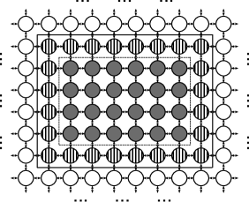
Figure 1: Probability of boundary states and truncation errors. The gray states in the center box of dashed lines form the state space $\Omega^{(\mathcal{B}-\mathbbm{1})}$, with the rest as states truncated from $\Omega^{(\mathcal{B}-\mathbbm{1})}$. The stripe-filled states are the newly added states when the buffer capacity is increased from $\mathcal{B}-\mathbbm{1}$ to $\mathcal{B}$. These new states and those gray states, both enclosed in the box in solid lines, form the state space $\Omega^{(\mathcal{B})}$. The summed true probability mass over the white states outside the solid-lined box is the error $\operatorname{Err}^{(\mathcal{B})}$ of the truncated state space $\Omega^{(\mathcal{B})}$. The summed true probability mass over all states outside of the dashed line box is the error $\operatorname{Err}^{(\mathcal{B}-\mathbbm{1})}$. The summed true probability over stripe-filled states $\pi^{(\mathcal{I})}_{\partial,\,\mathcal{B}}$ is the incremental error $\Delta\operatorname{Err}^{(\mathcal{B})}(t)$ when the buffer capacity of all buffer queues is increased by $1$ from $\mathcal{B}-\mathbbm{1}$. We have: $\pi^{(\mathcal{I})}_{\partial,\,\mathcal{B}}=\Delta\operatorname{Err}^{(\mathcal{B})}(t)=|\operatorname{Err}^{(\mathcal{B})}(t)-\operatorname{Err}^{(\mathcal{B}-\mathbbm{1})}(t)|$.

Incremental truncation errors

The state space $\Omega^{(\mathcal{B})}$ is obtained from enumeration by adding $1$ to the capacity of every buffer queue used to obtain the state space $\Omega^{(\mathcal{B}-\mathbbm{1})}$. Let $\mathbbm{1}=(1,1,\cdots,1)\in\mathbb{Z}^{w}$. The boundary of $\Omega^{(\mathcal{B})}$ can then be written as: $\partial\Omega^{(\mathcal{B})}=\Omega^{(\mathcal{B})}-\Omega^{(\mathcal{B}-\mathbbm{1})}$. It is obvious that the true total boundary probability $\pi^{(\mathcal{I})}_{\partial,\,\mathcal{B}}$ is the increment of the truncation error between $\Omega^{(\mathcal{B}-\mathbbm{1})}$ and $\Omega^{(\mathcal{B})}$:

$$\pi^{(\mathcal{I})}_{\partial,\,\mathcal{B}}=\Delta\operatorname{Err}^{(\mathcal{B})}=\operatorname{Err}^{(\mathcal{B}-\mathbbm{1})}-\operatorname{Err}^{(\mathcal{B})}.$$ (7)

Fig. 1 gives an illustration.

Let ${\mbox{\boldmath$e$}}_{j}=(0,\cdots,0,\,1,\,0,\cdots,0)\in\mathbb{Z}_{\geq 0}^{w}$ be an elementary vector with only the $j$-th element as $1$ and all others $0$. The boundary states of the $j$-th iBD is given by: $\partial\Omega^{(\mathcal{B})}_{(B_{j})}=\Omega^{(\mathcal{B})}-\Omega^{(\mathcal{B}-{\mbox{\boldmath$e$}}_{j})}$. Analogous to Eqn. (7), the boundary probability $\pi^{(\mathcal{I})}_{\partial,\,B_{j}}$ is therefore the increment of the truncation error between $\Omega^{(\mathcal{B}-{\mbox{\boldmath$e$}}_{j})}$ and $\Omega^{(\mathcal{B})}$:

$$\pi^{(\mathcal{I})}_{\partial,\,B_{j}}=\Delta\operatorname{Err}^{(B_{j})}=\operatorname{Err}^{(\mathcal{B}-{\mbox{\boldmath$e$}}_{j})}-\operatorname{Err}^{(\mathcal{B})},$$ (8)

as the only difference between $\Omega^{(\mathcal{B}-{\mbox{\boldmath$e$}}_{j})}$ and $\Omega^{(\mathcal{B})}$ are those states containing exactly $B_{j}$ net synthesized molecules in the $j$-th iBD, namely, the states with the $j$-th buffer queue depleted.

Total true error is no greater than summed errors over all iBDs

Overall, we have $\partial\Omega^{(\mathcal{B})}=\bigcup_{j=1}^{w}\partial\Omega^{(\mathcal{B})}_{(B_{j})}$. As some boundary states may have multiple depleted buffer queues, it is possible $\partial\Omega^{(\mathcal{B})}_{(B_{i})}\cap\partial\Omega^{(\mathcal{B})}_{(B_{j})}\neq\emptyset,\,\cdots,\,\bigcap_{i=1}^{w}\partial\Omega^{(\mathcal{B})}_{(B_{i})}\neq\emptyset.$ Therefore, the actual total boundary probability $\pi^{(\mathcal{I})}_{\partial,\,\mathcal{B}}$ is smaller than or equal to the summation of individual $\pi^{(\mathcal{I})}_{\partial,\,B_{j}}$:

$$\pi^{(\mathcal{I})}_{\partial,\,\mathcal{B}}\leq\sum_{j=1}^{w}\pi^{(\mathcal{I})}(\partial\Omega^{(\mathcal{B})}_{(B_{j})})\equiv\sum_{j=1}^{w}\pi^{(\mathcal{I})}_{\partial,\,B_{j}}.$$ (9)

As the state space $\Omega^{(\mathcal{B})}=\bigcap_{i=1}^{w}\Omega^{(\mathcal{I}_{j})}$ and the buffer capacity of the $j$-th iBD in $\Omega^{(\mathcal{I}_{j})}$ is the same as that in $\Omega^{(\mathcal{B})}$, we have that the total true error of the state space $\Omega^{(\mathcal{B})}$ is bounded by the summation of true errors from individually truncated state spaces $\Omega^{(\mathcal{I}_{j})}$:

$$\operatorname{Err}^{(\mathcal{B})}\leq\sum_{j=1}^{w}\operatorname{Err}^{(\mathcal{I}_{j})}.$$ (10)

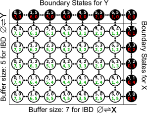
Figure 2: An illustration of the enumerated state space and the boundary states of a simple network with two reactions $\emptyset\rightleftharpoons X$ and $\emptyset\rightleftharpoons Y$. There are two iBDs in this network, with two buffer queues $B_{1}$ and $B_{2}$ of size 5 and 7 assigned to the first and second iBD, respectively. Each circle represents an enumerated state. Filled circles are boundary states, in which at least one of the two buffer queues is depleted. There are four integers inside each circle. The two at the top are copy numbers $x$ and $y$ of molecular species $X$ and $Y$, namely, ${\mbox{\boldmath$x$}}=(x,y)$. The two at the bottom are the remaining numbers $b_{1}$ and $b_{2}$ of tokens in the buffer queues $B_{1}$ and $B_{2}$, namely, ${\mbox{\boldmath$b$}}=(b_{1},b_{2})$.

An example

Fig. 2 shows an example of the enumerated state space using Algorithm 2 for a simple network with reversible reactions $\emptyset\rightleftharpoons X$ and $\emptyset\rightleftharpoons Y$. The network is partitioned into two iBD components, one for $\emptyset\rightleftharpoons X$ and another for $\emptyset\rightleftharpoons Y$. A buffer bank $\mathcal{B}=(B_{1},B_{2})$ with two buffer queues is assigned to the network, with the size vector $(B_{1},\,B_{2})=(7,\,5)$. A synthesis reaction is halted once its buffer queue is depleted, resulting in truncation error. Boundary states, in which at least one of the two buffer queues is depleted, are shown as filled black circles, with states of the buffer queues shown in red numbers. The union of all black filled circles in Fig. 2 form the boundary $\partial\Omega^{(\mathcal{B})}$ of the state space. The boundary states associated with the buffer queue corresponding to the iBD of reaction $\emptyset\rightleftharpoons X$ are:

$$\partial\Omega^{(\mathcal{B})}_{(B_{1})}= \{(x=7,y=5),(x=7,y=4),(x=7,y=3),$$

$$(x=7,y=2),(x=7,y=1),(x=7,y=0)\},$$

in which the buffer queue $B_{1}$ is depleted. The boundary states associated with the iBD of reaction $\emptyset\rightleftharpoons Y$ are:

$$\partial\Omega^{(\mathcal{B})}_{(B_{2})}= \{(x=7,y=5),(x=6,y=5),(x=5,y=5),(x=4,y=5),$$

$$(x=3,y=5),(x=2,y=5),(x=1,y=5),(x=0,y=5)\},$$

in which the buffer queue $B_{2}$ is depleted (Fig. 2). We have $\partial\Omega^{(\mathcal{B})}=\partial\Omega^{(\mathcal{B})}_{(B_{1})}\cup\partial\Omega^{(\mathcal{B})}_{(B_{2})}$. We also observe that $\partial\Omega^{(\mathcal{B})}_{(B_{1})}\cap\partial\Omega^{(\mathcal{B})}_{(B_{2})}=(x=7,y=5)$ is none-empty. Those states that are not on the boundary are shown as unfilled circles.

2.4.4 Bounding Errors Due to A Truncated Buffer Queue

We show how to construct an error bound after truncating an individual buffer queue. We first examine the steady state boundary probability $\pi^{(\mathcal{I}_{j})}_{\partial,B_{j}}$, For ease of discussion, we use $N$ instead of $B_{j}$ to denote the buffer capacity of the $j$-th iBD, and use $\pi_{N}^{(\mathcal{I}_{j})}\equiv\pi^{(\mathcal{I}_{j})}_{\partial,\,B_{j}}$ to denote the boundary probability of $\Omega^{(\mathcal{I}_{j})}$. The true error $\operatorname{Err}^{(\mathcal{I}_{j})}$ associated with buffer bank $\mathcal{I}_{j}=(\infty,\cdots,\infty,B_{j}=N,\infty,\cdots,\infty)$ for the steady state is unknown, as it requires knowledge of $\pi^{(\mathcal{I})}({\mbox{\boldmath$x$}})$ for all ${\mbox{\boldmath$x$}}\in\Omega^{(\mathcal{I})}$. Here, we show that $\operatorname{Err}^{(\mathcal{I}_{j})}$ converges to the true boundary probability $\pi^{(\mathcal{I}_{j})}_{N}$ asymptotically as the size of the buffer queue $N$ increases. Specifically, if the size of the buffer queue is sufficiently large, $\operatorname{Err}^{(\mathcal{I}_{j})}$ is bounded by $\pi^{(\mathcal{I}_{j})}_{N}$ up to a constant factor. As $N$ further increases, $\operatorname{Err}^{(\mathcal{I}_{j})}$ converges to $\pi_{N}^{(\mathcal{I}_{j})}$.

Aggregating states by buffer queue usage

To show how boundary probability $\pi_{N}^{(\mathcal{I}_{j})}$ can be used to construct truncation error bound, we first aggregate states in the original state space $\Omega^{(\mathcal{I}_{j})}$ into $N+1$ non-intersecting subsets according to the net number of tokens in use from buffer $B_{j}$: $\Omega^{(\mathcal{I}_{j})}\equiv\{\mathcal{G}_{0},\mathcal{G}_{1},\cdots,\mathcal{G}_{N}\}$. Here states in each aggregated subset $\mathcal{G}_{s}\subseteq\Omega^{(\mathcal{I}_{j})}$, $s=1,\cdots,N$, all have the same $s$ number of buffer tokens spent from buffer queue $B_{j}$, or equivalently, $(N-s)$ tokens unused in buffer $B_{j}$. Note that each $\mathcal{G}_{s}$ can be of infinite size if the capacity of any other buffer queues are infinite. Conceptually disregard the practical issue of time complexity for now, the states in the state space $\Omega$ can be sorted according to the buffer token from buffer queue $B_{j}$ in use. This can be done using any sorting algorithm, such as the bucket sort algorithm with $N+1$ buckets, with each bucket $\mathcal{G}_{s}$ contain only states with exactly $s$ buffer tokens spent.

With this partition, we can construct a transition rate matrix $\tilde{{\mbox{\boldmath$A$}}}$ from the sorted state space $\Omega^{(\mathcal{I}_{j})}$. The new transition rate matrix $\tilde{{\mbox{\boldmath$A$}}}$ is a permutation of the original dCME matrix $A$ Eqn. (2):

$$\tilde{{\mbox{\boldmath$A$}}}=\left({\begin{array}[]{*{20}c}{{\mbox{\boldmath$A$}}_{0,0}}&{{\mbox{\boldmath$A$}}_{0,1}}&\cdots&{{\mbox{\boldmath$A$}}_{0,N}}\\ {{\mbox{\boldmath$A$}}_{1,0}}&{{\mbox{\boldmath$A$}}_{1,1}}&\cdots&{{\mbox{\boldmath$A$}}_{1,N}}\\ \cdots&\cdots&\cdots&\cdots\\ {{\mbox{\boldmath$A$}}_{N,0}}&{{\mbox{\boldmath$A$}}_{N,1}}&\cdots&{{\mbox{\boldmath$A$}}_{N,N}}\\ \end{array}}\right),$$ (11)

where each block sub-matrix ${\mbox{\boldmath$A$}}_{i,\,j}$ includes all transitions from states in group $\mathcal{G}_{j}$ to states in group $\mathcal{G}_{i}$, and can be defined as: ${\mbox{\boldmath$A$}}_{i,j}=\{{\mbox{\boldmath$a$}}_{m,n}\}_{||\mathcal{G}_{i}||\times||\mathcal{G}_{j}||}$, and each entry ${\mbox{\boldmath$a$}}_{m,n}$ in ${\mbox{\boldmath$A$}}_{i,j}$ is the transition rate from a state ${\mbox{\boldmath$x$}}_{n}\in\mathcal{G}_{j}$ to a state ${\mbox{\boldmath$x$}}_{m}\in\mathcal{G}_{i}$.

Although in principle one can obtain the sorted state space partition $\Omega^{(\mathcal{I}_{j})}\equiv\{\mathcal{G}_{0},\mathcal{G}_{1},\cdots,\mathcal{G}_{N}\}$ and the permuted transition rate matrix $\tilde{{\mbox{\boldmath$A$}}}$, there is no need to do so in practice. The construction of $\Omega^{(\mathcal{I}_{j})}$ and $\tilde{{\mbox{\boldmath$A$}}}$ only serves the purpose for proving lemmas and theorems. Specifically, we only need to know that conceptually the original state space can be sorted and partitioned, and a permuted transition rate matrix $\tilde{{\mbox{\boldmath$A$}}}$ can be constructed from the sorted state space according to the aggregation.

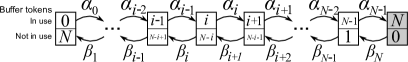
Figure 3: The birth-death system associated with the aggregated rate matrix $B$. Each box represents an aggregated state consisting of all microstates with the same number of buffer tokens in use. The top half of each box lists the number of buffer tokens in use, and the bottom half lists the number of remaining free buffer tokens in the buffer queue. The gray box contains the boundary states. The total number of spent and free tokens sums to the buffer capacity $N$. These aggregated states are connected by aggregated birth and death reactions, with apparent synthesis rates $\alpha_{i}$ and degradation rates $\beta_{i+1}$ (see Fact 2).

Assume the partition and the steady state probability distribution over the state space $\Omega^{(\mathcal{I}_{j})}$ are known, we can construct an aggregated synthesis rate $\alpha^{(N)}_{i}$ for the group $\mathcal{G}_{i}$ and an aggregated degradation rate $\beta^{(N)}_{i+1}$ for the group $\mathcal{G}_{i+1}$ at the steady state as two constants (Fig 3):

$$\alpha^{(N)}_{i}\equiv\left(\mathbbm{1}^{T}{\mbox{\boldmath$A$}}_{i+1,i}\right)\cdot\frac{{\mbox{\boldmath$\pi$}}^{(\mathcal{I}_{j})}(\mathcal{G}_{i})}{\mathbbm{1}^{T}{\mbox{\boldmath$\pi$}}^{(\mathcal{I}_{j})}(\mathcal{G}_{i})}\quad\text{and}\quad\beta^{(N)}_{i+1}\equiv\left(\mathbbm{1}^{T}{\mbox{\boldmath$A$}}_{i,i+1}\right)\cdot\frac{{\mbox{\boldmath$\pi$}}^{(\mathcal{I}_{j})}(\mathcal{G}_{i+1})}{\mathbbm{1}^{T}{\mbox{\boldmath$\pi$}}^{(\mathcal{I}_{j})}(\mathcal{G}_{i+1})},$$ (12)

where vector ${\mbox{\boldmath$\pi$}}^{(\mathcal{I}_{j})}(\mathcal{G}_{i})$ and ${\mbox{\boldmath$\pi$}}^{(\mathcal{I}_{j})}(\mathcal{G}_{i+1})$ are steady state probability vectors over the permuted microstates in the lumped group $\mathcal{G}_{i}$ and $\mathcal{G}_{i+1}$, respectively. Row vectors $\mathbbm{1}^{T}{\mbox{\boldmath$A$}}_{i+1,i}$ and $\mathbbm{1}^{T}{\mbox{\boldmath$A$}}_{i,i+1}$ are summed columns of block sub-matrices ${\mbox{\boldmath$A$}}_{i+1,i}$ and ${\mbox{\boldmath$A$}}_{i,i+1}$, respectively.

Similarly, if the buffer queue $B_{j}$ has infinite capacity, we have

$$\alpha^{(\infty)}_{i}\equiv\left(\mathbbm{1}^{T}{\mbox{\boldmath$A$}}_{i+1,i}\right)\cdot\frac{{\mbox{\boldmath$\pi$}}^{(\mathcal{I})}(\mathcal{G}_{i})}{\mathbbm{1}^{T}{\mbox{\boldmath$\pi$}}^{(\mathcal{I})}(\mathcal{G}_{i})}\quad\text{and}\quad\beta^{(\infty)}_{i+1}\equiv\left(\mathbbm{1}^{T}{\mbox{\boldmath$A$}}_{i,i+1}\right)\cdot\frac{{\mbox{\boldmath$\pi$}}^{(\mathcal{I})}(\mathcal{G}_{i+1})}{\mathbbm{1}^{T}{\mbox{\boldmath$\pi$}}^{(\mathcal{I})}(\mathcal{G}_{i+1})}.$$ (13)

We can then construct an aggregated transition rate matrix $B$ from the permuted matrix $\tilde{{\mbox{\boldmath$A$}}}$ based on Fact 2:

Fact 2

Consider a homogeneous continuous-time Markov process with the infinitesimal generator rate matrix $A$ on the infinite state space $\Omega^{(\mathcal{I}_{j})}$ equipped with buffer queues $\mathcal{I}_{j}=(\infty,\cdots,B_{j},\cdots,\infty)$ with a finite buffer capacity $B_{j}=N$ for the $j$-th iBD, and infinite capacities for all other iBDs. Denote its steady state probability distribution as ${\mbox{\boldmath$\pi$}}^{(\mathcal{I}_{j})}\equiv{\mbox{\boldmath$\pi$}}(\Omega^{(\mathcal{I}_{j})})$. An aggregated continuous-time Markov process with a finite size rate matrix ${\mbox{\boldmath$B$}}_{(N+1)\times(N+1)}$ can be constructed on the partition $\tilde{\Omega}^{(\mathcal{I}_{j})}_{B_{j}}=\{\mathcal{G}_{0},\,\mathcal{G}_{1},\,\cdots,\,\mathcal{G}_{N}\}$ with respect to the buffer queue $B_{j}$. Denote $\tilde{\pi}^{(N)}_{s}\equiv\tilde{\pi}(\mathcal{G}_{s})=\sum_{{\mbox{\boldmath$x$}}\in\mathcal{G}_{s}}\pi^{(\mathcal{I}_{j})}({\mbox{\boldmath$x$}})$. The steady state probability vector $\tilde{{\mbox{\boldmath$\pi$}}}(\tilde{\Omega}^{(\mathcal{I}_{j})}_{B_{j}})=(\tilde{\pi}^{(N)}_{0},\cdots,\tilde{\pi}^{(N)}_{N})=(\tilde{\pi}(\mathcal{G}_{0}),\cdots,\tilde{\pi}(\mathcal{G}_{N}))$ of the aggregated Markov process gives the same steady state probability distribution for the partitioned groups $\{\mathcal{G}_{s}\}$ as that given by the original matrix $A$, for all $s=0,1,\cdots,N$. Furthermore, the $(N+1)\times(N+1)$ transition rate matrix $B$ can be constructed as:

$${\mbox{\boldmath$B$}}^{(N)}=\left({\begin{array}[]{c}\boldsymbol{\alpha}^{(N)},\boldsymbol{\gamma}^{(N)},\boldsymbol{\beta}^{(N)}\end{array}}\right),$$ (14)

with the lower off-diagonal vector

$$\boldsymbol{\alpha}^{(N)}=(\alpha^{(N)}_{i}),\,i=0,\cdots,N-1.$$

the upper off-diagonal vector

$$\boldsymbol{\beta}^{(N)}=(\beta^{(N)}_{i}),\,i=1,\cdots,N.$$

and the diagonal vector

$$\boldsymbol{\gamma}^{(N)}=(\gamma^{(N)}_{i})=(-\alpha^{(N)}_{i}-\beta^{(N)}_{i}),\,i=0,\cdots,N.$$

It is equivalent to transforming the transition rate matrix $\tilde{{\mbox{\boldmath$A$}}}$ in Eqn. (11) to $B$ by substituting each block sub-matrix ${\mbox{\boldmath$A$}}_{i+1,\,i}$ of synthesis reactions with the corresponding aggregated synthesis rate $\alpha^{(N)}_{i}$, and each block ${\mbox{\boldmath$A$}}_{i,\,i+1}$ of degradation reactions with the aggregated degradation rate $\beta^{(N)}_{i+1}$ in Eqn. (12), respectively.

Detailed proof for Fact 2 can be found in Lemma 1 in Ref [42].

Computing steady state boundary probabilities

Following Refs [18, 43] on birth-death processes (Fig. 3), the analytic solution for the steady state $\tilde{\pi}_{i}^{(N)}$ and $\tilde{\pi}_{0}^{(N)}$ can be written as:

$$\tilde{\pi}_{i}^{(N)}=\prod\limits_{k=0}^{i-1}\frac{\alpha^{(N)}_{k}}{\beta^{(N)}_{k+1}}\tilde{\pi}_{0}^{(N)}$$ (15)

and

$$\tilde{\pi}_{0}^{(N)}=\frac{1}{1+{\sum\limits_{j=1}^{N}{\prod\limits_{k=0}^{j-1}{\frac{\alpha^{(N)}_{k}}{\beta^{(N)}_{k+1}}}}}}.$$ (16)

The boundary probability $\tilde{\pi}_{N}^{(N)}$ is then:

$$\tilde{\pi}_{N}^{(N)}\equiv\pi^{(\mathcal{I}_{j})}_{\partial,\,B_{j}}=\frac{\prod\limits_{k=0}^{N-1}\frac{\alpha^{(N)}_{k}}{\beta^{(N)}_{k+1}}}{1+{\sum\limits_{j=1}^{N}{\prod\limits_{k=0}^{j-1}{\frac{\alpha^{(N)}_{k}}{\beta^{(N)}_{k+1}}}}}}.$$ (17)

If we have infinite buffer capacity for the $j$-th iBD, we will have the true probability mass over the same fixed set of states in $\mathcal{G}_{N}$ as

$$\tilde{\pi}_{N}^{(\infty)}\equiv\tilde{\pi}_{N}^{(\mathcal{I})}\equiv\tilde{\pi}_{\partial,\,B_{j}}^{(\mathcal{I})}=\frac{\prod\limits_{k=0}^{N-1}\frac{\alpha^{(\infty)}_{k}}{\beta^{(\infty)}_{k+1}}}{1+{\sum\limits_{j=1}^{\infty}{\prod\limits_{k=0}^{j-1}{\frac{\alpha^{(\infty)}_{k}}{\beta^{(\infty)}_{k+1}}}}}}.$$ (18)

Boundary probability as error bound of state truncation

According to Fact 1, the error $\operatorname{Err}^{(\mathcal{I}_{j})}$ converges to $0$ as the buffer capacity $B_{j}=N$ increases to infinity. For a truncated state space, the series of the true boundary probabilities $\{{\tilde{\pi}^{(\mathcal{I})}_{N}}|N=1,2,\cdots,\}$ (Eqn. (18)) also converges to $0$, as the sequence of its partial sums converges to $1$. That is, the $N$-th member $\ {\tilde{\pi}^{(\mathcal{I})}_{N}}$ of this series converges to $0$ while the residual sum of this series $\operatorname{Err}^{(\mathcal{I}_{j})}\equiv\sum\limits_{i=N+1}^{\infty}{\tilde{\pi}_{i}^{(\infty)}}$ also converges to $0$.

We now examine the convergence behavior of the truncation error $\operatorname{Err}^{(\mathcal{I}_{j})}_{(N)}$ and the true boundary probability $\tilde{\pi}^{(\infty)}_{N}$.

Fact 3

For a truncated state space associated with a buffer bank $\mathcal{I}_{j}$, if the buffer capacity $N$ for queue $B_{j}$ increases to infinity, the truncation error of $B_{j}$ obeys the following inequality:

$$\operatorname{Err}^{(\mathcal{I}_{j})}_{(N)}\leq\frac{\alpha^{(\infty)}_{N}/\beta^{(\infty)}_{N+1}}{1-\alpha^{(\infty)}_{N}/\beta^{(\infty)}_{N+1}}\cdot\tilde{\pi}_{\partial,\,B_{j}}^{(\mathcal{I})}.$$ (19)

Detailed proof for Fact 19 can be found in Theorem 1 in Ref [42].

That is, the true error $\operatorname{Err}^{(\mathcal{I}_{j})}_{(N)}$ is bounded by a simple function of $\alpha^{(\infty)}_{N}$ and $\beta^{(\infty)}_{N+1}$ multiplied by the boundary probability $\tilde{\pi}_{\partial,\,B_{j}}^{(\mathcal{I})}$. We can use this inequality to construct an upper-bound for $\operatorname{Err}^{(\mathcal{I}_{j})}_{(N)}$. We take advantage of the following fact:

Fact 4

For any biological system in which the total amount of mass is finite, e.g., cells with finite mass and growth the aggregated synthesis rate $\alpha^{(\infty)}_{N}$ becomes smaller than the aggregated degradation rate $\beta^{(\infty)}_{N+1}$ when the buffer capacity $N$ is sufficiently large:

$$\lim_{N\rightarrow\infty}\frac{\alpha^{(\infty)}_{N}}{\beta^{(\infty)}_{N+1}}<1.$$

Detailed proof for Fact 4 can be found in Lemma 2 in Ref [42].

Let $C\equiv\frac{\alpha^{(\infty)}_{N}/\beta^{(\infty)}_{N+1}}{1-\alpha^{(\infty)}_{N}/\beta^{(\infty)}_{N+1}}$. If $\alpha^{(\infty)}_{N}/\beta^{(\infty)}_{N+1}<0.5$, we have $C<1$, and the true error $\operatorname{Err}^{(\mathcal{I}_{j})}_{(N)}$ is always less than the true boundary probability $\tilde{\pi}_{\partial,\,B_{j}}^{(\mathcal{I})}$. If $\alpha^{(\infty)}_{N}/\beta^{(\infty)}_{N+1}=0.5$, then $C=1$, and the true error converges asymptotically to the true boundary probability $\tilde{\pi}_{\partial,\,B_{j}}^{(\mathcal{I})}$. If $0.5<\frac{\alpha^{(\infty)}_{N}}{\beta^{(\infty)}_{N+1}}<1.0$, then $C>1$, and the error is larger than $\tilde{\pi}_{\partial,\,B_{j}}^{(\mathcal{I})}$ but is bounded by $\tilde{\pi}_{\partial,\,B_{j}}^{(\mathcal{I})}$ up to the constant factor $C\equiv\frac{\alpha^{(\infty)}_{N}/\beta^{(\infty)}_{N+1}}{1-\alpha^{(\infty)}_{N}/\beta^{(\infty)}_{N+1}}$. Therefore, we can conclude that the true boundary probability $\tilde{\pi}_{\partial,\,B_{j}}^{(\mathcal{I})}$ provides an error bound to the state space truncation.

Note that in real biological reaction networks, the inequality $\alpha^{(\infty)}_{N}/\beta^{(\infty)}_{N+1}<0.5$ usually holds when buffer capacity $N$ is sufficiently large. This is because synthesis reactions usually have constant rates, while rates of degradation reactions depend on the copy number of net molecules in the network. As a result, the ratio between aggregated synthesis and degradation rates decreases monotonically when the total number of molecules in the system increases.

2.4.5 True Boundary Probability and Computed Boundary Probability on Truncated Space

However, it is not possible to calculate the true boundary probability $\tilde{\pi}_{\partial,\,B_{j}}^{(\mathcal{I})}$ on the infinite state space. We have the following fact:

Fact 5

The total probability $\tilde{\pi}_{N}^{(\mathcal{I}_{j})}$ of the boundary states $\partial\Omega^{(\mathcal{I}_{j})}_{B_{j}}$ of the $j$-th iBD with buffer capacity $B_{j}\equiv N$ obtained from the truncated state space $\Omega^{(\mathcal{I}_{j})}$ is greater than or equal to the true probability $\tilde{\pi}_{N}^{(\mathcal{I})}$ over the same boundary states, i.e., $\tilde{\pi}_{N}^{(\mathcal{I})}\leq\tilde{\pi}_{N}^{(\mathcal{I}_{j})}$.

Detailed proof for Fact 5 can be found in Theorem 2 in Ref [42].

We can therefore conclude that the true boundary probability is no greater than the truncated boundary probability given in Eqn. (17) in the general case when $\alpha^{(N)}_{i}\neq 0$ and $\beta^{(N)}_{i+1}\neq 0$. We further consider two additional cases. When reactions associated with the $j$-th iBD has zero synthesis and nonzero degradation constants, namely, $\alpha^{(N)}_{i}=0$ and $\beta^{(N)}_{i+1}\neq 0$, the aggregated system with respect to $j$-th iBD is a death process and there is no synthesis reactions. The associated iBD is closed and a finite buffer works once all states of the closed iBD are enumerated. When reactions associated with the $j$-th iBD has nonzero synthesis but zero degradation constants, we have $\alpha^{(N)}_{i}\neq 0$ but $\beta^{(N)}_{i+1}=0$. The aggregated system with respect to the $j$-th iBD is a birth process without degradation reactions. In this case, the error for the time evolving probability can be estimated using a Poisson distribution with parameter $\alpha^{(N)}_{i}\cdot t$, where $\alpha^{(N)}_{i}$ is the maximum aggregated rate, and $t$ is the elapsed time used for computing the time evolution of the probability landscape [44, 36]. We dispense with details here.

2.4.6 Bounding Errors When Truncating Multiple Buffer Queues

We now consider truncating one additional buffer queue at the $i$-th iBD. We denote the buffer bank as $\mathcal{I}_{i,j}=(\infty,\cdots,B_{i},\cdots,B_{j},\cdots,\infty)$, with $B_{i}$ and $B_{j}$ as the buffer capacities of the $i$-th and $j$-th iBDs, respectively. The rest of the buffer queues all have infinite capacities. We denote the corresponding state space as $\Omega^{\mathcal{I}_{i,j}}$, the transition rate matrix as ${\mbox{\boldmath$A$}}^{\mathcal{I}_{i,j}}$, and the steady state probability distribution as ${\mbox{\boldmath$\pi$}}^{\mathcal{I}_{i,j}}$. We have the fact that the probability of each state in the state space $\Omega^{\mathcal{I}_{i,j}}$ is no less than the corresponding probability on $\Omega^{\mathcal{I}_{j}}$, i.e., $\pi^{\mathcal{I}_{i,j}}({\mbox{\boldmath$x$}})\geq\pi^{\mathcal{I}_{j}}({\mbox{\boldmath$x$}})$ for all ${\mbox{\boldmath$x$}}\in\Omega^{\mathcal{I}_{i,j}}$.

Fact 6

At steady state, ${\mbox{\boldmath$\pi$}}^{\mathcal{I}_{i,j}}\geq{\mbox{\boldmath$\pi$}}^{\mathcal{I}_{j}}$ and ${\mbox{\boldmath$\pi$}}^{\mathcal{I}_{i,j}}\rightarrow{\mbox{\boldmath$\pi$}}^{\mathcal{I}_{j}}$ component-wise over state space $\Omega^{\mathcal{I}_{i,j}}$ when buffer capacity $B_{i}\rightarrow\infty$.

Detailed proof for Fact 6 can be found in Theorem 3 in Ref [42].

That is, the computed boundary probability of the $j$-th iBD after introducing an additional truncation at the $i$-th iBD will be no smaller than when the buffer capacity is sufficiently large. Therefore, the boundary probability from double truncated state space $\Omega^{\mathcal{I}_{i,j}}$ can be conservatively and safely used to bound the truncation error. We can further show by induction that boundary probability computed from state space truncated at multiple iBDs $\Omega^{(\mathcal{B})}$ will not be smaller, and therefore can be used to bound the true boundary probabilities.

Error Bound Inequality

According to Eqn. (10), and Facts 1–6, we have the following inequality to bound the true error of state space truncation using the finite buffer bank $\mathcal{B}=(B_{1},\cdots,B_{w})$:

$$\operatorname{Err}^{(\mathcal{B})}\leq\sum_{j=1}^{w}\operatorname{Err}^{(\mathcal{I}_{j})}\leq\sum_{j=1}^{w}C_{j}\,\tilde{\pi}^{(\mathcal{I})}_{\partial,B_{j}}\leq\sum_{j=1}^{w}C_{j}\,\tilde{\pi}^{(\mathcal{I}_{j})}_{\partial,B_{j}}\leq\sum_{j=1}^{w}C_{j}\,\tilde{\pi}^{(\mathcal{B})}_{\partial,B_{j}},$$ (20)

where $C_{j}\equiv\frac{\alpha^{(\infty)}_{B_{j}-1}/\beta^{(\infty)}_{B_{j}}}{1-\alpha^{(\infty)}_{B_{j}-1}/\beta^{(\infty)}_{B_{j}}}$, $j=1,\cdots,w$, are finite constants for each individual buffer queue.

2.4.7 Upper and Lower Bounds for Steady State Boundary Probability

However, the boundary probability $\tilde{\pi}^{(\mathcal{B})}_{\partial,B_{j}}$ cannot be calculated a priori without solving the dCME. To efficiently estimate if the size of the truncated state space is adequate to compute the steady state probability landscape with errors smaller than a predefined tolerance, we now introduce an easy-to-compute method to obtain the upper- and lower-bounds of the boundary probabilities $\tilde{\pi}^{(N)}_{N}$ a priori without solving the dCME.

Denote the maximum and minimum aggregated synthesis rates from the block sub-matrix ${\mbox{\boldmath$A$}}_{i+1,\,i}$ as $\overline{\alpha}^{(N)}_{i}$ and $\underline{\alpha}^{(N)}_{i}$, respectively. They can be computed as the maximum and minimum element of the row vector obtained from the column sums:

$$\overline{\alpha}^{(N)}_{i}=\max\{\mathbbm{1}^{T}{\mbox{\boldmath$A$}}_{i+1,i}\}\quad\mbox{ and }\quad\underline{\alpha}^{(N)}_{i}=\min\{\mathbbm{1}^{T}{\mbox{\boldmath$A$}}_{i+1,i}\},$$ (21)

respectively. The maximum and minimum aggregated degradation rates can be computed similarly from the block sub-matrix ${\mbox{\boldmath$A$}}_{i,\,i+1}$ as:

$$\overline{\beta}^{(N)}_{i+1}=\max\{\mathbbm{1}^{T}{\mbox{\boldmath$A$}}_{i,i+1}\}\quad\mbox{ and }\quad\underline{\beta}^{(N)}_{i+1}=\min\{\mathbbm{1}^{T}{\mbox{\boldmath$A$}}_{i,i+1}\},$$ (22)

respectively. Note that $\overline{\alpha}^{(N)}_{i}$, $\underline{\alpha}^{(N)}_{i}$, $\overline{\beta}^{(N)}_{i+1}$, and $\underline{\beta}^{(N)}_{i+1}$ can be easily calculated a priori without the need for explicit state enumeration and generation of the partitioned transition rate matrix $\tilde{{\mbox{\boldmath$A$}}}$. The block sub-matrix ${\mbox{\boldmath$A$}}_{i+1,i}$ only contains synthesis reactions, ${\mbox{\boldmath$A$}}_{i,i+1}$ only contains degradation reactions. The maximum total copy numbers of reactants are fixed at each aggregated state group when the maximum buffer capacity is specified, therefore $\overline{\alpha}^{(N)}_{i}$, $\underline{\alpha}^{(N)}_{i}$, $\overline{\beta}^{(N)}_{i+1}$, and $\underline{\beta}^{(N)}_{i+1}$ can be easily calculated by examining the maximum and minimum synthesis and degradation reaction rates. As the original $\alpha^{(N)}_{i}$ and $\beta^{(N)}_{i+1}$ given in Eqn. (12) are weighted sums of vector $\mathbbm{1}^{T}{\mbox{\boldmath$A$}}_{i+1,i}$ and $\mathbbm{1}^{T}{\mbox{\boldmath$A$}}_{i,i+1}$ with regard to the steady state probability distribution $\tilde{{\mbox{\boldmath$\pi$}}}^{(N)}(\mathcal{G}_{i})$, respectively, we have

$$\underline{\alpha}^{(N)}_{i}\leq\alpha^{(N)}_{i}\leq\overline{\alpha}^{(N)}_{i}\quad\mbox{ and }\quad\underline{\beta}^{(N)}_{i+1}\leq\beta^{(N)}_{i+1}\leq\overline{\beta}^{(N)}_{i+1}.$$

We use results from the theory of stochastic ordering for comparing Markov processes to bound $\tilde{\pi}^{(N)}_{N}$. Stochastic ordering “$\leq_{st}$” between two infinitesimal generator matrices ${\mbox{\boldmath$P$}}_{n\times n}$ and ${\mbox{\boldmath$Q$}}_{n\times n}$ of Markov processes is defined as [45, 46]

$${\mbox{\boldmath$P$}}\leq_{st}{\mbox{\boldmath$Q$}}\quad\text{if and only if }\sum_{k=j}^{n}P_{i,k}\leq\sum_{k=j}^{n}Q_{i,k}\text{ for all }i,j.$$

Stochastic ordering between two vectors are similarly defined as:

$${\mbox{\boldmath$p$}}\leq_{st}{\mbox{\boldmath$q$}},\quad\text{if and only if }\sum_{k=j}^{n}p_{k}\leq\sum_{k=j}^{n}q_{k}\text{ for all }j.$$

To derive an upper bound for $\tilde{\pi}^{(N)}_{N}$ in Eqn. (17), we construct a new matrix $\overline{{\mbox{\boldmath$B$}}}$ by replacing $\alpha^{(N)}_{k}$ with the corresponding $\overline{\alpha}^{(N)}_{k}$ and $\beta^{(N)}_{k+1}$ with the corresponding $\underline{\beta}^{(N)}_{k+1}$ in the matrix $B$. Similarly, to derive an lower bound for $\tilde{\pi}^{(N)}_{N}$, we construct the matrix $\underline{{\mbox{\boldmath$B$}}}$ by replacing $\alpha^{(N)}_{k}$ with the corresponding $\underline{\alpha}^{(N)}_{k}$ and replace $\beta^{(N)}_{k+1}$ with $\overline{\beta}^{(N)}_{k+1}$ in $B$. We then have the following stochastic ordering:

$$\underline{{\mbox{\boldmath$B$}}}\leq_{st}{\mbox{\boldmath$B$}}\leq_{st}\overline{{\mbox{\boldmath$B$}}}.$$

All three matrices $\underline{{\mbox{\boldmath$B$}}}$, $B$, and $\overline{{\mbox{\boldmath$B$}}}$ are “$\leq_{st}-\rm{monotone}$” according to the definitions in Truffet [45]. The steady state probability distributions of matrices $\underline{{\mbox{\boldmath$B$}}}$, $B$, and $\overline{{\mbox{\boldmath$B$}}}$ are denoted as ${\mbox{\boldmath$\pi$}}_{\underline{{\mbox{\boldmath$B$}}}}$, ${\mbox{\boldmath$\pi$}}_{{\mbox{\boldmath$B$}}}$, and ${\mbox{\boldmath$\pi$}}_{\overline{{\mbox{\boldmath$B$}}}}$, respectively. They maintain the same stochastic ordering (Theorem 4.1 of Truffet [45]):

$${\mbox{\boldmath$\pi$}}_{\underline{{\mbox{\boldmath$B$}}}}\leq_{st}{\mbox{\boldmath$\pi$}}_{{\mbox{\boldmath$B$}}}\leq_{st}{\mbox{\boldmath$\pi$}}_{\overline{{\mbox{\boldmath$B$}}}}.$$

Therefore, we have the inequality for the $j$-th buffer queue with capacity $N$:

$$\underline{\tilde{\pi}}^{(N)}_{N}\leq\tilde{\pi}^{(N)}_{N}\leq\overline{\tilde{\pi}}^{(N)}_{N}.$$

Here the upper bound $\overline{\tilde{\pi}}^{(N)}_{N}$ is the boundary probability computed from $\tilde{{\mbox{\boldmath$\pi$}}}_{\overline{{\mbox{\boldmath$B$}}}}$, the lower bound $\underline{\tilde{\pi}}^{(N)}_{N}$ is the boundary probability computed from $\tilde{{\mbox{\boldmath$\pi$}}}_{\underline{{\mbox{\boldmath$B$}}}}$, and $\tilde{\pi}^{(N)}_{N}$ is the boundary probability from $\tilde{{\mbox{\boldmath$\pi$}}}_{{\mbox{\boldmath$B$}}}$. From Eqn. (17), the upper bound $\overline{\tilde{\pi}}^{(N)}_{N}$ can be calculated a priori from reaction rates:

$$\overline{\tilde{\pi}}^{(N)}_{N}=\frac{\prod\limits_{k=0}^{N-1}\frac{\overline{\alpha}^{(N)}_{k}}{\underline{\beta}^{(N)}_{k+1}}}{1+{\sum\limits_{j=1}^{N}{\prod\limits_{k=0}^{j-1}{\frac{\overline{\alpha}^{(N)}_{k}}{\underline{\beta}^{(N)}_{k+1}}}}}},$$ (23)

and the lower bound $\underline{\tilde{\pi}}^{(N)}_{N}$ can be calculated as:

$$\underline{\tilde{\pi}}^{(N)}_{N}=\frac{\prod\limits_{k=0}^{N-1}\frac{\underline{\alpha}^{(N)}_{k}}{\overline{\beta}^{(N)}_{k+1}}}{1+{\sum\limits_{j=1}^{N}{\prod\limits_{k=0}^{j-1}{\frac{\underline{\alpha}^{(N)}_{k}}{\overline{\beta}^{(N)}_{k+1}}}}}}.$$ (24)

These are general upper and lower bounds of truncation error valid for any iBD in a reaction network. The upper and lower bounds for the total error of a reaction network with multiple iBDs can be obtained straightforwardly by taking summations of bounds for each individual iBDs:

$$\sum_{i=1}^{w}\underline{\tilde{\pi}}^{(\mathcal{B})}_{B_{i}}\leq\sum_{i=1}^{w}\tilde{\pi}^{(\mathcal{B})}_{B_{i}}\leq\sum_{i=1}^{w}\overline{\tilde{\pi}}^{(\mathcal{B})}_{B_{i}}.$$ (25)

In summary, we have shown from Eqn. (10), Facts 1–6, Eqn. (20), and Eqn. (25) the truncation error of the steady state probability landscape from each individual iBD $\operatorname{Err}^{(B_{j})}$ using finite buffer bank $\mathcal{B}=(B_{1},\cdots,B_{w})$ can be bounded using the following inequality:

$$\begin{split}\operatorname{Err}^{(\mathcal{I}_{j})}\leq C_{j}\,\tilde{\pi}^{(\mathcal{I})}_{\partial,B_{j}}\leq C_{j}\,\tilde{\pi}^{(\mathcal{I}_{j})}_{\partial,B_{j}}\leq C_{j}\,\tilde{\pi}^{(\mathcal{B})}_{\partial,B_{j}}\leq C_{j}\,\overline{\tilde{\pi}}^{(\mathcal{B})}_{B_{j}}\leq\overline{C}_{j}\,\overline{\tilde{\pi}}^{(\mathcal{B})}_{B_{j}}=\frac{\frac{\overline{\alpha}^{(B_{j})}_{B_{j}-1}}{\underline{\beta}^{(B_{j})}_{B_{j}}}}{1-\frac{\overline{\alpha}^{(B_{j})}_{B_{j}-1}}{\underline{\beta}^{(B_{j})}_{B_{j}}}}\cdot\frac{\prod\limits_{k=0}^{B_{j}-1}\frac{\overline{\alpha}^{(B_{j})}_{k}}{\underline{\beta}^{(B_{j})}_{k+1}}}{1+{\sum\limits_{j=1}^{B_{j}}{\prod\limits_{k=0}^{j-1}{\frac{\overline{\alpha}^{(B_{j})}_{k}}{\underline{\beta}^{(B_{j})}_{k+1}}}}}},\end{split}$$ (26)

and the overall truncation error $\operatorname{Err}^{(\mathcal{B})}$ using the finite buffer bank $\mathcal{B}=(B_{1},\cdots,B_{w})$ can therefore be bounded by the following inequality:

$$\begin{split}\operatorname{Err}^{(\mathcal{B})}\leq\sum_{j=1}^{w}\operatorname{Err}^{(\mathcal{I}_{j})}\leq\sum_{j=1}^{w}\overline{C}_{j}\,\overline{\tilde{\pi}}^{(\mathcal{B})}_{B_{j}}=\sum_{j=1}^{w}\frac{\frac{\overline{\alpha}^{(B_{j})}_{B_{j}-1}}{\underline{\beta}^{(B_{j})}_{B_{j}}}}{1-\frac{\overline{\alpha}^{(B_{j})}_{B_{j}-1}}{\underline{\beta}^{(B_{j})}_{B_{j}}}}\cdot\frac{\prod\limits_{k=0}^{B_{j}-1}\frac{\overline{\alpha}^{(B_{j})}_{k}}{\underline{\beta}^{(B_{j})}_{k+1}}}{1+{\sum\limits_{j=1}^{B_{j}}{\prod\limits_{k=0}^{j-1}{\frac{\overline{\alpha}^{(B_{j})}_{k}}{\underline{\beta}^{(B_{j})}_{k+1}}}}}},\end{split}$$ (27)

where $C_{j}\equiv\frac{\alpha^{(\infty)}_{B_{j}-1}/\beta^{(\infty)}_{B_{j}}}{1-\alpha^{(\infty)}_{B_{j}-1}/\beta^{(\infty)}_{B_{j}}}$ and $\overline{C}_{j}\equiv\frac{\overline{\alpha}^{(B_{j})}_{B_{j}-1}/\underline{\beta}^{(B_{j})}_{B_{j}}}{1-\overline{\alpha}^{(B_{j})}_{B_{j}-1}/\underline{\beta}^{(B_{j})}_{B_{j}}}$, $j=1,\cdots,w$, are finite constants for each individual buffer queue, and we have $C_{j}\leq\overline{C}_{j}$ as $\frac{\alpha^{(\infty)}_{B_{j}-1}}{\beta^{(\infty)}_{B_{j}}}\leq\frac{\overline{\alpha}^{(B_{j})}_{B_{j}-1}}{\underline{\beta}^{(B_{j})}_{B_{j}}}$.

2.5 Optimizing Buffer Allocation

2.5.1 Determining Minimal Buffer Sizes Satisfying Pre-defined Error Tolerance

To determine the minimal buffer sizes for the $w$ iBDs so a pre-defined error tolerance $\epsilon$ is satisfied, we first calculate a priori the upper bound from the boundary probability $\overline{\tilde{\pi}}^{(N)}_{N}$ of each iBD using Eqn. (23) for different buffer sizes. The minimal $N$ for each iBD with $\overline{\tilde{\pi}}^{(N)}_{N}<\epsilon/w$ is then chosen as the size of that buffer queue. Other weighted scheme is also possible. We then proceed to enumerate the state space using a buffer bank whose sizes have been thus determined a priori to numerically solve the dCME .

It is possible that this a priori upper bound is overly conservative, and buffer sizes can be further decreased based on numerical results. Specifically, if the boundary probability computed from numerical solution for an iBD with an a priori determined buffer size is much smaller than the pre-defined error tolerance $\epsilon$, it is possible to further decrease the buffer size of that iBD to gain in memory space and improve computing efficiency.

2.5.2 Optimized Memory Allocation Based on Error Bounds

Our method can also be used to optimize the allocation of memory space to improve the accuracy or computing efficiency of the solution to the dCME. When the total size of the state space is fixed, we can allocate buffer capacities for buffer queues differently, so that the total error of the dCME solution is minimized. A simple strategy is to distribute the errors equally to all buffer queues or according to some weight scheme, for example, based on the error bounds of individual iBDs, or the complexity of computing the rates of individual iBDs, or the effects on numerical efficiency. We then determine the buffer size of each iBD. The relative ratio of buffer sizes of different iBDs can be used to allocate memory. When the state space to be enumerated is too large to fit into the computer memory, we can further decrease buffer capacities for all iBDs simultaneously according to the allocation ratio. Such optimization can be done a priori without trial computations.

2.6 Numerical Solutions of dCME

Time-evolving probability landscape

The time evolving probability landscape derived from a dCME of Eqn. (2) can be expressed in the form of a matrix exponential: ${\mbox{\boldmath$p$}}(t)=e^{{\mbox{\boldmath$A$}}t}{\mbox{\boldmath$p$}}(0),$ where ${\mbox{\boldmath$p$}}(0)$ is the initial probability landscape and $A$ is the transition rate matrix over the enumerated state space $\Omega^{(\mathcal{B})}$. Once ${\mbox{\boldmath$p$}}(0)$ is given, ${\mbox{\boldmath$p$}}(t)$ can be calculated using numerical methods such as the Krylov subspace projection method, e.g., as implemented in the Expokit package of Sidjie et al [38]. Other numerical techniques can also be applied [47]. All results of the time-evolving probability landscape in this study are computed using the Expokit package.

Steady state probability landscape

The steady state probability landscape $\pi$ is of great general interests. It is governed by the equation ${\mbox{\boldmath$A$}}{\mbox{\boldmath$\pi$}}=0$, and corresponds to the right eigenvector of the $0$ eigenvalue. With the states enumerated by the mb-dCME method, $\pi$ can be computed using numerical techniques such as iterative solvers [48, 35, 49, 50]. In this study, we use the Gauss-Seidel solver to compute all steady state probability landscape. To our knowledge, the ACME method and its predecessor are the only known methods for computing the steady state probability landscape for an arbitrary biological reaction network.

First passage time distribution

The first passage time from a specific initial state to a given end state is of great importance in studying rare events. The probability that a network transits from the starting state ${\mbox{\boldmath$x$}}_{s}$ to the end state ${\mbox{\boldmath$x$}}_{e}$ within time $t$ is the first passage time probability $p(t,{\mbox{\boldmath$x$}}_{e}|{\mbox{\boldmath$x$}}_{s})$.

The distribution of $p(t,{\mbox{\boldmath$x$}}_{e}|{\mbox{\boldmath$x$}}_{s})$ at all possible time intervals and the corresponding cumulative probability distribution $F(t,{\mbox{\boldmath$x$}}_{e}|{\mbox{\boldmath$x$}}_{s})$, namely, the probability distribution that the system transits from ${\mbox{\boldmath$x$}}_{s}$ to ${\mbox{\boldmath$x$}}_{e}$ within time $t$, can be computed using the ACME method. To obtain $F(t,{\mbox{\boldmath$x$}}_{e}|{\mbox{\boldmath$x$}}_{s})$, we use the absorbing matrix ${\mbox{\boldmath$A$}}_{abs}$ instead of the original rate matrix $A$ by simply replacing the end state ${\mbox{\boldmath$x$}}_{e}$ with an absorbing state [51]. In addition, we assign the initial state ${\mbox{\boldmath$x$}}_{i}$ with a probability of $1$. The time evolving probability landscape of this absorbing system then can be computed as described earlier. The cumulative first passage probabilities $F(t,{\mbox{\boldmath$x$}}_{e}|{\mbox{\boldmath$x$}}_{s})$ at time $t$ is the marginal probability of the end state ${\mbox{\boldmath$x$}}_{e}$ at time $t$ [51]. The probability of a rare event can be easily found from the cumulative distribution of first passage time between the appropriate states.

3 Biological Examples

Below we describe applications using the ACME method in computing the time-evolving and the steady state probability landscapes of several biological reaction networks. We study the genetic toggle switch, the phage lambda lysogenic-lytic epigenetic switch, and the MAPK cascade reaction network. We first show how minimal buffer capacities required for specific error tolerance can be determined a priori. The time-evolving and the steady state probability landscapes of these networks are then computed. We further generate the distributions of first passage times to study the probabilities of rare transition events. Although these three networks are well known, results reported here are significant, as the full stochasticity and the time-evolving probability landscapes have not been computed by solving the underlying dCME for the latter two networks. Furthermore, estimating rare event probabilities such as short first passage time of transition between different states has been a very challenging problem, even for the relatively simple one dimensional Schlögl model [52, 53].

3.1 Genetic Toggle Switch and Its $6$-Dimensional Probability Landscapes

The genetic toggle switch consists of two genes repressing each other through binding of their protein dimeric products on the promoter sites of the other genes. This genetic network has been studied extensively [54, 55, 56, 57]. We follow [57, 35] and study a detailed model of the genetic toggle switch with a more realistic control mechanism of gene regulations. Different from simpler toggle switch models [58, 59, 60, 47], in which gene binding and unbinding reactions are approximated by Hill functions, here detailed negative feedback regulation of gene expressions are modeled explicitly through gene binding and unbinding reactions. Although Hill functions are useful to curve-fit gene regulation models with experimental observations [61], it may be inaccurate to model stochastic networks [61, 62]. It is also difficult to obtain the cooperativity parameters in Hill functions and relate them to the detailed rate constants [61, 62]. Furthermore, Hill function-based model may not capture important multistability characteristics of the reaction network. The genetic toggle switch studied in this example and other previous studies [57, 35] using detailed reaction network with explicit gene binding and unbinding exhibits $4$ distinct stable states (on/off, off/on, on/on, and off/off) for the $GeneX$ and $GeneY$. However, similar genetic toggle switch modeled using Hill function exhibits only two stable states (on/off and off/on) [56, 47].

The molecular species, reactions, and their rate constants for the genetic toggle switch are listed in Table 2. Specifically, two genes $GeneX$ and $GeneY$ express protein products $X$ and $Y$, respectively. Two $X$/$Y$ protein monomers can bind on the promoter site of $GeneY$/$GeneX$ to form protein-DNA complexes $BGeneY$/$BGeneX$, and turn off the expression of $GeneY$/$GeneX$, respectively.

Sizes of buffer queues	mb-dCME	Hypercube method	Reduction factor
Bistable genetic toggle switch
10, 10	400	1,936	4.84
20, 20	1,600	7,056	4.41
30, 30	3,600	15,376	4.27
40, 40	6,400	26,896	4.20
Phage lambda epigenetic switch network
10, 10	2,151	61,952	28.80
20, 20	9,711	225,792	23.25
30, 30	22,671	492,032	21.70
40, 40	41,031	860,672	20.98
MAPK signaling network
$3$, $3$	$2,176$	$4.3\times 10^{9}$	$2.0\times 10^{6}$
$6$, $6$	$209,304$	$3.3\times 10^{13}$	$1.6\times 10^{8}$
$9$, $9$	$6,210,644$	$1.0\times 10^{16}$	$1.6\times 10^{9}$
$14$, $6$	$2,706,935$	$1.1\times 10^{11}$	$4.1\times 10^{4}$

Table 1: Size comparison of enumerated state spaces for the genetic toggle switch, the epigenetic switch network of phage lambda, and the MAPK network. Column 1 lists sizes of buffer queues used in the mb-dCME method, columns 2 and 3 sizes of the space enumerated by the dCME and the traditional hypercube methods, respectively. Column 4 lists the reduction factors using the mb-dCME method over the hypercube method.

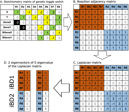
Figure 4: Partitioning the bistable genetic toggle switch network into multiple independent Birth-Death (iBD) components using Algorithm 1. (A) Stoichiometry matrix of the genetic toggle switch constructed from the reaction network in Eqn. (2) in the Appendix. (B) The reaction adjacency matrix constructed from the stoichiometry matrix according to Eqn. (28). (C) The Laplacian matrix of the reaction network constructed using Eqn. (30). There are two 0 eigenvalues for the Laplacian matrix in (C). (D) The 2 eigenvectors corresponding to the two 0 eigenvalues give the partition of the reaction network.

Number of buffer queues and comparison of state space sizes

According to Algorithm 1, there are two iBDs in this network, namely, iBD₁ with reactions $R1$, $R3$, $R5$, and $R7$, and iBD₂ with $R2$, $R4$, $R6$, and $R8$. Each is assigned a separate buffer queue. Detailed steps of iBD partition for the genetic toggle switch network using the Algorithm 1 are illustrated in Fig. 4. In this network, reaction $R1$ generates a new molecule $X$ and does not alter the copy number of all other species. Therefore, row $X$ of column $R1$ is 1 (Fig. 4A), and 0 for all other rows of column $R1$). Reaction $R8$ converts one copy of bound gene $X$ ($BGeneX$) into an unbound gene $X$ ($GeneX$) and generates two copies of $Y$ molecules. Therefore, row $BGeneX$ of column $R8$ in the stoichiometry matrix is -1, row $GeneX$ is 1, and row $Y$ is 2. All other rows of column $R8$ are 0s (Fig. 4A). The remaining column vectors of the stoichiometry matrix for other reactions can be obtained similarly. Each row in the resulting stoichiometry matrix records the stoichiometry of a molecular species participating in all of the reactions. The reaction graph can then be constructed by examining which pairs of reactions share reactant(s) and/or product(s). Molecular species $X$ changes copy numbers in both reaction $R1$ and $R3$, therefore we have the edge $e_{{R1},\,{R3}}=1$ in the reaction graph ${\mbox{\boldmath$G$}}_{R}$. We use an adjacency matrix to encode the graph, and the entry for row $R1$ and column $R3$ is therefore 1 (Fig. 4B). Similarly, $R1$ and $R5$ both involve copy number changes in $X$, hence $e_{{R1},\,{R5}}=1$. As $R1$ and $R7$ also involve copy number changes in $X$, we have $e_{{R1},\,{R7}}=1$. In contrast, as $X$ is the only species that changes copy number in reaction $R1$, and $X$ does not participate either as a reactant or a product with altered copy number in $R2$, $R4$, $R6$, and $R8$, the corresponding entries in the adjacency matrix of ${\mbox{\boldmath$G$}}_{R}$ therefore have 0s as entries. More generally, if the dot product of the stoichiometry vectors of two reactions $R_{i}$ and $R_{j}$ is nonzero, $e_{{Ri},\,{Rj}}=1$, otherwise the entry is zero. Once the full adjacency matrix for the reaction graph is complete (Fig. 4B), the Laplacian matrix (Fig. 4C) can be obtained following Eqn. (30) in the Appendix. The number of the eigenvectors of the Laplacian matrix corresponding to the eigenvalue of 0 gives the number of iBDs in the reaction network, and the non-zero entries of each eigenvector gives the membership of the corresponding iBD (Fig. 4D). In this example of genetic toggle switch, 0 is an eigenvalue of multiplicity of 2 of the Laplacian matrix. The two eigenvectors associated with the eigenvalue of 0 give the two iBDs (Fig. 4D). Specifically, the reactions with nonzero entries in each eigenvector form the corresponding iBD: iBD₁ consists of reactions $R1$, $R3$, $R5$, and $R7$, and iBD₂ consists of $R2$, $R4$, $R6$, and $R8$ (Fig. 4D).

The genetic toggle switch is sufficiently complex to exhibit reduced sizes of the enumerated state spaces using the multi-finite buffer algorithm, when compared with the traditional hypercube method. Table 1 lists the sizes of the state spaces using these two methods. The size of enumerated state space for the hypercube method is the product of the maximum number of possible states of each individual species. For example, when both buffer queues have a buffer capacity of $40$, the state space size is $41^{2}\times 2^{4}=26,896$, in which $40+1=41$ is the total number of all possible different copy numbers of protein $X$ and protein $Y$, and $2^{4}$ is the total different binding and unbinding configurations for each of $GeneX$, $GeneY$, $BGeneX$ and $BGeneY$. The traditional approach generates a state space that is about $4$ times larger than that generated by the mb-dCME method in this case.

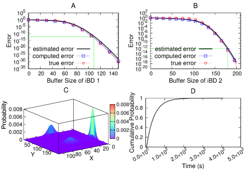
Figure 5: Error estimation and computing the steady state probability landscape and the first passage time of the genetic toggle switch network. (A) and (B): The a priori estimated error (black solid curve), the computed error (blue dashed line and squares), and the true error (red dotted line and circles) of the steady state probability landscape for iBD₁ and iBD₂, respectively. The a priori estimated error is always larger than the computed error. The green dashed lines indicate the estimated minimal buffer size required so the error is within the predefined tolerance of $1\times 10^{-12}$. (C): Steady state probability landscape. (D): The cumulative distribution of the first passage time from the initial state (${\mbox{\boldmath$x$}}_{s}=\{X=49,Y=0,GeneX=1,GeneY=1,BGeneX=0,BGeneY=0\}$) to the end state (${\mbox{\boldmath$x$}}_{e}=\{X=0,Y=99\}$).

Errors and buffer size determinations

The sizes combination of buffer queues ${\mbox{\boldmath$B$}}=(200,400)$ is found to be sufficient to obtain the exact steady state probability landscape (estimated error $<10^{-30}$) according to calculations using Eqn. (23). With the exact steady state probability landscape known, true errors calculated using Eqn. (4) for different sizes of the two buffer queues are shown in Fig. 5A and Fig. 5B (red dotted lines and circles), both of which decrease monotonically with increasing buffer sizes.

The computed error estimates by solving the boundary probability from the underlying dCME (Fig. 5A and B, blue dashed lines and squares) also decrease monotonically with increasing buffer size. The computed error estimates for the 1-st and 2-nd iBD are larger than the true error when the buffer size is larger than $89$ and $163$, respectively, as would be expected from Fact 19.

To estimate a priori the required minimum buffer sizes for both buffer queues for a predefined error tolerance of $\epsilon=1.0\times 10^{-12}$ so that the total error does not exceed $2.0\times 10^{-12}$, we use Eqn. (23) to estimate errors at different buffer sizes (black solid lines in Fig. 5A and B). We follow Eqn. (21) and (22) to compute $\overline{\alpha}_{i}=k_{1}$ and $\underline{\beta}_{(i+1)}=[(i+1)-2]\cdot k_{3}$ for the first iBD, where the subscript $(i+1)$ is the total copy number of species $X$ in the system, and the subtraction of $2$ is necessary because upto $2$ copies of $X$ can be protected from degradation by binding to $GeneY$. This corresponds to the extreme case when $GeneX$ is constantly turned on and $GeneY$ is constantly turned off. The a priori error estimates at different buffer size are shown in Fig. 5A (black solid lines). Similarly, we have $\overline{\alpha}_{i}=k_{2}$ and $\underline{\beta}_{i+1}=[(i+1)-2]\cdot k_{4}$ following Eqn. (21) and (22) for the second iBD. This corresponds to the other extreme case when the $GeneY$ is constantly turned on, and $GeneX$ is constantly turned off (Fig. 5B, black solid lines). As discussed earlier, the a priori estimated error bounds can be easily computed by examining the maximum and minimum reaction rates. There is not need for the transition rate matrix. For both buffer queues, the a priori estimated errors are conservative and are larger than computed errors at all buffer sizes. They are also larger than the true errors when the buffer sizes are sufficiently large. We can therefore determine that the minimal buffer size to satisfy the predefined error tolerance of $\epsilon=2.0\times 10^{-12}$ is $109$ for the first iBD (green dashed lines in Fig. 5A) and $180$ for the second iBD (green dashed lines in Fig. 5B). This combination of buffer sizes ${\mbox{\boldmath$B$}}=(109,180)$ is used for all subsequent calculations. The enumerated state space has a total of $78,480$ states. The $78,480\times 78,480$ transition rate matrix is sparse and contains a total of $468,564$ non-zero elements.

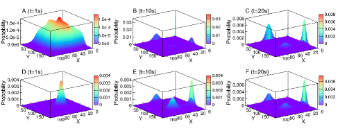
Figure 6: The time evolving probability landscapes of the genetic toggle switch network. (A), (B), and (C): Probability landscapes at $t=1s$, $t=10s$, and $t=20s$, starting from the uniform distribution, respectively. (D), (E), and (F): Probability landscapes at $t=1s$, $t=10s$, and $t=20s$ starting from the initial distribution with $p(X=0,Y=0,GeneX=1,GeneY=1,BGeneX=0,BGeneY=0;t=0)=1$, respectively.

Steady state and time-evolving probability landscapes

The time-evolving probability landscape from two different initial conditions are shown in Fig. 6. We use a time step $\Delta t=0.5s$ and a total simulation time of $t=50s$. The probability landscape in Fig. 6A-C starts from the uniform initial distribution, in which each state takes the same initial probability of $1/78,480$. The probability landscape in Fig. 6D-F starts from an initial probability distribution, in which the state $(X=0,\,Y=0,\,GeneX=1,\,GeneY=1,\,BGeneX=0,\,BGeneY=0)$ has probability $1$ and all other states have probability $0$.

The time-evolving probability landscapes for both initial conditions converges to the same steady state (Fig. 5C) at time $t=40s$, with the computed error for buffer queues 1 and 2 being $1.741\times 10^{-13}$ and $2.881\times 10^{-13}$ for results in Fig. 6A-C, and $1.716\times 10^{-13}$ and $2.898\times 10^{-13}$ for results in Fig. 6D-F, respectively. Note that the Z-scale is different for the time-evolving probability landscapes. The calculation is completed within $2$ minutes using one single core of a 1GHz Quad-Core AMD CPU.

The steady state probability landscape is also computed separately (Fig. 5C for species $X$ and $Y$). It has four peaks that centered at $(X=0,Y=99)$ with a probability of $7.910\times 10^{-3}$; at $(X=49,Y=0)$ with a probability of $2.473\times 10^{-3}$, at $(X=49,Y=99)$ with a probability of $1.269\times 10^{-3}$, and at $(X=0,Y=0)$ with a probability of $5.909\times 10^{-4}$, respectively. The computed error estimates of $1.715\times 10^{-13}$ for the first iBD and $2.899\times 10^{-13}$ for the second iBD are both smaller than the predefined error tolerance of $\epsilon=1.0\times 10^{-12}$. The computing time is within $1$ minute.

First passage time distribution and rare event probabilities

We study the problem of the first passage time when the system travels from the initial starting state ${\mbox{\boldmath$x$}}_{s}=\{X=49,Y=0,GeneX=1,GeneY=1,BGeneX=0,BGeneY=0\}$ to the end state ${\mbox{\boldmath$x$}}_{e}=\{X=0,Y=99\}$. We modified the transition rate matrix by making the end state an absorbing state [51, 32]. The time evolving probability landscape using the absorbing transition rate matrix ${\mbox{\boldmath$A$}}_{abs}$ is then calculated using a time step $\Delta t=0.5$ for a total of $500s$ simulation time.

When the duration is short, the transition from the initial starting state to the end state is of very low probability. When the first passage time is set to $t\leq 3s$, the probability is calculated to be $1.993\times 10^{-5}$, with a computation time of about $10$ seconds. Our method enables accurate and rapid calculations of probabilities of such rare events. As the sampling space of the toggle switch is two-dimension ($X,Y$), the rare event probability estimations in this network is far more challenging than the Schlögl model, which was already beyond the original SSA algorithm [10] and a number of biased stochastic simulation algorithms [29, 52, 30, 63]. To our knowledge, no other methods have succeeded in calculating accurately the rare event probabilities in this model of genetic switch.

The computed full cumulative probability distribution of the first passage time is plotted in Fig. 5D. It increases monotonically with time, and approaching probability $1$. The full calculation is completed within $10$ minutes.

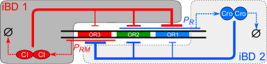
Figure 7: The network model of the lysogeny-lysis decision circuit of phage lambda. CI and Cro proteins can repress the expression of each other by differentially binding to three operator sites (OR1, OR2, and OR3). The network can be partitioned into two iBDs using Algorithm 1, as shown in two shaded areas of different color. There are a total of $11$ molecular species and $50$ reactions in this network (see Table 3 in the Appendix).

3.2 Phage Lambda Epigenetic Switch and Its $11$-Dimensional Probability Landscapes

The epigenetic switch for lysogenic maintenance and lytic induction in phage lambda is a classic problem in systems biology [64]. The efficiency and stability of the decision circuit of the lysogeny-lysis switch have been studied extensively [4, 65, 66, 67, 68]. Here we use a more realistic model of the reaction network adapted from reference [7]. It consists of $11$ molecular species and $50$ reactions. The network diagram is shown in Fig. 7 and detailed reaction schemes and rate constants are based on previous studies [69, 70, 71, 72, 4, 73, 7] and are listed in Table 3 in the Appendix. Molecular species enclosed in parenthesis are required for the specific reactions to occur, but with no changes in stoichiometry. Here $COR(i)$ denotes operator sites OR_i bounded by Cro₂ dimer, $ROR(i)$ for OR_i bounded by CI₂ dimer, $i=1,2,3$.

Number of buffer queues and comparison of state space sizes

There are two iBDs in this network according to Algorithm 1. The first iBD contains all reactions involving $CI$ (dark gray shaded area in Fig. 7), and the second iBD contains all reactions involving $Cro$ (light gray shaded area in Fig. 7). Each iBD is therefore assigned a separate buffer queue.

Table 1 lists the sizes of the state spaces using the mb-dCME method and the traditional hypercube method. As before, the latter is the product of the maximum number of possible states of each individual species. The size of the state space by the traditional approach is about 21–29 times larger than that by the mb-dCME method.

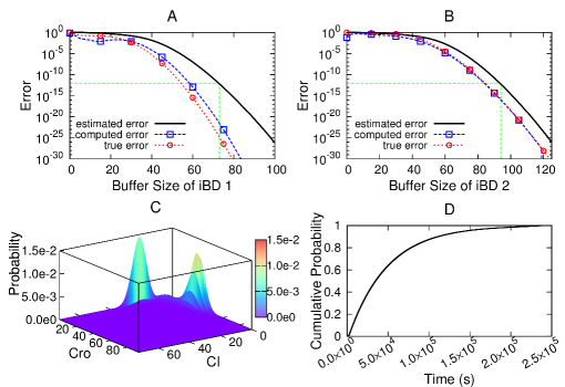
Figure 8: Computing the 11-dimension steady state probability landscape and the first passage time of the network of epigenetic switch of phage lambda. (A) and (B): The a priori estimated error (black solid curve), the computed error (blue dashed line and squares), and the true error (red dotted line and circles) of the steady state probability landscape for iBD₁ and iBD₂, respectively. The computed errors and the true errors are always smaller than the a priori estimated errors. The green dashed lines indicate the estimated minimal buffer sizes required so the error is within the predefined tolerance of $10^{-12}$. (C): The 11-dimensional steady state probability landscape projected onto the $CI$–$Pro$ plane. (D): The cumulative distribution of first passage time from the initial state (${\mbox{\boldmath$x$}}_{s}=\{CI=21,Cro=0,OR1=OR2=OR3=0,ROR1=ROR2=ROR3=0,COR1=COR2=COR3=0\}$) to the end state (${\mbox{\boldmath$x$}}_{e}=\{CI=2,Cro=33\}$).

Errors and buffer size determinations

The size combination of buffer queues of ${\mbox{\boldmath$B$}}=(150,150)$ is sufficient to obtain the exact steady state probability landscape according to calculations using Eqn. (23) (estimated error $<10^{-30}$). The true errors calculated using Eqn. (4) for different sizes of two buffer queues are shown in Fig. 8A and B (red dotted lines and circles), both of which decrease monotonically with increasing buffer size.

The computed error estimates by solving the boundary probability from the underlying dCME (Fig. 8A and B, blue dashed lines and squares) also decrease monotonically with increasing buffer size, when buffer sizes are larger than $23$ and $6$ for the 1-st and 2-nd iBD, respectively. The computed error estimates for the 1-st and 2-nd iBD are larger than the true error when the buffer size is larger than $28$ and $69$, respectively, as would be expected from Fact 19.

To estimate a priori the required minimum buffer sizes for a predefined error tolerance of $\epsilon=1.0\times 10^{-12}$, we use Eqn. (23) to estimate a priori errors at different buffer sizes (black solid lines in Fig. 8A and B). We follow Eqn. (21) and (22) to compute $\overline{\alpha}_{i}=s_{CI}^{1}$ and $\underline{\beta}_{(i+1)}=[(i+1)-6]\cdot d_{CI}$ for the first iBD, where subscript $(i+1)$ is the total copy number of species $CI$ in the system, and the subtraction of $6$ is because there can be maximally $6$ copies of $CI$ molecules protected from degradation by binding on the three operator sites $OR1$, $OR2$, and $OR3$. This corresponds to the extreme case when $CI$ is constantly synthesized at the maximum rate, and degraded at the minimum rate. Similarly, we assign values of $\overline{\alpha}_{i}=s_{Cro}$ and $\underline{\beta}_{i+1}=[(i+1)-6]\cdot d_{Cro}$ in Eqn. (21) and (22) to calculate the estimated error for the 2nd iBD, which corresponds to the other extreme case when the $Cro$ is constantly synthesized at its maximum rate, and degraded at the minimum rate. In both cases, a priori estimated errors are larger than computed errors at all buffer sizes. We can therefore determine conservatively a priori that the minimal buffer size necessary to satisfy the predefined error tolerance of $1.0\times 10^{-12}$ is $73$ for the first iBD (green straight dashed lines in Fig. 8A) and $94$ for the second iBD (green straight dashed lines in Fig. 8B). This combination of buffer sizes ${\mbox{\boldmath$B$}}=(73,94)$ is used for all subsequent calculations. The enumerated state space has a total of $180,756$ states. The $180,756\times 180,756$ transition rate matrix is sparse and contains a total of $1,330,838$ non-zero elements.

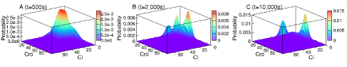
Figure 9: Projection of the 11-dimensional time evolving probability landscape of the epigenetic switch of phage lambda projected to the $CI$–$Cro$ plane starting from the uniform distribution, with the probability landscape (A) at $t=500$s; (B) at $t=2,000$s; and (C) at $t=10,000$s.

Steady state and time-evolving probability landscapes

A projection of the time-evolving 11-dimension probability landscape starting from the uniform initial distribution is shown in Fig. 9, in which each state takes the same initial probability of $1/180,756$. We use a time step $\Delta t=5s$ and a total simulation time of $t=300,000s$. The time-evolving probability landscape converges to the steady state (shown separately on Fig. 8C) at around $t=250,000s$, with the computed error of $1.496\times 10^{-21}$ for buffer queue 1 and $2.722\times 10^{-16}$ for buffer queue 2. The calculation took $18$ hours using one single core of a 1GHz Quad-Core AMD CPU.

The steady state probability landscape is also computed separately. Its projection to the $CI$–$Cro$ plane is plotted in Fig. 8C, which has two peaks centered at $(X=21,Y=0)$, with a probability of $1.447\times 10^{-2}$, and at $(X=2,Y=33)$, with a probability of $1.211\times 10^{-2}$, respectively. The computed error of $1.503\times 10^{-21}$ for the first iBD and $2.711\times 10^{-16}$ for the second iBD are both significantly smaller than the predefined error tolerance of $\epsilon=1.0\times 10^{-12}$. The computation of the steady state probability landscape is completed within $50$ minutes.

First passage time distribution and rare event probabilities

We study the problem of the first passage time when the system travels from the initial state ${\mbox{\boldmath$x$}}_{s}=\{CI=21,Cro=0,OR1=OR2=OR3=0,ROR1=ROR2=ROR3=0,COR1=COR2=COR3=0\}$ in the peak of $CI$ on the $CI-Cro$ plane, to the end state of ${\mbox{\boldmath$x$}}_{e}=\{CI=2,Cro=33\}$, which contains $27$ different microstates at the peak of $Cro$. We modified the transition rate matrix by making these end microstates absorbing [51, 32]. The time evolving probability landscape using the absorbing transition rate matrix ${\mbox{\boldmath$A$}}_{abs}$ is then calculated using a time step $\Delta t=5$ for a total of $250,000s$ simulation time.

When the duration is short, the transition from the initial starting state to the end state is of very low probability. When the first passage time is set to $t\leq 500s$, the probability is calculated to be $7.184\times 10^{-9}$, with a computation time of $9$ minutes. Similar results would require billions of trajectories when using the alternative method of the stochastic simulation algorithm. Similar to the toggle switch example, this rare event problem is two-dimensional ($CI$ and $Cro$), and no current methods we are aware of can accurately calculate such rare event probabilities.

The computed full cumulative probability distribution of the first passage time is plotted in Fig. 8D. It increases monotonically with time, and approaching probability $1$. That is, given enough time, the system will reach the end state ${\mbox{\boldmath$x$}}_{e}=\{X=2,Y=33\}$ with certainty $1$. The full calculation is completed within $25$ hours.

3.3 Bistable MAPK Signaling Cascade and Its $16$-Dimensional Probability Landscapes

The mitogen-activated protein kinase (MAPK) cascades play critical roles in controlling cell responses to external signals and in regulating cell behavior, including proliferation, migration, differentiation, and polarization [74]. There are multiple levels of signal transduction in a MAPK cascade, where activated kinase at each level phosphorylates the kinase at the next level. The MAP kinase is activated by dual phosphorylations at two conserved threonine (T) and tyrosine (Y) residues. Phosphorylated MAPKs can also be dephosphorylated by specific MAP kinase phosphatases (MKPs). Numerous mathematical models have been developed to study the complex behavior of the MAPK cascade in signal transduction [75, 76, 77, 78, 79].

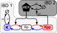
Figure 13: A simplified conceptual model of the MAPK network. The MEK and ERK (K) form a positive feedback loop.

We examine in details both the time-evolving and the steady state probability landscapes of a MAPK cascade model consisting of two levels of kinases, namely, the extracellular signal-regulated kinase (ERK) and its kinase MEK. This network model of $16$ molecular species is an open network, in which the phosphorylation processes for ERK (reactions $R_{5}$ to $R_{21}$ in Table 5) [78], as well as the synthesis and degradation of both ERK and MEK (reactions $R_{1}$ to $R_{4}$ in Table 5) are modeled in details. A feedback loop in the network enhances the synthesis of MEK by activating ERKs (Fig. 13), leading to bistability [79]. The full network is shown in Fig. 10. It includes a total of $16$ molecular species and $35$ individual reactions. Details of the molecular species are listed in Table 4, and reaction schemes and rate constants are specified in Table 5 in Appendix. We set the copy number of MKP3 to $1$ and assume that phosphorylations do not protect the ERK from degradation. To our knowledge, this is the largest network where full stochastic probability landscapes are computed by solving the underlying dCME.

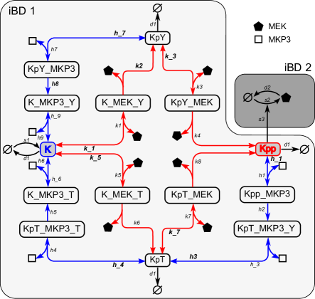
Figure 10: A detailed network model of the MAPK cascade. The ERK(K) phosphorylation is catalyzed by the kinase MEK, whereas MEK synthesis is up-regulated by dual phosphorylated ERK(Kpp). Detailed reactions during the dual phosphorylation process of the ERK(K), the synthesis and degradation of MEK are explicitly modeled. Red and blue arrows represent phosphorylation and dephosphorylation reactions, respectively. Bidirectional arrows represent reversible reactions. The network can be partitioned into two iBDs using Algorithm 1, as shown in two shaded areas of different color. There are a total of $16$ molecular species and $35$ individual reactions in the network (see Tables 4 in Appendix and 5 for more details).

Number of buffer queues and comparison of state space sizes

According to Algorithm 1, there are two iBDs in the network. The first iBD contains all reactions related to the ERK, labeled as $K$, (reactions 3–21 in Table 5 and species in the lightly shaded area in Fig. 10). The second iBD contains reactions of synthesis and degradation of MEK (reactions 1–2 in Table 5 and species in the darkly shaded box in Fig. 10). Each iBD is assigned a separate buffer queue.

To demonstrate the advantage of the mb-dCME state space enumeration method over the traditional hypercube method, Table 1 lists the sizes of the state space with three different choices of the buffer queues. The state spaces generated using the traditional hypercube approach is about $10^{4}$ to $10^{9}$ times larger than that generated by the mb-dCME method. For example, when both buffer queues have a capacity of $9$, the size of the enumerated state space using the traditional hypercube method is $(9+1)^{16}$, in which 16 is the number of molecular species. Compared to the size of $6,210,644$ using the mb-dCME method, the reduction factor is approximately $1.6\times 10^{9}$. Without this dramatic reduction, it would not be feasible to compute the exact probability landscape of this model of MAPK cascade network.

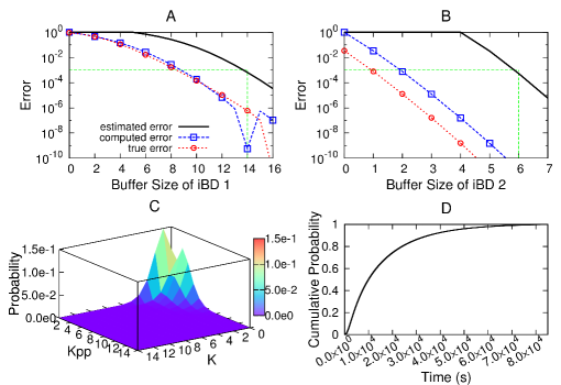
Figure 11: Computing the 16-dimension steady state probability landscape and the first passage time of the MAPK cascade network model. (A) and (B): The a priori estimated error (black solid curve), the computed error (blue dash line and squares), and the true error (red dotted line and circles) of the steady state probability landscape for iBD₁ and iBD₂, respectively. The computed error is significantly smaller than the a priori estimated error. The green straight dashed lines indicate the estimated minimal buffer size required so the error is within the predefined tolerance of $10^{-3}$. (C): The steady state probability landscape projected to the $K$–$K_{pp}$ plane. (D): The cumulative distribution of first passage time from the initial state ($K=3,MKP3=1$) to the end state ($Kpp=2,MKP3=1$).

Errors and buffer size determinations

The size combination of buffer queues ${\mbox{\boldmath$B$}}=(16,7)$ is used to approximate the exact solution to the steady state probability landscape (estimated error $\epsilon<10^{-4}$) according to calculations using Eqn. (23). Although this estimated $\epsilon$ is larger than what is used in other models, it is still quite small, as it is the summation of differences in probabilities of the whole state space. This is due to the complexity of this MAPK model and the limitation of the 3GB CUDA memory of the GPU processor we used. Access to more capable computing facility would allow a different choice of sizes of buffer queues such that a smaller a priori $\epsilon$ can be used. Note that the computed errors for the steady state are considerably smaller ($10^{-8}-10^{-11}$) as described below. With the landscape computed using ${\mbox{\boldmath$B$}}=(16,7)$ regarded as approximately the true steady state probability landscape, the approximated true errors calculated using Eqn. (4) for different sizes of two buffer queues are shown in Fig. 11A and 11B (red dotted lines and circles), both of which decrease monotonically with increasing buffer sizes.

To estimate a priori the required minimum buffer sizes for both buffer queues for a predefined error tolerance of $\epsilon=10^{-3}$, we use Eqn. (23) to estimate errors a priori at different buffer size (black solid lines in Fig. 11A and B). We follow Eqn. (21) and (22) to compute $\overline{\alpha}_{i}=s_{1}$ and $\underline{\beta}_{(i+1)}=[(i+1)-5]\cdot d_{1}$ for the first iBD. Here the subscript $(i+1)$ is the total copy number of ERK. As an ERK molecule can be protected from degradation by forming as many as $5$ copies of ERK-MKP3 and ERK-MEK complexes in our model (one copy for each of the four species involving “$\_MEK\_$”, and one copy for all species involving “$\_MKP3$”, Table 1), the actual minimum degradation rates are conservatively calculated to be $[(i+1)-5]\cdot d_{1}$, where $d_{1}=0.0001$ is the degradation rate of $ERK$ (Table 5). This corresponds to the extreme case when the $ERK$ is constantly synthesized at its maximum rate, and degraded at the minimum rate. Similarly, we have $\overline{\alpha}_{i}=s_{3}$ and $\underline{\beta}_{i+1}=[(i+1)-4]\cdot d_{2}$ for Eqn. (21) and (22) for the 2-nd iBD. As $MEK$ can be protected from degradation by forming as many as of $4$ copies of complexes with $ERK$, the actual minimum degradation rates $\underline{\beta}_{i+1}$ are then conservatively calculated as $[(i+1)-4]\cdot d_{2}$, where $d_{2}=0.15$ is the degradation rate of $MEK$ (Table 5). This corresponds to the other extreme case when the $MEK$ is constantly synthesized at its maximum rate, and degraded at the minimum rate. For both buffer queues, estimated errors are larger than computed errors and true errors at all buffer sizes. We can therefore determine from a priori estimated errors that the minimal buffer size to satisfy the predefined error tolerance $10^{-3}$ is $14$ for the first iBD (green straight dashed lines in Fig. 11A), and $6$ for the second iBD (green straight dashed lines in Fig. 11B). This combination of buffer sizes ${\mbox{\boldmath$B$}}=(14,6)$ is used for all subsequent calculations. The enumerated state space has a total of $2,706,935$ states. The $2,706,935\times 2,706,935$ transition rate matrix is sparse and contains a total of $36,869,845$ non-zero elements.

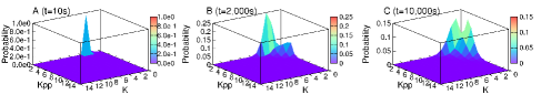
Figure 12: The projected time evolving 16-dimension probability landscape of the MAPK cascade reaction network starting from the initial probability distribution with $p(K=3,MKP3=1,AllOther=0)=1$. (A) The probability landscape projected to the $K$–$K_{pp}$ plane at $t=10s$. (B) Projected probability landscape at $t=2,000s$. (C) Projected probability landscape at $t=10,000s$.

Steady state and time-evolving probability landscapes

The 16-dimension time-evolving probability landscapes starting from the initial probability distribution with $p(K=3,MKP3=1,\rm{others}=0)=1$ are shown in Fig. 12. We use a time step $\Delta t=10s$ and a total simulation time of $t=30,000s$. The time-evolving probability landscape converges to the steady state (Fig. 11C) at about $t=80,000s$. The calculation took $160$ minutes using a GPU workstation with an nVidia GeForce GTX 580 card (3GB CUDA memory) [80].

The steady state probability landscape is also solved separately (Fig. 11C, projected onto the $K$-$Kpp$ plane). It has two peaks centered at $(K=1,Kpp=0)$ with the probability of $0.1495$, and $(K=0,Kpp=2)$ with probability $0.1133$, respectively. The computed errors of $3.447\times 10^{-8}$ for the 1st iBD and $1.335\times 10^{-11}$ for the 2nd iBD are both significantly smaller than the predefined error tolerance of $\epsilon=10^{-3}$. The computation is completed within $50$ minute using the same GPU workstation.

First passage time distribution and rare event probabilities

We study the problem of first passage time when the system travels from an initial start state of ${\mbox{\boldmath$x$}}_{s}=\{K=3,MPK3=1\}$, with all other species $0$ copies, to an end state of ${\mbox{\boldmath$x$}}_{e}=\{Kpp=2,MPK3=1\}$, with all other species $0$ copies. We modified the transition rate matrix by making the end state an absorbing state [51, 32]. The time evolving probability landscape using the absorbing transition rate matrix ${\mbox{\boldmath$A$}}_{abs}$ is then calculated using a time step $\Delta t=1s$ for a total of $85,000s$ simulation time.

When the duration is short, the transition from the initial starting state to the end state is of very low probability. When the first passage time is set to $t\leq 10s$, the probability is calculated to be $6.047\times 10^{-9}$, with a computation time of about $22$ seconds. Similar results would require billions of trajectories when using the alternative method of the stochastic simulation algorithm. As the toggle switch model, this rare event problem is two-dimensional ($K,Kpp$) and no current methods we are aware of can accurately calculate such rare event probabilities.

The computed full cumulative probability distribution of the first passage time is plotted in Fig. 11D. It increases monotonically with time, and approaching probability $1$. That is, given enough time, the system will reach the end state ${\mbox{\boldmath$x$}}_{e}=\{Kpp=2,MPK3=1\}$ with certainty $1$. The full calculation is completed within $41$ hours.

4 Discussions and Conclusions

Direct solution to the discrete chemical master equation (dCME) is of fundamental importance. Because the dCME plays the role in system biology analogous to that of the Schrödinger equation in quantum mechanics [13], developing methods for solving the dCME has important implications, just as developing techniques for solving the Schrödinger equation for systems with many atoms does.

Without the truncation of higher order expansions of the discrete jump operator and without assumptions of lower order noise as in the chemical Langevin and the Fokker-Planck equations, accurate direct computation of the time-evolving as well as the steady state probability landscapes allows the stochastic properties of a biological network to be fully characterized. The overall stochastic behavior of a network, including the presence or absence of multi-stabilities, the often small probabilities of transitions between states, as well as the overall dynamic behavior of the network can all be fully assessed.

A key challenge to obtain direct solution to the dCME is the obstacle of the enormous discrete state space. Conventional hypercube method for state enumeration is easy to implement, but rapidly becomes intractable when the network architecture is nontrivial. In this study, we develop the ACME algorithm using multi-buffers for directly solving the discrete chemical master equation. By decomposing the reaction network into independent components of birth-death processes, multiple buffer queues for these components are employed for more effective state enumeration. With orders of magnitude reduction in the size of the enumerated state space, our algorithm enables accurate solution of the dCME for a large class of problems, whose solutions were previously unobtainable. As the network inside each birth-death component becomes more complex, significant reduction can be achieved. For example, computational studies of the MAPK network shows that a reduction factor of 6–9 orders (e.g., from $1.0\times 10^{16}$ to $6.2\times 10^{6}$ ) can be achieved, allowing a stochastic problem otherwise unsolvable to be computed on a desktop computer.

As truncation of the state space will eventually occur for systems of a given fixed finite buffer capacity with fast synthesis reactions, it is essential to quantify the truncation error and to establish a conservative upper bound of the error, so one can assess whether the computed results are within a predefined error tolerance and are therefore trustworthy. This critically important task is made possible through theoretical analysis of the boundary states and their associated steady state probability, via the construction of an aggregated continuous-time Markov process based on factoring of the state space by the buffer queue usage. With explicit formulae for calculating conservative error bounds for the steady state, one can easily calculate error bounds a priori for a finite state space associated with a given buffer capacity. One can also determine the minimal buffer capacity required if a predefined error tolerance is to be satisfied. This eliminates the need of multiple iterations of costly trial computations to solve the dCME for determining the appropriate buffer capacity necessary to ensure small truncation errors. Furthermore, for a given fixed memory, we can also strategically allocate the memory to different buffer queues so the overall error is minimized, or computing efficiency optimized.

The analysis of the truncation error also enables accurate computation of the steady state probability landscape of a stochastic network. This differs significantly from the finite state projection (FSP) method, which was developed to compute the transient time evolving probability landscape [34, 39]. The FSP method treats all boundary states effectively as one absorbing state, which will eventually trap all probability mass, resulting in a truncation error that can increase to $1$ as time proceeds. The error certificate in the FSP method is used for bounding this leaked probability mass, and requires trial solutions to the dCME, which can be costly. This error certificate therefore may be unsuitable for studying long-time behavior or the steady state of the probability landscape, as time proceeds it approaches to 1.0, and becomes uninformative [34, 39]. In contrast, no absorbing states are introduced in the mb-dCME method, the error bound is based on analysis of the probability mass on the boundary states. To our knowledge, the ACME method is among the first general methods that can directly compute the steady state probabilistic landscape of stochastic networks.

We have also provided computational results of three well-known stochastic networks, namely, the toggle switch, the phage lambda epigenetic circuit, and the MAPK cascade. They are bi- or multi-stable networks. Both the time-evolving and the steady state probability landscapes are computed, all with error less than a predefined threshold. Many biologically critical but rare events, such as the spontaneous induction of latent lysogeny of phage lambda provirus into lysis [7, 65, 81], or the cancerogenesis of a normal cell [82], can in principle be formulated as a problem of estimating the distribution of the first-passage time. The ACME method can be used to directly compute the exact probability of rare events in a stochastic model occurring in an arbitrary time interval. This has been demonstrated in all three examples. Our method can provide solutions to this challenging problem that various forms of specifically designed stochastic simulation algorithms have difficulties to resolve [83, 30, 63, 32].

In this study, we use the Expokit, a Krylov subspace projection method [38], to compute all time-evolving probability landscapes. Exploiting the special structure of the state space, recent development in methods of tensor train decomposition offers another attractive approach to compute the probability landscape by decomposing the dCME transition rate matrix into multiplication of smaller tensors [47]. It would be interesting to explore how this technique can be applied to a state space enumerated by the mb-dCME method. Although the ACME method dramatically reduces the state space and can quantify the truncation error asymptotically, it can still fail when the biological network in question is so large that a reduction factor of $O(n!)$ is insufficient. In addition, the a priori error estimate may not be tight for some complex networks. Further improvements and developments will be the focus of future studies.

Since we have a quantitative estimation of the truncation error, we can be sure that all major probability peaks are contained in the computed solution of probability landscapes when the estimated errors are sufficiently small, as are the cases for the three examples given here. Overall, the goal of this study is to provide a methodology for high precision solutions to the dCME that can be applied to a large class of problems. Important unknown features such as basins, attractors, and transitions for many biological networks can be uncovered, analyzed, and their biological significance assessed. It is now possible to analyze details of the topological, topographical, as well as dynamic properties of the probability landscape for a large number of biologically important stochastic networks that are previously not amenable to computational investigations.

5 ACKNOWLEDGMENTS

This work was supported by NIH grant GM079804, NSF grant MCB1415589, and the Chicago Biomedical Consortium with support from the Searle Funds at The Chicago Community Trust. We thank Dr. Ao Ma for helpful comments, and Alan Perez-Rathke for helpful discussions. YC acknowledges the support of the U.S. Department of Energy through the LANL/LDRD Program for this work. YC thanks Dr. Alan Perelson for helpful comments.

Appendix

Graph of Reaction Network, its Adjacency and Laplacian Matrices

${\mbox{\boldmath$G$}}_{R}$ can be represented by an $m\times m$ adjacency matrix $C$, where:

$${\mbox{\boldmath$C$}}^{m\times m}=||{\mbox{\boldmath$C$}}_{i,\,j}||=\left\{\begin{array}[]{l l}1,&\quad\text{if $e_{ij}$ exists,}\\ 0,&\quad\text{otherwise}\\ \end{array}\right.$$ (28)

The diagonal degree matrix $D$ of the graph ${\mbox{\boldmath$G$}}_{R}$ is:

$${\mbox{\boldmath$D$}}^{m\times m}=||{\mbox{\boldmath$D$}}_{i,\,j}||=\left\{\begin{array}[]{l l}\sum_{k=1}^{m}{{\mbox{\boldmath$C$}}_{i,k}},&\quad\text{if $i=j$},\\ 0,&\quad\text{if $i\neq j$},\\ \end{array}\right.$$ (29)

where each diagonal element ${\mbox{\boldmath$D$}}_{i,i}$ is the vertex degree of the corresponding reaction $R_{i}$. The Laplacian matrix $L$ of the graph ${\mbox{\boldmath$G$}}_{R}$ can be then written as [84]:

$${\mbox{\boldmath$L$}}={\mbox{\boldmath$D$}}-{\mbox{\boldmath$C$}}.$$ (30)

Table 2: Detailed reactions and rate constants of genetic toggle switch.

$R_{1}:GeneX\stackrel{{\scriptstyle k_{1}}}{{\rightarrow}}GeneX+X,\quad k_{1}=50\,s^{-1}$	$R_{3}:X\stackrel{{\scriptstyle k_{3}}}{{\rightarrow}}\emptyset,\quad k_{3}=1\,s^{-1}$
$R_{2}:GeneY\stackrel{{\scriptstyle k_{2}}}{{\rightarrow}}GeneY+Y,\quad k_{2}=100\,s^{-1}$	$R_{4}:Y\stackrel{{\scriptstyle k_{4}}}{{\rightarrow}}\emptyset,\quad k_{4}=1\,s^{-1}$
$R_{5}:2X+GeneY\stackrel{{\scriptstyle k_{5}}}{{\rightarrow}}BGeneY,\quad k_{5}=1\times 10^{-5}\,nM^{-2}\cdot s^{-1}$	$R_{7}:BGeneY\stackrel{{\scriptstyle k_{7}}}{{\rightarrow}}2X+GeneY,\quad k_{7}=0.1\,s^{-1}$
$R_{6}:2Y+GeneX\stackrel{{\scriptstyle k_{6}}}{{\rightarrow}}BGeneX,\quad k_{6}=1\times 10^{-5}\,nM^{-2}\cdot s^{-1}$	$R_{8}:BGeneX\stackrel{{\scriptstyle k_{8}}}{{\rightarrow}}2Y+GeneX,\quad k_{8}=0.1\,s^{-1}$

Table 3: Detailed reactions and rate constants of phage lambda epigenetic switch.

$R_{1}:\emptyset+(OR3+OR2)\stackrel{{\scriptstyle s_{CI}^{0}}}{{\rightarrow}}CI+(OR3+OR2),s_{CI}^{0}=0.0069/s,$	$R_{7}:2CI+OR1\stackrel{{\scriptstyle b_{CI}}}{{\rightarrow}}ROR1,b_{CI}=0.0021/nM^{2}\cdot s,$
$R_{2}:\emptyset+(OR3+COR2)\stackrel{{\scriptstyle s_{CI}^{0}}}{{\rightarrow}}CI+(OR3+COR2),s_{CI}^{0}=0.0069/s,$	$R_{8}:2CI+OR2\stackrel{{\scriptstyle b_{CI}}}{{\rightarrow}}ROR2,b_{CI}=0.0021/nM^{2}\cdot s,$
$R_{3}:\emptyset+(OR3+ROR2)\stackrel{{\scriptstyle s_{CI}^{1}}}{{\rightarrow}}CI+(OR3+ROR2),s_{CI}^{1}=0.066/s,$	$R_{9}:2CI+OR3\stackrel{{\scriptstyle b_{CI}}}{{\rightarrow}}ROR3,b_{CI}=0.0021/nM^{2}\cdot s,$
$R_{4}:\emptyset+(OR1+OR2)\stackrel{{\scriptstyle s_{Cro}}}{{\rightarrow}}Cro+(OR1+OR2),s_{Cro}=0.0929/s,$	$R_{10}:2Cro+OR1\stackrel{{\scriptstyle b_{Cro}}}{{\rightarrow}}COR1,b_{Cro}=0.01289/nM^{2}\cdot s,$
$R_{5}:CI\stackrel{{\scriptstyle d_{CI}}}{{\rightarrow}}\emptyset,d_{CI}=0.0027/s,$	$R_{11}:2Cro+OR2\stackrel{{\scriptstyle b_{Cro}}}{{\rightarrow}}COR2,b_{Cro}=0.01289/nM^{2}\cdot s,$
$R_{6}:Cro\stackrel{{\scriptstyle d_{Cro}}}{{\rightarrow}}\emptyset,d_{Cro}=0.0025/s,$	$R_{12}:2Cro+OR3\stackrel{{\scriptstyle b_{Cro}}}{{\rightarrow}}COR3,b_{Cro}=0.01289/nM^{2}\cdot s,$
$R_{13}:ROR1+(OR2)\stackrel{{\scriptstyle u_{ROR1}}}{{\rightarrow}}2CI+OR1+(OR2),u_{ROR1}=0.03998/s,$
$R_{14}:ROR1+(ROR2+OR3)\stackrel{{\scriptstyle u_{ROR1}^{12}}}{{\rightarrow}}2CI+OR1+(ROR2+OR3),u_{ROR1}^{12}=0.0005/s,$
$R_{15}:ROR1+(ROR2+ROR3)\stackrel{{\scriptstyle u_{ROR1}^{123}}}{{\rightarrow}}2CI+OR1+(ROR2+ROR3),u_{ROR1}^{123}=0.05531/s,$
$R_{16}:ROR1+(ROR2+COR3)\stackrel{{\scriptstyle u_{ROR1}^{12}}}{{\rightarrow}}2CI+OR1+(ROR2+COR3),u_{ROR1}^{12}=0.0005/s,$
$R_{17}:ROR1+(COR2)\stackrel{{\scriptstyle u_{ROR1}}}{{\rightarrow}}2CI+OR1+(COR2),u_{ROR1}=0.03998/s,$
$R_{18}:ROR2+(OR1+OR3)\stackrel{{\scriptstyle u_{ROR2}}}{{\rightarrow}}2CI+OR2+(OR1+OR3),u_{ROR2}=1.026/s,$
$R_{19}:ROR2+(ROR1+OR3)\stackrel{{\scriptstyle u_{ROR2}^{12}}}{{\rightarrow}}2CI+OR2+(ROR1+OR3),u_{ROR2}^{12}=0.01284/s,$
$R_{20}:ROR2+(OR1+ROR3)\stackrel{{\scriptstyle u_{ROR2}^{23}}}{{\rightarrow}}2CI+OR2+(OR1+ROR3),u_{ROR2}^{23}=0.00928/s,$
$R_{21}:ROR2+(ROR1+ROR3)\stackrel{{\scriptstyle u_{ROR2}^{123}}}{{\rightarrow}}2CI+OR2+(ROR1+ROR3),u_{ROR2}^{123}=0.01284/s,$
$R_{22}:ROR2+(COR1+OR3)\stackrel{{\scriptstyle u_{ROR2}}}{{\rightarrow}}2CI+OR2+(COR1+OR3),u_{ROR2}=1.026/s,$
$R_{23}:ROR2+(OR1+COR3)\stackrel{{\scriptstyle u_{ROR2}}}{{\rightarrow}}2CI+OR2+(OR1+COR3),u_{ROR2}=1.026/s,$
$R_{24}:ROR2+(COR1+COR3)\stackrel{{\scriptstyle u_{ROR2}}}{{\rightarrow}}2CI+OR2+(COR1+COR3),u_{ROR2}=1.026/s,$
$R_{25}:ROR2+(ROR1+COR3)\stackrel{{\scriptstyle u_{ROR2}^{12}}}{{\rightarrow}}2CI+OR2+(ROR1+COR3),u_{ROR2}^{12}=0.01284/s,$
$R_{26}:ROR2+(COR1+ROR3)\stackrel{{\scriptstyle u_{ROR2}^{23}}}{{\rightarrow}}2CI+OR2+(COR1+ROR3),u_{ROR2}^{23}=0.00928/s,$
$R_{27}:ROR3+(OR2)\stackrel{{\scriptstyle u_{ROR3}}}{{\rightarrow}}2CI+OR3+(OR2),u_{ROR3}=5.19753/s,$
$R_{28}:ROR3+(ROR2+OR1)\stackrel{{\scriptstyle u_{ROR3}^{23}}}{{\rightarrow}}2CI+OR3+(ROR2+OR1),u_{ROR3}^{23}=0.04702/s,$
$R_{29}:ROR3+(ROR2+ROR1)\stackrel{{\scriptstyle u_{ROR3}^{123}}}{{\rightarrow}}2CI+OR3+(ROR2+ROR1),u_{ROR3}^{123}=5.19753/s,$
$R_{30}:ROR3+(ROR2+COR1)\stackrel{{\scriptstyle u_{ROR3}^{23}}}{{\rightarrow}}2CI+OR3+(ROR2+COR1),u_{ROR3}^{23}=0.04702/s,$
$R_{31}:ROR3+(COR2)\stackrel{{\scriptstyle u_{ROR3}}}{{\rightarrow}}2CI+OR3+(COR2),u_{ROR3}=5.19753/s,$
$R_{32}:COR1+(OR2)\stackrel{{\scriptstyle u_{COR1}}}{{\rightarrow}}2Cro+OR1+(OR2),u_{COR1}=0.08999/s,$
$R_{33}:COR1+(ROR2)\stackrel{{\scriptstyle u_{COR1}}}{{\rightarrow}}2Cro+OR1+(ROR2),u_{COR1}=0.08999/s,$
$R_{34}:COR1+(COR2+OR3)\stackrel{{\scriptstyle u_{COR1}^{12}}}{{\rightarrow}}2Cro+OR1+(COR2+OR3),u_{COR1}^{12}=0.01776/s,$
$R_{35}:COR1+(COR2+ROR3)\stackrel{{\scriptstyle u_{COR1}^{12}}}{{\rightarrow}}2Cro+OR1+(COR2+ROR3),u_{COR1}^{12}=0.01776/s,$
$R_{36}:COR1+(COR2+COR3)\stackrel{{\scriptstyle u_{COR1}^{123}}}{{\rightarrow}}2Cro+OR1+(COR2+COR3),u_{COR1}^{123}=0.05531/s,$
$R_{37}:COR2+(OR1+OR3)\stackrel{{\scriptstyle u_{COR2}}}{{\rightarrow}}2Cro+OR2+(OR1+OR3),u_{COR2}=0.6306/s,$
$R_{38}:COR2+(ROR1+OR3)\stackrel{{\scriptstyle u_{COR2}}}{{\rightarrow}}2Cro+OR2+(ROR1+OR3),u_{COR2}=0.6306/s,$
$R_{39}:COR2+(OR1+ROR3)\stackrel{{\scriptstyle u_{COR2}}}{{\rightarrow}}2Cro+OR2+(OR1+ROR3),u_{COR2}=0.6306/s,$
$R_{40}:COR2+(ROR1+ROR3)\stackrel{{\scriptstyle u_{COR2}}}{{\rightarrow}}2Cro+OR2+(ROR1+ROR3),u_{COR2}=0.6306/s,$
$R_{41}:COR2+(COR1+OR3)\stackrel{{\scriptstyle u_{COR2}^{12}}}{{\rightarrow}}2Cro+OR2+(COR1+OR3),u_{COR2}^{12}=0.12448/s,$
$R_{42}:COR2+(OR1+COR3)\stackrel{{\scriptstyle u_{COR2}^{23}}}{{\rightarrow}}2Cro+OR2+(OR1+COR3),u_{COR2}^{23}=0.23822/s,$
$R_{43}:COR2+(COR1+COR3)\stackrel{{\scriptstyle u_{COR2}^{123}}}{{\rightarrow}}2Cro+OR2+(COR1+COR3),u_{COR2}^{123}=0.14641/s,$
$R_{44}:COR2+(ROR1+COR3)\stackrel{{\scriptstyle u_{COR2}^{23}}}{{\rightarrow}}2Cro+OR2+(ROR1+COR3),u_{COR2}^{23}=0.23822/s,$
$R_{45}:COR2+(COR1+ROR3)\stackrel{{\scriptstyle u_{COR2}^{12}}}{{\rightarrow}}2Cro+OR2+(COR1+ROR3),u_{COR2}^{12}=0.12448/s,$
$R_{46}:COR3+(OR2)\stackrel{{\scriptstyle u_{COR3}}}{{\rightarrow}}2Cro+OR3+(OR2),u_{COR3}=0.00928/s,$
$R_{47}:COR3+(ROR2)\stackrel{{\scriptstyle u_{COR3}}}{{\rightarrow}}2Cro+OR3+(ROR2),u_{COR3}=0.00928/s,$
$R_{48}:COR3+(COR2+OR1)\stackrel{{\scriptstyle u_{COR3}^{23}}}{{\rightarrow}}2Cro+OR3+(COR2+OR1),u_{COR3}^{23}=0.00351/s,$
$R_{49}:COR3+(COR2+ROR1)\stackrel{{\scriptstyle u_{COR3}^{23}}}{{\rightarrow}}2Cro+OR3+(COR2+ROR1),u_{COR3}^{23}=0.00351/s,$
$R_{50}:COR3+(COR2+COR1)\stackrel{{\scriptstyle u_{COR3}^{123}}}{{\rightarrow}}2Cro+OR3+(COR2+COR1),u_{COR3}^{123}=0.01092/s$

Table 4: Molecular species in the network of bistable MAPK signaling cascade.

Molecular species	Descriptions
MEK	ERK kinase
MKP3	ERK phosphatase
K	ERK, extracellular signal-regulated kinase
KpY	Single phosphorylated ERK on Y residue
KpT	Single phosphorylated ERK on T residue
Kpp	Dual phosphorylated ERK on both Y and T residue
K_MEK_Y	K bound by MEK at residue Y
K_MEK_T	K bound by MEK at residue T
KpY_MEK	KpY bound by MEK
KpT_MEK	KpT bound by MEK
Kpp_MKP3	Kpp associated with MKP3
KpY_MKP3	KpY associated with MKP3
KpT_MKP3_Y	KpT associated with MKP3 at residue Y
KpT_MKP3_T	KpT associated with MKP3 at residue T
K_MKP3_T	K associated with MKP3 at residue T
K_MKP3_Y	K associated with MKP3 at residue Y

Table 5: Detailed reactions and rate constants in MAPK signaling network.

$R_{1}:\emptyset\overset{\,s_{2}\,}{\underset{\,d_{2}\,}{\rightleftharpoons}}\text{MEK},s_{2}=0.001/s,d_{2}=0.15/s,$	$R_{2}:\emptyset+\text{(Kpp)}\stackrel{{\scriptstyle s_{3}}}{{\rightarrow}}\text{MEK}+\text{(Kpp)},s_{3}=0.005/s,$
$R_{5}:\text{K}+\text{MEK}\overset{\,k_{1}\,}{\underset{\,k_{-1}\,}{\rightleftharpoons}}\text{K\_MEK\_Y},k_{1}=0.375/nM\cdot s,k_{-1}=1.0/s,$	$R_{3}:\emptyset\overset{\,s_{1}\,}{\underset{\,d_{1}\,}{\rightleftharpoons}}\text{K},s_{1}=0.00024/s,d_{1}=0.0001/s,$
$R_{7}:\text{KpY}+\text{MEK}\overset{\,k_{3}\,}{\underset{\,k_{-3}\,}{\rightleftharpoons}}\text{KpY\_MEK},k_{3}=0.375/nM\cdot s,k_{-3}=1.0/s,$	$R_{4}:\text{KpY}\stackrel{{\scriptstyle d_{1}}}{{\rightarrow}}\emptyset,\text{KpT}\stackrel{{\scriptstyle d_{1}}}{{\rightarrow}}\emptyset,\text{Kpp}\stackrel{{\scriptstyle d_{1}}}{{\rightarrow}}\emptyset,d_{1}=0.0001/s,$
$R_{9}:\text{K}+\text{MEK}\overset{\,k_{5}\,}{\underset{\,k_{-5}\,}{\rightleftharpoons}}\text{K\_MEK\_T},k_{5}=0.375/nM\cdot s,k_{-5}=1.0/s,$	$R_{6}:\text{K\_MEK\_Y}\stackrel{{\scriptstyle k_{2}}}{{\rightarrow}}\text{KpY}+\text{MEK},k_{2}=0.06/s,$
$R_{11}:\text{KpT}+\text{MEK}\overset{\,k_{7}\,}{\underset{\,k_{-7}\,}{\rightleftharpoons}}\text{KpT\_MEK},k_{7}=0.375/nM\cdot s,k_{-7}=1.0/s,$	$R_{8}:\text{KpY\_MEK}\stackrel{{\scriptstyle k_{4}}}{{\rightarrow}}\text{Kpp}+\text{MEK},k_{4}=4.5/s,$
$R_{13}:\text{Kpp}+\text{MKP3}\overset{\,h_{1}\,}{\underset{\,h_{-1}\,}{\rightleftharpoons}}\text{Kpp\_MKP3},h_{1}=0.015/nM\cdot s,h_{-1}=1.0/s,$	$R_{10}:\text{K\_MEK\_T}\stackrel{{\scriptstyle k_{6}}}{{\rightarrow}}\text{KpT}+\text{MEK},k_{6}=0.06/s,$
$R_{15}:\text{KpT\_MKP3\_Y}\overset{\,h_{3}\,}{\underset{\,h_{-3}\,}{\rightleftharpoons}}\text{KpT}+\text{MKP3},h_{3}=0.31/s,h_{-3}=0.01/nM\cdot s,$	$R_{12}:\text{KpT\_MEK}\stackrel{{\scriptstyle k_{8}}}{{\rightarrow}}\text{Kpp}+\text{MEK},k_{8}=4.5/s,$
$R_{16}:\text{KpT}+\text{MKP3}\overset{\,h_{4}\,}{\underset{\,h_{-4}\,}{\rightleftharpoons}}\text{KpT\_MKP3\_T},h_{4}=0.01/nM\cdot s,h_{-4}=1.0/s,$	$R_{14}:\text{Kpp\_MKP3}\stackrel{{\scriptstyle h_{2}}}{{\rightarrow}}\text{KpT\_MKP3\_Y},h_{2}=0.032/s,$
$R_{18}:\text{K\_MKP3\_T}\overset{\,h_{6}\,}{\underset{\,h_{-6}\,}{\rightleftharpoons}}\text{K}+\text{MKP3},h_{6}=0.086/s,h_{-6}=0.0011/nM\cdot s,$	$R_{17}:\text{KpT\_MKP3\_T}\stackrel{{\scriptstyle h_{5}}}{{\rightarrow}}\text{K\_MKP3\_T},h_{5}=0.5/s,$
$R_{19}:\text{KpY}+\text{MKP3}\overset{\,h_{7}\,}{\underset{\,h_{-7}\,}{\rightleftharpoons}}\text{KpY\_MKP3},h_{7}=0.01/nM\cdot s,h_{-7}=1.0/s,$	$R_{20}:\text{KpY\_MKP3}\stackrel{{\scriptstyle h_{8}}}{{\rightarrow}}\text{K\_MKP3\_Y},h_{8}=0.47/s,$
$R_{21}:\text{K\_MKP3\_Y}\overset{\,h_{9}\,}{\underset{\,h_{-9}\,}{\rightleftharpoons}}\text{K}+\text{MKP3},h_{9}=0.14/s,h_{-9}=0.0018/nM\cdot s.$

References

- [1] Ping Ao. Laws in darwinian evolutionary theory. Physics of life Reviews, 2(2):117–156, 2005.
- [2] Jacob Stewart-Ornstein and Hana El-Samad. Stochastic modeling of cellular networks. Computational Methods in Cell Biology, 110:111, 2012.
- [3] Hong Qian. Cooperativity in cellular biochemical processes: noise-enhanced sensitivity, fluctuating enzyme, bistability with nonlinear feedback, and other mechanisms for sigmoidal responses. Annual Review of Biophysics, 41:179–204, 2012.
- [4] Adam Arkin, John Ross, and Harley H. McAdams. Stochastic kinetic analysis of developmental pathway bifurcation in phage -infected Escherichia coli cells. Genetics, 149(4):1633–1648, 1998.
- [5] P.S. Swain, M.B. Elowitz, and E.D. Siggia. Intrinsic and extrinsic contributions to stochasticity in gene expression. Proceedings of the National Academy of Sciences of the United States of America, 99(20):12795, 2002.
- [6] M.B. Elowitz, A.J. Levine, E.D. Siggia, and P.S. Swain. Stochastic gene expression in a single cell. Science, 297(5584):1183, 2002.
- [7] Youfang Cao, Hsiao-Mei Lu, and Jie Liang. Probability landscape of heritable and robust epigenetic state of lysogeny in phage lambda. Proceedings of the National Academy of Sciences of the United States of America, 107(43):18445–18450, 2010.
- [8] H.H. McAdams and A. Arkin. It’s a noisy business! Genetic regulation at the nanomolar scale. Trends in Genetics, 15(2):65–69, 1999.
- [9] Darren J Wilkinson. Stochastic modelling for quantitative description of heterogeneous biological systems. Nature Reviews Genetics, 10(2):122–133, 2009.
- [10] D. T. Gillespie. Exact stochastic simulation of coupled chemical reactions. Journal of Physical Chemistry, 81:2340–2361, 1977.
- [11] Daniel T. Gillespie. A rigorous derivation of the chemical master equation. Physica A, 188:404–425, 1992.
- [12] N.G. Van Kampen. Stochastic processes in physics and chemistry, 3rd Edition. Elsevier Science and Technology books, 2007.
- [13] D.A. Beard and H. Qian. Chemical biophysics: quantitative analysis of cellular systems. Cambridge Univ Pr, 2008.
- [14] Daniel T. Gillespie. A diffusional bimolecular propensity function. The Journal of Chemical Physics, 131(16):–, 2009.
- [15] I.G. Darvey, B.W. Ninham, and P.J. Staff. Stochastic models for second order chemical reaction kinetics. the equilibrium state. The Journal of Chemical Physics, 45:2145–2155, 1966.
- [16] D.A. McQuarrie. Stochastic approach to chemical kinetics. Journal of Applied Probability, 4:413–478, 1967.
- [17] I.J. Laurenzi. An analytical solution of the stochastic master equation for reversible bimolecular reaction kinetics. The Journal of Chemical Physics, 113:3315–3322, 2000.
- [18] Melissa Vellela and Hong Qian. A quasistationary analysis of a stochastic chemical reaction: Keizer’s paradox. Bulletin of Mathematical Biology, 69(5):1727–1746, 2007.
- [19] N. G. Van Kampen. A power series expansion of the master equation. Canadian Journal of Physics, 39(4):551–567, 1961.
- [20] Daniel. T. Gillespie. The chemical langevin equation. The Journal of Chemical Physics, 113:297–306, 2000.
- [21] Daniel T. Gillespie. The chemical Langevin and Fokker−Planck equations for the reversible isomerization reaction†. The Journal of Physical Chemistry A, 106(20):5063–5071, 2002.
- [22] Eric L. Haseltine and James B. Rawlings. Approximate simulation of coupled fast and slow reactions for stochastic chemical kinetics. The Journal of Chemical Physics, 117(15):6959–6969, 2002.
- [23] C. W. Gardiner. Handbook of Stochastic Methods for Physics, Chemistry and the Natural Sciences. Springer, New York, 2004.
- [24] P Ao, D Galas, L Hood, L Yin, and XM Zhu. Towards predictive stochastic dynamical modeling of cancer genesis and progression. Interdisciplinary Sciences: Computational Life Sciences, 2(2):140–144, 2010.
- [25] Jianghong Shi, Tianqi Chen, Ruoshi Yuan, Bo Yuan, and Ping Ao. Relation of a new interpretation of stochastic differential equations to ito process. Journal of Statistical Physics, 148(3):579–590, 2012.
- [26] R. Grima, P. Thomas, and A. V. Straube. How accurate are the nonlinear chemical Fokker-Planck and chemical Langevin equations? The Journal of Chemical Physics, 135(8):084103, Aug 2011.
- [27] P. Thomas, H. Matuschek, and R. Grima. How reliable is the linear noise approximation of gene regulatory networks? BMC Genomics, 14 Suppl 4:S5, 2013.
- [28] R.J. Allen, P.B. Warren, and P.R. Ten Wolde. Sampling rare switching events in biochemical networks. Physical Review Letters, 94(1):18104, 2005.
- [29] H. Kuwahara and I. Mura. An efficient and exact stochastic simulation method to analyze rare events in biochemical systems. The Journal of Chemical Physics, 129:165101, 2008.
- [30] B.J. Daigle, M.K. Roh, D.T. Gillespie, and L.R. Petzold. Automated estimation of rare event probabilities in biochemical systems. The Journal of Chemical Physics, 134:044110, 2011.
- [31] Shuyun Jiao, Yanbo Wang, Bo Yuan, and Ping Ao. Kinetics of muller’s ratchet from adaptive landscape viewpoint. In Systems Biology (ISB), 2011 IEEE International Conference on, pages 27–32. IEEE, 2011.
- [32] Youfang Cao and Jie Liang. Adaptively biased sequential importance sampling for rare events in reaction networks with comparison to exact solutions from finite buffer dCME method. The Journal of Chemical Physics, 139(2):025101, 2013.
- [33] Gaowei Wang, Xiaomei Zhu, Jianren Gu, and Ping Ao. Quantitative implementation of the endogenous molecular–cellular network hypothesis in hepatocellular carcinoma. Interface focus, 4(3):20130064, 2014.
- [34] Brian Munsky and Mustafa Khammash. The finite state projection algorithm for the solution of the chemical master equation. The Journal of Chemical Physics, 124(4):044104, 2006.
- [35] Youfang Cao and Jie Liang. Optimal enumeration of state space of finitely buffered stochastic molecular networks and exact computation of steady state landscape probability. BMC Systems Biology, 2(1):30, 2008.
- [36] Verena Wolf, Rushil Goel, Maria Mateescu, and Thomas Henzinger. Solving the chemical master equation using sliding windows. BMC Systems Biology, 4(1):42, 2010.
- [37] Tobias Jahnke. On reduced models for the chemical master equation. Multiscale Modeling & Simulation, 9(4):1646–1676, 2011.
- [38] Roger B Sidje. Expokit: a software package for computing matrix exponentials. ACM Transactions on Mathematical Software (TOMS), 24(1):130–156, 1998.
- [39] Brian Munsky and Mustafa Khammash. A multiple time interval finite state projection algorithm for the solution to the chemical master equation. Journal of Computational Physics, 226(1):818 – 835, 2007.
- [40] Thomas H Cormen, Charles E Leiserson, Ronald L Rivest, Clifford Stein, et al. Introduction to algorithms, volume 2. MIT press Cambridge, 2001.
- [41] Fan RK Chung. Spectral graph theory, volume 92. American Mathematical Soc., 1997.
- [42] Youfang Cao, Anna Terebus, and Jie Liang. State space truncation with quantified errors for accurate solutions to discrete chemical master equation. Bulletin of Mathematical Biology, page in press, 2016.
- [43] H.M. Taylor and S. Karlin. An Introduction to Stochastic Modeling, 3rd Ed. Academic Press, 1998.
- [44] Bennett L Fox and Peter W Glynn. Computing poisson probabilities. Communications of the ACM, 31(4):440–445, 1988.
- [45] Laurent Truffet. Near complete decomposability: bounding the error by a stochastic comparison method. Advances in Applied Probability, pages 830–855, 1997.
- [46] A Irle. Stochastic ordering for continuous-time processes. Journal of Applied Probability, pages 361–375, 2003.
- [47] Vladimir Kazeev, Mustafa Khammash, Michael Nip, and Christoph Schwab. Direct solution of the chemical master equation using quantized tensor trains. PLoS Computational Biology, 10(3):e1003359, 03 2014.
- [48] R. Lehoucq, D. Sorensen, and C. Yang. Arpack users’ guide: Solution of large scale eigenvalue problems with implicitly restarted Arnoldi methods. SIAM, Philadelphia, 1998.
- [49] W.J. Stewart. Introduction to the numerical solution of Markov chains. Princeton University Press NJ, 1994.
- [50] Youcef Saad and Martin H Schultz. GMRES: A generalized minimal residual algorithm for solving nonsymmetric linear systems. SIAM Journal on Scientific and Statistical Computing, 7(3):856–869, 1986.
- [51] Donald Gross and Douglas R. Miller. The randomization technique as a modeling tool and solution procedure for transient Markov processes. Operations Research, 32(2):343–361, 1984.
- [52] Dan T Gillespie, Min Roh, and Linda R Petzold. Refining the weighted stochastic simulation algorithm. The Journal of Chemical Physics, 130(17):174103, 2009.
- [53] Rory M Donovan, Andrew J Sedgewick, James R Faeder, and Daniel M Zuckerman. Efficient stochastic simulation of chemical kinetics networks using a weighted ensemble of trajectories. The Journal of Chemical Physics, 139(11):115105, 2013.
- [54] Timothy S Gardner, Charles R Cantor, and James J Collins. Construction of a genetic toggle switch in Escherichia coli. Nature, 403(6767):339–342, 2000.
- [55] Thomas B Kepler and Timothy C Elston. Stochasticity in transcriptional regulation: origins, consequences, and mathematical representations. Biophysical Journal, 81(6):3116–3136, 2001.
- [56] Keun-Young Kim and Jin Wang. Potential energy landscape and robustness of a gene regulatory network: toggle switch. PLoS Computational Biology, 3(3):e60, 2007.
- [57] D. Schultz, J. N. Onuchic, and P. G. Wolynes. Understanding stochastic simulations of the smallest genetic networks. The Journal of Chemical Physics, 126(24):245102, 2007.
- [58] Brian Munsky and Mustafa Khammash. The finite state projection approach for the analysis of stochastic noise in gene networks. Automatic Control, IEEE Transactions on, 53(Special Issue):201–214, 2008.
- [59] Peter Deuflhard, Wilhelm Huisinga, T Jahnke, and Michael Wulkow. Adaptive discrete Galerkin methods applied to the chemical master equation. SIAM Journal on Scientific Computing, 30(6):2990–3011, 2008.
- [60] Paul Sjöberg, Per Lötstedt, and Johan Elf. Fokker–Planck approximation of the master equation in molecular biology. Computing and Visualization in Science, 12(1):37–50, 2009.
- [61] Moises Santillán. On the use of the hill functions in mathematical models of gene regulatory networks. Mathematical Modelling of Natural Phenomena, 3(02):85–97, 2008.
- [62] Haseong Kim and Erol Gelenbe. Stochastic gene expression modeling with hill function for switch-like gene responses. IEEE/ACM Transactions on Computational Biology and Bioinformatics, 9(4):973–979, 2012.
- [63] M.K. Roh, B.J. Daigle, D.T. Gillespie, and L.R. Petzold. State-dependent doubly weighted stochastic simulation algorithm for automatic characterization of stochastic biochemical rare events. Journal of Chemical Physics, 135(23):234108, 2011.
- [64] Mark Ptashne. A Genetic Switch: Phage Lambda Revisited. Cold Spring Harbor Laboratory Press; 3 edition, 2004.
- [65] Erik Aurell, Stanley Brown, Johan Johanson, and Kim Sneppen. Stability puzzles in phage . Physical Review E, 65(5):051914, 2002.
- [66] Erik Aurell and Kim Sneppen. Epigenetics as a first exit problem. Physical Review Letters, 88(4):048101, 2002.
- [67] X.-M. Zhu, L. Yin, L. Hood, and P. Ao. Robustness, stability and efficiency of phage lambda genetic switch: dynamical structure analysis. Journal of Bioinformatics and Computational Biology, 2:785–817, 2004.
- [68] X.-M. Zhu, L. Yin, L. Hood, and P. Ao. Calculating biological behaviors of epigenetic states in the phage life cycle. Functional & Integrative Genomics, 4(3):188–195, 2004.
- [69] D. Hawley and W. McClure. In vitro comparison of initiation properties of bacteriophage lambda wild-type PR and x3 mutant promoters. Proceedings of the National Academy of Sciences of the United States of America, 77(11):6381–6385, 1980.
- [70] D. Hawley and W. McClure. Mechanism of activation of transcription initiation from the lambda PRM promoter. Journal of Molecular Biology, 157(3):493–525, 1982.
- [71] Madeline A. Shea and Gary K. Ackers. The control system of bacteriophage lambda a physical-chemical model for gene regulation. Journal of Molecular Biology, 181(2):211–230, 1985.
- [72] M. Li, W. McClure, and M. Susskind. Changing the mechanism of transcriptional activation by phage lambda repressor. Proceedings of the National Academy of Sciences of the United States of America, 94(8):3691–3696, 1997.
- [73] Céline Kuttler and Joachim Niehren. Gene Regulation in the Pi Calculus: Simulating Cooperativity at the Lambda Switch. Transactions on Computational Systems Biology VII, 4230:24–55, 2006.
- [74] Gary L Johnson and Razvan Lapadat. Mitogen-activated protein kinase pathways mediated by erk, jnk, and p38 protein kinases. Science, 298(5600):1911–1912, 2002.
- [75] Chi-Ying Huang and James E Ferrell. Ultrasensitivity in the mitogen-activated protein kinase cascade. Proceedings of the National Academy of Sciences of the United States of America, 93(19):10078–10083, 1996.
- [76] Xiao Wang, Nan Hao, Henrik G Dohlman, and Timothy C Elston. Bistability, stochasticity, and oscillations in the mitogen-activated protein kinase cascade. Biophysical Journal, 90(6):1961–1978, 2006.
- [77] Liang Qiao, Robert B Nachbar, Ioannis G Kevrekidis, and Stanislav Y Shvartsman. Bistability and oscillations in the Huang-Ferrell model of MAPK signaling. PLoS Computational Biology, 3(9):e184, 2007.
- [78] N. I. Markevich, J. B. Hoek, and B. N. Kholodenko. Signaling switches and bistability arising from multisite phosphorylation in protein kinase cascades. The Journal of Cell Biology, 164(3):353–359, 2004.
- [79] Paul Smolen, Douglas A. Baxter, and John H. Byrne. Bistable MAP kinase activity: a plausible mechanism contributing to maintenance of late long-term potentiation. American Journal of Physiology - Cell Physiology, 294(2):C503–C515, 2008.
- [80] Marco Maggioni, Tanya Berger-Wolf, and Jie Liang. Gpu-based steady-state solution of the chemical master equation. In Parallel and Distributed Processing Symposium Workshops & PhD Forum (IPDPSW), 2013 IEEE 27th International, pages 579–588. IEEE, 2013.
- [81] John W. Little, Donald P. Shepley, and David W. Wert. Robustness of a gene regulatory circuit. The EMBO Journal, 18(15):4299–4307, 1999.
- [82] Douglas Hanahan and Robert A Weinberg. The hallmarks of cancer. Cell, 100(1):57–70, 2000.
- [83] Rosalind J Allen, Chantal Valeriani, and Pieter Rein ten Wolde. Forward flux sampling for rare event simulations. Journal of Physics: Condensed Matter, 21(46):463102, 2009.
- [84] Russell Merris. Laplacian matrices of graphs: a survey. Linear Algebra and Its Applications, 197:143–176, 1994.