State space truncation with quantified errors for accurate solutions to discrete Chemical Master Equation

Abstract

The discrete chemical master equation (dCME) provides a general framework for studying stochasticity in mesoscopic reaction networks. Since its direct solution rapidly becomes intractable due to the increasing size of the state space, truncation of the state space is necessary for solving most dCMEs. It is therefore important to assess the consequences of state space truncations so errors can be quantified and minimized. Here we describe a novel method for state space truncation. By partitioning a reaction network into multiple molecular equivalence groups (MEG), we truncate the state space by limiting the total molecular copy numbers in each MEG. We further describe a theoretical framework for analysis of the truncation error in the steady state probability landscape using reflecting boundaries. By aggregating the state space based on the usage of a MEG and constructing an aggregated Markov process, we show that the truncation error of a MEG can be asymptotically bounded by the probability of states on the reflecting boundary of the MEG. Furthermore, truncating states of an arbitrary MEG will not undermine the estimated error of truncating any other MEGs. We then provide an overall error estimate for networks with multiple MEGs. To rapidly determine the appropriate size of an arbitrary MEG, we also introduce an a priori method to estimate the upper bound of its truncation error. This a priori estimate can be rapidly computed from reaction rates of the network, without the need of costly trial solutions of the dCME. As examples, we show results of applying our methods to the four stochastic networks of 1) the birth and death model, 2) the single gene expression model, 3) the genetic toggle switch model, and 4) the phage lambda bistable epigenetic switch model. We demonstrate how truncation errors and steady state probability landscapes can be computed using different sizes of the MEG(s) and how the results validate out theories. Overall, the novel state space truncation and error analysis methods developed here can be used to ensure accurate direct solutions to the dCME for a large number of stochastic networks.

Introduction

Biochemical reaction networks are intrinsically stochastic [1, 2]. Deterministic models based on chemical mass action kinetics cannot capture the stochastic nature of these networks [3, 4, 5]. Instead, the discrete Chemical Master Equation (dCME) that describes the probabilistic reaction jumps between discrete states provides a general framework for fully characterizing mesoscopic stochastic processes in a well mixed system [6, 7, 8, 9, 10]. The steady state and time-evolving probability landscapes over discrete states governed by the dCME provide detailed information of these dynamic stochastic processes. However, the dCME cannot be solved analytically, except for a few very simple cases [11, 12, 13, 14, 15].

The dCME can be approximated using the Fokker-Planck equation (FPE) and the chemical Langevin equation (CLE). These approximations are not applicable when copy numbers are small [16], as relatively large copy numbers of molecules are required for accurate approximation [17, 16, 18, 19, 20]. Recent studies provided assessment of errors in these approximations for several reaction networks [21, 22], as well as numerical demonstration in which the CLE of a 13-node lysogeny-lysis decision network of phage-lambda was found to fail to converge to the correct steady state probability landscape (see appendix of ref [5]). However, consequences of such approximations involving many molecular species and with complex reaction schemes are generally not known.

A widely used approach to study stochasticity is that of stochastic simulation algorithm (SSA) It generates reaction trajectories following the underlying dCME [6], and the stochastic properties of the network can then be inferred through analysis of a large number of simulation trajectories. However, convergence of such simulations is difficult to determine, and the errors in the sampled steady state probability landscape are unknown.

Directly solving the dCME offers another attractive approach. By computing the probability landscape of a stochastic network numerically, its properties, such as those involving rare events, can be studied accurately in details. The finite state projection (FSP) method is among several methods that have been developed to solve dCME directly [23, 24, 25, 26, 5, 27, 28]. The FSP is based on a truncated projection of the state space and uses numerical techniques to compute the time-evolving probability landscapes, which are solutions to the dCME [29, 23, 30]. Although the error due to state space truncation can be calculated for the time-evolving probability landscape [23], the use of an absorbing boundary, to which all truncated states are projected, will lead to the accumulation of errors as time proceeds, and eventually trap all probability mass. The FSP method was designed to study transient behavior of stochastic networks, and is not well suited to study the long-term behavior and the steady state probability landscape of a network.

A bottleneck problem for solving the dCME directly is to have an efficient and adequate account of the discrete state space. As the copy number of each of the $n$ molecular species takes an integer value, conventional hypercube-based methods of state enumeration incorporate all vertices in a $n$-dimensional hypercube non-negative integer lattice, which has an overall size of $O(\prod_{i=1}^{n}{b_{i}})$, where $b_{i}$ is the maximally allowed copy number of molecular species $i$. State enumeration rapidly becomes intractable, both in storage and in computing time. This makes the direct solution of the dCME impossible for many realistic problems. To address this issue, the finite buffer discrete CME (fb-dCME) method was developed for efficient enumeration of the state space [24]. This algorithm is provably optimal in both memory usage and in time required for enumeration. It introduces a buffer queue with a fixed number of molecular tokens to keep track of the remaining number of states that can be enumerated. States with depleted buffer do not absorb probability mass but reflect them to states already enumerated, with the overall probability mass conserved. Further, instead of including every states in a hypercube, it examines only states that can be reached from a given initial state. It can be used to compute the exact steady state and time-evolving probability landscape of a closed network, or an open network when the net gain in newly synthesized molecules does not exceed the predefined finite buffer capacity.

State-space truncation eventually occurs in all methods that directly solve the dCME. For example, it occurs in open systems when no new states can be enumerated, therefore synthesis reaction cannot proceed. However, it is unclear how accurate the probability landscape computed using a truncated state space is. Furthermore, it is unclear how to minimize truncation errors, thus limiting the scope of applications of direct methods such as the fb-dCME method.

In this study, we develop a new method for state space truncation and provide a general theoretical framework for characterizing the error due to state space truncation. We start by partitioning the molecular species in a reaction network into a number of molecular equivalent groups (MEG) according to their chemical compositions. The state space is then truncated by limiting the maximum copy number of each MEG instead of individual molecular species. States with exactly the maximum copy number of a MEG form the reflecting boundary of the state space. We further discuss networks with a single reflecting boundary in the truncated state space. We then show that the total probability of the boundary states can be used as an upper bound of the truncation error in computed steady state probability landscape. This is then generalized to networks with an arbitrary number of reflecting boundaries. We further develop an a priori method derived from stochastic ordering for rapid estimation of the truncation errors of the steady state probability landscape for a given truncated state space. The required maximum copy number of each MEG for a pre-defined error tolerance can also be determined without computing costly trial solutions to the dCME. Overall, the method of state space truncation and the upper bounds of truncation errors established in this study enables accurate quantification of errors in numerical solutions of the dCME, and can help to design strategies so probability landscapes with small and controlled errors can be computed for a large class of biological problems which are previously infeasible.

This paper is organized as follows. We first review basic concepts of the discrete chemical master equation and issues associated with the finite discrete state space. We then describe how to partition a reaction network into molecular equivalent groups and how to truncate the discrete state space. We further discuss truncation errors of the steady state probability landscape and how to construct upper bounds of the truncation errors. This is followed by detailed studies of the single gene expression system and the genetic toggle switch system. We examine the a priori estimated error bound, the computed error, and the true error for different state truncations. We end with discussions and conclusions.

Methods

Theoretical Framework

Reaction Network, State Space and Probability Landscape

In a well-mixed biochemical system with constant volume and temperature, there are $n$ molecular species, denoted as ${\mathcal{X}}=\{X_{1},X_{2},\cdots,X_{n}\}$, and $m$ reactions, denoted as ${\mathcal{R}}=\{R_{1},R_{2},\cdots,R_{m}\}$. Each reaction $R_{k}$ has an intrinsic reaction rate constant $r_{k}$. The microstate of the system at time $t$ is given by the non-negative integer column vector ${\mbox{\boldmath$x$}}(t)\in\mathbb{Z}_{+}^{n}$ of copy numbers of each molecular species: ${\mbox{\boldmath$x$}}(t)=(x_{1}(t),x_{2}(t),\cdots,x_{n}(t))^{T}$, where $x_{i}(t)$ is the copy number of molecular species $X_{i}$ at time $t$. An arbitrary reaction $R_{k}$ with intrinsic rate $r_{k}$ takes the general form of

$$c_{1k}X_{1}+c_{2k}X_{2}+\cdots+c_{nk}X_{n}\overset{r_{k}}{\rightarrow}c^{\prime}_{1k}X_{1}+c^{\prime}_{2k}X_{2}+\cdots+c^{\prime}_{nk}X_{n},$$

which brings the system from a microstate ${\mbox{\boldmath$x$}}_{j}$ to ${\mbox{\boldmath$x$}}_{i}$. The difference between ${\mbox{\boldmath$x$}}_{i}$ and ${\mbox{\boldmath$x$}}_{j}$ is the stoichiometry vector ${\mbox{\boldmath$s$}}_{k}$ of reaction $R_{k}$: ${\mbox{\boldmath$s$}}_{k}={\mbox{\boldmath$x$}}_{i}-{\mbox{\boldmath$x$}}_{j}=(s_{1k},s_{2k},\cdots,s_{nk})^{T}=(c^{\prime}_{1k}-c_{1k},\,c^{\prime}_{2k}-c_{2k},\,\cdots,\,c^{\prime}_{nk}-c_{nk})^{T}\in{\mathbb{Z}}^{n}.$ The rate $A_{k}({\mbox{\boldmath$x$}}_{i},{\mbox{\boldmath$x$}}_{j})$ of reaction $R_{k}$ that brings the microstate from ${\mbox{\boldmath$x$}}_{j}$ to ${\mbox{\boldmath$x$}}_{i}$ is determined by $r_{k}$ and the combination number of relevant reactants in the current microstate ${\mbox{\boldmath$x$}}_{j}$:

$$A_{k}({\mbox{\boldmath$x$}}_{i},{\mbox{\boldmath$x$}}_{j})=A_{k}({\mbox{\boldmath$x$}}_{j})=r_{k}\prod_{l=1}^{n}\binom{x_{l}}{c_{lk}},$$

assuming the convention $\binom{0}{0}=1$.

All possible microstates that a system can visit from a given initial condition form the state space: ${\Omega}=\{{\mbox{\boldmath$x$}}(t)|{\mbox{\boldmath$x$}}(0),\,t\in(0,\,\infty)\}.$ We denote the probability of each microstate at time $t$ as $p({\mbox{\boldmath$x$}}(t))$, and the probability distribution at time $t$ over the full state space as ${{\mbox{\boldmath$p$}}}(t)=\{(p({\mbox{\boldmath$x$}}(t))|{\mbox{\boldmath$x$}}(t)\in\Omega)\}.$ We also call ${{\mbox{\boldmath$p$}}}(t)$ the probability landscape of the network [5].

Discrete Chemical Master Equation

The discrete chemical master equation (dCME) can be written as a set of linear ordinary differential equations describing the change in probability of each discrete state over time:

$$\frac{dp({\mbox{\boldmath$x$}},t)}{dt}=\sum_{{\mbox{\boldmath$x$}}^{\prime},\,{\mbox{\boldmath$x$}}^{\prime}\neq{\mbox{\boldmath$x$}}}[A({\mbox{\boldmath$x$}},{\mbox{\boldmath$x$}}^{\prime})p({\mbox{\boldmath$x$}}^{\prime},t)-A({\mbox{\boldmath$x$}}^{\prime},{\mbox{\boldmath$x$}})p({\mbox{\boldmath$x$}},t)],$$ (1)

Note that $p({\mbox{\boldmath$x$}},t)$ is continuous in time, but is discrete over the state space. In matrix form, the dCME can be written as:

$$\frac{d{\mbox{\boldmath$p$}}(t)}{dt}={\mbox{\boldmath$A$}}{\mbox{\boldmath$p$}}(t),$$ (2)

where ${\mbox{\boldmath$A$}}\in{{\mathbb{R}}}^{|\Omega|\times|\Omega|}$ is the transition rate matrix formed by the collection of all $A({\mbox{\boldmath$x$}}_{i},{\mbox{\boldmath$x$}}_{j})$, which describes the overall reaction rate from state ${\mbox{\boldmath$x$}}_{j}$ to state ${\mbox{\boldmath$x$}}_{i}$:

$$A({\mbox{\boldmath$x$}}_{i},{\mbox{\boldmath$x$}}_{j})=\left\{\begin{array}[]{l l}\sum_{k=1}^{m}A_{k}({\mbox{\boldmath$x$}}_{i},{\mbox{\boldmath$x$}}_{j})&\quad\text{if ${\mbox{\boldmath$x$}}_{i}\neq{\mbox{\boldmath$x$}}_{j}$ and ${\mbox{\boldmath$x$}}_{j}\stackrel{{\scriptstyle R_{k}}}{{\longrightarrow}}{\mbox{\boldmath$x$}}_{i}$},\\ -\sum_{\begin{subarray}{c}{\mbox{\boldmath$x$}}^{\prime}\in\Omega,\\ {\mbox{\boldmath$x$}}^{\prime}\neq{\mbox{\boldmath$x$}}_{j}\end{subarray}}A({\mbox{\boldmath$x$}}^{\prime},{\mbox{\boldmath$x$}}_{j})&\quad\text{if ${\mbox{\boldmath$x$}}_{i}={\mbox{\boldmath$x$}}_{j}$},\\ 0&\quad\text{otherwise}.\\ \end{array}\right.$$ (3)

Molecular Equivalent Groups and Independent Birth-Death Processes

In an open reaction network, synthesis reactions are the only ones that generate new molecules and increase the total mass of the system. Degradation reactions are the only ones that destroy molecules and remove mass from the system. The net copy numbers of various molecular species in an open network gives its total mass. For a given microstate, the mass for each molecular species is defined. The total mass in a network can increase to infinity if synthesis reactions persist. The truncation of the infinite state space of such an open network, which is inevitable due to the limited computing capacity, can lead to errors in computing the probability landscapes of a dCME.

Here we introduce the concept of Molecular Equivalence Groups (MEG), which will be useful for state space truncation. Specifically, molecular species $X_{i}$ and $X_{j}$ belong to the same MEG if $X_{i}$ can be transformed into $X_{j}$ or $X_{j}$ can be transformed into $X_{i}$ through one or more mass-balanced reactions. A stochastic network can have one or more Molecular Equivalent Groups. The total mass of a Molecular Equivalent Group for a specific microstate is defined as the total copy number of the most elementary equivalent molecular species in the Molecular Equivalent Group.

$$A \rightarrow B;\quad 2A \rightarrow C;\quad B+C \rightarrow D;\quad 2X \rightarrow Y;\quad Y \rightarrow Z;\quad$$ (4)

For example, the reaction network shown in Eqn. (4) has two Molecular Equivalent Groups, i.e., $MEG_{1}=\{A,B,C,D\}$ and $MEG_{2}=\{X,Y,Z\}$. The most elementary molecular species in $MEG_{1}$ and $MEG_{2}$ are $A$ and $X$, respectively. For any specific microstate of the network ${\mbox{\boldmath$x$}}=\{a,b,c,d,x,y,z\}$, the total net copy number of the Molecular Equivalent Group $MEG_{1}$ is calculated as $n_{MEG_{1}}({\mbox{\boldmath$x$}})=a+b+2c+3d$, and the total net copy number of $MEG_{2}$ can be calculated as $n_{MEG_{2}}({\mbox{\boldmath$x$}})=x+2y+2z$, where the $a$, $b$, $c$, $d$, $x$, $y$, and $z$ are copy numbers of corresponding molecular species.

We are interested in MEGs containing synthesis and degradation reactions. The set of reactions associated with such an open MEG is called an independent Birth-Death process (iBD). Reactions in an iBD can increase or decrease the total net copy number of molecules in the associated MEG.

State Space Truncation by Molecular Equivalent Group

Here we introduce a novel state truncation method. Instead of truncating the state space by specifying a maximum allowed copy number $B$ for each molecular species, we specify a maximum allowed molecular copy number $B$ for the $j$-th MEG. Assume the $j$-th MEG contains $n_{j}$ distinct molecular species, and conservatively ignore the effects of stoichiometry, the number of all possible states for the $j$-th MEG is then that of the volume of an $n_{j}$-dimensional orthogonal corner simplex, with $B$ the length of all edges with the origin as a vertex. The number of integer lattice nodes in this $n_{j}$-dimensional simplex gives the precise number of states of the $j$-th MEG, which is in turn exactly given by the multiset number $\binom{B+n_{j}}{n_{j}}$. The size of the state space is therefore much smaller than the size of the state space $B^{n_{j}}$ that would be generated by the hypercube method, with a reduction factor of roughly $n_{j}!$ factorial. Note that under the constraint of mass conservation, each molecular species in this MEG can still have a maximum of $B$ copies of molecules.

We further conservatively assume that different MEGs are independent, and each can have maximally $B$ copies of molecules. The size of the overall truncated state space is then $O(\prod_{j}\binom{B+n_{j}}{n_{j}})$. This is much smaller than the $n$-dimensional hypercube, which has an overall size of $O(\prod_{j}B^{n_{j}})=O(B^{n})$, with $n$ the total number of molecular species in the network. Overall, the size of state space generated by MEG truncation can be dramatically smaller than that generated using the hypercube method.

State Space Aggregation According to the Net Copy Number in Molecular Equivalent Group

We first consider the stochastic network with only one Molecular Equivalent Group. We truncate the state space by fixing the maximum amount of total mass in the network. We are interested in estimating the errors due to such a state truncation. To do so, we first factor states in the original state space $\Omega^{(\infty)}$ of infinite size according to the total net copy number of the MEG in each state. The infinite state space $\Omega^{(\infty)}$ can be partitioned into disjoint groups of subsets $\tilde{\Omega}^{(\infty)}\equiv\{\mathcal{G}_{0},\mathcal{G}_{1},\cdots,\mathcal{G}_{N},\cdots\}$, where states in each aggregated subset $\mathcal{G}_{s}$ have exactly the same $s$ total copies of equivalent elementary molecular species of the MEG. The total steady state probability $\tilde{\pi}_{s}^{(\infty)}$ on microstates in each group $\mathcal{G}_{s}$ can then be written as:

$$\tilde{\pi}_{s}^{(\infty)}\equiv\sum_{{\mbox{\boldmath$x$}}\in\mathcal{G}_{s}}\pi^{(\infty)}({\mbox{\boldmath$x$}})=\sum_{{\mbox{\boldmath$x$}}\in\mathcal{G}_{s}}p^{(\infty)}({\mbox{\boldmath$x$}},\,t=\infty).$$ (5)

Based on the state space partition $\tilde{\Omega}^{(\infty)}$, we can re-construct a transition rate matrix $\tilde{{\mbox{\boldmath$A$}}}$, which is a permutation of the original dCME matrix $A$ in Eqn. (2):

$$\tilde{{\mbox{\boldmath$A$}}}=\left({\begin{array}[]{*{20}c}{{\mbox{\boldmath$A$}}_{i,j}}\end{array}}\right),\quad 0\leq i,j\leq\infty$$ (6)

where each block sub-matrix ${\mbox{\boldmath$A$}}_{i,\,j}$ includes all transitions from states in group $\mathcal{G}_{j}$ to states in $\mathcal{G}_{i}$.

In continuous time Markov model of mesoscopic systems, reactions occur instantaneously, and the synthesis and degradation reactions always generate or destroy one molecule at a time. This also applies to oligomers, which are assumed to form only upon association of monomers already synthesized, and dissociate into monomers first before full degradation. The re-constructed matrix $\tilde{{\mbox{\boldmath$A$}}}$ is thus a tri-diagonal block matrix, i.e., ${\mbox{\boldmath$A$}}_{i,\,j}$ is all 0s if $|i-j|>1$. Moreover, synthesis reactions always appear as lower blocks ${\mbox{\boldmath$A$}}_{i+1,\,i}$, and degradation reactions always as upper blocks ${\mbox{\boldmath$A$}}_{i,\,i+1}$. Diagonal blocks ${\mbox{\boldmath$A$}}_{i,\,i}$ contains all coupling reactions that do not alter the net number of synthesized molecules. Note that every ${\mbox{\boldmath$A$}}_{i+1,\,i}$ block and ${\mbox{\boldmath$A$}}_{i,\,i+1}$ block only includes synthesis and degradation reactions associated with the current MEG. For analysis of networks with multiple MEGs, we assume at this time there is no limit on the total mass of other MEGs, therefore the state space is not truncated on these MEGs. These other MEGs do not alter the total net copy number of molecular species in the current MEG.

Note that the assumption of the stoichiometric coefficient of 1 for synthesis and degradation is only for constructing the proofs of the theorems. In computation, there is no condition on the stoichiometry of any reaction, and our method is general and can be applied to any reaction network.

We can obtain the steady state probability $\tilde{\pi}_{s}^{(\infty)}$ on aggregated states without solving the dCME. It is tempting to lump all microstates in each group $\mathcal{G}_{j}$ into one state and replace the original $|\Omega^{(\infty)}|\times|\Omega^{(\infty)}|$ rate matrix $\tilde{{\mbox{\boldmath$A$}}}$ with an aggregated matrix to study the dynamic changes of the probability landscape on this aggregated state space. However, stringent requirements must be satisfied for such lumped states to follow a Markov process [31, 32, 33, 34, 35, 36]. Specifically, a transition rate matrix $A$ for a continuous Markov process is lumpable with respect to a partition $\tilde{\Omega}^{(\infty)}$ if and only if for all pairs of $\mathcal{G}_{s},\,\mathcal{G}_{t}\in\tilde{\Omega}^{(\infty)}$, the condition

$$\sum_{{\mbox{\boldmath$x$}}_{k}\in\mathcal{G}_{t}}A_{ik}=\sum_{{\mbox{\boldmath$x$}}_{k}\in\mathcal{G}_{t}}A_{jk}$$ (7)

holds for all ${\mbox{\boldmath$x$}}_{i},\,{\mbox{\boldmath$x$}}_{j}\in\mathcal{G}_{s}$ [31]. In other words, every state in $\mathcal{G}_{s}$ must have the same total transition rate to group $\mathcal{G}_{t}$, and this must be true for all $\mathcal{G}_{s}$ and $\mathcal{G}_{t}$ [31].

While $\tilde{{\mbox{\boldmath$A$}}}$ does not satisfy this strong condition in general, we can instead construct a lumped transition matrix $B$, which is associated with the aggregated state space derived from the partition $\tilde{\Omega}^{(\infty)}$, such that the aggregated steady state probability distribution on the partition $\tilde{\Omega}^{(\infty)}$ computed from the lumped matrix $B$ is equal to that derived from the steady state distribution computed from the original matrix $A$. That is, steady state probabilities on partitioned groups in $\tilde{\Omega}^{(\infty)}$ are identical using either $B$ or the original $A$.

Assume the steady state probability distribution $\tilde{{\mbox{\boldmath$\pi$}}}({\mbox{\boldmath$x$}})$ over the partitioned state space $\tilde{\Omega}^{(\infty)}$ is known, the aggregated synthesis rate $\alpha^{(\infty)}_{i}$ for the group $\mathcal{G}_{i}$ and the aggregated degradation rate $\beta^{(\infty)}_{i+1}$ for the group $\mathcal{G}_{i+1}$ at the steady state are two constants (Fig 2) defined as

$$\alpha^{(\infty)}_{i}=\left(\mathbbm{1}^{T}{\mbox{\boldmath$A$}}_{i+1,i}\right)\cdot\frac{\tilde{{\mbox{\boldmath$\pi$}}}(\mathcal{G}_{i})}{\mathbbm{1}^{T}\tilde{{\mbox{\boldmath$\pi$}}}(\mathcal{G}_{i})}\quad\text{and}\quad\beta^{(\infty)}_{i+1}=\left(\mathbbm{1}^{T}{\mbox{\boldmath$A$}}_{i,i+1}\right)\cdot\frac{\tilde{{\mbox{\boldmath$\pi$}}}(\mathcal{G}_{i+1})}{\mathbbm{1}^{T}\tilde{{\mbox{\boldmath$\pi$}}}(\mathcal{G}_{i+1})},$$ (8)

where $\tilde{{\mbox{\boldmath$\pi$}}}(\mathcal{G}_{i})$ and $\tilde{{\mbox{\boldmath$\pi$}}}(\mathcal{G}_{i+1})$ are the steady state probability vector over microstates in the lumped states $\mathcal{G}_{i}$ and $\mathcal{G}_{i+1}$, respectively. The term $\mathbbm{1}^{T}{\mbox{\boldmath$A$}}_{i+1,i}$ is the row vector of column-summed rates from ${\mbox{\boldmath$A$}}_{i+1,i}$ for microstates in $\mathcal{G}_{i}$, and $\frac{\tilde{{\mbox{\boldmath$\pi$}}}(\mathcal{G}_{i})}{\mathbbm{1}^{T}\tilde{{\mbox{\boldmath$\pi$}}}(\mathcal{G}_{i})}$ is the steady state probability vector $\tilde{{\mbox{\boldmath$\pi$}}}(\mathcal{G}_{i})$ over microstates in $\mathcal{G}_{i}$ normalized by the total steady state probability on $\mathcal{G}_{i}$. Similarly, $\mathbbm{1}^{T}{\mbox{\boldmath$A$}}_{i,i+1}$ is the row vector of column-summed rates from ${\mbox{\boldmath$A$}}_{i,i+1}$ for microstates in $\mathcal{G}_{i+1}$, and $\frac{\tilde{{\mbox{\boldmath$\pi$}}}(\mathcal{G}_{i+1})}{\mathbbm{1}^{T}\tilde{{\mbox{\boldmath$\pi$}}}(\mathcal{G}_{i+1})}$ is the steady state probability vector $\tilde{{\mbox{\boldmath$\pi$}}}(\mathcal{G}_{i+1})$ over microstates in $\mathcal{G}_{i+1}$ normalized by the total steady state probability on $\mathcal{G}_{i+1}$. We can construct an aggregated transition rate matrix $B$ from $\tilde{{\mbox{\boldmath$A$}}}$ based on the following Lemma:

Lemma 1

(Rate Matrix Aggregation.) If an Molecular Equivalence Group has no limit on the total copy number, it generates an infinite state space $\Omega^{(\infty)}$ and the rate matrix $A$ is of infinite dimension. For any homogeneous continuous-time Markov process with such a rate matrix $A$, an aggregated continuous-time Markov process with an infinite rate matrix ${\mbox{\boldmath$B$}}^{(\infty)}$ can be constructed on the partition $\tilde{\Omega}^{(\infty)}=\{\mathcal{G}_{0},\mathcal{G}_{1},\cdots,\mathcal{G}_{N},\cdots\}$ with respect to the total net copy number of molecules in the network, such that it gives the same steady state probability distribution for each partitioned group $\{\mathcal{G}_{s}\}$ as that given by the original matrix $A$, i.e., $\pi(\mathcal{G}_{s})=\sum_{{\mbox{\boldmath$x$}}\in\mathcal{G}_{s}}{\mbox{\boldmath$\pi$}}({\mbox{\boldmath$x$}})$ for all $s=0,1,\cdots$, where ${\mbox{\boldmath$\pi$}}(\Omega^{(\infty)})$ is the steady state probability distribution associated with $A$. Specifically, the infinite transition rate matrix ${\mbox{\boldmath$B$}}^{(\infty)}$ can be constructed as a tridiagonal matrix:

$${\mbox{\boldmath$B$}}=\left({\begin{array}[]{c}\boldsymbol{\alpha}^{(\infty)},\boldsymbol{\gamma}^{(\infty)},\boldsymbol{\beta}^{(\infty)}\end{array}}\right),$$ (9)

with the lower off-diagonal vector $\boldsymbol{\alpha}^{(\infty)}=(\alpha^{(\infty)}_{i})$, the upper off-diagonal vector $\boldsymbol{\beta}^{(\infty)}=(\beta^{(\infty)}_{i+1})$, and the diagonal vector $\boldsymbol{\gamma}^{(\infty)}=(\gamma^{(\infty)}_{i})=(-\alpha^{(\infty)}_{i}-\beta^{(\infty)}_{i}),\,i=0,\cdots,\infty$. This is equivalent to transforming the corresponding infinite transition rate matrix $\tilde{{\mbox{\boldmath$A$}}}$ in Eqn. (6) into ${\mbox{\boldmath$B$}}^{(\infty)}$ by substituting each block sub-matrix ${\mbox{\boldmath$A$}}_{i+1,\,i}$ of synthesis reactions with the corresponding aggregated synthesis rate $\alpha^{(\infty)}_{i}$, and each block ${\mbox{\boldmath$A$}}_{i,\,i+1}$ of degradation reactions with the aggregated degradation rate $\beta^{(\infty)}_{i+1}$, respectively, with $\alpha^{(\infty)}_{i}$ and $\beta^{(\infty)}_{i+1}$ defined in Eqn. (8).

Proof can be found in the Appendix.

Analytical Solution of Steady State Probability of Aggregated States

The system associated with the aggregated rate matrix $B$ can be viewed as a birth-death process controlled by a pair of “synthesis” and “degradation” transitions between aggregated states associated with different net copy number of the MEG. It takes the form:

$$\emptyset\overset{\alpha^{(\infty)}_{i}}{\underset{\beta^{(\infty)}_{i+1}}{\rightleftharpoons}}\mathsf{E},$$ (10)

where $\mathsf{E}$ represents the elementary molecular species in the MEG, with its copy number the total net copy number of the MEG. The rates $\alpha_{i}^{(\infty)}$ and $\beta_{i+1}^{(\infty)}$ are the aggregated “synthesis” and “degradation” rates for this MEG. The aggregated state space and transitions between them are illustrated in Fig. 2. The steady state probability distribution over the aggregated states are governed by ${\mbox{\boldmath$B$}}\tilde{{\mbox{\boldmath$\pi$}}}^{(\infty)}=\mbox{\boldmath$0$}$.

The aggregated rates $\alpha^{(\infty)}_{i}$ and $\beta^{(\infty)}_{i+1}$ in $B$ are from summations of all entries in the non-negative block matrices ${\mbox{\boldmath$A$}}_{i+1,\,i}$ and ${\mbox{\boldmath$A$}}_{i,\,i+1}$. As long as there is one or more microstates in ${\mbox{\boldmath$A$}}_{i+1,\,i}$ or ${\mbox{\boldmath$A$}}_{i,\,i+1}$ with non-zero copies of reactants, $\alpha^{(\infty)}_{i}$ or $\beta^{(\infty)}_{i}$ will be non-zero. We next examine the most general case when $\alpha^{(\infty)}_{i}\neq 0$ and $\beta^{(\infty)}_{i+1}\neq 0$ for all $i=0,\,1,\,\cdots$. We simplify our notation and use $\tilde{\pi}_{i}^{(\infty)}$ for $\tilde{\pi}^{(\infty)}(\mathcal{G}_{i})$. Following the well-known results on analytical solution of the steady state distribution of the birth-death processes [13, 15], the steady state solution for $\tilde{\pi}_{i}^{(\infty)}$ and $\tilde{\pi}_{0}^{(\infty)}$ can be written as:

$$\tilde{\pi}_{i}^{(\infty)}=\prod\limits_{k=0}^{i-1}\frac{\alpha^{(\infty)}_{k}}{\beta^{(\infty)}_{k+1}}\tilde{\pi}_{0}^{(\infty)},$$ (11)

and

$$\tilde{\pi}_{0}^{(\infty)}=\frac{1}{1+{\sum\limits_{j=1}^{\infty}{\prod\limits_{k=0}^{j-1}{\frac{\alpha^{(\infty)}_{k}}{\beta^{(\infty)}_{k+1}}}}}},$$ (12)

Therefore, the steady state probability $\tilde{\pi}_{i}^{(\infty)}$ of an arbitrary group $\mathcal{G}_{i}$ can be written as:

$$\tilde{\pi}_{i}^{(\infty)}=\frac{\prod\limits_{k=0}^{i-1}\frac{\alpha^{(\infty)}_{k}}{\beta^{(\infty)}_{k+1}}}{1+{\sum\limits_{j=1}^{\infty}{\prod\limits_{k=0}^{j-1}{\frac{\alpha^{(\infty)}_{k}}{\beta^{(\infty)}_{k+1}}}}}}.$$ (13)

Once $\alpha^{(\infty)}_{k}$ and $\beta^{(\infty)}_{k+1}$ are known, the total probability of any aggregated state $\mathcal{G}_{i}$ at the steady state can be easily computed. We will introduce a method in later sections for easy a priori calculation of error estimates based on Eqn. (13) and values of $\alpha^{(\infty)}_{k}$ and $\beta^{(\infty)}_{k+1}$, which are directly obtained from reaction rate constants of the network model, without the need of solving the dCME.

Truncation Error Is Bounded Asymptotically by Probability of Boundary States

When the maximum total net copy number of the MEG is limited to $N$, states with a total net copy number larger than $N$ will not be included, resulting in a truncated state space $\Omega^{(N)}$. Those microstates with exactly $N$ total net copies of molecules in the network are the boundary states, because neighboring states with one additional molecule are truncated. The true error for the steady state $\operatorname{Err}^{(N)}$ due to truncating states beyond those with $N$ net copies of molecules is the summation of true probabilities over microstates that have been truncated from the original infinite state space:

$$\operatorname{Err}^{(N)}=\sum_{{\mbox{\boldmath$x$}}\in\Omega^{(\infty)},\,{\mbox{\boldmath$x$}}\notin\Omega^{(N)}}\pi^{(\infty)}({\mbox{\boldmath$x$}})=1-\sum_{{\mbox{\boldmath$x$}}\in\Omega^{(N)}}\pi^{(\infty)}({\mbox{\boldmath$x$}}).$$ (14)

The true error $\operatorname{Err}^{(N)}$ is unknown, as it requires knowledge of $\pi^{(\infty)}({\mbox{\boldmath$x$}})$ for all ${\mbox{\boldmath$x$}}\in\Omega^{(\infty)}$. In this section, we show that $\operatorname{Err}^{(N)}$ asymptotically converges to $\tilde{\pi}_{N}^{(\infty)}$ as the maximum net copy number limit $N$ increases. If $N$ is sufficiently large, the true error $\operatorname{Err}^{(N)}$ is bounded by the true boundary probability $\tilde{\pi}_{N}^{(\infty)}$ times a constant. First, we have:

Lemma 2

(Finite Biological System.) For any biological system in which the total amount of mass is finite, the aggregated synthesis rate $\alpha^{(\infty)}_{i}$ becomes smaller than the aggregated degradation rate $\beta^{(\infty)}_{i+1}$ when the total molecular copy number $N$ is sufficiently large:

$$\lim_{N\rightarrow\infty}\sup\limits_{i>N}\frac{\alpha^{(\infty)}_{i}}{\beta^{(\infty)}_{i+1}}<1.$$ (15)

Proof can be found in the Appendix.

Note that in most biological reaction networks, the stronger condition $\lim_{N\rightarrow\infty}\sup\limits_{i>N}\frac{\alpha^{(\infty)}_{i}}{\beta^{(\infty)}_{i+1}}=0$ should hold, as synthesis reactions usually have constant rates, while degradation reactions have increasing rates when the copy number of the molecule increases. When the net copy number $i$ is sufficiently large, the ratio approaches zero.

According to the Eqn. (14) and $\tilde{\pi}^{(\infty)}_{i+1}<\tilde{\pi}^{(\infty)}_{i}$ as discussed above, when the total net molecular copy number $N$ increases to infinity, the true error $\operatorname{Err}^{(N)}$ converges to zero. For a finite system, the series of the boundary probability $\{{\tilde{\pi}^{(\infty)}_{N}}\}$ (Eqn. (13)) also converges to $0$, since the sequence of its partial sums converges to $1$. That is, the $N$-th member $\ {\tilde{\pi}^{(\infty)}_{N}}$ of this series converges to $0$ and the residual sum of this series $\sum\limits_{i=N+1}^{\infty}{\tilde{\pi}_{i}^{(\infty)}}\equiv\operatorname{Err}^{(N)}$ converges to $0$. We now study the convergence behavior of the ratio of $\operatorname{Err}^{(N)}$ and $\tilde{\pi}^{(\infty)}_{N}$.

Theorem 1

(Asymptotic Convergence of Error.) For a truncated state space with a maximum net molecular copy number $N$ in the network, the true error $\operatorname{Err}^{(N)}$ follows the inequality below when $N$ increases to infinity:

$$\operatorname{Err}^{(N)}\leq\frac{\frac{\alpha^{(\infty)}_{M}}{\beta^{(\infty)}_{M+1}}}{1-\frac{\alpha^{(\infty)}_{M}}{\beta^{(\infty)}_{M+1}}}\tilde{\pi}^{(\infty)}_{N},$$ (16)

where $M$ is an integer selected from $N,\cdots,\infty$ to satisfy $\frac{\alpha^{(\infty)}_{M}}{\beta^{(\infty)}_{M+1}}=\mathop{\sup}\limits_{k\geq N}\left\{\frac{\alpha^{(\infty)}_{k}}{\beta^{(\infty)}_{k+1}}\right\}$.

Proof can be found in the Appendix.

According to Theorem 1, the true error $\operatorname{Err}^{(N)}$ is asymptotically bounded by the boundary probability $\tilde{\pi}^{(\infty)}_{N}$ multiplied by a simple function of the aggregated synthesis rates $\alpha^{(\infty)}_{M}$ and degradation rates $\beta^{(\infty)}_{M+1}$. We can therefore use Inequality (16) to construct an upper-bound for $\operatorname{Err}^{(N)}$. We examine three cases: (1) If $\alpha^{(\infty)}_{M}/\beta^{(\infty)}_{M+1}<0.5$, the true error is always smaller than the boundary probability: $\operatorname{Err}^{(N)}<\pi^{(\infty)}_{N}$, when the maximum net molecular copy number $N$ is sufficiently large. (2) If $\alpha^{(\infty)}_{M}/\beta^{(\infty)}_{M+1}=0.5$, the true error converges asymptotically to $\pi^{(\infty)}_{N}$. (3) If $0.5<\frac{\alpha^{(\infty)}_{N}}{\beta^{(\infty)}_{N+1}}<1.0$, the error is bounded by $\pi^{(\infty)}_{N}$ multiplied by a constant $C\equiv\frac{\alpha^{(\infty)}_{M}/\beta^{(\infty)}_{M+1}}{1-{\alpha^{(\infty)}_{M}}/{\beta^{(\infty)}_{M+1}}}$ according to Inequality (16).

In realistic biological reaction networks, case (1) is most applicable. As rates of synthesis reactions usually are constant, whereas rates of degradation reactions depend on the copy number of net molecules in the network, the ratio between aggregated synthesis rate and degradation rate decreases monotonically with increasing net molecular copy numbers $N$. We therefore conclude that the boundary probability $\pi_{N}^{(\infty)}$ indeed provides an upper bound to the state space truncation error. In addition, in case (1) $M=N$, and $\alpha^{(\infty)}_{N}/\beta^{(\infty)}_{N+1}=\alpha^{(\infty)}_{M}/\beta^{(\infty)}_{M+1}$. Therefore Inequality (16) can be further rewritten as:

$$\operatorname{Err}^{(N)}\leq\frac{\frac{\alpha^{(\infty)}_{N}}{\beta^{(\infty)}_{N+1}}}{1-\frac{\alpha^{(\infty)}_{N}}{\beta^{(\infty)}_{N+1}}}\tilde{\pi}^{(\infty)}_{N}.$$ (17)

Computed Probability of Boundary States on Truncated State Space Bounds the True Boundary Probability

It is not practical to compute the true boundary probability $\pi_{N}^{(\infty)}$ on the original infinite state space. In this section, we show that the probability of boundary states $\pi^{(N)}_{N}$ is larger than $\pi^{(\infty)}_{N}$. Therefore, we can use $\pi^{(N)}_{N}$ on truncated state space as an upper bound for $\operatorname{Err}^{(N)}$. That is, the steady state probability $\pi^{(N)}_{N}$ computed using the truncated state space over the boundary states can be used to bound $\operatorname{Err}^{(N)}$.

We first show that the truncated state space and its rate matrix can also be aggregated according to the net copy number of molecules in MEG following Lemma 3, which is similar to Lemma 1:

Lemma 3

A Molecular Equivalent Group with a maximum of $N$ total copy number of elementary molecular species gives a truncated state space $\Omega^{(N)}$ and a truncated rate matrix ${\mbox{\boldmath$A$}}^{(N)}$. For any homogeneous continuous-time Markov process with such a rate matrix ${\mbox{\boldmath$A$}}^{(N)}$, an aggregated continuous-time Markov process with a rate matrix ${\mbox{\boldmath$B$}}^{(N)}$ can be constructed on the partition $\tilde{\Omega}^{(N)}=\{\mathcal{G}_{0},\mathcal{G}_{1},\cdots,\mathcal{G}_{N}\}$ with respect to the total net copy number of molecules in the network, such that it gives the same steady state probability distribution for each partitioned group $\{\mathcal{G}_{s}\}$ as that given by the original matrix ${\mbox{\boldmath$A$}}^{(N)}$, i.e., $\pi(\mathcal{G}_{s})=\sum_{{\mbox{\boldmath$x$}}\in\mathcal{G}_{s}}{\mbox{\boldmath$\pi$}}({\mbox{\boldmath$x$}})$ for all $s=0,1,\cdots,N$, where ${\mbox{\boldmath$\pi$}}({\mbox{\boldmath$x$}})$ is the steady state probability distribution associated with ${\mbox{\boldmath$A$}}^{(N)}$.

Specifically, the rate matrix ${\mbox{\boldmath$B$}}^{(N)}$ can be constructed as:

$${\mbox{\boldmath$B$}}^{(N)}=\left({\begin{array}[]{c}\boldsymbol{\alpha}^{(N)},\boldsymbol{\gamma}^{(N)},\boldsymbol{\beta}^{(N)}\end{array}}\right),$$ (18)

with the lower off-diagonal vector

$$\boldsymbol{\alpha}^{(N)}=(\alpha^{(N)}_{i}),\,i=0,\cdots,N-1.$$

the upper off-diagonal vector

$$\boldsymbol{\beta}^{(N)}=(\beta^{(N)}_{i}),\,i=1,\cdots,N.$$

and the diagonal vector

$$\boldsymbol{\gamma}^{(N)}=(\gamma^{(N)}_{i})=(-\alpha^{(N)}_{i}-\beta^{(N)}_{i}),\,i=0,\cdots,N.$$

It is equivalent to substituting the block sub-matrices ${\mbox{\boldmath$A$}}_{i+1,\,i}$ and ${\mbox{\boldmath$A$}}_{i,\,i+1}$ in the original rate matrix $\tilde{{\mbox{\boldmath$A$}}}$ with the corresponding aggregated synthesis rate $\alpha^{(N)}_{i}$ and degradation rate $\beta^{(N)}_{i+1}$, respectively. The aggregated rates on the truncated state space are:

$$\alpha^{(N)}_{i}=\mathbbm{1}^{T}{\mbox{\boldmath$A$}}_{i+1,i}\frac{\tilde{{\mbox{\boldmath$\pi$}}}(\mathcal{G}_{i})}{\mathbbm{1}^{T}\tilde{{\mbox{\boldmath$\pi$}}}(\mathcal{G}_{i})}\quad\text{and}\quad\beta^{(N)}_{i+1}=\mathbbm{1}^{T}{\mbox{\boldmath$A$}}_{i,i+1}\frac{\tilde{{\mbox{\boldmath$\pi$}}}(\mathcal{G}_{i+1})}{\mathbbm{1}^{T}\tilde{{\mbox{\boldmath$\pi$}}}(\mathcal{G}_{i+1})}.$$ (19)

• Same as Lemma 1.

Similar to the case of infinite state space, we can write out in analytic form the total steady state probability $\tilde{\pi}_{i}^{(N)}$ over each aggregated group $\mathcal{G}_{i}$ as:

$$\tilde{\pi}_{i}^{(N)}=\frac{\prod\limits_{k=0}^{i-1}\frac{\alpha^{(N)}_{k}}{\beta^{(N)}_{k+1}}}{1+{\sum\limits_{j=1}^{N}{\prod\limits_{k=0}^{j-1}{\frac{\alpha^{(N)}_{k}}{\beta^{(N)}_{k+1}}}}}},\quad i=0,1,2,\cdots,N.$$ (20)

Specifically, the total steady state probability $\tilde{\pi}_{N}^{(N)}$ over the group of aggregated boundary states $\mathcal{G}_{N}$ is:

$$\tilde{\pi}_{N}^{(N)}=\frac{\prod\limits_{k=0}^{N-1}\frac{\alpha^{(N)}_{k}}{\beta^{(N)}_{k+1}}}{1+{\sum\limits_{j=1}^{N}{\prod\limits_{k=0}^{j-1}{\frac{\alpha^{(N)}_{k}}{\beta^{(N)}_{k+1}}}}}}.$$ (21)

We now study how state space truncation affects the steady state probabilities over the aggregated groups.

Theorem 2

(Boundary Probability Increases after State Space Truncation) The total steady state probability $\tilde{\pi}_{i}^{(N)}$ of an aggregated state group $\mathcal{G}_{i}$, for all $i=0,1,\cdots,N$, on the truncated state space $\tilde{\Omega}^{(N)}$ with a maximum net molecular copy number $N$, is greater than or equal to the non-truncated probability $\tilde{\pi}_{i}^{(\infty)}$ over the same group $\mathcal{G}_{i}$ obtained using the original state space $\tilde{\Omega}^{(\infty)}$ of infinite size, i.e., $\tilde{\pi}_{i}^{(\infty)}\leq\tilde{\pi}_{i}^{(N)}$.

Proof can be found in the Appendix.

In summary, the boundary probability increases when the state space is truncated $\tilde{\pi}_{N}^{(N)}\geq\tilde{\pi}_{N}^{(\infty)}.$ From Theorem 1, we always have $\operatorname{Err}^{(N)}\leq C\tilde{{\mbox{\boldmath$\pi$}}}_{N}^{(\infty)}$. Therefore, we can bound $\operatorname{Err}^{(N)}$ by the boundary probability $\pi^{(N)}_{N}$ computed using the truncated state space when $\alpha^{(N)}_{i}\neq 0$ and $\beta^{(N)}_{i+1}\neq 0$.

From One to Multiple MEGs

In complex reaction networks, multiple MEGs occur. Since different MEGs are pairwise disjoint, we can aggregate the same state space and re-construct the permuted the rate matrix according to different MEG one at a time. Lemmas 1, 15, and 3, and Theorems 1 and 2 are all valid for each individual MEG. That is, the true error of truncating one MEG is bounded by the boundary probability computed using the state space truncated in that particular MEG, while all other MEGs have infinite net molecular copy numbers. However, it is not possible to compute the solution of dCME with infinite molecules in any MEG. Below we study how error bounds can be constructed when states in all MEGs are truncated simultaneously.

From Truncating One to Truncating All MEGs

We use $\mathcal{I}=(\infty,\cdots,\infty)$ to denote the vector of infinite net copy numbers for all MEGs in the network. $\mathcal{I}$ corresponds to the original infinite state space $\Omega^{(\mathcal{I})}$ without any truncation. We use ${\mbox{\boldmath$A$}}^{(\mathcal{I})}$ and ${\mbox{\boldmath$\pi$}}^{(\mathcal{I})}$ to denote the transition rate matrix and the steady state probability distribution over $\Omega^{(\mathcal{I})}$, respectively. Furthermore, we have ${\mbox{\boldmath$A$}}^{(\mathcal{I})}{\mbox{\boldmath$\pi$}}^{(\mathcal{I})}=0$.

We use $\mathcal{I}_{j}=(\infty,\cdots,N_{j},\cdots,\infty)$ to denote the vector of maximum copy numbers with only the $j$-th MEG limited to a finite copy number $N_{j}$ and all other MEGs with infinite copy numbers. The corresponding state space is denoted $\Omega^{(\mathcal{I}_{j})}$, the transition rate matrix ${\mbox{\boldmath$A$}}^{(\mathcal{I}_{j})}$, and the steady state probability distribution ${\mbox{\boldmath$\pi$}}^{(\mathcal{I}_{j})}$. At the steady state, we also have ${\mbox{\boldmath$A$}}^{(\mathcal{I}_{j})}{\mbox{\boldmath$\pi$}}^{(\mathcal{I}_{j})}=0$.

We now add one more truncation to the $i$-th MEG in addition to the $j$-th MEG. We denote the vector of maximum copies as $\mathcal{I}_{i,j}=(\infty,\cdots,N_{i},\cdots,N_{j},\cdots,\infty)$, with $N_{i}$ and $N_{j}$ the maximum copy numbers of the $i$-th and $j$-th MEG, respectively. All other MEGs can have infinite molecular copy numbers. We denote the corresponding state space as $\Omega^{(\mathcal{I}_{i,j})}$, the transition rate matrix ${\mbox{\boldmath$A$}}^{(\mathcal{I}_{i,j})}$, the steady state probability distribution ${\mbox{\boldmath$\pi$}}^{(\mathcal{I}_{i,j})}$. At the steady state, we have ${\mbox{\boldmath$A$}}^{(\mathcal{I}_{i,j})}{\mbox{\boldmath$\pi$}}^{(\mathcal{I}_{i,j})}=0$.

When all $w$ number of MEGs in the network are truncated using a vector of maximum copies $\mathcal{B}=(N_{1},\cdots,N_{i},\cdots,N_{j},\cdots,N_{w})$, we have a finite state space $\Omega^{(\mathcal{B})}$. Obviously, we have $\Omega^{(\mathcal{B})}\subseteq\Omega^{(\mathcal{I}_{i,j})}\subseteq\Omega^{(\mathcal{I}_{j})}\subseteq\Omega^{(\mathcal{I})}$.

We have already shown that for each truncated MEG on the infinite state space, the truncation error is bounded by the corresponding boundary probability. We now show that this error bound also holds for the fully truncated state spaces $\Omega^{(\mathcal{B})}$. We show first adding only one additional truncation at the $i$-th MEG to the singularly truncated state space $\Omega^{(\mathcal{I}_{j})}$, and demonstrate that the probability of each state in the doubly truncated state space $\Omega^{(\mathcal{I}_{i,j})}$ is no smaller than the probability in singularly truncated state space $\Omega^{(\mathcal{I}_{j})}$, i.e., $\pi^{(\mathcal{I}_{i,j})}({\mbox{\boldmath$x$}})\geq\pi^{(\mathcal{I}_{j})}({\mbox{\boldmath$x$}})$ for all ${\mbox{\boldmath$x$}}\in\Omega^{(\mathcal{I}_{i,j})}$.

Theorem 3

At steady state, ${\mbox{\boldmath$\pi$}}^{(\mathcal{I}_{i,j})}\geq{\mbox{\boldmath$\pi$}}^{(\mathcal{I}_{j})}$ and ${\mbox{\boldmath$\pi$}}^{(\mathcal{I}_{i,j})}$ approaches ${\mbox{\boldmath$\pi$}}^{(\mathcal{I}_{j})}$ component-wise for any state in $\Omega^{(\mathcal{I}_{i,j})}$ when the maximum net copy number limit for the $i$-th MEG $N_{i}$ goes to $\infty$.

Proof can be found in the Appendix.

Theorem 3 shows that introducing an additional truncation at the $i$-th MEG does not decrease the boundary probability of the $j$-th MEG. Therefore, the boundary probability from doubly truncated state space $\Omega^{(\mathcal{I}_{i,j})}$ can also be used to bound the true error after state truncations at both $i$-th and $j$-th MEG. Furthermore, we can show by induction that boundary probabilities computed from the fully truncated state space $\Omega^{(\mathcal{B})}$ can also be used to bound the truncation errors of each MEG, respectively.

Upper and Lower Bounds for Steady State Boundary Probability

In this section, we introduce an efficient and easy-to-compute method to obtain an upper- and lower-bound of the boundary probabilities $\tilde{\pi}^{(N)}_{N}$ a priori without the need to solving the dCME. The method can be used to rapidly determine if the maximum copy number limits to MEGs are adequate to obtain the direct solution to dCME with a truncation error smaller than the predefined tolerance. The optimal maximum copy number for each MEG can therefore be estimated a priori.

As a consequence of Theorem (3) discussed above, the boundary probability computed on the truncated state space $\Omega^{(B)}$ can be used as an error bound. We now use the truncated rate matrix to derive the upper- and lower-bounds.

Denote the maximum and minimum aggregated synthesis rates from the block sub-matrix ${\mbox{\boldmath$A$}}_{i+1,\,i}$ as

$$\overline{\alpha}^{(N)}_{i}=\max\{\mathbbm{1}^{T}{\mbox{\boldmath$A$}}_{i+1,i}\}\quad\mbox{ and }\quad\underline{\alpha}^{(N)}_{i}=\min\{\mathbbm{1}^{T}{\mbox{\boldmath$A$}}_{i+1,i}\},$$ (22)

respectively, and the maximum and minimum aggregated degradation rates from the block sub-matrix ${\mbox{\boldmath$A$}}_{i,\,i+1}$ as

$$\overline{\beta}^{(N)}_{i+1}=\max\{\mathbbm{1}^{T}{\mbox{\boldmath$A$}}_{i,i+1}\}\quad\mbox{ and }\quad\underline{\beta}^{(N)}_{i+1}=\min\{\mathbbm{1}^{T}{\mbox{\boldmath$A$}}_{i,i+1}\},$$ (23)

respectively. Note that $\overline{\alpha}^{(N)}_{i}$, $\underline{\alpha}^{(N)}_{i}$, $\overline{\beta}^{(N)}_{i+1}$, and $\underline{\beta}^{(N)}_{i+1}$ can be easily calculated from the reaction rates in the network without need for generating and partitioning the dCME transition rate matrix $\tilde{{\mbox{\boldmath$A$}}}$. As $\alpha^{(N)}_{i}$ and $\beta^{(N)}_{i+1}$ given in Eqn. (8) are weighted sums of vector $\mathbbm{1}^{T}{\mbox{\boldmath$A$}}_{i+1,i}$ and $\mathbbm{1}^{T}{\mbox{\boldmath$A$}}_{i,i+1}$ with regard to the steady state probability distribution $\tilde{{\mbox{\boldmath$\pi$}}}^{(N)}(\mathcal{G}_{i})$, respectively, we have

$$\underline{\alpha}^{(N)}_{i}\leq\alpha^{(N)}_{i}\leq\overline{\alpha}^{(N)}_{i}\quad\mbox{ and }\quad\underline{\beta}^{(N)}_{i+1}\leq\beta^{(N)}_{i+1}\leq\overline{\beta}^{(N)}_{i+1}.$$

We use results from the theory of stochastic ordering for comparing Markov processes to bound $\pi^{(N)}_{N}$. Stochastic ordering “$\leq_{st}$” between two infinitesimal generator matrices ${\mbox{\boldmath$P$}}_{n\times n}$ and ${\mbox{\boldmath$Q$}}_{n\times n}$ of Markov processes is defined as [32, 37]

$${\mbox{\boldmath$P$}}\leq_{st}{\mbox{\boldmath$Q$}}\quad\text{if and only if }\sum_{k=j}^{n}P_{i,k}\leq\sum_{k=j}^{n}Q_{i,k}\text{ for all }i,j.$$

To derive an upper bound for $\tilde{\pi}^{(N)}_{N}$ in Eqn. (21), we construct a new matrix $\overline{{\mbox{\boldmath$B$}}}$ by replacing $\alpha^{(N)}_{i}$ with the corresponding $\overline{\alpha}^{(N)}_{i}$ and $\beta^{(N)}_{i+1}$ with the corresponding $\underline{\beta}^{(N)}_{i+1}$ in the matrix $B$. Similarly, to derive an lower bound for $\tilde{\pi}^{(N)}_{N}$, we construct the matrix $\underline{{\mbox{\boldmath$B$}}}$ by replacing $\alpha^{(N)}_{i}$ with the corresponding $\underline{\alpha}^{(N)}_{i}$ and replace $\beta^{(N)}_{i+1}$ with $\overline{\beta}^{(N)}_{i+1}$ in $B$. We then have the following stochastic ordering:

$$\underline{{\mbox{\boldmath$B$}}}\leq_{st}{\mbox{\boldmath$B$}}\leq_{st}\overline{{\mbox{\boldmath$B$}}}.$$

All three matrices $\underline{{\mbox{\boldmath$B$}}}$, $B$, and $\overline{{\mbox{\boldmath$B$}}}$ are “$\leq_{st}-\rm{monotone}$” according to the definitions in Truffet [32]. The steady state probability distributions of matrices $\underline{{\mbox{\boldmath$B$}}}$, $B$, and $\overline{{\mbox{\boldmath$B$}}}$ maintain the same stochastic ordering (Theorem 4.1 of Truffet [32]):

$${\mbox{\boldmath$\pi$}}_{\underline{{\mbox{\boldmath$B$}}}}\leq_{st}{\mbox{\boldmath$\pi$}}_{{\mbox{\boldmath$B$}}}\leq_{st}{\mbox{\boldmath$\pi$}}_{\overline{{\mbox{\boldmath$B$}}}}.$$

Therefore, we have the inequality:

$$\underline{\tilde{\pi}}^{(N)}_{N}\leq\tilde{\pi}^{(N)}_{N}\leq\overline{\tilde{\pi}}^{(N)}_{N}.$$

Here the lower bound $\underline{\tilde{\pi}}^{(N)}_{N}$ is the boundary probability from ${\mbox{\boldmath$\pi$}}_{\underline{{\mbox{\boldmath$B$}}}}$, $\tilde{\pi}^{(N)}_{N}$ is the boundary probability from ${\mbox{\boldmath$\pi$}}_{{\mbox{\boldmath$B$}}}$, and the upper bound $\overline{\tilde{\pi}}^{(N)}_{N}$ is the boundary probability computed from ${\mbox{\boldmath$\pi$}}_{\overline{{\mbox{\boldmath$B$}}}}$. From Eqn. (21), the upper bound $\overline{\tilde{\pi}}^{(N)}_{N}$ can be calculated a priori from reaction rates:

$$\overline{\tilde{\pi}}^{(N)}_{N}=\frac{\prod\limits_{k=0}^{N-1}\frac{\overline{\alpha}^{(N)}_{k}}{\underline{\beta}^{(N)}_{k+1}}}{1+{\sum\limits_{j=1}^{N}{\prod\limits_{k=0}^{j-1}{\frac{\overline{\alpha}^{(N)}_{k}}{\underline{\beta}^{(N)}_{k+1}}}}}},$$ (24)

and the lower bound $\underline{\tilde{\pi}}^{(N)}_{N}$ can also be calculated as:

$$\underline{\tilde{\pi}}^{(N)}_{N}=\frac{\prod\limits_{k=0}^{N-1}\frac{\underline{\alpha}^{(N)}_{k}}{\overline{\beta}^{(N)}_{k+1}}}{1+{\sum\limits_{j=1}^{N}{\prod\limits_{k=0}^{j-1}{\frac{\underline{\alpha}^{(N)}_{k}}{\overline{\beta}^{(N)}_{k+1}}}}}}.$$ (25)

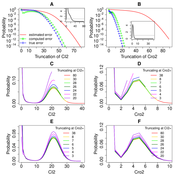
Figure 6: Error quantification and comparisons for the phage lambda bistable epigenetic switch model. (A) and (B): The a priori estimated error (red solid lines), the computed error (green lines and circles), and the true error (blue lines and crosses) of the steady state probability landscapes of $CI$ and $Cro$ dimers at different sizes of truncations. The insets in (A) and (B) show the ratio of the true errors to the computed errors at different sizes of the MEG, and the grey straight line marks the ratio one. The computed errors are larger than the true errors when the black line is below the grey straight line. (C) and (D): The steady state probability landscapes of $CI$ and $Cro$ dimers solved using different truncations of net molecular number in the MEG₁ and MEG₂, respectively. Note that probability distributions end at where truncation occurs. The probabilities in the landscapes are significantly inflated when truncating the state space at smaller net molecular numbers of the corresponding MEG. (E) and (F): The steady state probability landscapes of $CI$ and $Cro$ dimers solved using different truncations of net molecular number in the MEG₂ and MEG₁, respectively. The probabilities in the landscapes are also significantly inflated when truncating the state space at smaller net molecular numbers of the opposite MEG.

These are general formula for upper and lower bounds of the boundary probabilities of any MEG in a reaction network. Note that while $\overline{\tilde{\pi}}^{(N)}_{N}$ is easy to compute, it may not be a tight error bound when the MEG involves many molecular species with overall complex interactions. This will be shown in the example of the phage lambda epigenetic switch model (Fig. 6A and B).

For a reaction network with multiple MEGs, we have

$$\sum_{i=1}^{w}\underline{\tilde{\pi}}^{(N_{i})}_{N_{i}}\leq\sum_{i=1}^{w}\tilde{\pi}^{(N_{i})}_{N_{i}}\leq\sum_{i=1}^{w}\overline{\tilde{\pi}}^{(N_{i})}_{N_{i}},$$

where $N_{i}$ is the maximum copy number for the $i$-th MEG. The upper bounds for the total error $\operatorname{Err}^{(\Omega^{(\mathcal{B})})}$ can therefore be obtained straightforwardly by taking summation of upper bounds for each individual MEG:

$$\operatorname{Err}^{(\Omega^{(\mathcal{B})})}\leq\sum_{i=1}^{w}\overline{\tilde{\pi}}^{(N_{i})}_{N_{i}},$$ (26)

This upper bound of $\sum_{i=1}^{w}\overline{\tilde{\pi}}^{(N_{i})}_{N_{i}}$ can therefore be used as an a priori estimated bound for the total truncation error $\operatorname{Err}^{(\Omega^{(\mathcal{B})})}$ for the state space $\Omega^{(\mathcal{B})}$ using truncation of $\mathcal{B}=(N_{1},\cdots,N_{i},\cdots,N_{j},\cdots,N_{w})$.

Biological Examples

Below we give examples on characterizing the truncation errors in the steady state probability landscapes for four biological reaction networks. We study the models of the birth and death process, the single gene expression, the model of genetic toggle switch, and the phage lambda epigenetic switch model. We first show how each network can be partitioned into MEGs, and how truncation errors for each MEG can be estimated a priori. By enumerating the state space and directly computing the steady state probability landscapes of the dCMEs using the fb-dCME method, we examine the true truncation errors, the computed boundary probabilities, and the a priori estimated truncation error. We demonstrate that indeed the truncation error is bounded from above by the computed boundary probability, and by the a priori error estimate according to theoretical analyses described earlier, once the copy number limit is sufficiently large for the MEG(s).

Birth-Death Process

The birth-death process is a ubiquitous biochemical phenomenon. In its simplest form, it involves synthesis and degradation of only one molecular species. We study this simple birth-death process, whose reaction scheme and rate constants are specified as follows:

$$\begin{split}&R_{1}:\quad\emptyset\stackrel{{\scriptstyle k_{s}}}{{\rightarrow}}X,\quad k_{s}=1/s,\\ &R_{2}:\quad X\stackrel{{\scriptstyle k_{d}}}{{\rightarrow}}\emptyset,\quad k_{d}=0.025/s.\\ \end{split}$$ (27)

The steady state probability landscape of the birth-death process is well known [13, 15]. This process has also been studied extensively as a problem of estimating rare event probability [38, 39, 40].

Molecular equivalent group (MEG).

This single birth and death process is an open network because of the presence of the synthesis reaction. There is only one molecular equivalent group (MEG). We truncate the state space at different values of the maximum copy number of the MEG, ranging from $0$ to $200$, and compute the boundary probabilities at each different truncation.

Asymptotic convergence of errors (Theorem 1).

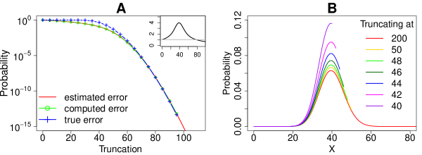
Figure 3: Error quantification and comparisons for the birth-death model. (A): The a priori estimated error (red solid line), the computed error (green line and circles), and the true error (blue line and crosses) of the steady state probability landscape. The inset shows the ratio of the true errors to the computed errors at different sizes of the MEG, and the grey straight line marks the ratio one. The computed errors are larger than the true errors when the black line is below the grey straight line. (B): The steady state probability landscapes of $X$ obtained with different truncations of net molecular number in the MEG. Note that probability distributions end at $X$ where truncation occurs. The probabilities in the landscapes are inflated when truncating the state space at smaller net molecular numbers of the MEG.

To numerically demonstrate Theorem 1, we compute the true truncation error of the steady state solution to the dCME. We use a large copy number of $MEG=200$, which gives an infinitesimally small boundary probability of $1.391\times 10^{-72}$. Steady state solution obtained using this MEG number coincides with analytical solution, and is therefore considered to be exact. With this exact steady state probability landscape, the true truncation error $\operatorname{Err}^{(N)}$ at smaller MEG sizes can be computed using Eqn. (14) (Fig. 3A, blue dashed line and crosses). The corresponding boundary probabilities $\pi^{(\infty)}_{N}$ are computed from this exact steady state probability landscape (Fig. 3A, green dashed line and circles).

Consistent with the statement in the Theorem 1, we find here that the true error $\operatorname{Err}^{(N)}$ (Fig. 3A, blue dashed line and crosses) is bounded by the computed boundary probability $\pi^{(\infty)}_{N}$ (Fig. 3A, green dashed line and circles) when the size of the MEG is sufficiently large. The inset of Fig. 3A shows the ratio of the true errors to the computed errors at different sizes of the MEG, and the grey straight line marks the ratio one. The computed errors are larger than the true errors when the black line is below the grey straight line (Fig. 3A inset). In this example, the computed boundary probability is greater than the true error when $N>79$, as would be expected from Theorem 1.

A priori estimated error bound.

To examine the a priori estimated upper bound for truncation error, we follow Eqn. (22) and (23) to assign values of $\overline{\alpha}_{i}=k_{s}$ and $\underline{\beta}_{i+1}=k_{d}(i+1)$ for this network. We compute the a priori upper error bound for different truncations using Eqn. (24) (Fig. 3A, red solid line). For this simple network, $\overline{\alpha}_{i}=\alpha_{i}=\underline{\alpha}_{i}$ and $\overline{\beta}_{i}=\beta_{i}=\underline{\beta}_{i}$, therefore the a priori estimated error is exactly the same as the analytic solution for the steady state distribution for this simple birth-death network, and it coincides with the computed error (Fig. 3A red and green lines). The true error, computed error, and the a priori error bound all decrease monotonically with increasing MEG size $N$ (Fig. 3A).

Increased probability after state space truncation (Theorem 2).

According to Theorem 2, the probability of a state increases upon state space truncation. We compare the steady state probability landscapes of $X$ computed using truncations at different sizes ranging from 40 to 50 with the exact steady state landscape (Fig. 3B, red line). Our results indeed show clearly that all probabilities increase as more states are truncated (Fig. 3B). The probability landscape computed using $N=50$ (Fig. 3B, yellow line) or larger is very close to the exact landscape using $N=200$ (Fig. 3B, red line). However, the probability landscapes computed using smaller $N$ deviate significantly from the exact probability landscape. The smaller the MEG size, the more significant the deviation is. These results are fully consistent with the statements of Theorem 2.

Single Gene Expression Model

Transcription and translation are fundamental processes in gene regulatory networks that often involve significant stochasticity. The abundance of mRNA and expressed proteins of a gene is usually 2–4 orders of magnitude apart in a cell. There are only a few or dozens of copies of mRNA molecules in each cell for one gene, but the copy number of proteins can range from hundreds to ten thousands [41]. Here we study a model of the fundamental process of single gene transcription and translation using the following reaction scheme and rate constants:

$$\begin{split}&R_{1}:\quad Gene+\emptyset\stackrel{{\scriptstyle k_{e}}}{{\rightarrow}}Gene+mRNA,\quad k_{e}=1.0/s,\\ &R_{2}:\quad mRNA+\emptyset\stackrel{{\scriptstyle k_{t}}}{{\rightarrow}}mRNA+Protein,\quad k_{t}=1.0/s.\\ &R_{3}:\quad mRNA\stackrel{{\scriptstyle k_{m}}}{{\rightarrow}}\emptyset,\quad k_{m}=0.1/s.\\ &R_{4}:\quad Protein\stackrel{{\scriptstyle k_{d}}}{{\rightarrow}}\emptyset,\quad k_{d}=0.01/s.\\ \end{split}$$ (28)

Molecular equivalent group (MEG).

This single gene expression model is an open network. We can participate this model into two molecular equivalent groups (MEG), with MEG₁ consists of species $mRNA$, MEG₂ consists of $Protein$. Note that protein synthesis depends on the copy number $mRNA$, despite the fact that $mRNA$ and $Protein$ are two independent molecular species that cannot be transformed into each other.

Asymptotic convergence of errors (Theorem 1).

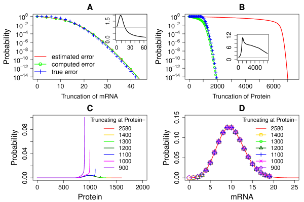
Figure 4: Error quantification and comparisons for the single gene expression model. (A) and (B): The a priori estimated error (red solid lines), the computed error (green lines and circles), and the true error (blue lines and crosses) of the steady state probability landscapes of $mRNA$ and $Protein$ at different sizes of truncations. The insets in (A) and (B) show the ratio of the true errors to the computed errors at different sizes of the MEG, and the grey straight line marks the ratio one. The computed errors are larger than the true errors when the black line is below the grey straight line. (C): The steady state probability landscapes of $Protein$ solved using different truncations of net molecular number in the MEG₂. Note that probability distributions end at where truncation occurs. The probabilities in the landscapes are significantly inflated when truncating the state space at smaller net molecular numbers of the corresponding MEG. (D): The steady state probability landscapes of $mRNA$ solved using different truncations of net molecular number in the MEG₂. In this cases, the probabilities in the landscapes are not affected by the truncation of the opposite MEG.

To numerically demonstrate Theorem 1, we compute the true error of the steady state solution to the dCME using sufficiently large sizes of $MEG_{1}=64$ and $MEG_{2}=2,580$, which gives negligible truncation error, with infinitesimally small boundary probabilities $3.58\times 10^{-30}$ for $MEG_{1}$ and $1.15\times 10^{-32}$ for $MEG_{2}$. Solution obtained using these MEGs is therefore considered to be exact. With this exact steady state probability landscape, the true truncation error $\operatorname{Err}^{(N)}$ at smaller sizes of $MEG_{1}$ and $MEG_{2}$ can be computed using Eqn. (14) (Fig. 4A and B, blue dashed lines and crosses). The corresponding boundary probabilities $\pi^{(\infty)}_{N}$ or computed error are obtained from the exact steady state probability landscape for both $MEG_{1}$ (Fig. 4A, green dashed line and circles) and $MEG_{2}$ (Fig. 4B, green dashed line and circles).

Consistent with the statement in Theorem 1, our results show that the true error $\operatorname{Err}^{(N)}$ is bounded by the computed boundary probability $\pi^{(\infty)}_{N}$ in the $MEG_{1}$ when $N_{1}\geq 20$ (Fig. 4A, blue dashed lines and crosses, green dashed lines and circles, and the inset). In the $MEG_{2}$, although the true errors are larger than computed errors even when the MEG size is large (Fig. 4A inset), the true error can be bounded by the computed error when $N_{2}\geq 5000$ by a multiplication factor of 6 (Fig. 4B, blue dashed lines and crosses, green dashed lines and circles, and the inset). This is expected from Theorem 1.

A priori estimated error bound.

To examine a priori estimated upper bounds for the truncation errors in MEG₁ and MEG₂, we follow Eqn. (22) and (23) to assign values of $\overline{\alpha}_{i}=k_{e}$ and $\underline{\beta}_{(i+1)}=k_{m}(i+1)$ for the $MEG_{1}$. Because of the dependency of protein synthesis on the mRNA copy numbers, we set $\overline{\alpha}_{i}=64\cdot k_{t}$ and $\underline{\beta}_{i+1}=k_{d}(i+1)$ following Eqn. (22) and (23) for the $MEG_{2}$, where the factor $64$ is the maximum copy number of mRNA in the $MEG_{1}$. We compute the a priori estimated upper bounds of errors for different truncations of MEG₁ and MEG₂ using Eqn. (24) (Fig. 4A and B, red solid lines). The true truncation errors and the a priori estimated error bounds of MEG₁ and MEG₂ all decrease monotonically with increasing MEG sizes (Fig. 4A and B). The computed errors also monotonically decrease in both MEGs. For $MEG_{1}$, the a priori estimated error bounds coincide with the computed errors (Fig. 4A red and green lines). For the $MEG_{2}$, the a priori estimated error bounds are larger than computed errors at all MEG sizes.

Increased probability after state space truncation (Theorem 2).

According to Theorem 2, the probability landscape projected on the MEGs increase after state space truncation. We compute the steady state probability landscapes of $Protein$ obtained using truncations at different sizes of the MEG, ranging from $0$ to $2,580$ for $MEG_{2}$ while $MEG_{1}$ is fixed at 64 (Fig. 4C). The results are compared with the exact steady state landscape computed using $MEG_{2}=2,600$ (Fig. 4C, red line).

Our results show clearly that all probabilities in the landscapes increase when more states are truncated at smaller MEG size (Fig. 4C). The probability landscapes computed using larger size of the MEG (e.g., $MEG_{2}=1400$, Fig. 4C, yellow line) are approaching the exact landscape (Fig. 4C, red line). The probability landscapes obtained using smaller MEG sizes deviate significantly from the exact probability landscape. The smaller the MEG size, the more pronounced the deviation is. These numerical results are fully consistent with Theorem 2.

Truncating additional MEGs does not decrease probabilities (Theorem 3).

We further examine Theorem 3, i.e., the probability landscape projected on one MEG increase with state space truncation at another MEG. We compare the projected steady state probability landscapes on $mRNA$ obtained using truncations of different sizes of $MEG_{2}$ ranging from $0$ to $2580$ while the $MEG_{1}$ is fixed at 64 (Fig. 4D). We compare the results with the exact steady state landscape (Fig. 4D, red line).

Our results show that all probabilities on the landscapes of $mRNA$ are not affected by the truncations at the $MEG_{2}$ (Fig. 4D). The probability landscapes computed using different sizes of $MEG_{2}$ are the same (Fig. 4D). These numerical results are completely consistent with Theorem 3, because the probabilities of $mRNA$ are not decreased by the truncation at the MEG of $Protein$.

Genetic Toggle Switch

The bistable genetic toggle switch consists of two genes repressing each other through binding of their protein dimeric products on the promoter sites of the other genes. This genetic network has been studied extensively [42, 43, 44, 45]. We follow references [45, 24] and study a detailed model of the genetic toggle switch with a more realistic control mechanism of gene regulations. Different from simpler toggle switch models [46, 47, 48, 49], in which gene binding and unbinding reactions are approximated by Hill functions, here details of the gene binding and unbinding reactions are modeled explicitly. The molecular species, reactions, and their rate constants are listed below:

$$\begin{split}&R_{1}:GeneA\stackrel{{\scriptstyle k_{1}}}{{\rightarrow}}GeneA+A,\quad k_{sA}=40\,s^{-1}\\ &R_{2}:GeneB\stackrel{{\scriptstyle k_{2}}}{{\rightarrow}}GeneB+B,\quad k_{sB}=20\,s^{-1}\\ &R_{3}:A\stackrel{{\scriptstyle k_{3}}}{{\rightarrow}}\emptyset,\quad k_{dA}=1\,s^{-1}\\ &R_{4}:B\stackrel{{\scriptstyle k_{4}}}{{\rightarrow}}\emptyset,\quad k_{dB}=1\,s^{-1}\\ &R_{5}:2A+GeneB\stackrel{{\scriptstyle k_{5}}}{{\rightarrow}}bGeneB,\quad k_{bA}=1\times 10^{-5}\,nM^{-2}\cdot s^{-1}\\ &R_{6}:2B+GeneA\stackrel{{\scriptstyle k_{6}}}{{\rightarrow}}bGeneA,\quad k_{bB}=3.5\times 10^{-5}\,nM^{-2}\cdot s^{-1}\\ &R_{7}:bGeneB\stackrel{{\scriptstyle k_{7}}}{{\rightarrow}}2A+GeneB,\quad k_{uA}=1\,s^{-1}\\ &R_{8}:bGeneA\stackrel{{\scriptstyle k_{8}}}{{\rightarrow}}2B+GeneA,\quad k_{uB}=1\,s^{-1}\\ \end{split}$$ (29)

Specifically, two genes $GeneA$ and $GeneB$ express protein products $A$ and $B$, respectively. Two protein monomers $A$ or $B$ can bind on the promoter site of $GeneB$ or $GeneA$ to form protein-DNA complexes $bGeneB$ or $bGeneA$, and turn off the expression of $GeneB$ or $GeneA$, respectively.

Molecular equivalent group (MEG).

There are two MEGs in this network, MEG₁ consists of species $A$ and $bGeneB$, MEG₂ consists of $B$ and $bGeneA$.

Asymptotic convergence of errors (Theorem 1).

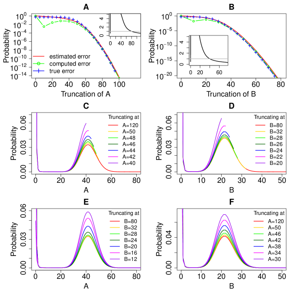
Figure 5: Error quantification and comparisons for the genetic toggle switch model. (A) and (B): The a priori estimated error (red solid lines), the computed error (green lines and circles), and the true error (blue lines and crosses) of the steady state probability landscapes of $A$ and $B$ at different sizes of truncations. The insets in (A) and (B) show the ratio of the true errors to the computed errors at different sizes of the MEG, and the grey straight line marks the ratio one. The computed errors are larger than the true errors when the black line is below the grey straight line. (C) and (D): The steady state probability landscapes of $A$ and $B$ solved using different truncations of net molecular number in the MEG₁ and MEG₂, respectively. Note that probability distributions end at where truncation occurs. The probabilities in the landscapes are significantly inflated when truncating the state space at smaller net molecular numbers of the corresponding MEG. (E) and (F): The steady state probability landscapes of $A$ and $B$ solved using different truncations of net molecular number in the MEG₂ and MEG₁, respectively. The probabilities in the landscapes are also significantly inflated when truncating the state space at smaller net molecular numbers of the opposite MEG.

To numerically demonstrate Theorem 1, we compute the true error of the steady state solution to the dCME using sufficiently large sizes of $MEG_{1}=120$ and $MEG_{2}=80$, which gives negligible truncation error, with infinitesimally small boundary probabilities $5.275\times 10^{-24}$ for $MEG_{1}$ and $2.561\times 10^{-23}$ for $MEG_{2}$. Solution obtained using these MEGs is therefore considered to be exact. With this exact steady state probability landscape, the true truncation error $\operatorname{Err}^{(N)}$ at smaller sizes of $MEG_{1}$ and $MEG_{2}$ can both be computed using Eqn. (14) (Fig. 5A and B, blue dashed lines and crosses). The corresponding boundary probabilities $\pi^{(\infty)}_{N}$ or computed error are computed from the exact steady state probability landscape for both $MEG_{1}$ (Fig. 5A, green dashed line and circles) and $MEG_{2}$ (Fig. 5B, green dashed line and circles).

Consistent with the statement in Theorem 1, our results show that the true error $\operatorname{Err}^{(N)}$ (Fig. 5A and B, blue dashed lines and crosses) is bounded by the computed boundary probability $\pi^{(\infty)}_{N}$ (Fig. 5A and B, green dashed lines and circles) when the size of the MEG is sufficiently large. The insets in Fig. 5A and B show the ratios of the true errors to the computed errors at different sizes of the MEG, and the grey straight line marks the ratio one. The computed errors are larger than the true errors when the black line is below the grey straight line (Fig. 5A and B, insets). In this example, the computed boundary probability is greater than the true error when $MEG_{1}>82$ and $MEG_{2}>42$, as would be expected from Theorem 1.

A priori estimated error bound.

To examine a priori estimated upper bounds for the truncation errors in MEG₁ and MEG₂, we follow Eqn. (22) and (23) to assign values of $\overline{\alpha}_{i}=k_{sA}$ and $\underline{\beta}_{(i+1)}=[(i+1)-2]\cdot k_{dA}$ for the $MEG_{1}$, where the subscript $(i+1)$ is the total copy number of species $A$ in the system. The subtraction of $2$ is necessary because up to $2$ copies of $A$ can be protected from degradation by binding to $GeneB$. This corresponds to the extreme case when $GeneA$ is constantly turned on and $GeneB$ is constantly turned off. Similarly, we have $\overline{\alpha}_{i}=k_{sB}$ and $\underline{\beta}_{i+1}=[(i+1)-2]\cdot k_{dB}$ following Eqn. (22) and (23) for the $MEG_{2}$. This corresponds to the other extreme case when the $GeneB$ is constantly turned on, and $GeneA$ is constantly turned off. We compute the a priori estimated upper bounds of errors for different truncations of MEG₁ and MEG₂ using Eqn. (24) (Fig. 5A and B, red solid lines). The true truncation errors and the a priori estimated error bounds of MEG₁ and MEG₂ all decrease monotonically with increasing MEG sizes (Fig. 5A and B). The computed errors also monotonically decrease when the MEG sizes are larger than $40$ for MEG₁ and $20$ for MEG₂. For both MEGs, the a priori estimated error bounds are larger than computed errors at all MEG sizes. They are also larger than the true errors when the MEG sizes are sufficiently large.

Increased probability after state space truncation (Theorem 2).

According to Theorem 2, the probability landscape projected on the MEGs increase after state space truncation. We first compute the steady state probability landscapes of $A$ obtained using truncations at different sizes of the MEG ranging from $0$ to $119$ for $MEG_{1}$ while $MEG_{2}$ is fixed at 80 (Fig. 5C). The results are compared with the exact steady state landscape computed using $MEG_{1}=120$ and $MEG_{2}=80$ (Fig. 5C, red line). We then also similarly examine the steady state probability landscapes of $B$ obtained using truncations at different sizes of $MEG_{2}$ from $0$ to $79$ while $MEG_{1}$ is fixed at 120 (Fig. 5D).

Our results show clearly that all probabilities in the landscapes increase when more states are truncated at smaller MEG sizes (Fig. 5C and D). The probability landscapes computed using larger sizes of MEGs (e.g., $MEG_{1}=50$, Fig. 5C, yellow line and $MEG_{2}=32$, Fig. 5D, yellow line) are approaching the exact landscape (Fig. 5C and D, red line). The probability landscapes obtained using smaller MEGs deviate significantly from the exact probability landscape. The smaller the MEG size, the more significant the deviation is. These numerical results are completely consistent with Theorem 2.

Truncating additional MEGs does not decrease probabilities (Theorem 3).

We further examine Theorem 3, i.e., the probability landscape projected on one MEG increase with state space truncation at another MEG. We first compare the projected steady state probability landscapes on $A$ obtained using truncations of different sizes of MEGs ranging from $0$ to $80$ for $MEG_{2}$ while $MEG_{1}$ is fixed at 120 (Fig. 5E) We compare the results with the exact steady state landscape (Fig. 5E, red line). We also similarly examine the projected steady state probability landscapes of $B$ obtained using truncations at different sizes of $MEG_{1}$ ranging from $0$ to $120$ while $MEG_{2}$ is fixed at 80 (Fig. 5F).

Our results clearly show that all probabilities on the landscapes of $MEG_{1}$ ($MEG_{2}$) increase when the state space is truncated at $MEG_{2}$ ($MEG_{1}$) (Fig. 5E and F). The probability landscapes computed using larger sizes of MEGs (e.g., $MEG_{2}=32$ in Fig. 5E, yellow line and $MEG_{1}=50$ in Fig. 5F, yellow line) are approaching the exact landscape using $MEG_{1}=120$ and $MEG_{2}=80$ (Fig. 5E and F, red line). However, the probability landscapes using smaller MEGs significantly deviate from the exact probability landscape. The smaller the MEG size, the more significant the deviation is. These numerical results are completely consistent with Theorem 3.

Phage Lambda Bistable Epigenetic Switch

The bistable epigenetic switch for lysogenic maintenance and lytic induction in phage lambda is one of the well-parameterized realistic gene regulatory system. The efficiency and stability of the switch have been extensively studied [50, 51, 52, 53, 54]. Here we characterize the truncation error to the dCME solutions of the reaction network adapted from Cao et al. [5]. The network consists of $11$ different species and $50$ different reactions. The detailed reaction schemes and rate constants are shown in Table 1.

Molecular equivalent group (MEG).

The network can be partitioned into two MEGs. The MEG₁ consists of the dimer of CI protein $CI2$ and all complexes of operator sites bounded with $CI2$. The MEG₂ consists of the dimer of Cro protein $Cro2$ and all complexes of operator sites bounded with $Cro2$.

Asymptotic convergence of errors (Theorem 1).

To numerically demonstrate Theorem 1, we compute the true error of the steady state solution to the dCME using sufficiently large sizes of $MEG_{1}=80$ and $MEG_{2}=38$, which gives negligible truncation error, with infinitesimally small boundary probabilities $6.96\times 10^{-31}$ for $MEG_{1}$ and $3.95\times 10^{-32}$ for $MEG_{2}$. Solution obtained using these MEGs is therefore considered to be exact. With this exact steady state probability landscape, the true truncation error $\operatorname{Err}^{(N)}$ at smaller sizes of $MEG_{1}$ and $MEG_{2}$ can both be computed using Eqn. (14) (Fig. 6A and B, blue dashed lines and crosses). The corresponding boundary probabilities $\pi^{(\infty)}_{N}$ or computed error are computed from the exact steady state probability landscape for both $MEG_{1}$ (Fig. 6A, green dashed line and circles) and $MEG_{2}$ (Fig. 6B, green dashed line and circles).

Consistent with the statement in Theorem 1, our results show that the true error $\operatorname{Err}^{(N)}$ (Fig. 6A and B, blue dashed lines and crosses) is bounded by the computed boundary probability $\pi^{(\infty)}_{N}$ (Fig. 6A and B, green dashed lines and circles) when the size of the MEG is sufficiently large. The insets in Fig. 6A and B show the ratios of the true errors to the computed errors at different sizes of the MEG, and the grey straight lines mark the ratio one. The computed errors are larger than the true errors when the black line is below the grey straight line (Fig. 6A and B, insets). In this example, the computed boundary probability is greater than the true error when $MEG_{1}\geq 24$ and $MEG_{2}\geq 3$, as would be expected from Theorem 1.

A priori estimated error bound.

To examine a priori estimated upper bounds for the truncation errors in MEG₁ and MEG₂, we follow Eqn. (22) and (23) to assign values of $\overline{\alpha}_{i}=k_{s1CI_{2}}$ and $\underline{\beta}_{(i+1)}=[(i+1)-3]\cdot k_{dCI_{2}}$ for the $MEG_{1}$, where the subscript $(i+1)$ is the total copy number of species $CI2$ in the system. The subtraction of $3$ is necessary because up to $3$ copies of $CI2$ can be protected from degradation by binding to operator sites $OR1$, $OR2$, and $OR3$. Similarly, we have $\overline{\alpha}_{i}=k_{sCro_{2}}$ and $\underline{\beta}_{i+1}=[(i+1)-3]\cdot k_{dCro_{2}}$ following Eqn. (22) and (23) for the $MEG_{2}$. We compute the a priori estimated upper bounds of errors for different truncations of MEG₁ and MEG₂ using Eqn. (24) (Fig. 6A and B, red solid lines). The true truncation errors and the a priori estimated error bounds of MEG₁ and MEG₂ all decrease monotonically with increasing MEG sizes (Fig. 6A and B). The computed errors also monotonically decrease when the MEG sizes are larger than $13$ for MEG₁ and $4$ for MEG₂. For both MEGs, the a priori estimated error bounds are larger than computed errors at all MEG sizes. They are also larger than the true errors when the MEG sizes are sufficiently large.

Increased probability after state space truncation (Theorem 2).

According to Theorem 2, the probability landscape projected on the MEGs increase after state space truncation. We first compute the steady state probability landscapes of $CI2$ obtained by truncating $MEG_{1}$ at different sizes ranging from $0$ to $80$ while $MEG_{2}$ is fixed at $38$ (Fig. 6C). The results are compared with the exact steady state landscape computed using $MEG_{1}=80$ and $MEG_{2}=38$ (Fig. 6C, red line). We then also similarly examine the steady state probability landscapes of $Cro2$ obtained by truncating at different sizes of $MEG_{2}$ from $0$ to $38$ while $MEG_{1}$ is fixed at $80$ (Fig. 6D).

Our results show clearly that all probabilities in the landscapes increase when more states are truncated at smaller MEG sizes (Fig. 6C and D). The probability landscapes computed using larger sizes of MEGs (e.g., $MEG_{1}=30$, Fig. 6C, yellow line and $MEG_{2}=8$, Fig. 6D, yellow line) are approaching the exact landscape (Fig. 6C and D, red line). The probability landscapes obtained using smaller MEGs deviate significantly from the exact probability landscape. The smaller the MEG size, the more significant the deviation is. These numerical results are completely consistent with Theorem 2.

Truncating additional MEGs does not decrease probabilities (Theorem 3).

We further examine Theorem 3, i.e., the probability landscape projected on one MEG increase with state space truncation at another MEG. We first compare the projected steady state probability landscapes on $CI2$ obtained by truncating $MEG_{2}$ at different sizes ranging from $0$ to $38$ while $MEG_{1}$ is fixed at $80$ (Fig. 6E). We compare the results with the exact steady state landscape (Fig. 6E, red line). We also similarly examine the projected steady state probability landscapes of $Cro2$ obtained by truncating at different sizes of $MEG_{1}$ ranging from $0$ to $80$ while $MEG_{2}$ is fixed at $38$ (Fig. 6F).

Our results show that all probabilities on the landscapes of $MEG_{1}$ ($MEG_{2}$) increase when the state space is truncated at $MEG_{2}$ ($MEG_{1}$) (Fig. 6E and F). The probability landscapes computed using larger sizes of MEGs (e.g., $MEG_{2}=8$ in Fig. 6E, yellow line and $MEG_{1}=30$ in Fig. 6F, yellow line) are approaching the exact landscape using $MEG_{1}=80$ and $MEG_{2}=38$ (Fig. 6E and F, red line). However, the probability landscapes using smaller MEGs significantly deviate from the exact probability landscape. The smaller the MEG size, the more significant the deviation is. These numerical results are completely consistent with Theorem 3.

Discussions and Conclusions

Solving the discrete chemical master equation (dCME) is of fundamental importance for studying stochasticity in reaction networks. The main challenges are the discrete nature of the states and the difficulty in enumerating these states, as the size of the state space expands rapidly when the network becomes more complex. In this study, we describe a novel approach for state space truncation. Instead of taking a high dimensional hypercube as the truncated state space, we introduce the concept of molecular equivalence group (MEG), and truncate the state space into the same or lower dimensional simplexes, with the same effective copy number of molecules in each dimension by taking advantage of the principle of mass conservation. For complex networks, the reduction of the size of the state space can be dramatic.

Our study addresses a key issue in obtaining direct solution to the dCME. As state space truncation is inevitable, it is important to quantify the errors of such truncations, so the accuracy of the dCME solutions can be assessed and managed. We have developed a general theoretical framework for quantifying the errors of state space truncation on the steady state probability landscape. By decomposing the reaction network into MEGs, the error contribution from each individual MEG is quantified. This critically important task is made possible through analyzing the states on the reflecting boundary and their associated steady state probabilities. The boundary probability analysis has been based on the construction of an aggregated continuous-time Markov process by factoring the state space according to the total numbers of molecules in each MEG. With explicit formulas for calculating conservative error bounds for the steady state, one can easily calculate the a priori error bounds for any given size of a MEG. Furthermore, our theory allows the determination of the minimally required sizes of MEGs if a predefined error tolerance is to be satisfied. As shown in the examples, to determine the appropriate MEG sizes a priori, one can first calculate the estimated errors at different sizes of each MEG, and choose the minimal MEG sizes that satisfies the overall error tolerance. This eliminates the need of multiple iterations of costly trial computations to solve the dCME for determining the appropriate total copy numbers necessary to ensure small truncation errors. This is advantageous over conventional numerical techniques, where errors are typically assessed through post processing of trial solutions.

In complex networks, state truncation in one molecular group may affect the errors of other molecular groups. By partitioning the network into separate molecular equivalent groups (MEGs), the mutual influence of the effects of state truncations in different groups can be reduced. In such cases, we have proved that the asymptotic errors in any truncated MEG will not be under-estimated by the state truncations in other MEGs. Based on this conclusion, one can increase the size of each particular MEG in order to achieve a small truncation error of that MEG. When the truncation error for every MEG is below the prescribed threshold of error tolerance, the total truncation error of the whole state space will be guaranteed to be bounded by the sum of individual truncation errors in each MEG.

While our method ensures that there is no mass exchange between different MEGs and often couplings between MEGs are weak, it does not rule out the existence of possible strong couplings among MEGs. In the example of the single gene expression model, there is a strong coupling between mass-isolated mRNA MEG and the protein MEG. In this case, protein synthesis strongly depends on the amount of available mRNA. As a result, the protein probability distribution can be heavily influenced by the choices of the mRNA MEG size, and its peak is shifted when the size of mRNA MEG is near exhaustion (data not shown). This issue rapidly disappears when MEG sizes become sufficiently large to ensure that the truncation error to be smaller than the specified error tolerance (Fig. 4).

Our method differs from the finite state projection (FSP) method [23, 30], which employs an absorbing boundary state to calculate the truncation error. Transitions from any states in the available finite state space to any outside state are send to the absorbing state, and the reactions are made irreversible. The truncation error in the FSP method is taken as the probability mass on the absorbing boundary state. It has two components: one from the lost probability mass due to the state truncation, the other from the trapped probability mass due to the absorbing nature of the boundary state. As time proceeds, the trapped probability mass on the absorbing state will grow and dominate. At the steady state, all probability mass will be trapped in the absorbing state, which can no longer reflect the truncated probability mass. Therefore, the FSP method cannot be used to study the long-term as well as the steady state behavior of a stochastic network.

In contrast, our method employs a reflecting boundary and can characterize the truncation errors in the steady state. All transitions between boundary and non-boundary states are retained after state space truncation, and the reversible nature of transitions unaltered. The reflecting boundaries allow analysis of the steady state truncation error of each MEG. Our method can be used to study the steady state probability landscape. Furthermore, our method also allows direct computation of the distribution of first passage time, an important problem in studying rare events in biological networks currently relies heavily on sampling techniques.

We have also provided computational results of four stochastic networks, namely, the birth-death process consisting of one MEG, the single gene expression model, the genetic toggle switch model, and the phage lambda epigenetic switch model, each consisting of two MEGs, respectively. By comparing true errors, computed errors, and a priori estimated errors at different truncation sizes, we have numerically verified the theorems presented in this study: First, the true error for truncating a MEG is bounded by the total probability mass on the reflecting boundary of the MEG (Theorem 1). Second, the projected probability on one MEG increases upon the state space truncation at this MEG (Theorem 2). Third, the projected probability on one MEG also increases when the state space is truncated at another MEG (Theorem 3). Furthermore, we show that the a priori estimated error bound are effective when the network is truncated at a sufficiently large size of MEG.

Recent studies based on tensor representation of the transition rate matrices show that the storage requirement of solving CME can be significantly reduced and computational time improved [49, 55]. However, accurate tensor representation and tensor-based approximation strongly depend on the separability of system states, that is, whether the system can be decomposed into a number of relatively independent smaller sub-systems [56, 49]. While complete separability can be achieved in some cases, e.g. the one-dimensional quantum spin system [56], errors are generally unknown for biological networks that are not fully separable.

The tensor method of Liao et al can reduce the state space dramatically for a number of networks [55]. For example, the size of the state space of the Fokker-Planck equation of the Schlögl model is reduced from $2.74\times 10^{11}$ to $4.01\times 10^{3}+2.07\times 10^{5}$, with a reduction factor of $10^{6}$. It will be interesting to further assess the reduction factor if the full discrete CMEs instead of the Fokker-Planck equations of these network models are solved so a direct comparison can be carried out.

Our finite buffer approach compares favorably with the tensor train method of [49] for the network of enzymatic futile cycles [40]. This network is a closed system and technically no finite buffer is required when the enumerated states can fit into the computer memory, therefore analysis of truncation error would be unnecessary. Regardless, our approach of state enumeration leads to a state space of only $1,071$ microstates, a reflection of the $O(n!)$ order of reduction. In contrast, the tensor train method is based on a state space of a size of $2^{22}=4.19\times 10^{6}$. Using our finite buffer method, both the time-evolving and the steady state probability landscapes can be computed efficiently in $<10$ seconds (data not shown), but the tensor-train method requires $1.52\times 10^{4}$ seconds for the time evolution of $t=1$ to be computed as reported in [49]. For the model of toggle switch, computing the time-evolution of the probability landscape up to $t=30$ seconds requires $14,541$ seconds or 4 hours of wall clock time using the tensor-train method [49]. Our method completes the computation of the steady state probability landscape in ca. $3,300$ seconds or $55$ minutes of wall clock time.

We further note that our work complements tensor-based methods [49, 55]. Tensor-based methods directly reduce the storage of the transition rate matrices [49], without altering the hypercubic nature of the underlying state space. In contrast, our method first reduces the state space by a factor of $O(n!)$, leading to a dramatically reduced transition rate matrix. It is possible that there exist alternative approaches to construct tensors of the transition rate matrix without assuming that the truncated state space is a hypercube as is the case in [49]. Whether our approach can be useful for further reduction of storage and computational speed-up is a possible direction for future exploration.

Overall, we have introduced an efficient method for state space truncation and have developed theory to quantify the errors of state space truncations. Results presented here provide a general framework for high precision numerical solutions to a dCME. It is envisioned that the approach of direct solution of a dCME can be broadly applied to many stochastic reaction networks, such as those found in systems biology and in synthetic biology.

APPENDIX

Proof of Lemma 1

• By sorting the state space according to the partition $\tilde{\Omega}^{(\infty)}$ and re-constructing the transition rate matrix $\tilde{{\mbox{\boldmath$A$}}}$ in Eqn. (6), the dCME can be re-written as $\frac{d\tilde{{\mbox{\boldmath$p$}}}^{(\infty)}(t)}{dt}=\tilde{{\mbox{\boldmath$A$}}}\tilde{{\mbox{\boldmath$p$}}}^{(\infty)}(t)$, where $\tilde{{\mbox{\boldmath$p$}}}^{(\infty)}$ is the probability distribution on the partitioned state space. We sum up the master equations over all microstates in each group $\mathcal{G}_{i}$ and obtain a separate aggregated equation for each group. As the re-ordered matrix $\tilde{{\mbox{\boldmath$A$}}}$ is a block tri-diagonal matrix, the summed discrete chemical master equation is reduced to:

  $$\begin{split}\frac{dp^{(\infty)}(\mathcal{G}_{0},t)}{dt}&=\frac{d\sum_{{\mbox{\boldmath$x$}}\in\mathcal{G}_{0}}p({\mbox{\boldmath$x$}},t)}{dt}=\left(\mathbbm{1}^{T}{\mbox{\boldmath$A$}}_{0,0}\right)\tilde{{\mbox{\boldmath$p$}}}^{(\infty)}(\mathcal{G}_{0},t)+\left(\mathbbm{1}^{T}{\mbox{\boldmath$A$}}_{0,1}\right)\tilde{{\mbox{\boldmath$p$}}}^{(\infty)}(\mathcal{G}_{1},t),\\ \frac{dp^{(\infty)}(\mathcal{G}_{i},t)}{dt}&=\frac{d\sum_{{\mbox{\boldmath$x$}}\in\mathcal{G}_{i}}p({\mbox{\boldmath$x$}},t)}{dt}=\left(\mathbbm{1}^{T}{\mbox{\boldmath$A$}}_{i,i-1}\right)\tilde{{\mbox{\boldmath$p$}}}^{(\infty)}(\mathcal{G}_{i-1},t)+\left(\mathbbm{1}^{T}{\mbox{\boldmath$A$}}_{i,i}\right)\tilde{{\mbox{\boldmath$p$}}}^{(\infty)}(\mathcal{G}_{i},t)+\left(\mathbbm{1}^{T}{\mbox{\boldmath$A$}}_{i,i+1}\right)\tilde{{\mbox{\boldmath$p$}}}^{(\infty)}(\mathcal{G}_{i+1},t),\\ \text{for }i=1,\cdots,\infty.\\ \end{split}$$ (30)

The overall probability change of each group $\mathcal{G}_{i}$ depends on the probability vector $\tilde{{\mbox{\boldmath$p$}}}^{(\infty)}(\mathcal{G}_{i},t)$ itself, as well as the probability vector $\tilde{{\mbox{\boldmath$p$}}}^{(\infty)}(\mathcal{G}_{i-1},t)$ and the probability vector $\tilde{{\mbox{\boldmath$p$}}}^{(\infty)}(\mathcal{G}_{i+1},t)$ of the immediate neighboring groups. It also depends on the rates of synthesis and degradation reactions in elements of ${\mbox{\boldmath$A$}}_{i,i-1}$ and ${\mbox{\boldmath$A$}}_{i,i+1}$, respectively, as well as rates of coupling reactions in ${\mbox{\boldmath$A$}}_{i,i}$. From the definition of transition rate matrix given in Eqn. (3), we have:

$$\begin{split}\mathbbm{1}^{T}{\mbox{\boldmath$A$}}_{0,0}&=-\mathbbm{1}^{T}{\mbox{\boldmath$A$}}_{1,0},\\ \mathbbm{1}^{T}{\mbox{\boldmath$A$}}_{i-1,i}+\mathbbm{1}^{T}{\mbox{\boldmath$A$}}_{i,i}&=-\mathbbm{1}^{T}{\mbox{\boldmath$A$}}_{i+1,i},\quad\text{for }i=1,\cdots,\infty.\\ \end{split}$$ (31)

At the steady state when all $\frac{dp^{(\infty)}(\mathcal{G}_{i})}{dt}=0$, we combine line 1 of Eqn. (30) and line 1 of Eqn. (31), and obtain:

$$\left(\mathbbm{1}^{T}{\mbox{\boldmath$A$}}_{1,0}\right)\tilde{{\mbox{\boldmath$\pi$}}}^{(\infty)}(\mathcal{G}_{0})=\left(\mathbbm{1}^{T}{\mbox{\boldmath$A$}}_{0,1}\right)\tilde{{\mbox{\boldmath$\pi$}}}^{(\infty)}(\mathcal{G}_{1}).$$

From line 2 of Eqn. (30) at steady state and after incorporating line 1 of Eqn. (31), we have: $\left(\mathbbm{1}^{T}{\mbox{\boldmath$A$}}_{1,2}\right)\tilde{{\mbox{\boldmath$\pi$}}}^{(\infty)}(\mathcal{G}_{2})=\left(\mathbbm{1}^{T}{\mbox{\boldmath$A$}}_{0,0}\right)\tilde{{\mbox{\boldmath$\pi$}}}^{(\infty)}(\mathcal{G}_{0})-\left(\mathbbm{1}^{T}{\mbox{\boldmath$A$}}_{1,1}\right)\tilde{{\mbox{\boldmath$\pi$}}}^{(\infty)}(\mathcal{G}_{1}).$ After further incorporating line 1 of Eqn. (30) at steady state, we have $\left(\mathbbm{1}^{T}{\mbox{\boldmath$A$}}_{1,2}\right)\tilde{{\mbox{\boldmath$\pi$}}}^{(\infty)}(\mathcal{G}_{2})=-\left(\mathbbm{1}^{T}{\mbox{\boldmath$A$}}_{0,1}\right)\tilde{{\mbox{\boldmath$\pi$}}}^{(\infty)}(\mathcal{G}_{1})-\left(\mathbbm{1}^{T}{\mbox{\boldmath$A$}}_{1,1}\right)\tilde{{\mbox{\boldmath$\pi$}}}^{(\infty)}(\mathcal{G}_{1}).$ Incorporating line 2 of Eqn. (31), we have:

$$\left(\mathbbm{1}^{T}{\mbox{\boldmath$A$}}_{2,1}\right)\tilde{{\mbox{\boldmath$\pi$}}}^{(\infty)}(\mathcal{G}_{1})=\left(\mathbbm{1}^{T}{\mbox{\boldmath$A$}}_{1,2}\right)\tilde{{\mbox{\boldmath$\pi$}}}^{(\infty)}(\mathcal{G}_{2}).$$

Assume $\left(\mathbbm{1}^{T}{\mbox{\boldmath$A$}}_{i,\,i-1}\right)\tilde{{\mbox{\boldmath$\pi$}}}^{(\infty)}(\mathcal{G}_{i-1})=\left(\mathbbm{1}^{T}{\mbox{\boldmath$A$}}_{i-1,\,i}\right)\tilde{{\mbox{\boldmath$\pi$}}}^{(\infty)}(\mathcal{G}_{i}),$ we have from the $i$-the line of Eqn. (30) at the steady state

$$\begin{split}\left(\mathbbm{1}^{T}{\mbox{\boldmath$A$}}_{i,\,i+1}\right)\tilde{{\mbox{\boldmath$\pi$}}}^{(\infty)}(\mathcal{G}_{i+1})&=-\left(\mathbbm{1}^{T}{\mbox{\boldmath$A$}}_{i,\,i-1}\right)\tilde{{\mbox{\boldmath$\pi$}}}^{(\infty)}(\mathcal{G}_{i-1})-\left(\mathbbm{1}^{T}{\mbox{\boldmath$A$}}_{i,\,i}\right)\tilde{{\mbox{\boldmath$\pi$}}}^{(\infty)}(\mathcal{G}_{i})\\ &=-\left(\mathbbm{1}^{T}{\mbox{\boldmath$A$}}_{i-1,\,i}\right)\tilde{{\mbox{\boldmath$\pi$}}}^{(\infty)}(\mathcal{G}_{i})-\left(\mathbbm{1}^{T}{\mbox{\boldmath$A$}}_{i,\,i}\right)\tilde{{\mbox{\boldmath$\pi$}}}^{(\infty)}(\mathcal{G}_{i}).\end{split}$$ (32)

With the $i$-th line of Eqn. (31), we further have:

$$\left(\mathbbm{1}^{T}{\mbox{\boldmath$A$}}_{i,\,i+1}\right)\tilde{{\mbox{\boldmath$\pi$}}}^{(\infty)}(\mathcal{G}_{i+1})=\left(\mathbbm{1}^{T}{\mbox{\boldmath$A$}}_{i+1,\,i}\right)\tilde{{\mbox{\boldmath$\pi$}}}^{(\infty)}(\mathcal{G}_{i}).$$

Overall, we have:

$$\begin{split}\left(\mathbbm{1}^{T}{\mbox{\boldmath$A$}}_{1,0}\right)\tilde{{\mbox{\boldmath$\pi$}}}^{(\infty)}(\mathcal{G}_{0})&=\left(\mathbbm{1}^{T}{\mbox{\boldmath$A$}}_{0,1}\right)\tilde{{\mbox{\boldmath$\pi$}}}^{(\infty)}(\mathcal{G}_{1}),\\ \left(\mathbbm{1}^{T}{\mbox{\boldmath$A$}}_{i+1,i}\right)\tilde{{\mbox{\boldmath$\pi$}}}^{(\infty)}(\mathcal{G}_{i})&=\left(\mathbbm{1}^{T}{\mbox{\boldmath$A$}}_{i,i+1}\right)\tilde{{\mbox{\boldmath$\pi$}}}^{(\infty)}(\mathcal{G}_{i+1}),\\ \text{for }i=1,\cdots,\infty.\\ \end{split}$$ (33)

As both sides are constants, we can find $\alpha_{i}$ and $\beta_{i+1}$ such that:

$$\begin{split}\left(\mathbbm{1}^{T}{\mbox{\boldmath$A$}}_{i+1,i}\right)\tilde{{\mbox{\boldmath$\pi$}}}^{(\infty)}(\mathcal{G}_{i})=\mathbbm{1}^{T}\alpha_{i}\tilde{{\mbox{\boldmath$\pi$}}}^{(\infty)}(\mathcal{G}_{i})&=\alpha_{i}\mathbbm{1}^{T}\tilde{{\mbox{\boldmath$\pi$}}}^{(\infty)}(\mathcal{G}_{i}),\\ \left(\mathbbm{1}^{T}{\mbox{\boldmath$A$}}_{i,i+1}\right)\tilde{{\mbox{\boldmath$\pi$}}}^{(\infty)}(\mathcal{G}_{i+1})=\mathbbm{1}^{T}\beta_{i+1}\tilde{{\mbox{\boldmath$\pi$}}}^{(\infty)}(\mathcal{G}_{i+1})&=\beta_{i+1}\mathbbm{1}^{T}\tilde{{\mbox{\boldmath$\pi$}}}^{(\infty)}(\mathcal{G}_{i+1}),\end{split}$$ (34)

for all $i=0,1,\cdots$, where $i$ is the total copy number of the MEG. We obviously have:

$$\alpha_{i}=\left(\mathbbm{1}^{T}{\mbox{\boldmath$A$}}_{i+1,i}\right)\cdot\frac{\tilde{{\mbox{\boldmath$\pi$}}}^{(\infty)}(\mathcal{G}_{i})}{\mathbbm{1}^{T}\tilde{{\mbox{\boldmath$\pi$}}}^{(\infty)}(\mathcal{G}_{i})}\quad\text{and}\quad\beta_{i+1}=\left(\mathbbm{1}^{T}{\mbox{\boldmath$A$}}_{i,i+1}\right)\cdot\frac{\tilde{{\mbox{\boldmath$\pi$}}}^{(\infty)}(\mathcal{G}_{i+1})}{\mathbbm{1}^{T}\tilde{{\mbox{\boldmath$\pi$}}}^{(\infty)}(\mathcal{G}_{i+1})},$$

where $\alpha_{i}$ is the sum of column-sums of sub-matrix ${\mbox{\boldmath$A$}}_{i+1,i}$ weighted by the steady state probability distribution $\tilde{{\mbox{\boldmath$\pi$}}}^{(\infty)}$ on group $\mathcal{G}_{i}$, $\beta_{i+1}$ is the sum of column-summation of sub-matrix ${\mbox{\boldmath$A$}}_{i,i+1}$ weighted by the steady state probability distribution on group $\mathcal{G}_{i+1}$.

As $\mathbbm{1}^{T}\tilde{{\mbox{\boldmath$\pi$}}}^{(\infty)}(\mathcal{G}_{i})$ is the total steady state probability mass over states in group $\mathcal{G}_{i}$, we substitute Eqn. (34) back into Eqn. (33) and obtain the following relationship of steady state distribution on the partitions of $\tilde{\Omega}^{\infty}$:

$$\begin{split}\alpha_{0}\mathbbm{1}^{T}\tilde{{\mbox{\boldmath$\pi$}}}^{(\infty)}(\mathcal{G}_{0})&=\beta_{1}\mathbbm{1}^{T}\tilde{{\mbox{\boldmath$\pi$}}}^{(\infty)}(\mathcal{G}_{1}),\\ \alpha_{i}\mathbbm{1}^{T}\tilde{{\mbox{\boldmath$\pi$}}}^{(\infty)}(\mathcal{G}_{i})&=\beta_{i+1}\mathbbm{1}^{T}\tilde{{\mbox{\boldmath$\pi$}}}^{(\infty)}(\mathcal{G}_{i+1}),\\ \text{for }i=1,\cdots,\infty.\\ \end{split}$$ (35)

The steady state solution to Eqn. (35) is equivalent to the steady state solution of a dCME with the transition rate matrix $B$ defined as in Eqn. (9).

Proof of Lemma 15

• If $\lim_{N\rightarrow\infty}\sup\limits_{i>N}\frac{\alpha^{(\infty)}_{i}}{\beta^{(\infty)}_{i+1}}\geq 1$ held, then there would be an infinite number of terms $\frac{\alpha^{(\infty)}_{i}}{\beta^{(\infty)}_{i+1}}>1$. There should exist an integer $N^{\prime}$ such that for all $i>N^{\prime}$, we have $\beta^{(\infty)}_{i+1}\leq\alpha^{(\infty)}_{i}$. According to Eqn. (35), we would have $\tilde{\pi}^{(\infty)}_{i+1}\geq\tilde{\pi}^{(\infty)}_{i}$ in the steady state for all $i>N^{\prime}$. This contradicts with the assumption of a finite system, as the total probability mass on boundary states increases monotonically as the net molecular copy number of the network increases after $N^{\prime}$. This makes the overall system a pure-birth process. Therefore, for a finite biological system, we have Eqn. (15).

Proof of Theorem 1

• From Eqn. (13), we can first derive an explicit expression of the true error $\operatorname{Err}^{(N)}$ using the aggregated synthesis and degradation rates $\alpha^{(\infty)}_{k}$ and $\beta^{(\infty)}_{k+1}$ given in Eqn. (8):

  $$\operatorname{Err}^{(N)} =1-\sum_{{\mbox{\boldmath$x$}}\in\Omega^{(N)}}\pi^{(\infty)}({\mbox{\boldmath$x$}})=1-\sum_{i=0}^{N}\mathbbm{1}^{T}\tilde{{\mbox{\boldmath$\pi$}}}^{(\infty)}(\mathcal{G}_{i})=1-\tilde{\pi}_{0}^{(\infty)}(1+\sum_{j=1}^{N}\prod_{k=0}^{j-1}\frac{\alpha^{(\infty)}_{k}}{\beta^{(\infty)}_{k+1}})$$ (36)

  $$=1-\frac{1+\sum_{j=1}^{N}\prod_{k=0}^{j-1}\frac{\alpha^{(\infty)}_{k}}{\beta^{(\infty)}_{k+1}}}{1+\sum_{j=1}^{\infty}\prod_{k=0}^{j-1}\frac{\alpha^{(\infty)}_{k}}{\beta^{(\infty)}_{k+1}}}=\frac{\sum_{j=N+1}^{\infty}\prod_{k=0}^{j-1}\frac{\alpha^{(\infty)}_{k}}{\beta^{(\infty)}_{k+1}}}{1+\sum_{j=1}^{\infty}\prod_{k=0}^{j-1}\frac{\alpha^{(\infty)}_{k}}{\beta^{(\infty)}_{k+1}}}$$

  From Eqn. (36), Eqn. (13), and Lemma 15, we have:

  $$\frac{\operatorname{Err}^{(N)}}{\tilde{\pi}^{(\infty)}_{N}} =\frac{\sum_{j=N+1}^{\infty}\prod_{k=0}^{j-1}\frac{\alpha^{(\infty)}_{k}}{\beta^{(\infty)}_{k+1}}}{\prod_{k=0}^{N-1}\frac{\alpha^{(\infty)}_{k}}{\beta^{(\infty)}_{k+1}}}=\frac{(\prod_{k=0}^{N-1}\frac{\alpha^{(\infty)}_{k}}{\beta^{(\infty)}_{k+1}})(\sum_{j=N+1}^{\infty}\prod_{k=N}^{j-1}\frac{\alpha^{(\infty)}_{k}}{\beta^{(\infty)}_{k+1}})}{\prod_{k=0}^{N-1}\frac{\alpha^{(\infty)}_{k}}{\beta^{(\infty)}_{k+1}}}$$ (37)

  $$=\sum_{j=N+1}^{\infty}\prod_{k=N}^{j-1}\frac{\alpha^{(\infty)}_{k}}{\beta^{(\infty)}_{k+1}}\leq\sum_{j=N+1}^{\infty}\left[\sup\limits_{k\geq N}\left\{\frac{\alpha^{(\infty)}_{k}}{\beta^{(\infty)}_{k+1}}\right\}\right]^{j-N}=\sum_{j=1}^{\infty}\left[\sup\limits_{k\geq N}\left\{\frac{\alpha^{(\infty)}_{k}}{\beta^{(\infty)}_{k+1}}\right\}\right]^{j},$$

  When $N$ is sufficiently large, $\sup\limits_{k\geq N}\left\{\frac{\alpha^{(\infty)}_{k}}{\beta^{(\infty)}_{k+1}}\right\}<1$ from Lemma 15, the terms in the infinite series $\sum_{j=1}^{\infty}\left[\sup\limits_{k\geq N}\left\{\frac{\alpha^{(\infty)}_{k}}{\beta^{(\infty)}_{k+1}}\right\}\right]^{j}$ then forms a converging geometric series. Therefore, we have

  $$\sum_{j=1}^{\infty}\left[\sup\limits_{k\geq N}\left\{\frac{\alpha^{(\infty)}_{k}}{\beta^{(\infty)}_{k+1}}\right\}\right]^{j}=\frac{\sup\limits_{k\geq N}\left\{\frac{\alpha^{(\infty)}_{k}}{\beta^{(\infty)}_{k+1}}\right\}}{1-\sup\limits_{k\geq N}\left\{\frac{\alpha^{(\infty)}_{k}}{\beta^{(\infty)}_{k+1}}\right\}},$$

  and the following inequality holds:

  $$\lim_{N\rightarrow\infty}\frac{\operatorname{Err}^{(N)}}{\bar{\pi}^{(\infty)}_{N}}\leq\lim_{N\rightarrow\infty}\frac{\sup\limits_{k\geq N}\left\{\frac{\alpha^{(\infty)}_{k}}{\beta^{(\infty)}_{k+1}}\right\}}{1-\sup\limits_{k\geq N}\left\{\frac{\alpha^{(\infty)}_{k}}{\beta^{(\infty)}_{k+1}}\right\}}.$$

Let $M\in\{N,\cdots,\infty\}$ be the integer such that $\frac{\alpha^{(\infty)}_{M}}{\beta^{(\infty)}_{M+1}}=\mathop{\sup}\limits_{k\geq N}\left\{\frac{\alpha^{(\infty)}_{k}}{\beta^{(\infty)}_{k+1}}\right\}$, we have the following inequality equivalent to Inequality (16):

$$\lim_{N\rightarrow\infty}\frac{\operatorname{Err}^{(N)}}{\bar{\pi}^{(\infty)}_{N}}\leq\lim_{N\rightarrow\infty}\frac{\frac{\alpha^{(\infty)}_{M}}{\beta^{(\infty)}_{M+1}}}{1-\frac{\alpha^{(\infty)}_{M}}{\beta^{(\infty)}_{M+1}}}.$$

Proof of Theorem 2

• We first consider two truncated state spaces $\tilde{\Omega}^{(N)}$ and $\tilde{\Omega}^{(N+1)}$. Following Eqn. (30), two finite sets of the block chemical master equation can be constructed for these two state spaces. The first set containing $N$ equations is built on the state space $\tilde{\Omega}^{(N)}$.

  $$\begin{split}\frac{dp^{(N)}(\mathcal{G}_{0},t)}{dt}&=\left(\mathbbm{1}^{T}{\mbox{\boldmath$A$}}_{0,0}\right)\tilde{{\mbox{\boldmath$p$}}}^{(N)}(\mathcal{G}_{0},t)+\left(\mathbbm{1}^{T}{\mbox{\boldmath$A$}}_{0,1}\right)\tilde{{\mbox{\boldmath$p$}}}^{(N)}(\mathcal{G}_{1},t),\\ \frac{dp^{(N)}(\mathcal{G}_{i},t)}{dt}&=\left(\mathbbm{1}^{T}{\mbox{\boldmath$A$}}_{i,i-1}\right)\tilde{{\mbox{\boldmath$p$}}}^{(N)}(\mathcal{G}_{i-1},t)+\left(\mathbbm{1}^{T}{\mbox{\boldmath$A$}}_{i,i}\right)\tilde{{\mbox{\boldmath$p$}}}^{(N)}(\mathcal{G}_{i},t)+\left(\mathbbm{1}^{T}{\mbox{\boldmath$A$}}_{i,i+1}\right)\tilde{{\mbox{\boldmath$p$}}}^{(N)}(\mathcal{G}_{i+1},t),\\ \text{for }i=1,\cdots,N-1,\\ \frac{dp^{(N)}(\mathcal{G}_{N},t)}{dt}&=\left(\mathbbm{1}^{T}{\mbox{\boldmath$A$}}_{N,N-1}\right)\tilde{{\mbox{\boldmath$p$}}}^{(N)}(\mathcal{G}_{N-1},t)+\left(\mathbbm{1}^{T}{\mbox{\boldmath$A$}}_{N,N}\right)\tilde{{\mbox{\boldmath$p$}}}^{(N)}(\mathcal{G}_{N},t).\\ \end{split}$$ (38)

  The second set is built on the state space $\tilde{\Omega}^{(N+1)}$ containing $N+1$ equations.

  $$\begin{split}\frac{dp^{(N+1)}(\mathcal{G}_{0},t)}{dt}&=\left(\mathbbm{1}^{T}{\mbox{\boldmath$A$}}_{0,0}\right)\tilde{{\mbox{\boldmath$p$}}}^{(N+1)}(\mathcal{G}_{0},t)+\left(\mathbbm{1}^{T}{\mbox{\boldmath$A$}}_{0,1}\right)\tilde{{\mbox{\boldmath$p$}}}^{(N+1)}(\mathcal{G}_{1},t),\\ \frac{dp^{(N+1)}(\mathcal{G}_{i},t)}{dt}&=\left(\mathbbm{1}^{T}{\mbox{\boldmath$A$}}_{i,i-1}\right)\tilde{{\mbox{\boldmath$p$}}}^{(N+1)}(\mathcal{G}_{i-1},t)+\left(\mathbbm{1}^{T}{\mbox{\boldmath$A$}}_{i,i}\right)\tilde{{\mbox{\boldmath$p$}}}^{(N+1)}(\mathcal{G}_{i},t)+\left(\mathbbm{1}^{T}{\mbox{\boldmath$A$}}_{i,i+1}\right)\tilde{{\mbox{\boldmath$p$}}}^{(N+1)}(\mathcal{G}_{i+1},t),\\ \text{for }i=1,\cdots,N-1,\\ \frac{dp^{(N+1)}(\mathcal{G}_{N},t)}{dt}&=\left(\mathbbm{1}^{T}{\mbox{\boldmath$A$}}_{N,N-1}\right)\tilde{{\mbox{\boldmath$p$}}}^{(N+1)}(\mathcal{G}_{N-1},t)+\left(\mathbbm{1}^{T}{\mbox{\boldmath$A$}}_{N,N}\right)\tilde{{\mbox{\boldmath$p$}}}^{(N+1)}(\mathcal{G}_{N},t)+\left(\mathbbm{1}^{T}{\mbox{\boldmath$A$}}_{N,N+1}\right)\tilde{{\mbox{\boldmath$p$}}}^{(N+1)}(\mathcal{G}_{N+1},t),\\ \frac{dp^{(N+1)}(\mathcal{G}_{N+1},t)}{dt}&=\left(\mathbbm{1}^{T}{\mbox{\boldmath$A$}}_{N+1,N}\right)\tilde{{\mbox{\boldmath$p$}}}^{(N+1)}(\mathcal{G}_{N},t)+\left(\mathbbm{1}^{T}{\mbox{\boldmath$A$}}_{N+1,N+1}\right)\tilde{{\mbox{\boldmath$p$}}}^{(N+1)}(\mathcal{G}_{N+1},t).\\ \end{split}$$ (39)

  At steady state, the left-hand side of the equations are zeros. For the first $N$ equations, the corresponding block matrices are the same for both state spaces $\tilde{\Omega}^{(N)}$ and $\tilde{\Omega}^{(N+1)}$. We can then subtract the right-hand side of Eqn. (39) from Eqn. (38) and obtain the following steady state equations:

  $$\begin{split}\mathbbm{1}^{T}{\mbox{\boldmath$A$}}_{0,0}{\Delta{\mbox{\boldmath$\pi$}}}_{0}+\mathbbm{1}^{T}{\mbox{\boldmath$A$}}_{0,1}{\Delta{\mbox{\boldmath$\pi$}}}_{1}=0,\\ \mathbbm{1}^{T}{\mbox{\boldmath$A$}}_{i,i-1}{\Delta{\mbox{\boldmath$\pi$}}}_{i-1}+\mathbbm{1}^{T}{\mbox{\boldmath$A$}}_{i,i}{\Delta{\mbox{\boldmath$\pi$}}}_{i}+\mathbbm{1}{\mbox{\boldmath$A$}}_{i,i+1}{\Delta{\mbox{\boldmath$\pi$}}}_{i+1}=0,\\ \text{for }i=1,\cdots,N-1,\\ \end{split}$$ (40)

  where ${\Delta{\mbox{\boldmath$\pi$}}}_{i}={{\mbox{\boldmath$\pi$}}}^{(N)}_{i}-{{\mbox{\boldmath$\pi$}}}^{(N+1)}_{i}$ is the steady state probability difference between the state group $\mathcal{G}_{i}$ in the dCME on $\tilde{\Omega}^{(N)}$ and $\tilde{\Omega}^{(N+1)}$. However, the block sub-matrix ${\mbox{\boldmath$A$}}_{N,N}$ of the boundary group $\mathcal{G}_{N}$ is different between the two state spaces. From the construction of the aggregated dCME matrix $\tilde{{\mbox{\boldmath$A$}}}$, columns of the full matrices $\tilde{{\mbox{\boldmath$A$}}}^{(N+1)}$ over $\tilde{\Omega}^{(N+1)}$ and $\tilde{{\mbox{\boldmath$A$}}}^{N}$ over $\tilde{\Omega}^{N}$ all sum to 0 (see Eqn 31). We use ${\mbox{\boldmath$A$}}^{(N)}_{i,\,j}$ to denote the block sub-matrix of the group $\mathcal{G}_{N}$ for the state space $\tilde{\Omega}^{(N)}$, and use ${\mbox{\boldmath$A$}}^{(N+1)}_{i,\,j}$ to denote the corresponding block sub-matrix for the state space $\tilde{\Omega}^{(N+1)}$. From the $N$-th line of the truncated version of Eqn (31), we have $\mathbbm{1}^{T}{{\mbox{\boldmath$A$}}_{N-1,\,N}^{(N+1)}}+\mathbbm{1}^{T}{{\mbox{\boldmath$A$}}_{N,\,N}^{(N+1)}}+\mathbbm{1}^{T}{{\mbox{\boldmath$A$}}_{N+1,\,N}^{(N+1)}}=0$ for $\tilde{\Omega}^{(N+1)}$ and $\mathbbm{1}^{T}{{\mbox{\boldmath$A$}}_{N-1,\,N}^{(N)}}+\mathbbm{1}^{T}{{\mbox{\boldmath$A$}}_{N,\,N}^{(N)}}=0$ for $\tilde{\Omega}^{(N)}$. Since ${{\mbox{\boldmath$A$}}_{N-1,N}^{(N)}}={{\mbox{\boldmath$A$}}_{N-1,N}^{(N+1)}}$, we have the following property

  $$\mathbbm{1}^{T}{{\mbox{\boldmath$A$}}_{N,N}^{(N+1)}}=\mathbbm{1}^{T}{{\mbox{\boldmath$A$}}_{N,N}^{(N)}}-\mathbbm{1}^{T}{{\mbox{\boldmath$A$}}_{N+1,N}^{(N+1)}},$$ (41)

  We also have

  $$\mathbbm{1}^{T}{{\mbox{\boldmath$A$}}_{N+1,N+1}^{(N+1)}}=-\mathbbm{1}^{T}{{\mbox{\boldmath$A$}}_{N,N+1}^{(N+1)}}.$$ (42)

  From Eqn. (38), we have for the steady state the probability of the state group $\mathcal{G}_{N}$ over the state space $\tilde{\Omega}^{(N)}$ as:

  $$\mathbbm{1}^{T}{{\mbox{\boldmath$A$}}_{N,N-1}^{(N)}}{\mbox{\boldmath$\pi$}}_{N-1}^{(N)}+\mathbbm{1}^{T}{{\mbox{\boldmath$A$}}_{N,N}^{(N)}}{\mbox{\boldmath$\pi$}}_{N}^{(N)}=0,$$ (43)

  From Eqn. (39), we have for the steady state the probability of the state group $\mathcal{G}_{N}$ and $\mathcal{G}_{N+1}$ over the state space $\tilde{\Omega}^{(N+1)}$ as:

  $$\mathbbm{1}^{T}{{\mbox{\boldmath$A$}}_{N,N-1}^{(N+1)}}{\mbox{\boldmath$\pi$}}_{N-1}^{(N+1)}+\mathbbm{1}^{T}{{\mbox{\boldmath$A$}}_{N,N}^{(N+1)}}{\mbox{\boldmath$\pi$}}_{N}^{(N+1)}+\mathbbm{1}^{T}{{\mbox{\boldmath$A$}}_{N,N+1}^{(N+1)}}{\mbox{\boldmath$\pi$}}_{N+1}^{(N+1)}=0,$$ (44)

  and

  $$\mathbbm{1}^{T}{{\mbox{\boldmath$A$}}_{N+1,N}^{(N+1)}}{\mbox{\boldmath$\pi$}}_{N}^{(N+1)}+\mathbbm{1}^{T}{{\mbox{\boldmath$A$}}_{N+1,N+1}^{(N+1)}}{\mbox{\boldmath$\pi$}}_{N+1}^{(N+1)}=0,$$ (45)

  respectively.

  As ${{\mbox{\boldmath$A$}}_{N,N-1}^{(N+1)}}={{\mbox{\boldmath$A$}}_{N,N-1}^{(N)}}$, we subtract Eqn. (44) from Eqn. (43), and obtain:

  $$\mathbbm{1}^{T}{{\mbox{\boldmath$A$}}_{N,N-1}}\Delta{\mbox{\boldmath$\pi$}}_{N-1}+\mathbbm{1}^{T}{{\mbox{\boldmath$A$}}_{N,N}^{(N)}}{\mbox{\boldmath$\pi$}}_{N}^{(N)}-\mathbbm{1}^{T}{{\mbox{\boldmath$A$}}_{N,N}^{(N+1)}}{\mbox{\boldmath$\pi$}}_{N}^{(N+1)}-\mathbbm{1}^{T}{{\mbox{\boldmath$A$}}_{N,N+1}^{(N+1)}}{\mbox{\boldmath$\pi$}}_{N+1}^{(N+1)}=0.$$

  It can be re-written by applying the matrix property of Eqn. (41) as:

  $$\mathbbm{1}^{T}{{\mbox{\boldmath$A$}}_{N,N-1}}\Delta{\mbox{\boldmath$\pi$}}_{N-1}+\mathbbm{1}^{T}{{\mbox{\boldmath$A$}}_{N,N}^{(N)}}\Delta{\mbox{\boldmath$\pi$}}_{N}+\mathbbm{1}^{T}{{\mbox{\boldmath$A$}}_{N+1,N}^{(N+1)}}{\mbox{\boldmath$\pi$}}_{N}^{(N+1)}-\mathbbm{1}^{T}{{\mbox{\boldmath$A$}}_{N,N+1}^{(N+1)}}{\mbox{\boldmath$\pi$}}_{N+1}^{(N+1)}=0.$$

  By using the matrix property in Eqn. (42), we can further re-write it as:

  $$\mathbbm{1}^{T}{{\mbox{\boldmath$A$}}_{N,N-1}}\Delta{\mbox{\boldmath$\pi$}}_{N-1}+\mathbbm{1}^{T}{{\mbox{\boldmath$A$}}_{N,N}^{(N)}}\Delta{\mbox{\boldmath$\pi$}}_{N}+\mathbbm{1}^{T}{{\mbox{\boldmath$A$}}_{N+1,N}^{(N+1)}}{\mbox{\boldmath$\pi$}}_{N}^{(N+1)}+\mathbbm{1}^{T}{{\mbox{\boldmath$A$}}_{N+1,N+1}^{(N+1)}}{\mbox{\boldmath$\pi$}}_{N+1}^{(N+1)}=0.$$

  From Eqn. (45), the last two terms sum to 0. Therefore, we obtain the ($N+1$)-st equation of the steady state probability difference as:

  $$\mathbbm{1}^{T}{{\mbox{\boldmath$A$}}_{N,N-1}}\Delta{\mbox{\boldmath$\pi$}}_{N-1}+\mathbbm{1}^{T}{{\mbox{\boldmath$A$}}_{N,N}^{(N)}}\Delta{\mbox{\boldmath$\pi$}}_{N}=0.$$

  Taken together, we have the set of equations for steady state probability differences for all $N+1$ blocks as:

  $$\begin{split}\mathbbm{1}^{T}{\mbox{\boldmath$A$}}_{0,0}{\Delta{\mbox{\boldmath$\pi$}}}_{0}+\mathbbm{1}^{T}{\mbox{\boldmath$A$}}_{0,1}{\Delta{\mbox{\boldmath$\pi$}}}_{1}=0,\\ \mathbbm{1}^{T}{\mbox{\boldmath$A$}}_{i,i-1}{\Delta{\mbox{\boldmath$\pi$}}}_{i-1}+\mathbbm{1}^{T}{\mbox{\boldmath$A$}}_{i,i}{\Delta{\mbox{\boldmath$\pi$}}}_{i}+\mathbbm{1}^{T}{\mbox{\boldmath$A$}}_{i,i+1}{\Delta{\mbox{\boldmath$\pi$}}}_{i+1}=0,\\ \text{for }i=1,\cdots,N-1,\\ \mathbbm{1}^{T}{{\mbox{\boldmath$A$}}_{N,N-1}}\Delta{\mbox{\boldmath$\pi$}}_{N-1}+\mathbbm{1}^{T}{{\mbox{\boldmath$A$}}_{N,N}}\Delta{\mbox{\boldmath$\pi$}}_{N}=0,\end{split}$$ (46)

  where all block sub-matrices are identical between those over the state spaces $\tilde{\Omega}^{(N)}$ and $\tilde{\Omega}^{(N+1)}$. We therefore obtain the set of equations of differences in steady state probability equivalent to Eqn. (33):

  $$\begin{split}\mathbbm{1}^{T}{\mbox{\boldmath$A$}}_{i,i-1}{\Delta{\mbox{\boldmath$\pi$}}}_{i-1}&=\mathbbm{1}^{T}{\mbox{\boldmath$A$}}_{i-1,i}{\Delta{\mbox{\boldmath$\pi$}}}_{i},\text{for }i=1,\cdots,N,\\ \end{split}$$ (47)

  which produces the same steady state solution as that of Eqn. (33) after scaling by a constant. As probability vector solution to Eqn. (33) has non-negative elements, this equivalence implies that all elements in each ${\Delta{\mbox{\boldmath$\pi$}}}_{i}$ have the same sign. As the total steady state probability mass in both state spaces sum up to $1$,

  $$\sum_{i=1}^{N}\tilde{\pi}_{i}^{(N)}=\sum_{i=1}^{N+1}\tilde{\pi}_{i}^{(N+1)}=1,$$

  we therefore know that the total probability differences is non-negative:

  $$\sum_{i=1}^{N}\Delta\tilde{\pi}_{i}=\sum_{i=1}^{N}\tilde{\pi}_{i}^{(N)}-\sum_{i=1}^{N}\tilde{\pi}_{i}^{(N+1)}=1-(1-\tilde{\pi}_{N+1}^{(N+1)})=\tilde{\pi}_{N+1}^{(N+1)}\geq 0.$$

  Therefore, the probability difference of each individual $\mathcal{G}_{i}$ between two state spaces must be non-negative:

  $$\Delta\tilde{\pi}_{i}=\tilde{\pi}_{i}^{(N)}-\tilde{\pi}_{i}^{(N+1)}\geq 0,\quad i=0,1,\cdots,N.$$

  This can be generalized. As $N$ increases to infinity, we have:

  $$\tilde{\pi}_{i}^{(N)}\geq\tilde{\pi}_{i}^{(N+1)}\geq\cdots\geq\tilde{\pi}_{i}^{(\infty)},\quad i=0,1,\cdots,N.$$

Proof of Theorem 3

• For convenience, we use $M=N_{i}$ to denote the maximum net copy number in the truncated $i$-th MEG. We first aggregate the state space $\Omega^{(\mathcal{I}_{j})}$ into infinitely many groups $\{\mathcal{G}_{0},\mathcal{G}_{1},\cdots,\mathcal{G}_{M},\mathcal{G}_{M+1},\cdots\}$ according to the net copy number in the $i$-th MEG. We then re-construct the permuted matrix $\tilde{{\mbox{\boldmath$A$}}}^{(\mathcal{I}_{j})}$ according to this aggregation. We have:

  $$\tilde{{\mbox{\boldmath$A$}}}^{(\mathcal{I}_{j})}=\left({\begin{array}[]{c|c}{{\mbox{\boldmath$A$}}_{g,h}^{(\mathcal{I}_{j})}}&{{\mbox{\boldmath$A$}}_{g,l}^{(\mathcal{I}_{j})}}\\ \hline\cr{{\mbox{\boldmath$A$}}_{k,h}^{(\mathcal{I}_{j})}}&{{\mbox{\boldmath$A$}}_{k,l}^{(\mathcal{I}_{j})}}\\ \end{array}}\right)=\left({\begin{array}[]{c|c}{{\mbox{\boldmath$A$}}_{\textbf{1},\textbf{1}}^{(\mathcal{I}_{j})}}&{{\mbox{\boldmath$A$}}_{\textbf{1},\textbf{2}}^{(\mathcal{I}_{j})}}\\ \hline\cr{{\mbox{\boldmath$A$}}_{\textbf{2},\textbf{1}}^{(\mathcal{I}_{j})}}&{{\mbox{\boldmath$A$}}_{\textbf{2},\textbf{2}}^{(\mathcal{I}_{j})}}\\ \end{array}}\right),\text{for }0\leq g,h\leq M,\text{ and }k,l\geq M+1,$$ (48)

  where the subscripts $m$ and $n$ of each block matrix ${\mbox{\boldmath$A$}}_{m,n}^{(\mathcal{I}_{j})}$ indicate the actual net copy numbers of the corresponding aggregated states of the $i$-th MEG. Next, we further partition the matrix into four blocks by truncating the $i$-th MEG at the maximum copy number of $M$. Specifically, ${\mbox{\boldmath$A$}}_{\textbf{1},\textbf{1}}^{(\mathcal{I}_{j})}$ in the right-hand side of Eqn. (48) is the north-west corner sub-matrix of $\tilde{{\mbox{\boldmath$A$}}}^{(\mathcal{I}_{j})}$, which contains all transitions between microstates in the state space $\Omega^{(\mathcal{I}_{i,j})}$:

  $${\mbox{\boldmath$A$}}_{\textbf{1},\textbf{1}}^{(\mathcal{I}_{j})}=\left({\begin{array}[]{c}{{\mbox{\boldmath$A$}}_{g,h}^{(\mathcal{I}_{j})}}\end{array}}\right)=\{A_{{\mbox{\boldmath$x$}}_{m},{\mbox{\boldmath$x$}}_{n}}\},\;{\mbox{\boldmath$x$}}_{m},\,{\mbox{\boldmath$x$}}_{n}\in\Omega^{(\mathcal{I}_{i,j})},\text{ and }0\leq g,h\leq M.$$ (49)

  ${\mbox{\boldmath$A$}}_{\textbf{1},\textbf{2}}^{(\mathcal{I}_{j})}$ is the north-east corner sub-matrix of $\tilde{{\mbox{\boldmath$A$}}}^{(\mathcal{I}_{j})}$, which contains all transitions from microstates in state space $\Omega^{(\mathcal{I}_{j})}/\Omega^{(\mathcal{I}_{i,j})}$ to microstates in state space $\Omega^{(\mathcal{I}_{i,j})}$:

  $${\mbox{\boldmath$A$}}_{\textbf{1},\textbf{2}}^{(\mathcal{I}_{j})}=\left({\begin{array}[]{c}{{\mbox{\boldmath$A$}}_{g,l}^{(\mathcal{I}_{j})}}\end{array}}\right)=\{A_{{\mbox{\boldmath$x$}}_{m},{\mbox{\boldmath$x$}}_{n}}\},\;{\mbox{\boldmath$x$}}_{m}\in\Omega^{(\mathcal{I}_{i,j})},\,{\mbox{\boldmath$x$}}_{n}\in\Omega^{(\mathcal{I}_{j})}/\Omega^{(\mathcal{I}_{i,j})},\text{ and }0\leq g\leq M,l\geq M+1.$$ (50)

  ${\mbox{\boldmath$A$}}_{\textbf{2},\textbf{1}}^{(\mathcal{I}_{j})}$ is the south-west corner sub-matrix of $\tilde{{\mbox{\boldmath$A$}}}^{(\mathcal{I}_{j})}$, which contains all transitions from microstates in state space $\Omega^{(\mathcal{I}_{i,j})}$ to microstates in state space $\Omega^{(\mathcal{I}_{j})}/\Omega^{(\mathcal{I}_{i,j})}$:

  $${\mbox{\boldmath$A$}}_{\textbf{2},\textbf{1}}^{(\mathcal{I}_{j})}=\left({\begin{array}[]{c}{{\mbox{\boldmath$A$}}_{k,h}^{(\mathcal{I}_{j})}}\end{array}}\right)=\{A_{{\mbox{\boldmath$x$}}_{m},{\mbox{\boldmath$x$}}_{n}}\},\;{\mbox{\boldmath$x$}}_{m}\in\Omega^{(\mathcal{I}_{j})}/\Omega^{(\mathcal{I}_{i,j})},\,{\mbox{\boldmath$x$}}_{n}\in\Omega^{(\mathcal{I}_{i,j})},\text{ and }0\leq h\leq M,k\geq M+1.$$ (51)

  and ${\mbox{\boldmath$A$}}_{\textbf{2},\textbf{2}}^{(\mathcal{I}_{j})}$ is the south-east corner sub-matrix of $\tilde{{\mbox{\boldmath$A$}}}^{(\mathcal{I}_{j})}$, which contains all transitions between microstates in state space $\Omega^{(\mathcal{I}_{j})}/\Omega^{(\mathcal{I}_{i,j})}$:

  $${\mbox{\boldmath$A$}}_{\textbf{2},\textbf{2}}^{(\mathcal{I}_{j})}=\left({\begin{array}[]{cc}{{\mbox{\boldmath$A$}}_{k,l}^{(\mathcal{I}_{j})}}\end{array}}\right)=\{A_{{\mbox{\boldmath$x$}}_{m},{\mbox{\boldmath$x$}}_{n}}\},\quad\mbox{ with }{\mbox{\boldmath$x$}}_{m}\mbox{ and }{\mbox{\boldmath$x$}}_{n}\in\Omega^{(\mathcal{I}_{j})}/\Omega^{(\mathcal{I}_{i,j})},\text{ and }k,l\geq M+1.$$ (52)

We now truncate the state space at the maximum copy number $M$ of the $i$-th MEG. A matrix ${\mbox{\boldmath$A$}}^{(\mathcal{I}_{i,j})}$ on the truncated state space $\Omega^{(\mathcal{I}_{i,j})}$ using the same partition $\{\mathcal{G}_{0},\mathcal{G}_{1},\cdots,\mathcal{G}_{M}\}$ can be constructed as:

$$\tilde{{\mbox{\boldmath$A$}}}^{(\mathcal{I}_{i,j})}=\left({\begin{array}[]{c}{{\mbox{\boldmath$A$}}_{g,h}^{(\mathcal{I}_{i,j})}}\end{array}}\right),\text{ and }0\leq g,h\leq M.$$ (53)

Similar to the matrix $\tilde{{\mbox{\boldmath$A$}}}$ in Eqn. (6), both matrices $\tilde{{\mbox{\boldmath$A$}}}^{(\mathcal{I}_{i,j})}$ and $\tilde{{\mbox{\boldmath$A$}}}^{(\mathcal{I}_{j})}$ are tri-diagonal matrix with ${{\mbox{\boldmath$A$}}_{m,n}^{(\mathcal{I}_{i,j})}}=0$ and ${{\mbox{\boldmath$A$}}_{m,n}^{(\mathcal{I}_{j})}}=0$ for any $|m-n|>1$.

Matrix $\tilde{{\mbox{\boldmath$A$}}}^{(\mathcal{I}_{i,j})}$ and sub-matrix ${\mbox{\boldmath$A$}}_{\textbf{1},\textbf{1}}^{(\mathcal{I}_{j})}$ reside on the same state space $\Omega^{(\mathcal{I}_{i,j})}$ and have exactly the same permutation, i.e., the matrix element $A^{(\mathcal{I}_{i,j})}_{{\mbox{\boldmath$x$}}_{m},{\mbox{\boldmath$x$}}_{n}}\in\tilde{{\mbox{\boldmath$A$}}}^{(\mathcal{I}_{i,j})}$ and $A^{(\mathcal{I}_{j})}_{{\mbox{\boldmath$x$}}_{m},{\mbox{\boldmath$x$}}_{n}}\in{\mbox{\boldmath$A$}}_{\textbf{1},\textbf{1}}^{(\mathcal{I}_{j})}$ describes the same transitions between microstates ${\mbox{\boldmath$x$}}_{m},\,{\mbox{\boldmath$x$}}_{n}\in\Omega^{(\mathcal{I}_{i,j})}\subset\Omega^{(\mathcal{I}_{j})}$. Only diagonal elements in ${{\mbox{\boldmath$A$}}_{M,M}^{(\mathcal{I}_{i,j})}}$ have different rates. By construction, $\mathcal{G}_{M}$ and $\mathcal{G}_{M+1}$ are the only two aggregated groups that are involved in transition between states across the boundary of $\Omega^{(\mathcal{I}_{i,j})}$. The sub-matrix ${\mbox{\boldmath$A$}}_{M+1,M}^{(\mathcal{I}_{j})}$ is the only nonzero sub-matrix in ${\mbox{\boldmath$A$}}_{\textbf{2},\textbf{1}}^{(\mathcal{I}_{j})}$, which forms the reflection boundary and is involved in synthesis reactions from microstates in group $\mathcal{G}_{M}$ to microstates in $\mathcal{G}_{M+1}$. As a property of the rate matrix, we have

$$\mathbbm{1}^{T}{\mbox{\boldmath$A$}}_{M-1,M}^{(\mathcal{I}_{j})}+\mathbbm{1}^{T}{\mbox{\boldmath$A$}}_{M,M}^{(\mathcal{I}_{j})}+\mathbbm{1}^{T}{\mbox{\boldmath$A$}}_{M+1,M}^{(\mathcal{I}_{j})}=\textbf{0}^{T},$$ (54)

and

$$\mathbbm{1}^{T}{\mbox{\boldmath$A$}}_{M-1,M}^{(\mathcal{I}_{i,j})}+\mathbbm{1}^{T}{\mbox{\boldmath$A$}}_{M,M}^{(\mathcal{I}_{i,j})}=\textbf{0}^{T}.$$ (55)

Since ${\mbox{\boldmath$A$}}_{M-1,M}^{(\mathcal{I}_{j})}={\mbox{\boldmath$A$}}_{M-1,M}^{(\mathcal{I}_{i,j})},$ we have from Eqn (55) $\mathbbm{1}^{T}{\mbox{\boldmath$A$}}_{M,M}^{(\mathcal{I}_{i,j})}=-\mathbbm{1}^{T}{\mbox{\boldmath$A$}}_{M-1,M}^{(\mathcal{I}_{i,j})}=-\mathbbm{1}^{T}{\mbox{\boldmath$A$}}_{M-1,M}^{(\mathcal{I}_{i,j})}.$ With Eqn (54), we further have

$$\mathbbm{1}^{T}{\mbox{\boldmath$A$}}_{M,M}^{(\mathcal{I}_{i,j})}=\mathbbm{1}^{T}{\mbox{\boldmath$A$}}_{M,M}^{(\mathcal{I}_{j})}+\mathbbm{1}^{T}{\mbox{\boldmath$A$}}_{M+1,M}^{(\mathcal{I}_{j})}.$$

By construction, the only differences between the sub-matrix ${\mbox{\boldmath$A$}}_{M,M}^{(\mathcal{I}_{i,j})}$ and ${\mbox{\boldmath$A$}}_{M,M}^{(\mathcal{I}_{j})}$ are in the diagonal elements. Therefore, we have

$${\mbox{\boldmath$A$}}_{M,M}^{(\mathcal{I}_{i,j})}={\mbox{\boldmath$A$}}_{M,M}^{(\mathcal{I}_{j})}+\textrm{diag}(\mathbbm{1}^{T}{\mbox{\boldmath$A$}}_{M+1,M}^{(\mathcal{I}_{j})}).$$

That is:

$$\tilde{{\mbox{\boldmath$A$}}}^{(\mathcal{I}_{i,j})}={\mbox{\boldmath$A$}}_{\textbf{1},\textbf{1}}^{(\mathcal{I}_{j})}+\textrm{diag}(\mathbbm{1}^{T}{\mbox{\boldmath$A$}}_{\textbf{2},\textbf{1}}^{(\mathcal{I}_{j})}).$$

For convenience, we use the notation ${\mbox{\boldmath$R$}}_{\textbf{2},\textbf{1}}^{(\mathcal{I}_{j})}=\textrm{diag}(\mathbbm{1}^{T}{\mbox{\boldmath$A$}}_{\textbf{2},\textbf{1}}^{(\mathcal{I}_{j})})$, and have $\tilde{{\mbox{\boldmath$A$}}}^{(\mathcal{I}_{i,j})}={\mbox{\boldmath$A$}}_{\textbf{1},\textbf{1}}^{(\mathcal{I}_{j})}+{\mbox{\boldmath$R$}}_{\textbf{2},\textbf{1}}^{(\mathcal{I}_{j})}$. We partition the steady state vector ${\mbox{\boldmath$\pi$}}^{(\mathcal{I}_{j})}$ accordingly into two sub-vectors: ${\mbox{\boldmath$\pi$}}^{(\mathcal{I}_{j})}=({\mbox{\boldmath$\pi$}}^{(\mathcal{I}_{j})}_{\textbf{1}},\,{\mbox{\boldmath$\pi$}}^{(\mathcal{I}_{j})}_{\textbf{2}})$, where ${\mbox{\boldmath$\pi$}}^{(\mathcal{I}_{j})}_{\textbf{1}}$ corresponds to states in $\Omega^{(\mathcal{I}_{i,j})}$, and ${\mbox{\boldmath$\pi$}}^{(\mathcal{I}_{j})}_{\textbf{2}}$ corresponds to states in $\Omega^{(\mathcal{I}_{j})}/\Omega^{(\mathcal{I}_{i,j})}$. As $\tilde{{\mbox{\boldmath$A$}}}^{(\mathcal{I}_{j})}{\mbox{\boldmath$\pi$}}^{(\mathcal{I}_{j})}=\textbf{0}$, we have:

$${\mbox{\boldmath$A$}}^{(\mathcal{I}_{j})}_{\textbf{1},\textbf{1}}{\mbox{\boldmath$\pi$}}^{(\mathcal{I}_{j})}_{\textbf{1}}+{\mbox{\boldmath$A$}}^{(\mathcal{I}_{j})}_{\textbf{1},\textbf{2}}{\mbox{\boldmath$\pi$}}^{(\mathcal{I}_{j})}_{\textbf{2}}=\textbf{0},$$

therefore

$$\left[\tilde{{\mbox{\boldmath$A$}}}^{(\mathcal{I}_{i,j})}-{\mbox{\boldmath$R$}}^{(\mathcal{I}_{j})}_{\textbf{2},\textbf{1}}\right]{\mbox{\boldmath$\pi$}}^{(\mathcal{I}_{j})}_{\textbf{1}}+{\mbox{\boldmath$A$}}^{(\mathcal{I}_{j})}_{\textbf{1},\textbf{2}}{\mbox{\boldmath$\pi$}}^{(\mathcal{I}_{j})}_{\textbf{2}}=\textbf{0}.$$

Hence, we have:

$$\tilde{{\mbox{\boldmath$A$}}}^{(\mathcal{I}_{i,j})}{\mbox{\boldmath$\pi$}}^{(\mathcal{I}_{j})}_{\textbf{1}}={\mbox{\boldmath$R$}}^{(\mathcal{I}_{j})}_{\textbf{2},\textbf{1}}{\mbox{\boldmath$\pi$}}^{(\mathcal{I}_{j})}_{\textbf{1}}-{\mbox{\boldmath$A$}}^{(\mathcal{I}_{j})}_{\textbf{1},\textbf{2}}{\mbox{\boldmath$\pi$}}^{(\mathcal{I}_{j})}_{\textbf{2}}.$$ (56)

As all off-diagonal entries of transition rate matrix $\tilde{{\mbox{\boldmath$A$}}}^{(\mathcal{I}_{j})}$ are non-negative, we know that ${\mbox{\boldmath$A$}}_{\textbf{1},\textbf{2}}^{(\mathcal{I}_{j})}\geq\textbf{0}$, and ${\mbox{\boldmath$R$}}_{\textbf{2},\textbf{1}}^{(\mathcal{I}_{j})}\geq\textbf{0}$. Since ${\mbox{\boldmath$\pi$}}^{(\mathcal{I}_{j})}=({\mbox{\boldmath$\pi$}}^{(\mathcal{I}_{j})}_{\textbf{1}},{\mbox{\boldmath$\pi$}}^{(\mathcal{I}_{j})}_{\textbf{2}})$ is the steady state distribution of the rate matrix $\tilde{{\mbox{\boldmath$A$}}}^{(\mathcal{I}_{j})}$ with ${\mbox{\boldmath$\pi$}}^{(\mathcal{I}_{j})}_{\textbf{1}}\geq\textbf{0}$ and ${\mbox{\boldmath$\pi$}}^{(\mathcal{I}_{j})}_{\textbf{2}}\geq\textbf{0}$, we have ${\mbox{\boldmath$A$}}_{\textbf{1},\textbf{2}}^{(\mathcal{I}_{j})}{\mbox{\boldmath$\pi$}}^{(\mathcal{I}_{j})}_{\textbf{2}}\geq\textbf{0}$, and ${\mbox{\boldmath$R$}}_{\textbf{2},\textbf{1}}^{(\mathcal{I}_{j})}{\mbox{\boldmath$\pi$}}^{(\mathcal{I}_{j})}_{\textbf{1}}\geq\textbf{0}$. As all columns of matrix $\tilde{{\mbox{\boldmath$A$}}}^{(\mathcal{I}_{i,j})}$ sum to zero, i.e., $\mathbbm{1}^{T}\tilde{{\mbox{\boldmath$A$}}}^{(\mathcal{I}_{i,j})}=\textbf{0}^{T},$ we have:

$$\mathbbm{1}^{T}{\mbox{\boldmath$R$}}^{(\mathcal{I}_{j})}_{\textbf{2},\textbf{1}}{\mbox{\boldmath$\pi$}}^{(\mathcal{I}_{j})}_{\textbf{1}}-\mathbbm{1}^{T}{\mbox{\boldmath$A$}}^{(\mathcal{I}_{j})}_{\textbf{1},\textbf{2}}{\mbox{\boldmath$\pi$}}^{(\mathcal{I}_{j})}_{\textbf{2}}=\mathbbm{1}^{T}\tilde{{\mbox{\boldmath$A$}}}^{(\mathcal{I}_{i,j})}{\mbox{\boldmath$\pi$}}^{(\mathcal{I}_{j})}_{\textbf{1}}=\textbf{0}^{T}.$$

Therefore, we have:

$$\mathbbm{1}^{T}{\mbox{\boldmath$R$}}^{(\mathcal{I}_{j})}_{\textbf{2},\textbf{1}}{\mbox{\boldmath$\pi$}}^{(\mathcal{I}_{j})}_{\textbf{1}}=\mathbbm{1}^{T}{\mbox{\boldmath$A$}}^{(\mathcal{I}_{j})}_{\textbf{1},\textbf{2}}{\mbox{\boldmath$\pi$}}^{(\mathcal{I}_{j})}_{\textbf{2}}.$$

As all entries in vector ${\mbox{\boldmath$R$}}_{\textbf{2},\textbf{1}}^{(\mathcal{I}_{j})}{\mbox{\boldmath$\pi$}}^{(\mathcal{I}_{j})}_{\textbf{1}}$ and ${\mbox{\boldmath$A$}}_{\textbf{1},\textbf{2}}^{(\mathcal{I}_{j})}{\mbox{\boldmath$\pi$}}^{(\mathcal{I}_{j})}_{\textbf{2}}$ are non-negative, we have the following equality of $1$-norms, i.e. the summation of absolute values of vector elements:

$$\left\|{\mbox{\boldmath$R$}}^{(\mathcal{I}_{j})}_{\textbf{2},\textbf{1}}{\mbox{\boldmath$\pi$}}^{(\mathcal{I}_{j})}_{\textbf{1}}\right\|_{1}=\mathbbm{1}^{T}{\mbox{\boldmath$R$}}^{(\mathcal{I}_{j})}_{\textbf{2},\textbf{1}}{\mbox{\boldmath$\pi$}}^{(\mathcal{I}_{j})}_{\textbf{1}}=\mathbbm{1}^{T}{\mbox{\boldmath$A$}}^{(\mathcal{I}_{j})}_{\textbf{1},\textbf{2}}{\mbox{\boldmath$\pi$}}^{(\mathcal{I}_{j})}_{\textbf{2}}=\left\|{\mbox{\boldmath$A$}}^{(\mathcal{I}_{j})}_{\textbf{1},\textbf{2}}{\mbox{\boldmath$\pi$}}^{(\mathcal{I}_{j})}_{\textbf{2}}\right\|_{1}.$$ (57)

From Minkowski inequality of vector norm and Eqn. (56), we have:

$$\left\|\tilde{{\mbox{\boldmath$A$}}}^{(\mathcal{I}_{i,j})}{\mbox{\boldmath$\pi$}}^{(\mathcal{I}_{j})}_{\textbf{1}}\right\|_{1}=\left\|{\mbox{\boldmath$R$}}^{(\mathcal{I}_{j})}_{\textbf{2},\textbf{1}}{\mbox{\boldmath$\pi$}}^{(\mathcal{I}_{j})}_{\textbf{1}}-{\mbox{\boldmath$A$}}^{(\mathcal{I}_{j})}_{\textbf{1},\textbf{2}}{\mbox{\boldmath$\pi$}}^{(\mathcal{I}_{j})}_{\textbf{2}}\right\|_{1}\leq\left\|{\mbox{\boldmath$R$}}^{(\mathcal{I}_{j})}_{\textbf{2},\textbf{1}}{\mbox{\boldmath$\pi$}}^{(\mathcal{I}_{j})}_{\textbf{1}}\right\|_{1}+\left\|{\mbox{\boldmath$A$}}^{(\mathcal{I}_{j})}_{\textbf{1},\textbf{2}}{\mbox{\boldmath$\pi$}}^{(\mathcal{I}_{j})}_{\textbf{2}}\right\|_{1}.$$ (58)

From Eqn. (57), we have:

$$\left\|\tilde{{\mbox{\boldmath$A$}}}^{(\mathcal{I}_{i,j})}{\mbox{\boldmath$\pi$}}^{(\mathcal{I}_{j})}_{\textbf{1}}\right\|_{1}\leq 2\left\|{\mbox{\boldmath$R$}}^{(\mathcal{I}_{j})}_{\textbf{2},\textbf{1}}{\mbox{\boldmath$\pi$}}^{(\mathcal{I}_{j})}_{\textbf{1}}\right\|_{1}.$$ (59)

Now we show that the norm of $\left\|{\mbox{\boldmath$R$}}_{\textbf{2},\textbf{1}}^{(\mathcal{I}_{j})}{\mbox{\boldmath$\pi$}}^{(\mathcal{I}_{j})}_{\textbf{1}}\right\|_{1}$ converge to zero when the maximum copy number $M$ of the $i$-th MEG goes to infinity. In the block tri-diagonal matrix $\tilde{{\mbox{\boldmath$A$}}}^{(\mathcal{I}_{j})}$, only the boundary block ${\mbox{\boldmath$A$}}_{M+1,\,M}^{(\mathcal{I}_{j})}$ contains nonzero elements in sub-matrix ${\mbox{\boldmath$A$}}_{\textbf{2},\,\textbf{1}}^{(\mathcal{I}_{j})}$, and all other blocks in ${\mbox{\boldmath$A$}}_{\textbf{2},\,\textbf{1}}^{(\mathcal{I}_{j})}$ contain only zero entries. From Cauchy–Schwarz inequality, we have:

$$\left\|{\mbox{\boldmath$R$}}_{\textbf{2},\textbf{1}}^{(\mathcal{I}_{j})}{\mbox{\boldmath$\pi$}}^{(\mathcal{I}_{j})}_{\textbf{1}}\right\|_{1}=\left\|\bigl{[}\textrm{diag}(\mathbbm{1}^{T}{\mbox{\boldmath$A$}}_{M+1,M}^{(\mathcal{I}_{j})})\bigr{]}\bigl{[}{\mbox{\boldmath$\pi$}}^{(\mathcal{I}_{j})}_{\textbf{1}}(\mathcal{G}_{M})\bigr{]}\right\|_{1}\leq\left\|\textrm{diag}(\mathbbm{1}^{T}{\mbox{\boldmath$A$}}_{M+1,M}^{(\mathcal{I}_{j})})\right\|_{1}\cdot\left\|{\mbox{\boldmath$\pi$}}^{(\mathcal{I}_{j})}_{\textbf{1}}(\mathcal{G}_{M})\right\|_{1},$$

where ${\mbox{\boldmath$\pi$}}^{(\mathcal{I}_{j})}_{\textbf{1}}(\mathcal{G}_{M})$ is the sub-vector corresponding to the state partition $\mathcal{G}_{M}$. Furthermore, according to Lemma 15 and Eqn. (13) after replacing the subscript $i$ in $\tilde{\pi}_{i}^{(\infty)}$ with $M$ and taking into consideration of the equivalence of the infinite space $\Omega^{(\mathcal{I}_{j})}$ and $\Omega^{(\infty)}$ in regard to truncation at $\mathcal{I}_{i}$, we have the probability of the boundary block $\mathcal{G}_{M}$: $\left\|{\mbox{\boldmath$\pi$}}^{(\mathcal{I}_{j})}_{\textbf{1}}(\mathcal{G}_{M})\right\|_{1}\rightarrow 0$ when $M\rightarrow\infty$. When synthesis reactions are concentration independent (zero order reactions) as usually the case [57], the norm $\left\|\textrm{diag}(\mathbbm{1}^{T}{\mbox{\boldmath$A$}}_{M+1,M}^{(\mathcal{I}_{j})})\right\|_{1}$ is a constant representing the total synthesis rates over states in $\mathcal{G}_{M}$. We have: $\left\|{\mbox{\boldmath$R$}}_{\textbf{2},\textbf{1}}^{(\mathcal{I}_{j})}{\mbox{\boldmath$\pi$}}^{(\mathcal{I}_{j})}_{\textbf{1}}\right\|_{1}\rightarrow 0$ when $M\rightarrow\infty$. Therefore with Eqn. (59), we have:

$$\lim_{M\rightarrow\infty}\left\|\tilde{{\mbox{\boldmath$A$}}}^{(\mathcal{I}_{i,j})}{\mbox{\boldmath$\pi$}}^{(\mathcal{I}_{j})}_{\textbf{1}}\right\|_{1}=0.$$

Hence,

$$\lim_{M\rightarrow\infty}\tilde{{\mbox{\boldmath$A$}}}^{(\mathcal{I}_{i,j})}{\mbox{\boldmath$\pi$}}^{(\mathcal{I}_{j})}_{\textbf{1}}=\textbf{0}.$$

That is, when the maximum copy number limit of the $i$-th MEG is sufficiently large, both ${\mbox{\boldmath$\pi$}}^{(\mathcal{I}_{i,j})}$ and ${\mbox{\boldmath$\pi$}}^{(\mathcal{I}_{j})}_{\textbf{1}}$ are the steady state solutions of $\tilde{{\mbox{\boldmath$A$}}}^{(\mathcal{I}_{i,j})}{\mbox{\boldmath$y$}}=0$. According to Perron–Frobenius theorem for the transition rate matrix of continuous-time Markov chains [58], the dCME governed by $\tilde{{\mbox{\boldmath$A$}}}^{(\mathcal{I}_{i,j})}$ has a globally unique stationary distribution. In addition, by construction of the matrix, via enumeration of the state space, matrix $\tilde{{\mbox{\boldmath$A$}}}^{(\mathcal{I}_{i,j})}$ is irreducible, as all microstates in the state space can be reached from the initial state. Therefore, the matrix $\tilde{{\mbox{\boldmath$A$}}}^{(\mathcal{I}_{i,j})}$ has only one zero eigenvalue [58], both ${\mbox{\boldmath$\pi$}}^{(\mathcal{I}_{i,j})}$ and ${\mbox{\boldmath$\pi$}}^{(\mathcal{I}_{j})}_{\textbf{1}}$ are eigenvectors corresponding to the eigenvalue $0$. Therefore, we have the relationship ${\mbox{\boldmath$\pi$}}^{(\mathcal{I}_{i,j})}=c{\mbox{\boldmath$\pi$}}^{(\mathcal{I}_{j})}_{\textbf{1}}$, where $c$ is an arbitrary real number. As both vectors are non-negative, and $\mathbbm{1}^{T}{\mbox{\boldmath$\pi$}}^{(\mathcal{I}_{j})}_{\textbf{1}}\leq 1=\mathbbm{1}^{T}{\mbox{\boldmath$\pi$}}^{(\mathcal{I}_{i,j})}$, there must exist an $\epsilon=1-\mathbbm{1}^{T}{\mbox{\boldmath$\pi$}}^{(\mathcal{I}_{j})}_{\textbf{1}}\geq 0$, such that ${\mbox{\boldmath$\pi$}}^{(\mathcal{I}_{i,j})}=(1+\epsilon){\mbox{\boldmath$\pi$}}^{(\mathcal{I}_{j})}_{\textbf{1}}$. According to Lemma 15, $\mathbbm{1}^{T}{\mbox{\boldmath$\pi$}}^{(\mathcal{I}_{j})}_{\textbf{1}}\rightarrow 1$, when the maximum copy number limit of the $i$-th MEG goes to infinity. Therefore we have $\epsilon\rightarrow 0$ when $M\rightarrow\infty$. Therefore, we have shown both ${\mbox{\boldmath$\pi$}}^{(\mathcal{I}_{i,j})}\geq{\mbox{\boldmath$\pi$}}^{(\mathcal{I}_{j})}_{\textbf{1}}$ and ${\mbox{\boldmath$\pi$}}^{(\mathcal{I}_{i,j})}\rightarrow{\mbox{\boldmath$\pi$}}^{(\mathcal{I}_{j})}_{\textbf{1}}$ component-wise, when the maximum copy number limit of the $i$-th MEG goes to infinity.

Figure Legends

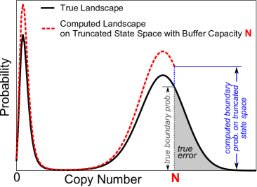
Figure 1: An illustration for the boundary probabilities. The solid black line represents the true probability landscape on the exact state space. The dashed red line represents the probability landscape computed from the truncated state space with buffer capacity $N$. The gray shaded area represents the true error due to state space truncation with buffer capacity $N$. The probability of copy number $N$ on the true landscape is the true boundary probability, and the probability of $N$ on the computed landscape is the boundary probability on the truncated state space. In this study, we show that the computed boundary probability on the truncated state space can be used to bound the true error from the above.

Figure 2: The birth-death system associated with the aggregated rate matrix $B$. Each circle represents an aggregated state consisting of all microstates with the same copy number of elementary molecules in the MEG. These aggregated states are connected by aggregated birth and death reactions, with apparent synthesis rates $\alpha_{i}$ and degradation rates $\beta_{i+1}$ (see Lemma 1).

Table 1: Reaction scheme and rate constants in phage lambda epigenetic switch mode. We use $CORn$ denotes $Cro_{2}$ bound operator site $ORn$, $RORn$ denotes $CI_{2}$ bound $ORn$, where $n$ can be 1, 2, and 3. Note that molecular species enclosed in parenthesis are those whose presence is required for the specific reactions to occur, but their copy numbers do not influence the transition rates between microstates.

Reactions	Rate constants
Synthesis reactions [50, 59, 60, 61]
$\emptyset+(OR3+OR2)\rightarrow CI_{2}+(OR3+OR2)$	$k_{sCI_{2}}=0.0069/s$
$\emptyset+(OR3+COR2)\rightarrow CI_{2}+(OR3+COR2)$	$k_{sCI_{2}}=0.0069/s$
$\emptyset+(OR3+ROR2)\rightarrow CI_{2}+(OR3+ROR2)$	$k_{s1CI_{2}}=0.069/s$
$\emptyset+(OR1+OR2)\rightarrow Cro_{2}+(OR1+OR2)$	$k_{sCro_{2}}=0.0929/s$
Degradation reactions [62, 50]
$CI_{2}\rightarrow\emptyset$	$k_{dCI_{2}}=0.0026/s$
$Cro_{2}\rightarrow\emptyset$	$k_{dCro_{2}}=0.0025/s$
Association rate of binding reactions [63]
$CI_{2}+OR1\rightarrow ROR1$	$k_{bOR1CI_{2}}=0.021/s$
$CI_{2}+OR2\rightarrow ROR2$	$k_{bOR2CI_{2}}=0.021/s$
$CI_{2}+OR3\rightarrow ROR3$	$k_{bOR3CI_{2}}=0.021/s$
$Cro_{2}+OR1\rightarrow COR1$	$k_{bOR1Cro_{2}}=0.021/s$
$Cro_{2}+OR2\rightarrow COR2$	$k_{bOR2Cro_{2}}=0.021/s$
$Cro_{2}+OR3\rightarrow COR3$	$k_{bOR3Cro_{2}}=0.021/s$
Dissociation reactions - $CI_{2}$ dissociation from OR1
$ROR1+(OR2)\rightarrow CI_{2}+OR1+(OR2)$	$0.00898/s$
$ROR1+(ROR2+OR3)\rightarrow CI_{2}+OR1+(ROR2+OR3)$	$0.00011/s$
$ROR1+(ROR2+ROR3)\rightarrow CI_{2}+OR1+(ROR2+ROR3)$	$0.01242/s$
$ROR1+(ROR2+COR3)\rightarrow CI_{2}+OR1+(ROR2+COR3)$	$0.00011/s$
$ROR1+(COR2)\rightarrow CI_{2}+OR1+(COR2)$	$0.00898/s$
Dissociation reactions - $CI_{2}$ dissociation from OR2
$ROR2+(OR1+OR3)\rightarrow CI_{2}+OR2+(OR1+OR3)$	$0.2297/s$
$ROR2+(ROR1+OR3)\rightarrow CI_{2}+OR2+(ROR1+OR3)$	$0.0029/s$
$ROR2+(OR1+ROR3)\rightarrow CI_{2}+OR2+(OR1+ROR3)$	$0.0021/s$
$ROR2+(ROR1+ROR3)\rightarrow CI_{2}+OR2+(ROR1+ROR3)$	$0.0029/s$
$ROR2+(COR1+OR3)\rightarrow CI_{2}+OR2+(COR1+OR3)$	$0.2297/s$
$ROR2+(OR1+COR3)\rightarrow CI_{2}+OR2+(OR1+COR3)$	$0.2297/s$
$ROR2+(COR1+COR3)\rightarrow CI_{2}+OR2+(COR1+COR3)$	$0.2297/s$
$ROR2+(ROR1+COR3)\rightarrow CI_{2}+OR2+(ROR1+COR3)$	$0.0029/s$
$ROR2+(COR1+ROR3)\rightarrow CI_{2}+OR2+(COR1+ROR3)$	$0.0021/s$
Dissociation reactions - CI dissociation from OR3
$ROR3+(OR2)\rightarrow CI_{2}+OR3+(OR2)$	$1.13/s$
$ROR3+(ROR2+OR1)\rightarrow CI_{2}+OR3+(ROR2+OR1)$	$0.0106/s$
$ROR3+(ROR2+ROR1)\rightarrow CI_{2}+OR3+(ROR2+ROR1)$	$0.0106/s$
$ROR3+(ROR2+COR1)\rightarrow CI_{2}+OR3+(ROR2+COR1)$	$0.0106/s$
$ROR3+(COR2)\rightarrow CI_{2}+OR3+(COR2)$	$1.13/s$
Dissociation reactions - Cro dissociation from OR1
$COR1+(OR2)\rightarrow Cro_{2}+OR1+(OR2)$	$0.0202/s$
$COR1+(ROR2)\rightarrow Cro_{2}+OR1+(ROR2)$	$0.0202/s$
$COR1+(COR2+OR3)\rightarrow Cro_{2}+OR1+(COR2+OR3)$	$0.0040/s$
$COR1+(COR2+ROR3)\rightarrow Cro_{2}+OR1+(COR2+ROR3)$	$0.0040/s$
$COR1+(COR2+COR3)\rightarrow Cro_{2}+OR1+(COR2+COR3)$	$0.0040/s$
Dissociation reactions - Cro dissociation from OR2
$COR2+(OR1+OR3)\rightarrow Cro_{2}+OR2+(OR1+OR3)$	$0.1413/s$
$COR2+(ROR1+OR3)\rightarrow Cro_{2}+OR2+(ROR1+OR3)$	$0.1413/s$
$COR2+(OR1+ROR3)\rightarrow Cro_{2}+OR2+(OR1+ROR3)$	$0.1413/s$
$COR2+(ROR1+ROR3)\rightarrow Cro_{2}+OR2+(ROR1+ROR3)$	$0.1413/s$
$COR2+(COR1+OR3)\rightarrow Cro_{2}+OR2+(COR1+OR3)$	$0.0279/s$
$COR2+(OR1+COR3)\rightarrow Cro_{2}+OR2+(OR1+COR3)$	$0.053/s$
$COR2+(COR1+COR3)\rightarrow Cro_{2}+OR2+(COR1+COR3)$	$0.0328/s$
$COR2+(ROR1+COR3)\rightarrow Cro_{2}+OR2+(ROR1+COR3)$	$0.053/s$
$COR2+(COR1+ROR3)\rightarrow Cro_{2}+OR2+(COR1+ROR3)$	$0.0279/s$
Dissociation reactions - Cro dissociation from OR3
$COR3+(OR2)\rightarrow Cro_{2}+OR3+(OR2)$	$0.0022/s$
$COR3+(ROR2)\rightarrow Cro_{2}+OR3+(ROR2)$	$0.0022/s$
$COR3+(COR2+OR1)\rightarrow Cro_{2}+OR3+(COR2+OR1)$	$0.0008/s$
$COR3+(COR2+ROR1)\rightarrow Cro_{2}+OR3+(COR2+ROR1)$	$0.0008/s$
$COR3+(COR2+COR1)\rightarrow Cro_{2}+OR3+(COR2+COR1)$	$0.003/s$

References

- 1. Jacob Stewart-Ornstein and Hana El-Samad. Stochastic modeling of cellular networks. Computational Methods in Cell Biology, 110:111, 2012.
- 2. Hong Qian. Cooperativity in cellular biochemical processes: noise-enhanced sensitivity, fluctuating enzyme, bistability with nonlinear feedback, and other mechanisms for sigmoidal responses. Annual Review of Biophysics, 41:179–204, 2012.
- 3. H.H. McAdams and A. Arkin. It’s a noisy business! Genetic regulation at the nanomolar scale. Trends in Genetics, 15(2):65–69, 1999.
- 4. Darren J Wilkinson. Stochastic modelling for quantitative description of heterogeneous biological systems. Nature Reviews Genetics, 10(2):122–133, 2009.
- 5. Youfang Cao, Hsiao-Mei Lu, and Jie Liang. Probability landscape of heritable and robust epigenetic state of lysogeny in phage lambda. Proceedings of the National Academy of Sciences of the United States of America, 107(43):18445–18450, 2010.
- 6. D. T. Gillespie. Exact stochastic simulation of coupled chemical reactions. Journal of Physical Chemistry, 81:2340–2361, 1977.
- 7. Daniel T. Gillespie. A rigorous derivation of the chemical master equation. Physica A, 188:404–425, 1992.
- 8. N.G. Van Kampen. Stochastic processes in physics and chemistry, 3rd Edition. Elsevier Science and Technology books, 2007.
- 9. D.A. Beard and H. Qian. Chemical biophysics: quantitative analysis of cellular systems. Cambridge Univ Pr, 2008.
- 10. Daniel T. Gillespie. A diffusional bimolecular propensity function. The Journal of Chemical Physics, 131(16):164109, 2009.
- 11. I.G. Darvey, B.W. Ninham, and P.J. Staff. Stochastic models for second order chemical reaction kinetics. the equilibrium state. The Journal of Chemical Physics, 45:2145–2155, 1966.
- 12. D.A. McQuarrie. Stochastic approach to chemical kinetics. Journal of Applied Probability, 4:413–478, 1967.
- 13. H.M. Taylor and S. Karlin. An Introduction to Stochastic Modeling, 3rd Ed. Academic Press, 1998.
- 14. I.J. Laurenzi. An analytical solution of the stochastic master equation for reversible bimolecular reaction kinetics. The Journal of Chemical Physics, 113:3315–3322, 2000.
- 15. Melissa Vellela and Hong Qian. A quasistationary analysis of a stochastic chemical reaction: Keizer’s paradox. Bulletin of Mathematical Biology, 69(5):1727–1746, 2007.
- 16. Daniel. T. Gillespie. The chemical langevin equation. The Journal of Chemical Physics, 113:297–306, 2000.
- 17. N. G. Van Kampen. A power series expansion of the master equation. Canadian Journal of Physics, 39(4):551–567, 1961.
- 18. Daniel T. Gillespie. The chemical Langevin and Fokker−Planck equations for the reversible isomerization reaction†. The Journal of Physical Chemistry A, 106(20):5063–5071, 2002.
- 19. Eric L. Haseltine and James B. Rawlings. Approximate simulation of coupled fast and slow reactions for stochastic chemical kinetics. The Journal of Chemical Physics, 117(15):6959–6969, 2002.
- 20. C. W. Gardiner. Handbook of Stochastic Methods for Physics, Chemistry and the Natural Sciences. Springer, New York, 2004.
- 21. R. Grima, P. Thomas, and A. V. Straube. How accurate are the nonlinear chemical Fokker-Planck and chemical Langevin equations? The Journal of Chemical Physics, 135(8):084103, Aug 2011.
- 22. P. Thomas, H. Matuschek, and R. Grima. How reliable is the linear noise approximation of gene regulatory networks? BMC Genomics, 14 Suppl 4:S5, 2013.
- 23. Brian Munsky and Mustafa Khammash. The finite state projection algorithm for the solution of the chemical master equation. The Journal of Chemical Physics, 124(4):044104, 2006.
- 24. Youfang Cao and Jie Liang. Optimal enumeration of state space of finitely buffered stochastic molecular networks and exact computation of steady state landscape probability. BMC Systems Biology, 2(1):30, 2008.
- 25. Shev MacNamara, Alberto M Bersani, Kevin Burrage, and Roger B Sidje. Stochastic chemical kinetics and the total quasi-steady-state assumption: application to the stochastic simulation algorithm and chemical master equation. The Journal of chemical physics, 129(9):095105, 2008.
- 26. Shev MacNamara, Kevin Burrage, and Roger B Sidje. Multiscale modeling of chemical kinetics via the master equation. Multiscale Modeling & Simulation, 6(4):1146–1168, 2008.
- 27. Verena Wolf, Rushil Goel, Maria Mateescu, and Thomas Henzinger. Solving the chemical master equation using sliding windows. BMC Systems Biology, 4(1):42, 2010.
- 28. Tobias Jahnke. On reduced models for the chemical master equation. Multiscale Modeling & Simulation, 9(4):1646–1676, 2011.
- 29. Roger B Sidje. Expokit: a software package for computing matrix exponentials. ACM Transactions on Mathematical Software (TOMS), 24(1):130–156, 1998.
- 30. Brian Munsky and Mustafa Khammash. A multiple time interval finite state projection algorithm for the solution to the chemical master equation. Journal of Computational Physics, 226(1):818 – 835, 2007.
- 31. Jianjun Paul Tian and D Kannan. Lumpability and commutativity of Markov processes. Stochastic analysis and Applications, 24(3):685–702, 2006.
- 32. Laurent Truffet. Near complete decomposability: bounding the error by a stochastic comparison method. Advances in Applied Probability, pages 830–855, 1997.
- 33. Peter Buchholz. Exact and ordinary lumpability in finite Markov chains. Journal of Applied Probability, pages 59–75, 1994.
- 34. W.J. Stewart. Introduction to the numerical solution of Markov chains. Princeton University Press NJ, 1994.
- 35. Hendrik Vantilborgh. Aggregation with an error of o. Journal of the ACM (JACM), 32(1):162–190, 1985.
- 36. John G Kemeny and James Laurie Snell. Finite Markov chains, volume 210. Springer-Verlag New York, 1976.
- 37. A Irle. Stochastic ordering for continuous-time processes. Journal of Applied Probability, pages 361–375, 2003.
- 38. B.J. Daigle, M.K. Roh, D.T. Gillespie, and L.R. Petzold. Automated estimation of rare event probabilities in biochemical systems. The Journal of Chemical Physics, 134:044110, 2011.
- 39. M.K. Roh, B.J. Daigle, D.T. Gillespie, and L.R. Petzold. State-dependent doubly weighted stochastic simulation algorithm for automatic characterization of stochastic biochemical rare events. Journal of Chemical Physics, 135(23):234108, 2011.
- 40. Youfang Cao and Jie Liang. Adaptively biased sequential importance sampling for rare events in reaction networks with comparison to exact solutions from finite buffer dCME method. The Journal of Chemical Physics, 139(2):025101, 2013.
- 41. Yuichi Taniguchi, Paul J Choi, Gene-Wei Li, Huiyi Chen, Mohan Babu, Jeremy Hearn, Andrew Emili, and X Sunney Xie. Quantifying e. coli proteome and transcriptome with single-molecule sensitivity in single cells. Science, 329(5991):533–538, 2010.
- 42. Timothy S Gardner, Charles R Cantor, and James J Collins. Construction of a genetic toggle switch in Escherichia coli. Nature, 403(6767):339–342, 2000.
- 43. Thomas B Kepler and Timothy C Elston. Stochasticity in transcriptional regulation: origins, consequences, and mathematical representations. Biophysical Journal, 81(6):3116–3136, 2001.
- 44. Keun-Young Kim and Jin Wang. Potential energy landscape and robustness of a gene regulatory network: toggle switch. PLoS Computational Biology, 3(3):e60, 2007.
- 45. D. Schultz, J. N. Onuchic, and P. G. Wolynes. Understanding stochastic simulations of the smallest genetic networks. The Journal of Chemical Physics, 126(24):245102, 2007.
- 46. Brian Munsky and Mustafa Khammash. The finite state projection approach for the analysis of stochastic noise in gene networks. Automatic Control, IEEE Transactions on, 53(Special Issue):201–214, 2008.
- 47. Peter Deuflhard, Wilhelm Huisinga, T Jahnke, and Michael Wulkow. Adaptive discrete Galerkin methods applied to the chemical master equation. SIAM Journal on Scientific Computing, 30(6):2990–3011, 2008.
- 48. Paul Sjöberg, Per Lötstedt, and Johan Elf. Fokker–Planck approximation of the master equation in molecular biology. Computing and Visualization in Science, 12(1):37–50, 2009.
- 49. Vladimir Kazeev, Mustafa Khammash, Michael Nip, and Christoph Schwab. Direct solution of the chemical master equation using quantized tensor trains. PLoS Computational Biology, 10(3):e1003359, 03 2014.
- 50. Adam Arkin, John Ross, and Harley H. McAdams. Stochastic kinetic analysis of developmental pathway bifurcation in phage -infected Escherichia coli cells. Genetics, 149(4):1633–1648, 1998.
- 51. Erik Aurell, Stanley Brown, Johan Johanson, and Kim Sneppen. Stability puzzles in phage . Physical Review E, 65(5):051914, 2002.
- 52. Erik Aurell and Kim Sneppen. Epigenetics as a first exit problem. Physical Review Letters, 88(4):048101, 2002.
- 53. X.-M. Zhu, L. Yin, L. Hood, and P. Ao. Robustness, stability and efficiency of phage lambda genetic switch: dynamical structure analysis. Journal of Bioinformatics and Computational Biology, 2:785–817, 2004.
- 54. X.-M. Zhu, L. Yin, L. Hood, and P. Ao. Calculating biological behaviors of epigenetic states in the phage life cycle. Functional & Integrative Genomics, 4(3):188–195, 2004.
- 55. Shuohao Liao, T Vejchodsky, and Radek Erban. Tensor methods for parameter estimation and bifurcation analysis of stochastic reaction networks. Journal of the Royal Society Interface, 12(108):20150233, 2015.
- 56. F. Verstraete and J. I. Cirac. Matrix product states represent ground states faithfully. Phys. Rev. B, 73:094423, Mar 2006.
- 57. Philip Nelson. Physical Models of Living Systems. Macmillan, 2015.
- 58. Carl D Meyer. Matrix analysis and applied linear algebra. SIAM, 2000.
- 59. M. Li, W. McClure, and M. Susskind. Changing the mechanism of transcriptional activation by phage lambda repressor. Proceedings of the National Academy of Sciences of the United States of America, 94(8):3691–3696, 1997.
- 60. D. Hawley and W. McClure. In vitro comparison of initiation properties of bacteriophage lambda wild-type PR and x3 mutant promoters. Proceedings of the National Academy of Sciences of the United States of America, 77(11):6381–6385, 1980.
- 61. D. Hawley and W. McClure. Mechanism of activation of transcription initiation from the lambda PRM promoter. Journal of Molecular Biology, 157(3):493–525, 1982.
- 62. Madeline A. Shea and Gary K. Ackers. The control system of bacteriophage lambda a physical-chemical model for gene regulation. Journal of Molecular Biology, 181(2):211–230, 1985.
- 63. Céline Kuttler and Joachim Niehren. Gene Regulation in the Pi Calculus: Simulating Cooperativity at the Lambda Switch. Transactions on Computational Systems Biology VII, 4230:24–55, 2006.