Probabilistic Graphical Models for
Credibility Analysis in
Evolving Online Communities

Subhabrata Mukherjee
Max-Planck-Institut für Informatik

Dissertation
zur Erlangung des Grades
des Doktors der Ingenieurwissenschaften (Dr.-Ing.)
der Fakultät für Mathematik und Informatik
der Universität des Saarlandes

Saarbrücken
March 2017

Dean	Prof. Dr. Frank-Olaf Schreyer
	Faculty of Mathematics and Computer Sciences
	Saarland University
	Saarbrücken, Germany
Colloquium	July 6, 2017
	Saarbrücken, Germany
Examination	Board
Advisor and	Prof. Dr. Gerhard Weikum
First Reviewer	Department of Databases and Information Systems
	Max Planck Institute for Informatics
	Saarbrücken, Germany
Second Reviewer	Prof. Dr. Jiawei Han
	Department of Computer Science
	University of Illinois at Urbana-Champaign
	Urbana, USA
Third Reviewer	Prof. Dr. Stephan Günnemann
	Department of Informatics
	Technical University of Munich
	Munich, Germany
Chairman	Prof. Dr. Dietrich Klakow
	Department of Computer Science
	Saarland University
	Saarbrücken, Germany
Research	Dr. Rishiraj Saha Roy
Assistant	Department of Databases and Information Systems
	Max Planck Institute for Informatics
	Saarbrücken, Germany

“Note to self: every time you were convinced you couldn’t go on,
you did.”
— Unknown

Abstract

One of the major hurdles preventing the full exploitation of information from online communities is the widespread concern regarding the quality and credibility of user-contributed content. Prior works in this domain operate on a static snapshot of the community, making strong assumptions about the structure of the data (e.g., relational tables), or consider only shallow features for text classification.

To address the above limitations, we propose probabilistic graphical models that can leverage the joint interplay between multiple factors in online communities — like user interactions, community dynamics, and textual content — to automatically assess the credibility of user-contributed online content, and the expertise of users and their evolution with user-interpretable explanation. To this end, we devise new models based on Conditional Random Fields for different settings like incorporating partial expert knowledge for semi-supervised learning, and handling discrete labels as well as numeric ratings for fine-grained analysis. This enables applications such as extracting reliable side-effects of drugs from user-contributed posts in healthforums, and identifying credible content in news communities.

Online communities are dynamic, as users join and leave, adapt to evolving trends, and mature over time. To capture this dynamics, we propose generative models based on Hidden Markov Model, Latent Dirichlet Allocation, and Brownian Motion to trace the continuous evolution of user expertise and their language model over time. This allows us to identify expert users and credible content jointly over time, improving state-of-the-art recommender systems by explicitly considering the maturity of users. This also enables applications such as identifying helpful product reviews, and detecting fake and anomalous reviews with limited information.

Kurzfassung

Eine der größten Hürden, die die vollständige Nutzung von Informationen aus sogenannten Online-Communities verhindert, sind weitverbreitete Bedenken bezüglich der Qualität und Glaubwürdigkeit von Nutzer-generierten Inhalten. Frühere Arbeiten in diesem Bereich gehen von einer statischen Version einer Community aus, machen starke Annahmen bezüglich der Struktur der Daten (z.B. relationale Tabellen) oder berücksichtigen nur oberflächliche Merkmale zur Klassifikation von Texten.

Um die oben genannten Einschränkungen zu adressieren, schlagen wir eine Reihe von probabilistischen graphischen Modellen vor, die das Zusammenspiel mehrerer Faktoren in Online-Communities berücksichtigen: Interaktionen zwischen Nutzern, die Dynamik in Communities und der textuell Inhalt. Dadurch können die Glaubwürdigkeit von Nutzer-generierten Online Inhalten sowie die Expertise von Nutzern und ihrer Entwicklung mit interpretierbaren Erklärungen bewertet werden. Hierfür konstruieren wir neue, auf Conditional Random Fields basierende Modelle für verschiedene Szenarien, um beispielsweise partielles Expertenwissen mittels semi-überwachtem Lernen zu berücksichtigen. Genauso können diskrete Labels sowie numerische Ratings für präzise Analysen genutzt werden. Somit werden Anwendungen ermöglicht wie etwa das automatische Extrahieren von Nebenwirkungen von Medikamenten aus Nutzer-erstellten Inhalten in Gesundheitsforen und das Identifizieren von vertrauenswürdigen Inhalten aus Nachrichten-Communities.

Online-Communities sind dynamisch, da Nutzer zu Communities hinzustoßen oder diese verlassen. Sie passen sich entstehenden Trends an und entwickeln sich über die Zeit. Um diese Dynamik abzudecken, schlagen wir generative Modelle vor, die auf Hidden Markov Modellen, Latent Dirichlet Allocation und Brownian Motion basieren. Diese können die kontinuierliche Entwicklung von Nutzer-Erfahrung sowie ihrer Sprachentwicklung über die Zeit nachzeichnen. Dies ermöglicht uns, Expertennutzer und glaubwürdigen Inhalt über die Zeit gemeinsam zu identifizieren, sodass die aktuell besten Recommender- Systeme durch das explizite Berücksichtigen der Entwicklung und der Expertise von Nutzern verbessert werden können. Dadurch wiederum können Anwendungen entwickelt werden, die nützliche Produktbewertungen erkennen sowie fingierte und anomale Bewertungen mit geringem Informationsgehalt identifizieren.

Contents

1. Acknowledgements
2. Abstract
3. Kurzfassung
4. I Introduction
   1. I.1 Motivation
   2. I.2 Challenges
   3. I.3 Prior Work and its Limitations
   4. I.4 Contributions
   5. I.5 Organization
5. II Related Work
   1. II.1 Probabilistic Graphical Models
   2. II.2 Truth Discovery
   3. II.3 Trust and Reputation Management
   4. II.4 Information Extraction (IE)
   5. II.5 Language Analysis for Social Media
   6. II.6 Information Credibility in Social Media
   7. II.7 Collaborative Filtering for Online Communities
6. III Credibility Analysis Framework
   1. III.1 Introduction and Motivation
      1. III.1.1 Use-case Study: Health Communities
      2. III.1.2 Use-case Study: News Communities
      3. III.1.3 Contributions
   2. III.2 Problem Statement
   3. III.3 Overview of the Model
      1. III.3.1 Credibility Classification
      2. III.3.2 Credibility Regression
   4. III.4 Model Components
      1. III.4.1 Postings and their Language
         1. Stylistic
         2. Affective
         3. Bias and Subjectivity
      2. III.4.2 User Expertise
      3. III.4.3 Postings and their Topics
      4. III.4.4 Sources
   5. III.5 Probabilistic Inference
      1. III.5.1 Semi-supervised Conditional Random Fields for Credibility Classification
      2. III.5.2 Continuous Conditional Random Fields for Credibility Regression
         1. Topic Model
         2. Support Vector Regression
         3. Continuous Conditional Random Field
   6. III.6 Experimental Evaluation: Health Communities
      1. III.6.1 Data
      2. III.6.2 Baselines
      3. III.6.3 Experiments and Quality Measures
      4. III.6.4 Results and Discussions
      5. III.6.5 Discovering Rare Side Effects
      6. III.6.6 Following Trustworthy Users
   7. III.7 Experimental Evaluation: News Communities
      1. III.7.1 Data
      2. III.7.2 Predicting User Credibility Ratings of News Articles
      3. III.7.3 Finding Credible News Articles
      4. III.7.4 Finding Trustworthy Sources
      5. III.7.5 Finding Expert Users
      6. III.7.6 Discussion
   8. III.8 Conclusions
7. IV Temporal Evolution of Online Communities
   1. IV.1 Introduction
   2. IV.2 Motivation and Approach
      1. IV.2.1 Discete Experience Evolution
      2. IV.2.2 Continuous Experience Evolution
   3. IV.3 Discrete Experience Evolution
      1. IV.3.1 Model Dimensions
      2. IV.3.2 Hypotheses and Initial Studies
      3. IV.3.3 Building Blocks of our Model
         1. Latent Factor Recommendation
         2. Experience-based Latent Factor Recommendation
         3. User-Facet Model
         4. Supervised User-Facet Model
      4. IV.3.4 Joint Model: User Experience, Facet Preference, Writing Style
         1. Generative Process for a Review
         2. Supervision for Rating Prediction
         3. Inference
      5. IV.3.5 Experiments
         1. Setup: Data and Baselines
         2. Quantitative Comparison
         3. Qualitative Analysis
   4. IV.4 Continuous Experience Evolution
      1. IV.4.1 Model Components
         1. Importance of Time
         2. Continuous Experience Evolution
         3. Experience-aware Language Evolution
      2. IV.4.2 Joint Model for Experience-Language Evolution
         1. Generative Process
         2. Inference
      3. IV.4.3 Experiments
         1. Data Likelihood, Smoothness and Convergence
         2. Experience-aware Item Rating Prediction
         3. Quantitative Results
         4. Qualitative Results
   5. IV.5 Use-Case Study
      1. IV.5.1 Recommending News Articles
      2. IV.5.2 Identifying Experienced Users
   6. IV.6 Conclusion
8. V Credibility Analysis of Product Reviews
   1. V.1 Introduction
   2. V.2 Motivation and Approach
      1. V.2.1 Finding Useful Product Reviews
      2. V.2.2 Finding Credible Reviews with Limited Information
   3. V.3 Exploring Latent Semantic Factors to Find Useful Product Reviews
      1. V.3.1 Review Helpfulness Factors
         1. Item Facets
         2. Review Writing Style
         3. Reviewer Expertise
         4. Distributional Hypotheses
         5. Consistency
         6. Timeliness or “Early-bird” bias
         7. Preliminary Study of Feature Significance
      2. V.3.2 Joint Model for Review Helpfulness
         1. Incorporating Consistency Factors
         2. Incorporating Latent Facets
         3. Incorporating Latent Expertise
         4. Difference with Prior Works for Modeling Expertise
         5. Generative Process
         6. Inference
      3. V.3.3 Experiments
         1. Setup: Data
         2. Tasks and Evaluation Measures
         3. Baselines
         4. Quantitative Comparison
         5. Qualitative Comparison
   4. V.4 Finding Credible Reviews with Limited Information using Consistency Features
      1. V.4.1 Review Credibility Analysis
         1. Facet Model
         2. Consistency Features
         3. Additional Language and Behavioral Features
      2. V.4.2 Tasks
         1. Credible Review Classification
         2. Item Ranking and Evaluation Measures
         3. Domain Transfer from Yelp to Amazon
         4. Ranking SVM
      3. V.4.3 Experiments
         1. Setup and Data
         2. Baselines
         3. Quantitative Analysis
         4. Qualitative Analysis
   5. V.5 Conclusions
9. VI Conclusions
   1. VI.1 Contributions
   2. VI.2 Outlook
10. References

List of Figures

1. III.1 Overview of the proposed model, which captures the interactions between statement credibility, posting objectivity, and user trustworthiness.
2. III.2 Graphical model representation.
3. (a) Interactions between source trustworthiness, posting (i.e. article) credibility, language objectivity, and user expertise.
4. (b) Sample instantiation.
5. (c) Clique representation.
6. III.3 Specificity and sensitivity comparison of models.
7. IV.1 $KL$ Divergence as a function of experience.
8. (a) Divergence of language model as a function of experience.
9. (b) Divergence of facet preference as a function of experience.
10. IV.2 Supervised model for user facets and ratings.
11. IV.3 Supervised model for user experience, facets, and ratings.
12. IV.4 MSE improvement (%) of our model over baselines.
13. IV.5 Proportion of reviews at each experience level of users.
14. IV.6 Facet preference and language model $KL$ divergence with experience.
15. (a) User at learned rate [McAuley 2013b]: Facet preference divergence with experience.
16. (b) Our model: Facet preference divergence with experience.
17. (c) Our model: Language model divergence with experience.
18. IV.7 Discrete state and continuous state experience evolution of some typical users from the BeerAdvocate community.
19. (a) Evolution of an experienced user.
20. (b) Evolution of an amateur user.
21. IV.8 Continuous experience-aware language model. Words (shaded in blue), and timestamps (not shown for brevity) are observed.
22. IV.9 Log-likelihood per iteration of discrete model (refer to Section IV.3) vs. continuous experience model (this work).
23. IV.10  Variation of experience ($e$) with years and reviews of each user. Each bar in the above stacked chart corresponds to a user with her most recent experience, number of years spent, and number of reviews posted in the community.
24. IV.11  Variation of experience ($e$) with mean ($\mu_{u}$) and variance ($\sigma_{u}$) of the GBM trajectory of each user ($u$). Each bar in the above stacked chart corresponds to a user with her most recent experience, mean and variance of her experience evolution.
25. IV.12  Variation of word frequency with word experience. Each point in the above scatter plot corresponds to a word ($w$) in “2011” with corresponding frequency and experience value ($l_{t\text{=2011},w}$).
26. IV.13  Language model score ($\beta_{t,z,w}\boldsymbol{\cdot}l_{t,w}$) variation for sample words with time. Figure a) shows the count of some sample words over time in BeerAdvocate community, whose evolution is traced in Figure b). Figures c) and d) show the evolution in Yelp and Amazon Movies.
27. V.1 Generative process for helpful product reviews.
28. V.2 Increase in log-likelihood (scaled by $10e+07$) of the data per-iteration in the five domains.
29. V.3 Facet preference and language model KL divergence with expertise.
30. (a) Our model: Facet preference divergence with expertise learned from review helpfulness.
31. (b) Our model: Language model divergence with expertise learned from review helpfulness.
32. V.4 Variation of Kendall-Tau-M ($\tau_{m}$) on different Amazon domains with parameter $C^{-}$ variation (using model $M_{\text{Yelp}}$ trained in Yelp and tested in Amazon).

List of Tables

1. III.1 Stylistic features.
2. III.2 Examples of affective features.
3. III.3 Subjectivity and bias features.
4. III.4 Latent topics (with illustrative labels) and their words.
5. III.5 Features for source trustworthiness.
6. III.6 Symbol table.
7. III.7 User statistics.
8. III.8 Information on sample drug families: number of postings and number of users reporting at least one side effect.
9. III.9 Number of common, less common, and rare side-effects listed by experts on Mayo Clinic.
10. III.10  Accuracy comparison in setting I.
11. III.11  CRF performance in setting II.
12. III.12  Experiment on finding rare drug side-effects.
13. III.13  Experiment on following trustworthy users.
14. III.14  Dataset statistics.
15. III.15  Graph statistics.
16. III.16  MSE comparison of models for predicting users’ credibility rating behavior with $10$-fold cross-validation. Improvements are statistically significant with P-value < $0.0001$.
17. III.17  MSE comparison of models for predicting aggregated article credibility rating with $10$-fold cross-validation. Improvements are statistically significant with P-value < $0.0001$.
18. III.7.3 Finding Credible News Articles
19. III.20  Pearson’s product-moment correlation between various factors (with P-value $<0.0001$ for each test).
20. III.21  Most and least trusted sources on sample topics.
21. III.22  Most and least trusted sources with different viewpoints.
22. III.23  Most and least trusted sources on different types of media.
23. IV.1 Vocabulary at different experience levels.
24. IV.2 Salient words for two facets at five experience levels in movie reviews.
25. IV.3 Dataset statistics.
26. IV.4 MSE comparison of our model versus baselines.
27. IV.5 Experience-based facet words for the illustrative beer facet taste.
28. IV.6 Distribution of users at different experience levels.
29. IV.7 Dataset statistics.
30. IV.8 Mean squared error (MSE) for rating prediction. Our model performs better than competing methods.
31. IV.9  Top words used by experienced and amateur users.
32. IV.10  Salient words for the illustrative NewsTrust topic US Election used by users at different levels of experience.
33. IV.11  Performance on identifying experienced users.
34. V.1 Pearson correlation between different features and helpfulness scores of reviews in the domains electronics, foods, music, movies, and books. All factors (except the one marked with $*$) are statistically significant with p-value $<2e-16$.
35. V.2 Dataset statistics. Votes indicate the total number of helpfulness votes (both, for and against) cast for a review. Total number of users $=5,679,944$, items $=1,895,462$, and reviews $=29,004,754$.
36. V.3 Prediction Task: Performance comparison of our model versus baselines. Our improvements over the baselines are statistically significant at p-value $<2.2e-16$ using paired sample t-test.
37. V.4 Ranking Task: Correlation comparison between the ranking of reviews and gold rank list — our model versus baselines. Our improvements over the baselines are statistically significant at p-value $<2.2e-16$ using paired sample t-test.
38. V.5 Snapshot of latent word clusters as used by experts and amateurs for most and least helpful reviews in different domains.
39. V.6 List of variables and notations used with corresponding description.
40. V.7 Dataset statistics for review classification (Yelp^∗ denotes balanced dataset using random sampling).
41. V.8 Amazon dataset statistics for item ranking, with cumulative #items and varying #reviews.
42. V.9 Credible review classification accuracy with $10$-fold cross validation. TripAdvisor dataset contains only review texts and no user/activity information.
43. V.10   Kendall-Tau correlation of different models across domains.
44. V.11   Variation of Kendall-Tau-M ($\tau_{m}$) correlation with #reviews with $M_{\text{Amazon}}$ (SVM-Rank).
45. V.12   Top n-grams (by feature weights) for credibility classification.
46. V.13   Snapshot of non-credible reviews (reproduced verbatim) with inconsistencies.

Introduction

I.1 Motivation

In recent years, the explosion of social networking sites (e.g., Facebook, Twitter), blogs (e.g., Mashable, Techcrunch), and online review portals (e.g., Amazon, TripAdvisor, IMDB, Healthboards) provide overwhelming amount of information on various topics like health, politics, movies, music, travel, and more. However, the usability of such massive data is largely restricted due to concerns about the quality and credibility of user-contributed content.

Online communities are massive repositories of knowledge that are accessed by regular everyday users as well as expert professionals. For instance, $59\%$ of the adult U.S. population and nearly half of U.S. physicians consult online resources (e.g., Youtube and Wikipedia) [Fox 2013, IMS Institute 2014] for health-related information. In the product domain, $40\%$ of online consumers would not buy electronics without consulting online reviews first [Nielsen]. However, this user-contributed content is highly noisy, unreliable, and subjective with rampant amount of spams, rumors, and misinformation injected by users in their postings. This has greatly eroded public trust and confidence on social media information. Some statistics show that $66\%$ of web-using U.S. adults do not trust social media information [Mitchell 2016]. To counter these, stakeholders in the industry (e.g., Yelp) have been developing their own defense mechanism. In certain domains like healthforums, misinformation can have hazardous consequences — as these are frequently accessed by users to find potential side-effects of drugs, symptoms of diseases, or getting advice from health professionals. To give an example, consider the following user-post from the online healthforum Healthboards.

Example I.1.1

I took a cocktail of meds. Xanax gave me hallucinations and a demonic feel. I can feel my skin peeling off.

The above post suggests that “peeling-of-skin” is a probable side-effect of the drug Xanax, although the style in which it is written renders its credibility doubtful.

In this case, the user seems to be suffering from hallucinations; and the side-effect can also be attributed to the “cocktail of meds”, and not Xanax alone.

Prior works in Natural Language Processing dealing with fake reviews and opinion spam [Mihalcea 2009, Ott 2011, Recasens 2013, Li 2014b] would only analyze the linguistic cues and writing style of this post (e.g., distribution of unigrams and bigrams, affective emotions, part-of-speech tags, etc.) to find if it is subjective, biased, or fake. However, it is difficult to arrive at a conclusion by analyzing the post in isolation. In general, online communities provide many other signals that can help us in this task. For instance, the above post may be refuted (or downvoted) by an experienced health professional in the community. Similarly, credible postings or statements may be corroborated (or upvoted) by other experienced users in the community. A significant challenge is that a priori we do not know which users are experienced or trustworthy — that need to be inferred as a part of the task. These kinds of implicit or explicit feedback from other users, and their identities, prove to be helpful for credibility analysis in a community-specific setting.

Prior works in Data Fusion and Truth Discovery (cf. [Li 2015b] for a survey) leverage such interactions between sources and queries in a general setting. Some typical queries are “the height of Mount Everest” that fetch different answers (e.g., “29,035 feet”, “29,002 feet”, “29,029 feet”) from various sources, or “the birthplace of Obama” that includes answers as “Hawaii”, “USA”, and “Africa”. These methods aim to resolve conflicts among these multi-source data by obtaining reliability estimates of the sources providing the information (e.g., Wikipedia being a trustworthy source provides an accurate answer to the above queries), and aggregating their responses to obtain the truth. However, these approaches operate over structured data (e.g., relational tables, structured query templates like “Obama_BornIn_Kenya” represented as a subject-predicate-object triple), and factual claims — whereby they ignore the content and context of information. These approaches are not geared for online communities with more fine-grained interactions, subjective, and unstructured data. Context helps us in understanding the attitude and emotional state of the user writing the posts, the topics of the postings and users’ topic-specific expertise, objectivity and rationality of the postings, etc. Similar principles hold true for any online community like music, travel, politics, and news.

The above discussion demonstrates the complex interplay between several factors in online communities — like writing style, cross-talk between users and interactions, user experience, and topics — that influences the credibility of statements therein. A natural way to represent these interactions and dependencies between various factors is provided by Probabilistic Graphical Models (PGM) (like, Markov Random Fields, Bayesian Networks, and Factor Graphs) [Koller 2009], where each of the above aspects can be envisioned as random variables with edges depicting interactions between them.

PGMs provide a natural framework to compactly represent high-dimensional distributions over many random variables as a product of local factors over subsets of the variables, i.e., by factoring the joint probability distribution into marginal distributions over subsets of the variables. The conditional independence assumptions, and factorization help us to make the problem tractable. It is also effective in practice as any random variable interacts with only a subset of all the variables. During inference and learning, we estimate the joint probability distribution, the marginals, and other queries of interest. In terms of interpretability, output of probabilistic models (labels, probabilities of queries and factors) can be better explained to the end-user. For instance, a PGM may label two sources as “trustworthy” with corresponding probabilities as $0.9$ and $0.7$ — which is easier to envision than obtaining corresponding raw estimates as $12.7$ and $9.6$.

The key contribution of this work is in bringing all of these different aspects together in a computational model, namely, a probabilistic graphical model, for credibility analysis in online communities, and providing efficient inference techniques for the same.

I.2 Challenges

Analyzing the credibility of user-contributed content in online communities is a difficult task with the following challenges:

• User-contributed postings in online forums are unstructured, biased, and subjective in nature. This is in contrast to the classical setting in prior works in Truth Discovery and Data Fusion that deal with structured and factual data.

• Although reliable sources and users contribute credible information, a priori we do not know which of these sources and users are trustworthy (or experts).

• Online communities are complex in nature with rich user-user and user-item interactions (like, upvote, downvote, share, comment, etc.) that are difficult to model computationally.

• Online communities are dynamic in nature as users’ interactions, maturity, and content evolve over time.

• Scarcity of labeled training data and rich statistics (e.g., activity history, meta-data) about users and items lead to data sparsity and difficulty in learning.

• It is difficult to generate user-interpretable explanations of the models’ verdict.

I.3 Prior Work and its Limitations

Information extraction methods [Sarawagi 2008, Koller 2009] previously used for extracting information from user-contributed content do not account for the inherent bias, subjectivity, and noise in the data. Additionally, they also do not consider the role of language (e.g., stylistic features, emotional state and attitude of the writer, etc.) in assessing the reliability of the extracted statements.

Prior works in Natural Language Processing [Mihalcea 2009, Ott 2011, Recasens 2013, Li 2014b], dealing with opinion spam and fake reviews in online communities, consider postings in isolation, and analyze their writing style to capture bias and subjectivity. They typically ignore the identity of the users writing the postings, and interactions between them. Typically these works use bag-of-words features, and resources like WordNet [Miller 1995], and SentiWordNet [Esuli 2006] to create feature vectors that are fed into supervised machine learning models (e.g., Support Vector Machines) to classify the postings as credible, or otherwise.

On the other hand, works in Data Fusion and Truth Discovery (cf. [Li 2015b] for a survey) make strong assumptions about the nature and structure of the data (e.g., relational tables, factual claims, static data, subject-predicate-object triples, etc.) whereby they model the interactions between sources and queries as edges in a network, but ignore the textual content and context altogether. Typically, these works use approaches like belief propagation and label propagation (e.g., Markov random walks) to propagate reliability estimates in the network. Availability of ground-truth data is a typical problem faced by the works in this domain. Therefore, most of these prior works operate in an unsupervised fashion. However, some prior works show that the performance of these methods can be improved by using a small set of labeled data for training.

In the absence of proper ground-truth data, prior works [Jindal 2007, Jindal 2008, Lim 2010, Liu 2012, Mukherjee 2013a, Li 2014a, Rahman 2015] make strong assumptions, e.g., duplicates and near-duplicates are fake, and harness rich information about users and items in the form of activity, posting history, and meta-data. Such profile history may not be readily available in several domains, especially for “long-tail” users and items in the community (e.g., newcomers and recently launched products). Also, such a policy tends to over emphasize long-term contributors and suppress outlier opinions off the mainstream.

Prior works in collaborative filtering [Koren 2008, Koren 2015, Jindal 2008, Tang 2013, Ma 2015] consider a static snapshot of the data whereby they ignore the temporal evolution of users and their interactions. These use activity history (e.g., frequency of postings, number of upvotes / downvotes, rating history) as a proxy to find experienced members in the community. Online communities are dynamic in nature as users join and leave, adopt new vocabulary, and adapt to evolving trends. Therefore, a user who was not experienced a decade before could have evolved into a matured user now with refined preferences, writing style, and trustworthiness. This dimension of user evolution is ignored in the static analysis.

Most of the works involving classifiers and machine learning models generate discrete (e.g., binary) decision labels as output. These models have limited interpretability as they rarely explain why the model arrived at a particular verdict. Most of these are not geared for fine-grained analysis involving continuous data types. Additionally, most of the prior works output only raw scores, as estimates of reliability, that are difficult to explain to the end-user.

I.4 Contributions

This work addresses the challenges outlined above developing principles and models to advance the state-of-the-art. In summary, it addresses the following research questions.

RQ: 1

How can we develop models that jointly leverage the context and interactions in online communities for analyzing the credibility of user-contributed content? How can we complement expert knowledge with large-scale non-expert data from online communities?

We develop novel forms of probabilistic graphical models that capture the complex interplay between several factors: the writing style, user-user and user-item interactions, latent semantic factors like the topics of the postings and experience of the users, etc. Specifically, we develop Conditional Random Field (CRF) based models, where these factors (e.g., users, postings, statements) are modeled as random variables with edges between them depicting interactions. Furthermore, these variables have observable features that capture the context (e.g., stylistic features, subjectivity, topics, etc.) of the postings and relevant background information (e.g., user demographics and activity history). We develop efficient joint probabilistic inference techniques for these models for classification and regression settings. Specifically, we develop:

• A semi-supervised version of the CRF for credibility classification (presented at SIGKDD 2014 [Mukherjee 2014b]) that learns from partial expert supervision using Expectation - Maximization principle. We use this model in a healthforum Healthboards to identify rare or uncommon side-effects of drugs from user-contributed posts. This is one of the problems where large-scale non-expert data has the potential to complement expert medical knowledge. Our model leverages partial expert knowledge of drugs and their side-effects to jointly identify credible statements (or, drug side-effects), reliable postings, and trustworthy users in the community.

• A continuous version of the CRF for more fine-grained credibility regression (presented at CIKM 2015 [Mukherjee 2015b]) to deal with user-assigned numeric ratings in online communities. As an application use-case, we consider news communities (e.g., NewsTrust) that are plagued by misinformation, bias, and polarization induced by the style of reporting and political viewpoint of media sources and users. We show that the joint probability distribution function for the continuous CRF is Multivariate Gaussian, and propose a constrained Gradient Ascent based algorithm for scalable inference.

We released two large-scale datasets used in these works:

• The healthforum dataset contains $2.8$ million posts from $15,000$ anonymized users in the community Healthboards, along with their demographic information. Additionally, we also provide side-effects of $2,172$ drugs from $837$ drug families contributed by expert health professionals in MayoClinic. The drug side-effects — categorized as most common, less common, rare, and unobserved — are used as ground-truth in our evaluation.

• The news community dataset consists of $84,704$ stories from NewsTrust on $47,565$ news articles crawled from $5,658$ media sources (like BBC, WashingtonPost, New York Times). The dataset contains $134,407$ NewsTrust-member reviews on the articles, corresponding ratings on various qualitative aspects like objectivity, correctness of information, bias and credibility; as well as interactions (e.g., comments, upvotes/downvotes) between members, and their demographic information.

RQ: 2

How can we quantify changes in users’ maturity and experience in online communities? How can we model users’ evolution or progression in maturity? How can we improve recommendation by considering a user’s evolved maturity or experience at the (current) timepoint of consuming items?

Online communities are dynamic as users mature over time with evolved preferences, writing style, experience, and interactions. We study the temporal evolution of users’ experience with respect to item recommendation in a collaborative filtering framework in review communities (like, movies, beer, and electronics). We propose two approaches to model this evolving user experience, and her writing style:

• The first approach (presented at ICDM 2015 [Mukherjee 2015a]) considers a user’s experience to progress in a discrete manner employing a Hidden Markov Model (HMM) – Latent Dirichlet Allocation (LDA) model: where HMM traces her (latent) experience progression, and LDA models her facets of interest at any timepoint as a function of her (latent) experience. This framework (presented at SDM 2017 [Mukherjee 2017]) is used to identify useful product reviews — in terms of being helpful to the end-consumers — in communities like Amazon, where useful reviews are buried deep within a heap of non-informative ones.

• The second approach (presented at SIGKDD 2016 [Mukherjee 2016b]) addresses several drawbacks of this discrete evolution, and develops a natural and continuous mode of temporal evolution of a user’s experience, and her language model (LM) using Geometric Brownian Motion (GBM), and Brownian Motion (BM), respectively. We develop efficient inference techniques to combine discrete multinomial distributions for LDA (generating words per review) with the continuous Brownian Motion processes (GBM and BM) for experience and LM evolution. To this end, we use a combination of Metropolis Hastings, Kalman Filter, and Gibbs sampling that are shown to work coherently to increase the data log-likelihood smoothly and continuously over time.

RQ: 3

How can we perform credibility analysis with limited information and ground-truth?

We utilize latent topic models leveraging review texts, item ratings, and timestamps to derive consistency features without relying on extensive item/user histories, typically unavailable for “long-tail” items/users. These are used to learn inconsistencies such as discrepancy between the contents of a review and its rating, temporal “bursts”, facet descriptions etc. We also propose an approach to transfer a model learned on the ground-truth data in one domain (e.g., Yelp) to another domain (e.g., Amazon) with missing ground-truth information. These results were presented at ECML-PKDD 2016 [Mukherjee 2016a].

All the above models for product review communities use only the information of a user reviewing an item at an explicit timepoint. This makes our approach fairly generalizable across all communities and domains with limited meta-data requirements.

RQ: 4

How can we generate user-interpretable explanations for the models’ credibility verdict?

For each of the above tasks, we provide user-interpretable explanations in the form of interpretable word clusters, representative snippets, evolution traces, etc. This way we can explain to the end-user why the model arrived at a particular verdict. Our model shows user-interpretable word clusters depicting user maturity that give interesting insights. For example, experienced users in Beer communities use more “fruity” words to depict beer taste and smell; in News Communities experienced users talk about policies and regulations in contrast to amateurs who are more interested in polarizing topics. Similarly, evolution traces show that experienced users progress faster than amateurs in acquiring maturity, and also exhibit a higher variance.

I.5 Organization

This dissertation is organized as follows. Chapter II discusses the state-of-the-art in this domain and related prior work. Chapter III lays the foundation of our credibility analysis framework. It develops probabilistic graphical models and methods for joint inference in online communities for credibility classification, and credibility regression. It also presents large-scale experimental studies on one of the largest health community and a sophisticated news community. Chapter IV develops approaches for modeling temporal evolution of users in online communities. It presents stochastic models for discrete and continuous modes of experience evolution of users in a collaborative filtering framework. It also presents large-scale experimental studies on five real world datasets like movies, beer, food, and news. Chapter V uses the principles and methods developed in earlier chapters for credibility analysis in product review communities for two tasks, namely: (i) finding useful product reviews that are helpful to the end-consumers in communities like Amazon, and (ii) detecting non-credible reviews with limited information about users and items in communities like Yelp, TripAdvisor, and Amazon. Chapter VI presents conclusions and future research directions.

Related Work

This chapter presents an overview of the related work in several overlapping domains like truth discovery, sentiment analysis and opinion mining, information extraction, and collaborative filtering in online communities. It discusses the state-of-the-art in these domains, and their limitations.

II.1 Probabilistic Graphical Models

In each of the following sections, we give a brief overview of the usage of Probabilistic Graphical Models (PGM) for related tasks. Since a full primer on PGMs is beyond the scope of this work, we refer the readers to [Koller 2009] for a general overview on PGMs.

Probabilistic graphical models use a graph-based representation to encode complex high-dimensional distributions involving many random variables. It provides a natural framework to model probabilistic interactions between them, represented as edges in the graph with random variables as the nodes. The objective is to probabilistically reason about the values of subsets of random variables, possibly given observations about some others. In order to do so, we need to construct a joint probability distribution function over the space of all possible value assignments to the random variables. This is often intractable. In practice, any random variable interacts with only a subset of the others. This allows us to represent the joint distribution as a product of factors composed of a smaller set of random variables, representing the marginals. This has several advantages. The factorization or decomposition can lead to a tractable solution, even though the complete specification over all possible value assignments can be asymptotically large. Secondly, it is easy to interpret the semantics of the model and output to users; highlight interactions between factors, and answer queries of interest with probabilistic interpretations. Thirdly, it also is easy to encode expert knowledge in the framework for specifying the structure of the graph in terms of (in)dependencies, and priors for the parameters.

Markov Random Fields

There are typically two families of PGMs: Bayesian networks that use a directed representation, and Markov networks (or, Markov Random Fields (MRFs)) that use an undirected representation. MRFs model the joint probability distribution over $X$ and $Y$ as $P(X,Y)$: $X$ representing multi-dimensional input (or, features), and $Y$ representing multi-dimensional output (or, labels/values). Since they are fully generative, they can be used to model arbitrary prediction problems. In our work, we mostly use Conditional Random Fields (CRFs), which are a specific type of MRF. They are discriminative in nature, and model the conditional distribution $P(Y|X=x)$. Since they directly model the conditional distribution that are of primary interest for standard prediction problems, they are more accurate for these settings. They can also be viewed as a structured extension over logistic regression, where the output (labels) can have dependencies between them. Please refer to [Sutton 2012] for an introduction to CRFs.

Topic Models

Probabilistic topic models extend the principles of PGMs to discover thematic information in unstructured collection of documents. Latent Dirichlet Allocation (LDA) is the simplest type of topic model. These assume that documents have a distribution over topics (or, themes), and topics have a distribution over words. For example, a news article can talk about sports and politics, and use specific words to describe these topics. The topics are not known a priori, and are treated as hidden random variables, that need to be inferred from data. It uses a generative process to model these principles and assumptions. Refer to [Blei 2012] for an overview on probabilistic topic models.

Inference

A crucial component of PGMs involve inference algorithms for computing marginals, conditionals, and maximum a posteriori (MAP) probabilities efficiently for answering queries of interest. There are several variants of message passing or belief propagation algorithms (e.g., junction tree) for exact inference. However, the computational complexity is often exponential due to large size of cliques (subsets of nodes that are completely connected), and long loops for arbitrary graph structures. Therefore, we have to often resort to approximate probabilistic inference. There are two large classes of such inference techniques: Monte Carlo and Variational algorithms.

Monte Carlo methods: These algorithms are based on the fact that although computing expectation of the original distribution $P(X)$ may be difficult, we can obtain samples from it or some closely related distribution to compute sample-based averages. In our work, we mostly use Gibbs sampling, and Metropolis Hastings. Gibbs sampling is a type of Markov Chain Monte Carlo (MCMC) algorithm, where samples are obtained from a Markov chain whose stationary distribution is the desired $P(X)$. We use Collapsed Gibbs Sampling [Griffiths 2002] for inference in probabilistic topic models. Metropolis Hastings is also a type of MCMC algorithm. Instead of sampling from the true distribution — that can be often quite complex — it uses a proposal distribution that is proportional in density to the true distribution for sampling the random variables. This is followed by an acceptance or rejection of the newly sampled value. That is, at each iteration, the algorithm samples a value of a random variable — where the current estimate depends only on the previous estimate, thereby, forming a Markov chain. The principle advantage of Monte Carlo algorithms is that they are easy to implement, and quite general. However, it is difficult to guarantee their convergence, and the time taken to converge can be quite long. In our work, we empirically demonstrate fast convergence, under certain settings.

Variational mthods: The other class of approximate inference involving Variational methods use a family of approximate distributions with their own variational parameters. The objective is to find a setting of these parameters to make the approximate distribution to be as close to the posterior of interest. Thereafter, these approximate distributions with the fitted parameters are used as a proxy for the true posterior.

Refer to [Jordan 2002] for an overview of the probabilistic inference methods for graphical models.

II.2 Truth Discovery

In approaches to truth discovery, the goal is to resolve conflicts in multi-source data [Yin 2008, Dong 2009, Galland 2010, Pasternack 2010, Zhao 2012b, Li 2012, Pasternack 2013, Dong 2013, Li 2014c, Li 2015c, Ma 2015, Zhi 2015]. Input data is assumed to have a structured representation: an entity of interest (e.g., a person) along with its potential values provided by different sources (e.g., the person’s birthplace).

Truth discovery methods of this kind (see [Li 2015b] for a survey), starting with the seminal work of [Yin 2008], assume that claims follow a structured template with clear identification of the questionable values [Li 2012, Li 2011] or correspond to subject-predicate-object triples obtained by information extraction [Nakashole 2014]. A classic example is “Obama is born in Kenya” viewed as a triple $\langle$Obama, born in, Kenya$\rangle$ where “Kenya” is the critical value. The assumption of such a structure is crucial in order to identify alternative values for the questionable slot (e.g., “Hawaii”, “USA”, “Africa”), and is appropriate when checking facts for tasks like knowledge-base curation. Such alternative values are provided by many other sources. The objective is to resolve the conflict between these multi-source data for a given query to obtain the truth. It is assumed that the conflicting values are already available. To resolve conflicts for a particular entity, these approaches exploit that reliable or trustworthy sources often provide correct information. To exploit this principle, these works propagate and aggregate scores (or, reliability estimates) over networks of objects, and sources that provide information about the objects. A significant challenge is that a priori we do not know which sources are reliable or trustworthy that need to be inferred during the task.

[Li 2011] uses information-retrieval techniques to systematically generate alternative hypotheses for the given statement, and assess the evidence for each alternative. However, it relies on the user providing the doubtful portion of the input statement (e.g., the birthplace of “Obama” in the above example). Making use of the doubtful unit, alternative statements (e.g., alternative birthplaces) are generated via web search and ranked to identify the correct statement. Work in [Nakashole 2014] goes a step further by proposing a method to generate conflicting values or fact candidates from Web contents. They make use of linguistic features to detect the objectivity of the source reporting the fact. Note that both of these approaches can handle only input statements for which alternative facts or values are given or can be retrieved a priori.

[Yin 2008, Pasternack 2010, Pasternack 2011] develop methods for statistical reasoning on the cues for the statement being true vs. false. [Li 2012] has developed approaches for structured data such as flight times or stock quotes, where different Web sources often yield contradictory values. [Vydiswaran 2011b] addressed truth assessment for medical claims about diseases and their treatments (including drugs and general phrases such as “surgery”), by an IR-style evidence-aggregation and ranking method over curated health portals.

Probabilistic graphical models: Recently, [Pasternack 2013] presented an LDA-style latent-topic model for discriminating true from false claims, with various ways of generating incorrect statements (guesses, mistakes, lies). [Ma 2015] proposed an LDA-style model to capture expertise of users for different topics. They use it to model question content, and answer quality to find the best candidate answer. [Zhao 2012c] proposed a Latent Truth Model based on a generative process of two types of errors (false positive and false negative) by modeling two different aspects of source quality. They also propose a sampling based algorithm for scalable inference. [Zhao 2012a] proposed a Gaussian Truth Model to deal with numerical data based on a generative process.

Most of the above approaches are limited to resolving conflicts amongst multi-source data — where, input data is in a structured format and conflicting facts are always available. Although these are elaborate models, they do not take into account the language in which statements are reported in user postings, and trustworthiness of the users making the statements. None of these prior works have considered online discussion forums where credibility of statements is intertwined with all of the above factors. Moreover, due to limited availability of ground-truth data in this problem setting, most of these models work in an unsupervised fashion.

In our work, we propose general approaches that do not require any alternative claims. Our approaches are geared for online communities with rich interactions between users, (language of) postings, and statements. Also, our models can be partially or weakly supervised, as well as fully supervised depending on the availability of labeled data. Moreover, we provide user-interpretable explanations for our models’ verdict, unlike many of the previous works.

II.3 Trust and Reputation Management

This area has received much attention, mostly motivated by analyzing customer reviews for product recommendations, but also in the context of social networks. [Kamvar 2003, Guha 2004a] are seminal works that modeled the propagation of trust within a network of users. TrustRank [Kamvar 2003] has become a popular measure of trustworthiness, based on random walks on (or spectral decomposition of) the user graph. Reputation management has also been studied in the context of peer-to-peer systems, the blogosphere, and online interactions [Adler 2007, Agarwal 2009, Despotovic 2009, de Alfaro 2011, Hang 2013].

All these works focused on explicit relationships between users to infer authority and trust levels. The only content-aware model for trust propagation is [Vydiswaran 2011a]. This work develops a HITS-style algorithm for propagating trust scores in a heterogeneous network of claims, sources, and documents. Evidence for a claim is collected from related documents using generic IR-style word-level measures. It also requires weak supervision at the evidence level in the form of human judgment on the trustworthiness of articles. However, it ignores the fine-grained interaction between users making the statements, their postings, and how these evolve over time. We show that all of these factors can be jointly captured using sophisticated probabilistic graphical models.

II.4 Information Extraction (IE)

There is ample work on extracting Subject-Predicate-Object (SPO) like statements from natural-language text. The survey [Sarawagi 2008] gives an overview; [Krishnamurthy 2009, Bohannon 2012, Suchanek 2013] provide additional references. State-of-the-art methods combine pattern matching with extraction rules and consistency reasoning. This can be done either in a shallow manner, over sequences of text tokens, or in combination with deep parsing and other linguistic analysis. The resulting SPO triples often have highly varying confidence, as to whether they are really expressed in the text or picked up spuriously. Judging the credibility of statements is out-of-scope for IE itself. [Sarawagi 2008, Koller 2009] give an overview of probabilistic graphical models used for Information Extraction.

IE on Biomedical Text

For extracting facts about diseases, symptoms, and drugs, customized IE techniques have been developed to tap biomedical publications like PubMed articles. Emphasis has been on the molecular level, i.e. proteins, genes, and regulatory pathways (e.g., [Bundschus 2008, Krallinger 2008, Björne 2010]), and to a lesser extent on biological or medical events from scientific articles and from clinical narratives [Jindal 2013, Xu 2012b]. [Paul 2013] has used LDA-style models for summarization of drug-experience reports. [Ernst 2014] has employed such techniques to build a large knowledge base for life science and health. Recently, [White 2014a] demonstrated how to derive insight on drug effects from query logs of search engines. Social media has played a minor role in this prior IE work.

II.5 Language Analysis for Social Media

Sentiment Analysis

Work on sentiment analysis [Pang 2002, Turney 2002, Dave 2003, Yu 2003, Pan 2004, Pang 2007, Liu 2012, Mukherjee 2012] has looked into language features — based on phrasal and dependency relations, narratives, perspectives, modalities, discourse relations, lexical resources etc. — in customer reviews to classify their sentiment as positive, negative, or objective. Going beyond this special class of texts, [Greene 2009, Recasens 2013] have studied the use of biased language in Wikipedia and similar collaborative communities. Even more broadly, the task of characterizing subjective language has been addressed, among others, in [Wiebe 2005, Lin 2011]. The work by [Wiebe 2011] has explored benefits between subjectivity analysis and information extraction.

Opinion mining methods for recognizing a speaker’s stance in online debates are proposed in [Somasundaran 2009, Walker 2012]. Structural and linguistic features of users’ posts are harnessed to infer their stance towards discussion topics in [Sridhar]. Temporal and textual information are exploited for stance classification over sequence of tweets in [Lukasik 2016].

Opinion Spam

Several existing works [Mihalcea 2009, Ott 2011, Ott 2013] consider the textual content of user reviews for tackling fake reviews (or, opinion spam) by using word-level unigrams or bigrams as features, along with specific lexicons (e.g., LIWC [Pennebaker 2001] psycholinguistic lexicon, WordNet Affect [Strapparava 2004]), to learn latent topic models and classifiers (e.g., [Li 2013]). Some of these works learn linguistic features from artificially created fake review dataset, leading to biased features that are not dominant in real-world data. This was confirmed by a study on Yelp filtered reviews [Mukherjee 2013b], where the $n$-gram features used in prior works performed poorly despite their outstanding performance on the artificial datasets. Additionally, linguistic features such as text sentiment [Yoo 2009], readability score (e.g., Automated readability index (ARI), Flesch reading ease, etc.) [Hu 2012], textual coherence [Mihalcea 2009], and rules based on Probabilistic Context Free Grammar (PCFG) [Feng 2012] have been studied.

Aspect Rating Prediction from Review Text

Aspect rating prediction has received vigorous interest in recent times. A shallow dependency parser is used to learn product aspects and aspect-specific opinions in [Yu 2011] by jointly considering the aspect frequency and the consumers’ opinions about each aspect. [Mukherjee 2013c] presents an approach to capture user-specific aspect preferences, but requires manual specification of a fixed set of aspects to learn from. [Snyder 2007] jointly learns ranking models for individual aspects by modeling dependencies between assigned ranks by analyzing meta-relations between opinions, such as agreement and contrast.

Probabilistic graphical models: Latent Aspect Rating Analysis Model (LARAM) [Wang 2010, Wang 2011b] jointly identifies latent aspects, aspect ratings, and weights placed on the aspects in a review. However, the model ignores user identity and writing style, and learns parameters per review. A rated aspect summary of short comments is done in [Lu 2009]. Similar to LARAM, the statistics are aggregated at the comment-level. A topic model is used in [Titov 2008] to assign words to a set of induced topics. The model is extended through a set of maximum entropy classifiers, one per each rated aspect, that are used to predict aspect specific ratings.

A joint sentiment topic model (JST) is described in [Lin 2009] which detects sentiment and topic simultaneously from text. In JST, each document has a sentiment label distribution. Topics are associated to sentiment labels, and words are associated to both topics and sentiment labels. In contrast to [Titov 2008] and some other similar works [Wang 2010, Wang 2011b, Lu 2009] which require some kind of supervised setting like ratings for the aspects or overall rating [Mukherjee 2013c], JST is fully unsupervised. The CFACTS model [Lakkaraju 2011] extends the JST model to capture facet coherence in a review using Hidden Markov Model. This is further extended by [Mukherjee 2014a] to capture author preferences, and writing style, while being completely unsupervised.

All these generative models have their root in Latent Dirichlet Allocation Model [Blei 2001]. LDA assumes a document to have a probability distribution over a mixture of topics and topics to have a probability distribution over words. In the Topic-Syntax Model [Griffiths 2002], each document has a distribution over topics; and each topic has a distribution over words being drawn from classes, whose transition follows a distribution having a Markov dependency. In the Author-Topic Model [Rosen-Zvi 2004a], each author is associated with a multinomial distribution over topics. Each topic is assumed to have a multinomial distribution over words.

However, these models — with the exception of [Rosen-Zvi 2004a, Mukherjee 2014a] that are not geared for credibility analysis — do not consider the users writing the reviews, their preferences for different topics, experience, or writing style. Our models capture all of these user-centric factors, as well interactions between them to capture credibility of user-contributed content in online communities.

II.6 Information Credibility in Social Media

Prior research for credibility assessment of social media posts exploits community-specific features for detecting rumors, fake, and deceptive content [Castillo 2011a, Lavergne 2008, Qazvinian 2011, Xu 2012a, Yang 2012]. Temporal, structural, and linguistic features were used to detect rumors on Twitter in [Kwon 2013]. [Gupta 2013] addresses the problem of detecting fake images in Twitter based on influence patterns and social reputation. A study on Wikipedia hoaxes is done in [Kumar 2016]. They propose a model which can determine whether a Wikipedia article is a hoax or not — by measuring how long they survive before being debunked, how many page-views they receive, and how heavily they are referred to by documents on the web compared to legitimate articles. [Castillo 2011b] analyzes micro-blog postings in Twitter related to trending topics, and classifies them as credible or not, based on features from user posting and re-posting behavior. [Kang 2012] focuses on credibility of users, harnessing the dynamics of information flow in the underlying social graph and tweet content. [Canini 2011] analyzes both topical content of information sources and social network structure to find credible information sources in social networks. Information credibility in tweets has been studied in [Gupta 2012]. [Vydiswaran 2012] conducts a user study to analyze various factors like contrasting viewpoints and expertise affecting the truthfulness of controversial claims.

All these approaches are geared for specific forums, making use of several community-specific characteristics (e.g., Wikipedia edit history, Twitter follow graph, etc.) that cannot be generalized across domains, or other communities. Moreover, none of these prior works analyze the joint interplay between sources, language, topics, and users that influence the credibility of information in online communities.

Rating and Activity Analysis for Spam Detection

The influence of different kinds of bias in online user ratings has been studied in [Fang 2014, Sloanreview.mit.edu]. [Fang 2014] proposes an approach to handle users who might be subjectively different or strategically dishonest.

In the absence of proper ground-truth data, prior works make strong assumptions, e.g., duplicates and near-duplicates are fake, and make use of extensive background information like brand name, item description, user history, IP addresses and location, etc. [Jindal 2007, Jindal 2008, Lim 2010, Wang 2011a, Liu 2012, Mukherjee 2013a, Mukherjee 2013b, Li 2014a, Rahman 2015]. Thereafter, regression models trained on all these features are used to classify reviews as credible or deceptive. Some of these works also use crude or ad-hoc language features like content similarity, presence of literals, numerals, and capitalization.

In contrast to these works, our approach uses limited information about users and items — that may not be available for “long-tail” users and items in the community — catering to a wide range of applications. We harvest several semantic and consistency features — only from the information of a user reviewing an item at an explicit timepoint — that also give user-interpretable explanation as to why a user posting should be deemed non-credible.

Citizen journalism

[Shayne 2003] defines citizen journalism as “the act of a citizen or group of citizens playing an active role in the process of collecting, reporting, analyzing and dissemination of news and information to provide independent, reliable, accurate, wide-ranging and relevant information that a democracy requires.” [Stuart 2007] focuses on user activities like blogging in community news websites. Although the potential of citizen journalism is greatly highlighted in the recent Arab Spring [Howard 2011], misinformation can be quite dangerous when relying on users as news sources (e.g., the reporting of the Boston Bombings in 2013 [Nytimes.com]).

Our proposed approaches automatically identify the trustworthy and experts users in the community, and extract credible statements from their postings.

II.7 Collaborative Filtering for Online Communities

State-of-the-art recommenders based on collaborative filtering [Koren 2008, Koren 2015] exploit user-user and item-item similarities by latent factors. The temporal aspects leading to bursts in item popularity, bias in ratings, or the evolution of the entire community as a whole is studied in [Koren 2010, Xiong 2010, Xiang 2010]. Other papers have studied temporal issues for anomaly detection [Günnemann 2014], detecting changes in the social neighborhood [Ma 2011] and linguistic norms [Danescu-Niculescu-Mizil 2013]. However, none of this prior work has considered the evolving experience and behavior of individual users.

[McAuley 2013b] modeled and studied the influence of evolving user experience on rating behavior and for targeted recommendations. However, it disregards the vocabulary and writing style of users in their reviews. In contrast, our work considers the review texts for additional insight into facet preferences and experience progression. We address the limitations by means of language models that are specific to the experience level of an individual user, and by modeling transitions between experience levels of users with a Hidden Markov Model. Even then these models are limited to discrete experience levels leading to abrupt changes in both experience and language model of users. To address this, and other related drawbacks, we further propose continuous-time models for the smooth evolution of both user experience, and their corresponding language models.

Probabilistic graphical models: Sentiment analysis over reviews aimed to learn latent topics  [Lin 2009], latent aspects and their ratings [Lakkaraju 2011, Wang 2011b] using topic models, and user-user interactions [West 2014] using Markov Random Fields. [McAuley 2013a] unified various approaches to generate user-specific ratings of reviews. [Mukherjee 2014a] further leveraged the author writing style. However, all of these approaches operate in a static, snapshot-oriented manner, without considering time at all.

From the modeling perspective, some approaches learn a document-specific discrete rating [Lin 2009, Ramage 2011], whereas others learn the facet weights outside the topic model [Lakkaraju 2011, McAuley 2013a, Mukherjee 2014a]. In order to incorporate continuous ratings, [Blei 2007] proposed a complex and computationally expensive Variational Inference algorithm, and [Mimno 2008] developed a simpler approach using Multinomial-Dirichlet Regression. The latter inspired our technique for incorporating supervision in our discrete-version of the experience model.

[Wang 2006] modeled topics over time. However, the topics themselves were constant, and time was only used to better discover them. Dynamic topic models have been introduced in [Blei 2006, Wang 2012]. This prior work developed generic models based on Brownian Motion, and applied them to news corpora. [Wang 2012] argues that the continuous model avoids making choices for discretization and is also more tractable compared to fine-grained discretization. Our language model is motivated by the latter. We substantially extend it to capture evolving user behavior and experience in review communities using Geometric Brownian Motion.

Our models therefore unify several dimensions to jointly study the role of language, users, and topics over time for collaborative filtering in online communities.

Detecting Helpful Reviews

Prior works on predicting review helpfulness [Kim 2006, Lu 2010] exploit shallow syntactic features to classify extremely opinionated reviews as not helpful. Similar features are also used in finding review spams [Jindal 2008, Mukherjee 2013a]. Similarly, few other approaches utilize features like frequency of user posts, average ratings of users and items to distinguish between helpful and unhelpful reviews. Community-specific features with explicit user network are used in [Tang 2013, Lu 2010]. However, these shallow features do not analyze what the review is about, and, therefore, cannot explain why it should be helpful for a given product.

Approaches proposed in [Liu 2008, Kim 2006] also utilize item-specific meta-data like explicit item facets and product brands to decide the helpfulness of a review. However, these approaches heavily rely on a large number of meta-features which make them less generalizable. Some of the related approaches [O’Mahony 2009, Liu 2008] also identify expertise of a review’s author as an important feature. However, they do not explicitly model the user expertise.

We use our own approach for finding expert users in a community using experience-aware collaborative filtering models, and leverage the distributional similarity in the semantics (e.g, writing style, facet descriptions) and consistency of expert-contributed reviews to identify useful product reviews.

Credibility Analysis Framework

III.1 Introduction and Motivation

Online social media includes a wealth of topic-specific communities and discussion forums about politics, music, health, and many other domains. User-contributed contents in such communities offer a great potential for distilling and analyzing facts and opinions. For instance, online health communities constitute an important source of information for patients and doctors alike, with 59% of the adult U. S. population consulting online health resources [Fox 2013], and nearly half of U. S. physicians relying on online resources for professional use [IMS Institute 2014].

One of the major hurdles preventing the full exploitation of information from online communities is the widespread concern regarding the quality and credibility of user-contributed content [Peterson 2003, White 2014b, Nber.org, Gallup.com]; as the information obtainable in the raw form is very noisy and subjective due to the personal bias and perspectives injected by the users in their postings.

State-of-the-Art and Its Limitations: Although information extraction methods using probabilistic graphical models [Sarawagi 2008, Koller 2009] have been previously employed to extract statements from user generated content, they do not account for the the inherent bias, subjectivity and misinformation prevalent in online communities. Unlike standard information extraction techniques [Krishnamurthy 2009, Bohannon 2012, Suchanek 2013], our method considers the role language can have in assessing the credibility of the extracted statements. For instance, stylistic features — such as the use of modals and inferential conjunctions — help identify accurate statements, while affective features help determine the emotional state of the user making those statements (e.g., anxiety, confidence).

Prior works in truth discovery and fact finding (see [Li 2015b] for a survey) make strong assumptions about the nature and structure of the data — e.g., factual claims and structured input in the form of subject-predicate-object triples like Obama_BornIn_Kenya, or relational tables [Dong 2015, Li 2012, Li 2011, Li 2015c]). These approaches, also, do not consider the role of language, writing style and trustworthiness of the users, and their interactions that limit their coverage and applicability in online communities.

To address these issues, we propose probabilistic graphical models that can automatically assess the credibility of statements made by users of online communities by analyzing the joint interplay between several factors like the community interactions (e.g., user-user, user-item links), language of postings, trustworthiness of the users etc. Our model settings, features, and inference are generic enough to be applicable to any online community; however, as use-case studies for validating our framework we focus on two disparate communities: namely health, and news. Unlike the healthforums focusing mostly on drugs and their side-effects, the latter community is highly heterogeneous covering topics ranging from sports, politics, environment, to current affairs — thereby testing the generalizability of our framework.

III.1.1 Use-case Study: Health Communities

As our first use-case, consider healthforums such as healthboards.com or patient.co.uk, where patients engage in discussions about their experience with medical drugs and therapies, including negative side-effects of drugs or drug combinations. From such user-contributed postings, we focus on extracting rare or unknown side-effects of drugs — this being one of the problems where large scale non-expert data has the potential to complement expert medical knowledge [White 2014a], but where misinformation can have hazardous consequences [Cline 2001].

The main intuition behind the proposed model is that there is an important interaction between the credibility of a statement, the trustworthiness of the user making that statement, and the language used in the posting containing that statement. Therefore, we consider the mutual interaction between the following factors:

• Users: the overall trustworthiness (or authority) of a user, corresponding to her status and engagement in the community.

• Language: the objectivity, rationality (as opposed to emotionality), and general quality of the language in the users’ postings. Objectivity is the quality of the posting to be free from preference, emotion, bias and prejudice of the author.

• Statements: the credibility (or truthfulness) of medical statements contained within the postings. Identifying accurate drug side-effect statements is a goal of the model.

These factors have a strong influence on each other. Intuitively, a statement is more credible if it is posted by a trustworthy user and expressed using confident and objective language. As an example, consider the following review about the drug Depo-Provera by a senior member of healthboards.com, one of the largest online health communities:

Example III.1.1

…Depo is very dangerous as a birth control and has too many long term side-effects like reducing bone density …

This posting contains a credible statement that a potential side-effect of Depo-Provera is to “reduce bone density”. Conversely, highly subjective and emotional language suggests lower credibility of the user’s statements. A negative example along these lines is:

Example III.1.2

I have been on the same cocktail of meds (10 mgs. Elavil at bedtime/60-90 mgs. of Oxycodone during the day/1/1/2 mgs. Xanax a day….once in a while I have really bad hallucination type dreams. I can actually “feel" someone pulling me of the bed and throwing me around. I know this sounds crazy but at the time it fels somewhat demonic.

Although this posting suggests that taking Xanax can lead to hallucination, the style in which it is written renders the credibility of this statement doubtful. These examples support the intuition that to identify credible medical statements, we also need to assess the trustworthiness of users and the objectivity of their language. In this work we leverage this intuition through a joint analysis of statements, users, and language in online health communities.

Approach: The first technical contribution of our work is a probabilistic graphical model for classifying a statement as credible or not — which is tailored to the problem setting as to facilitate joint inference over users, language, and statements. We devise a Markov Random Field (MRF) with individual users, postings, and statements as nodes, as summarized in Figure III.1. The quality of these nodes—trustworthiness, objectivity, and credibility—is modeled as binary random variables. The model is semi-supervised with a subset of training (side-effect) statements derived from expert medical databases, labeled as true or false. In addition, the model relies on linguistic and user features that can be directly observed in online communities. Inference and parameter estimation is done via an EM (Expectation-Maximization) framework, where MCMC sampling is used in the E-step for estimating the label of unknown statements and the Trust Region Newton method [Lin 2008] is used in the M-step to compute feature weights.

III.1.2 Use-case Study: News Communities

As a second use-case, consider the role of media in the public dissemination of information about events. Many people find online information and blogs as useful as TV or magazines. At the same time, however, people also believe that there is substantial media bias in news coverage [Nber.org, Gallup.com], especially in view of inter-dependencies and cross-ownerships of media companies and other industries (like energy).

Several factors affect the coverage and presentation of news in media incorporating potentially biased information induced via the fairness and style of reporting. News are often presented in a polarized way depending on the political viewpoint of the media source (newspapers, TV stations, etc.). In addition, other source-specific properties like viewpoint, expertise, and format of news may also be indicators of information credibility.

In this use-case, we embark on an in-depth study and formal modeling of these factors and inter-dependencies within news communities for credibility analysis. A news community is a news aggregator site (e.g., reddit.com, digg.com, newstrust.net) where users can give explicit feedback (e.g., rate, review, share) on the quality of news and can interact (e.g., comment, vote) with each other. Users can rate and review news, point out differences, bias in perspectives, unverified claims etc. However, this adds user subjectivity to the evaluation process, as users incorporate their own bias and perspectives in the framework. Controversial topics create polarization among users which influence their ratings. [Sloanreview.mit.edu, Fang 2014] state that online ratings are one of the most trusted sources of user feedback; however they are systematically biased and easily manipulated.

Approach: Unlike the healthforums focusing on a single topic, news communities are heterogeneous in nature, discussing on topics ranging from sports, politics, environment to food, movies, restaurants etc. Therefore, we propose a more general framework to analyze the factors and inter-dependencies in such a heterogeneous community; specifically, with additional factors for sources and topics, as well as allowing for inter user and inter source interactions. We develop a sophisticated probabilistic graphical model for regression to assign credibility rating to postings, as opposed to binary classification; specifically, we develop a Continuous Conditional Random Field (CCRF) model, which exploits several moderate signals of interaction jointly between the following factors to derive a strong signal for information credibility (refer to Figures III.2(a) and III.2(b)). In particular, the model captures the following factors.

• Language and credibility of a posting: objectivity, rationality, and general quality of language in the posting. Objectivity is the quality of the news to be free from emotion, bias and prejudice of the author. The credibility of a posting refers to presenting an unbiased, informative and balanced narrative of an event.

• Properties and trustworthiness of a source: trustworthiness of a source in the sense of generating credible postings based on source properties like viewpoint, expertise and format of news.

• Expertise of users and review ratings: expertise of a user, in the community, in properly judging the credibility of postings. Expert users should provide objective evaluations — in the form of reviews or ratings — of postings, corroborating with the evaluations of other expert users. These can be used to identify potential “citizen journalists” [Lewis 2010] in the community.

We show that the CCRF performs better than sophisticated collaborative filtering approaches based on latent factor models, and regression methods that do not consider these interactions.

The proposed approach (CCRF) aggregates information (e.g., ratings) from various factors (e.g., users and sources), taking into account their interactions and topics of discussion, and presents a consolidate view (e.g., aggregated rating) about an item (e.g., posting). Therefore, this is similar to ensemble learning, and learning to rank based approaches, and can improve those methods by explicitly considering interaction between the participating factors.

In this work, the attributes credibility and trustworthiness are always associated with a posting and a source, respectively. The joint interaction between several factors also captures that a source garners trustworthiness by generating credible postings, which are highly rated by expert users. Similarly, the likelihood of a posting being credible increases if it is generated by a trustworthy source.

Some communities offer users fine-grained scales for rating different aspects of postings and sources. For example, the newstrust.net community analyzes a posting on $15$ aspects like insightful, fairness, style and factual. These are aggregated into an overall real-valued rating after weighing the aspects based on their importance, expertise of the user, feedback from the community, and more. This setting cannot be easily discretized without blow-up or risking to lose information. Therefore, we model ratings as real-valued variables in our CCRF.

III.1.3 Contributions

To summarize, this chapter introduces the following novel elements:

• Model: It proposes probabilistic graphical models that capture the mutual interactions and dependencies between trustworthiness of sources, credibility of postings and statements, objectivity of language, and expertise of users in online communities (Section III.3), and devises a comprehensive feature set to this end (Section III.4).

• Method: It introduces methods for joint inference over users, sources, language of postings, and statements (Section III.5) through probabilistic graphical models for credibility classification (Section III.5.1) and credibility regression (Section III.5.2).

• Application:

  • A large-scale experimental study on one of the largest online health community healthboards.com — where, we apply our method to $2.8$ million postings contributed by $15,000$ users for extracting side-effects of medical drugs from user-contributed posts (Section III.6).

  • A large-sale experimental study with data from newstrust.net, one of the most sophisticated news communities with a focus on quality journalism (Section III.7).

• Use-cases: It evaluates the performance of these models in the context of practical tasks like: (i) discovering rare side-effects of drugs (Section III.6.5) and (ii) identifying trustworthy users (Section III.6.6) in a health community; (iii) finding trustworthy sources (Section III.7.4), and (iv) expert users (Section III.7.5) in a news community who can play the role of citizen journalists.

III.2 Problem Statement

Given a set of users and sources generating postings, and other users (or sources) reviewing these postings with mutual interactions (e.g., likes, shares, upvotes/downvotes etc.) — where each of these factors can have several features — our objective is to jointly identify: (i) trustworthy sources, (ii) credible postings and statements (extracted from postings), and (iii) expert users for classification and regression tasks.

In this process, we want to analyze the influence of various factors like the writing style of a posting, its topic distribution, viewpoint and expertise of the users and sources for credibility analysis.

III.3 Overview of the Model

III.3.1 Credibility Classification

Our approach leverages the intuition that there is an important interaction between statement credibility, linguistic objectivity, and user trustworthiness. We therefore model these factors jointly through a probabilistic graphical model, more specifically a Markov Random Field (MRF), where each statement, posting and user is associated with a binary random variable. Figure III.1 provides an overview of our model. For a given statement, the corresponding variable should have value $1$ if the statement is credible, and $0$ otherwise. Likewise, the values of posting and user variables reflect the objectivity and trustworthiness of postings and users.

Figure III.1: Overview of the proposed model, which captures the interactions between statement credibility, posting objectivity, and user trustworthiness.

Nodes, Features and Labels: Nodes associated with users and postings have observable features, which can be extracted from the online community. For users, we derive engagement features (number of questions and answers posted), interaction features (e.g., replies, giving thanks), and demographic information (e.g., age, gender). For postings, we extract linguistic features in the form of discourse markers and affective phrases. Our features are presented in details in Section III.4. While for statements there are no observable features, we can derive distant training labels for a subset of statements from expert databases, like the Mayo Clinic, which lists typical as well as rare side-effects of widely used drugs.

Edges: The primary goal of the proposed system is to retrieve the credibility label of unobserved statements given some expert labeled statements and the observed features by leveraging the mutual influence between the model’s variables. To this end, the MRF’s nodes are connected by the following (undirected) edges:

• each user is connected to all her postings;

• each statement is connected to all postings from which it can be extracted (by state of the art information extraction methods);

• each user is connected to statements that appear in at least one of her postings.

Configured this way, the model has the capacity to capture important interactions between statements, postings, and users — for example, credible statements can boost a user’s trustworthiness, whereas some false statements may bring it down. Furthermore, since the inference (detailed in Section III.5.1) is centered around the cliques in the graph (factors) and multiple cliques can share nodes, more complex “cross-talk” is also captured. For instance, when several highly trustworthy users agree on a statement and one user disagrees, this reduces the trustworthiness of the disagreeing user.

In addition to classifying statements as credibility or not, the proposed system also computes individual likelihoods as a by-product of the inference process, and therefore can output rankings for all statements, users, and postings, in descending order of credibility, trustworthiness, and objectivity.

III.3.2 Credibility Regression

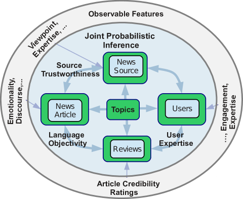
(a) Interactions between source trustworthiness, posting (i.e. article) credibility, language objectivity, and user expertise.

(b) Sample instantiation.

(c) Clique representation.

Figure III.2: Graphical model representation.

The earlier model is used for classifying statements as credible or not. However, in many scenarios for a more fine-grained credibility analysis, we want to assign a real-valued credibility rating to a posting. Additionally, we want to address several drawbacks of the earlier model, and propose a more general framework that models topics, users, sources, and explicit interactions between them — as is prevalent in any online community.

Refer to Figure III.2 for the following discussion. Consider a set of sources $\langle s\rangle$ (e.g., $s_{1}$ in Figure III.2(c)) generating postings $\langle p\rangle$ which are reviewed and analyzed by users $\langle u\rangle$ for their credibility. Consider $r_{ij}$ to be the review by user $u_{j}$ on posting $p_{i}$. The overall credibility rating of the posting $p_{i}$ is given by $y_{i}$.

In this model, each source, posting, user and her rating or review, and overall rating of the posting is associated with a continuous random variable $r.v.\in[1\ldots 5]$, that indicates its trustworthiness, objectivity, expertise, and credibility, respectively. $5$ indicates the best quality that an item can obtain, and $1$ is the worst. Discrete ratings, being a special case of this setting, can be easily handled.

Each node is associated with a set of observed features that are extracted from the community. For example, a source has properties like topic specific expertise, viewpoint and format of news; a posting has features like topics, and style of writing from the usage of discourse markers and subjective words in the posting. For users we extract their topical perspectives and expertise, engagement features (like the number of questions, replies, reviews posted) and various interactions with other users (like upvotes/downvotes) and sources in the community.

The objective of our model is to predict credibility ratings $\langle y\rangle$ of postings $\langle d\rangle$ by exploiting the mutual interactions between different variables. The following edges between the variables capture their interplay:

• Each posting is connected to the source from where it is extracted (e.g., $s_{1}-p_{1}$, $s_{1}-p_{2}$)

• Each posting is connected to its review or rating by a user (e.g., $p_{1}-r_{11}$, $p_{1}-r_{12}$, $p_{2}-r_{22}$)

• Each user is connected to all her reviews (e.g., $u_{1}-r_{11}$, $u_{2}-r_{12}$, $u_{2}-r_{22}$)

• Each user is connected to all postings rated by her (e.g., $u_{1}-p_{1}$, $u_{2}-p_{1}$, $u_{2}-p_{2}$)

• Each source is connected to all the users who rated its postings (e.g., $s_{1}-u_{1}$, $s_{1}-u_{2}$)

• Each source is connected to all the reviews of its postings (e.g., $s_{1}-r_{11}$, $s_{1}-r_{12}$, $s_{1}-r_{22}$)

• For each posting, all the users and all their reviews on the posting are inter-connected (e.g., $u_{1}-r_{12}$, $u_{2}-r_{11}$, $u_{1}-u_{2}$). This captures user-user interactions (e.g., $u_{1}$ upvoting/downvoting $u_{2}$’s rating on $p_{1}$) influencing the overall post rating.

Therefore, a clique (e.g., $C_{1}$) is formed between a posting, its source, users and their reviews on the posting. Multiple such cliques (e.g., $C_{1}$ and $C_{2}$) share information via their common sources (e.g., $s_{1}$) and users (e.g., $u_{2}$).

Topics play a significant role on information credibility. Individual users in community (and sources) have their own perspectives and expertise on various topics (e.g., environmental politics). Modeling user-specific topical perspectives explicitly captures credibility judgment better than a user-independent model. However, many postings do not have explicit topic tags. Hence we use Latent Dirichlet Allocation (LDA) [Blei 2001] in conjunction with Support Vector Regression (SVR) [Drucker 1996] to learn words associated to each (latent) topic, and user (and source) perspectives for the topics. Documents are assumed to have a distribution over topics as latent variables, with words as observables. Inference is by Gibbs sampling. This LDA model is a component of the overall model, discussed next.

We use a probabilistic graphical model, specifically a Conditional Random Field (CRF), to model all factors jointly. The modeling approach is related to the model discussed in the previous Section III.3.1. However, unlike that model and traditional CRF models, our problem setting requires a continuous version of the CRF (CCRF) to deal with real-valued ratings instead of discrete labels. In this work, we follow an approach similar to [Qin 2008, Radosavljevic 2010, Baltrusaitis 2014] in learning the parameters of the CCRF. We use Support Vector Regression [Drucker 1996] to learn the elements of the feature vector for the CCRF.

The inference is centered around cliques of the form $\langle$ source, posting, $\langle$ users $\rangle$, $\langle$ reviews $\rangle\rangle$. An example is the two cliques $C_{1}:\leavevmode\nobreak\ s_{1}-p_{1}-\langle u_{1},u_{2}\rangle-\langle r_{11},r_{12}\rangle$ and $C_{2}:\leavevmode\nobreak\ s_{1}-p_{2}-u_{2}-r_{22}$ in the instance graph of Figure III.2(c). This captures the “cross-talk” between different cliques sharing nodes. A source garners trustworthiness by generating multiple credible postings. Users attain expertise by correctly identifying credible postings that corroborate with other expert users. Inability to do so brings down their expertise. Similarly, a posting attains credibility if it is generated by a trustworthy source and highly rated by an expert user. The inference algorithm for the CCRF is discussed in detail in Section III.5.2.

In the following section, we discuss the various feature groups that are considered in our credibility model.

III.4 Model Components

In this section, we outline the different components, and features used in our probabilistic models for credibility analysis with a focus on health and news communities. These features are extracted from the postings of users in online communities, and their interactions with other users and sources. Since the features are fairly generic, and not community-specific — they are easily applicable to other communities like travel, food, and electronics.

III.4.1 Postings and their Language

The style in which a post is written plays a pivotal role in understanding its credibility. The desired property for a posting is to be objective and unbiased. In our model we use stylistic and affective features to assess a posting’s objectivity and quality.

Stylistic

Consider the following user posting in a health community:

Example III.4.1

“I heard Xanax can have pretty bad side-effects. You may have peeling of skin, and apparently some friend of mine told me you can develop ulcers in the lips also. If you take this medicine for a long time then you would probably develop a lot of other physical problems. Which of these did you experience ?”

This posting evokes a lot of uncertainty, and does not specifically point to the occurrence of any side effect from a first-hand experience. Note the usage of strong modals (depicting a high degree of uncertainty) “can”, “may”, “would”, the indefinite determiner “some”, the conditional “if”, the adverb of possibility “probably”, and the question particle “which”. Even the usage of too many named entities for drug and disease names can impact the credibility of a statement (refer the introductory Example III.1.2).

Contrast the above posting with the following one :

Example III.4.2

“Depo is very dangerous as a birth control and has too many long term side-effects like reducing bone density. Hence, I will never recommend anyone using this as a birth control. Some women tolerate it well but those are the minority. Most women have horrible long lasting side-effects from it.”

This posting uses the inferential conjunction “hence” to draw conclusions from a previous argument, the definite determiners “this”, “those”, “the” and “most” to pinpoint entities and the highly certain weak modal “will”.

Table III.1 shows a set of linguistic features which we deem suitable for discriminating between these two kinds of postings. Many of the features related to epistemic modality have been discussed in prior linguistic literature [Coates 1987, Westnet 2009] and features related to discourse coherence have also been employed in earlier computational work (e.g., [Mukherjee 2012, Wolf 2004]).

Feature types	Example values	Feature types	Example values
Strong modals	might, could, can, would	First person	I, we, me, my, mine, us, our
Weak modals	should, ought, need, shall	Second person	you, your, yours
Conditionals	if	Third person	he, she, him, her, his, it, its
Negation	no, not, neither, nor, never	Question particles	why, what, when, which
Inferential conj.	therefore, thus, furthermore	Adjectives	correct, extreme, visible
Contrasting conj.	until, despite, in spite	Adverbs	maybe, about, probably
Following conj.	but, however, otherwise, yet	Proper nouns	Xanax, Zoloft, Depo
Definite det.	the, this, that, those, these

Table III.1: Stylistic features.

Affective

Each user has an affective state that depicts her attitude and emotions that are reflected in her postings. Note that a user’s affective state may change over time; so it is a property of postings, not of users per se. As an example, consider the following posting in a health community:

Example III.4.3

“I’ve had chronic depression off and on since adolescence. In the past I’ve taken Paxil (made me anxious) and Zoloft (caused insomnia and stomach problems, but at least I was mellow ). I have been taking St. John’s Wort for a few months now, and it helps, but not enough. I wake up almost every morning feeling very sad and hopeless. As afternoon approaches I start to feel better, but there’s almost always at least a low level of depression throughout the day.”

The high level of depression and negativity in the posting makes one wonder if the statements on drug side-effects are really credible. Contrast this posting to the following one:

Example III.4.4

“A diagnosis of GAD (Generalized Anxiety Disorder) is made if you suffer from excessive anxiety or worry and have at least three symptoms including…If the symptoms above, touch a chord with you, do speak to your GP. There are effective treatments for GAD, and Cognitive Behavioural Therapy in particular can help you …”

— where the user objectivity and positivity in the posting make it much more credible.

We use the WordNet-Affect lexicon [Strapparava 2004], where each word sense (WordNet synset) is mapped to one of 285 attributes of the affective feature space, like confusion, ambiguity, hope, anticipation, hate. We do not perform word sense disambiguation (WSD), and instead simply take the most common sense of a word (which is generally a good heuristics for WSD). Table III.2 shows a sample of the affective features used in this work.

Sample Affective Features

affection, antipathy, anxiousness, approval, compunction, confidence, contentment, coolness, creeps, depression, devotion, distress, downheartedness, eagerness, edginess, embarrassment, encouragement, favor, fit, fondness, guilt, harassment, humility, hysteria, ingratitude, insecurity, jitteriness, levity, levitygaiety, malice, misery, resignation, selfesteem, stupefaction, surprise, sympathy, togetherness, triumph, weight, wonder

Table III.2: Examples of affective features.

Bias and Subjectivity

A posting is supposed to be objective: writers should not convey their own opinions, feelings or prejudices in their postings. For example, a posting titled “Why do conservatives hate your children?” is not considered objective journalism in a news community. We use the following linguistic cues for detecting bias and subjectivity in user-written postings. A subset of these features has been earlier used in [Recasens 2013, Mukherjee 2014b].

Assertives: Assertive verbs (e.g., “claim”) complement and modify a proposition in a sentence. They capture the degree of certainty to which a proposition holds.

Factives: Factive verbs (e.g., “indicate”) pre-suppose the truth of a proposition in a sentence.

Hedges: These are mitigating words (e.g., “may”) to soften the degree of commitment to a proposition.

Implicatives: These words trigger pre-supposition in an utterance. For example, usage of the word complicit indicates participation in an activity in an unlawful way.

Report verbs: These verbs (e.g., “argue”) are used to indicate the attitude towards the source, or report what someone said more accurately, rather than using just say and tell.

Discourse markers: These capture the degree of confidence, perspective, and certainty in the set of propositions made. For instance, strong modals (e.g., “could”), probabilistic adverbs (e.g., “maybe”), and conditionals (e.g., “if”) depict a high degree of uncertainty and hypothetical situations, whereas weak modals (e.g., “should”) and inferential conjunctions (e.g., “therefore”) depict certainty.

Subjectivity: We use a subjectivity lexicon, a list of positive and negative opinionated words, and an affective lexicon to detect subjective clues in postings.

We additionally harness a lexicon of bias-inducing words extracted from the Wikipedia edit history from [Recasens 2013] exploiting its Neutral Point of View Policy to keep its postings “fairly, proportionately, and as far as possible without bias, all significant views that have been published by reliable sources on a topic”.

Category	Example Values	#Count	Category	Example Values	#Count
Bias			Subjectivity
Assertives	think, believe, suppose, expect, imagine	66	Wiki Bias Lexicon	apologetic, summer, advance, cornerstone,	354
Factives	know, realize, regret, forget, find out	27	Negative	hypocricy, swindle, unacceptable, worse	4783
Hedges	postulates, felt, likely, mainly, guess	100	Positive	steadiest, enjoyed, prominence, lucky	2006
Implicatives	manage, remember, bother, get, dare	32	Subj. Clues	better, heckle, grisly, defeat, peevish	8221
Report	claim, underscore, alert, express, expect	181	Affective	disgust, anxious, revolt, guilt, confident	2978

Table III.3: Subjectivity and bias features.

Feature vector construction: For each stylistic feature type $f_{i}$ and each posting $p_{j}$, we compute the relative frequency of words of type $f_{i}$ occurring in $p_{j}$, thus constructing a feature vector $F^{L}(p_{j})=\langle freq_{ij}=\#(words\leavevmode\nobreak\ in\leavevmode\nobreak\ f_{i})\leavevmode\nobreak\ /\leavevmode\nobreak\ length(p_{j})\rangle$.

We further aggregate these vectors over all postings $p_{j}$ by a user $u_{k}$ into

$$F^{L}(u_{k})=\langle{\sum_{p_{j}\leavevmode\nobreak\ by\leavevmode\nobreak\ u_{k}}\#(words\leavevmode\nobreak\ in\leavevmode\nobreak\ f_{i})}\leavevmode\nobreak\ /\leavevmode\nobreak\ {\sum_{p_{j}\leavevmode\nobreak\ by\leavevmode\nobreak\ u_{k}}length(p_{j})}\rangle.$$ (III.1)

Since our model allows users to interact with other users, and give feedback (reviews/comments) on their postings — we also create feature vectors for the users’ reviews to capture whether the feedbacks are credible or biased by the users’ judgment. Consider the review $r_{j,k}$ written by user $u_{k}$ on a posting $p_{j}$. For each such review, analogous to the per-posting stylistic feature vector $\langle F^{L}(p_{j})\rangle$, we construct a per-review feature vector $\langle F^{L}(r_{j,k})\rangle$.

III.4.2 User Expertise

A user’s expertise in judging credibility of other users’ postings depends on many factors. [Einhorn 1977] discusses the following traits for recognizing an expert.

• An expert user needs to be recognized by other members.

• Experience is an uncertain indicator of user expertise.

• Inter-expert agreement should be high.

• Experts should be independent of bias.

Community Engagement: of the user is an obvious measure for judging the user authority in the community. We capture this with different features: number of answers, ratings given, comments, ratings received, disagreement and number of raters. In case user demography information like age, gender, location, etc. are available, we also incorporate them as features.

Inter-User Agreement: Expert users typically agree on what constitutes a credible posting. This is inherently captured in the proposed graphical model, where a user gains expertise by assigning credibility ratings to postings that corroborate with other expert users.

Topical Perspective and Expertise: The potential for harvesting user preference and expertise in topics for rating prediction of reviews has been demonstrated in [Mukherjee 2014a, McAuley 2013a]. For credibility analysis, the model needs to capture the user’s perspective and bias towards certain topics based on their political inclination that bias their ratings, and their topic-specific expertise that allows them to evaluate postings on certain topics better as “Subject Matter Experts”. These are captured as per-user feature weights for the stylistic indicators and topic words in the language of user-contributed reviews.

Interactions: In a community, users can upvote (digg, like, rate) the ratings of users that they appreciate, and downvote the ones they do not agree with. High review ratings from expert users increase the value of a user; whereas low ratings bring down her expertise. Similar to this user-user interaction, there can be user-posting, user-source and source-posting interactions which are captured as edges in our graphical model (by construction). Consider the following anecdotal example in the community showing an expert in nuclear energy downvoting another user’s rating on nuclear radiation:

Example III.4.5

“Non-expert: Interesting opinion about health risks of nuclear radiation, from a physicist at Oxford University. He makes some reasonable points …
Low rating by expert to above review: Is it fair to assume that you have no background in biology or anything medical? While this story is definitely very important, it contains enough inaccurate and/or misleading statements…”

Verbosity: Users who write long postings tend to deviate from the topic, often with highly emotional digression. On the other hand, short postings can be regarded as being crisp, objective and on topic. Specifically, we compute the first three moments of each user’s posting-length distribution, in terms of sentences and in terms of words.

Feature vector construction For each user $u_{k}$, we create an engagement feature vector $\langle F^{E}(u_{k})\rangle$. In order to capture user subjectivity, in terms of different stylistic indicators of credibility, we consider the per-review language feature vector $\langle F^{L}(r_{j,k})\rangle$ of user $u_{k}$ (refer to Section III.4.1). To capture user perspective and expertise on different topics, we consider the per-review topic feature vector $\langle F^{T}(r_{j,k})\rangle$ of each user $u_{k}$ (discussed in the next section).

III.4.3 Postings and their Topics

Topic tags for postings play an important role in user-perceived prominence, bias and credibility, in accordance to the Prominence-Interpretation theory [Fogg 2003]. For example, the tag Politics is often viewed as an indicator of potential bias and individual differences; whereas tags like Energy or Environment are perceived as more neutral postings and therefore invoke higher agreement in the community on the associated postings’ credibility. Obviously, this can be misleading as there is a significant influence of Politics on all topics.

Certain users have topic-specific expertise that make them judge (or rate) postings on those topics better than others. Sources also have expertise on specific topics and provide a better coverage of postings on those topics than others. For example, National Geographic provides a good coverage of postings related to environment, whereas The Wall Street Journal provides a good coverage on economic policies.

However, most postings do not have any explicit topic tag. In order to automatically identify the underlying theme of the posting, we use Latent Dirichlet Allocation (LDA) [Blei 2001] to learn the latent topic distribution in the corpus. LDA assumes a document to have a distribution over a set of topics, and each topic to have a distribution over words. Table III.4 shows an excerpt of the top topic words in each topic, where we manually added illustrative labels for the topics. The latent topics also capture some subtle themes not detected by the explicit tags. For example, Amy Goodman is an American broadcast journalist, syndicated columnist and investigative reporter who is considered highly credible in the community. Also, associated with that topic cluster is Amanda Blackhorse, a Navajo activist and plaintiff in the Washington Redskins case.

Feature vector construction: For each posting $p_{j}$ and each of its review $r_{j,k}$, we create feature vectors $\langle F^{T}(p_{j})\rangle$ and $\langle F^{T}(r_{j,k})\rangle$ respectively, using the learned latent topic distributions, as well as the explicit topic tags. Section III.5.2 discusses our method to learn the topic distributions.

Latent Topics	Topic Words
Obama admin.	obama, republican, party, election, president, senate, gop, vote
Citizen journ.	cjr, jouralism, writers, cjrs, marx, hutchins, reporting, liberty, guides
US military	iraq, war, military, iran, china, nuclear, obama, russia, weapons
AmyGoodman	democracy, military, civil, activist, protests, killing, navajo, amanda
Alternet	media, politics, world news, activism, world, civil, visions, economy
Climate	energy, climate, power, water, change, global, nuclear, fuel, warming

Table III.4: Latent topics (with illustrative labels) and their words.

III.4.4 Sources

A source is considered trustworthy if it generates highly credible postings. We examine the effect of different features of a source on its trustworthiness based on user assigned ratings in the community. We consider the following source features (summarized in Table III.5) for a news community: the type of media (e.g., online, newspaper, tv, blog), format of postings (e.g., news analysis, opinion, special report, news report, investigative report), (political) viewpoint (e.g., left, center, right), scope (e.g., international, national, local), the top topics covered by the source, and their topic-specific expertise.

Category	Elements
Media	newspaper, blog, radio, magazine, online
Format	editorial, investigative report, news, research
Scope	local, state, regional, national, international
Viewpoint	far left, left, center, right, neutral
Top Topics	politics, weather, war, science,, U.S. military
Expertise on Topics	U.S. congress, Middle East, crime, presidential election, Bush administration, global warming

Table III.5: Features for source trustworthiness.

Feature vector construction: For each source $s_{l}$, we create a feature vector $\langle F^{S}(s_{l})\rangle$ using features in Table III.5. Each element $f_{i}^{S}(s_{l})$ is $1$ or $0$ indicating presence or absence of a feature. Note that above features include the top (explicit) topics covered by any source, and its topic-specific expertise for a subset of those topics.

III.5 Probabilistic Inference

III.5.1 Semi-supervised Conditional Random Fields for Credibility Classification

Given a set of users (or sources) contributing postings containing dubious statements — in the first task, we want to classify the statements as credible or not. For instance, users in a health community can write postings about their experience with drugs and their side-effects, from where we want to extract the most credible side-effects of a given drug; sources can generate postings (i.e. articles) containing dubious claims, whereby we may be interested to find out if the claims are authentic or hoaxes.

We first propose a probabilistic model for classification with the following simplifications, which are addressed in Section III.5.2:

• We do not model users and sources separately as factors.

• We do not take into account inter user or inter source interactions.

• We no not model topics implicitly or explicitly, assuming all discussions are on a homogeneous topic (e.g., health).

As outlined in Section III.3, we model our learning task as a Markov Random Field (MRF), where the random variables are the users $U=\{u_{1},u_{2},...u_{|U|}\}$, their postings $P=\{p_{1},p_{2}...p_{|P|}\}$, and the distinct statements $S=\{s_{1},s_{2}...s_{|S|}\}$ extracted from all postings — whose credibility labels need to be inferred. For example, in a health community the statements are SPO (Subject-Predicate-Object) triples of the form ‘‘X_Causes_Y’’ ($X$: Drug, $Y$: Side-effect); in the open web the statements can be SPO claims like ‘‘Obama_BornIn_Kenya’’.

Our model is semi-supervised in that we harness ground-truth labels for a subset of statements, derived from the expert knowledge-bases. Let $S^{L}$ be the set of statements labeled by an expert as true or false, and let $S^{U}$ be the set of unlabeled statements. Our goal is to infer labels for the statements in $S^{U}.$

The cliques in our MRF are triangles consisting of a statement $s_{i}$, a posting $p_{j}$ that contains that statement, and a user $u_{k}$ who wrote this post. As the same statement can be made in different postings by the same or other users, there are more cliques than statements. For convenient notation, let $S^{*}$ denote the set of statement instances that correspond to the set of cliques, with statements “repeated” when necessary.

Let $\phi_{i}(S^{*}_{i},p_{j},u_{k})$ be a potential function for clique $i$. Each clique has a set of associated feature functions $F_{i}$ with a weight vector $W$. We denote the individual features and their weights as $f_{il}$ and $w_{l}$. The features are constituted by the stylistic, affective, and user features explained in Section III.4: $F_{i}=F^{L}(p_{j})\cup F^{E}(p_{j})\cup F^{U}(u_{k}).$

Instead of computing the joint probability distribution $Pr(S,P,U;W)$ like in a standard MRF, we adopt the paradigm of Conditional Random Fields (CRF’s) and settle for the simpler task of estimating the conditional distribution:

$$Pr(S|P,U;W)=\frac{1}{Z(P,U)}\prod_{i}\phi_{i}(S^{*}_{i},p_{j},u_{k};W),$$ (III.2)

with normalization constant $Z(P,U)$;

or with features and weights made explicit:

$$Pr(S|P,U;W)=\frac{1}{Z(P,U)}\prod_{i}\exp(\sum_{l}w_{l}\times f_{il}(S^{*}_{i},p_{j},u_{k})).$$ (III.3)

CRF parameter learning usually works on fully observed training data. However, in our setting, only a subset of the $S$ variables have labels and we need to consider the partitioning of $S$ into $S^{L}$ and $S^{U}$:

$$Pr(S^{U},S^{L}|P,U;W)=\frac{1}{Z(P,U)}\prod_{i}\exp(\sum_{l}w_{l}\times f_{il}(S^{*}_{i},p_{j},u_{k})).$$ (III.4)

For parameter estimation, we need to maximize the marginal log-likelihood:

$$LL(W)=\log Pr(S^{L}|Ps,U;W)=\log\sum_{S^{U}}Pr(S^{L},S^{U}|P,U;W).$$ (III.5)

We can clamp the values of $S^{L}$ to their observed values in the training data [Sutton 2012, Zhu 2003] and compute the distribution over $S^{U}$ as:

$$Pr(S^{U}|S^{L},P,U;W)=\frac{1}{Z(S^{L},P,U)}\prod_{i}\exp(\sum_{l}w_{l}\times f_{il}(S^{*}_{i},p_{j},u_{k})).$$ (III.6)

There are different ways of addressing the optimization problem for finding the argmax of $LL(W)$. In this work, we choose the Expectation-Maximization (EM) approach [McCallum 2005]. We first estimate the labels of the variables $S^{U}$ from the posterior distribution using Gibbs sampling, and then maximize the log-likelihood to estimate the feature weights:

$$E-Step:q(S^{U}) =Pr(S^{U}|S^{L},P,U;W^{(\nu)})$$ (III.7a)

$$M-Step:W^{(\nu+1)} =argmax_{W^{\prime}}\sum_{S^{U}}q(S^{U})\log Pr(S^{L},S^{U}|P,U;W^{\prime}).$$ (III.7b)

The update step to sample the labels of $S^{U}$ variables by Gibbs sampling is given by:

$$Pr(S^{U}_{i}|P,U,S^{L};W)\propto\prod_{\nu\in C}\phi_{\nu}(S^{*}_{\nu},p_{j},u_{k};W),$$ (III.8)

where $C$ denotes the set of cliques containing statement $S^{U}_{i}$.

For the M-step in Equation III.7b, we use an $L_{2}$-regularized Trust Region Newton Method [Lin 2008], suited for large-scale unconstrained optimization, where many feature values may be zero. For this we use an implementation of LibLinear [Fan 2008].

The above approach captures user trustworthiness implicitly via the weights of the feature vectors. However, we may want to model user trustworthiness in a way that explicitly aggregates over all the statements made by a user. Let $t_{k}$ denote the trustworthiness of user $u_{k}$, measured as the fraction of her statements that were considered true in the previous EM iteration:

$$t_{k}=\frac{\sum_{i}\mathbf{1}_{S_{i,k}=\mbox{True}}}{|S_{k}|},$$ (III.9)

where $S_{i,k}$ is the label assigned to $u_{k}$’s statement $S_{i}$ in the previous EM iteration. Equation III.8 can then be modified into:

$$Pr(S^{U}_{i}|P,U,S^{L};W)\propto\prod_{\nu\in C}t_{k}\times\phi_{\nu}(S^{*}_{\nu},p_{j},u_{k};W)$$ (III.10)

Therefore, the random variable for trustworthiness depends on the proportion of true statements made by the user. The label of a statement, in turn, is determined by the language objectivity of the postings and trustworthiness of all the users in the community that make the statement.

The inference is an iterative process consisting of the following $3$ main steps:

• Estimate user trustworthiness $t_{k}$ using Equation III.9.

• Apply the E-Step to estimate $q(S^{U};W^{(\nu)})$
  For each $i$, sample $S_{i}^{U}$ from Equation III.7a and III.10.

• Apply the M-Step to estimate $W^{(\nu+1)}$ using Equation III.7b.

III.5.2 Continuous Conditional Random Fields for Credibility Regression

In the previous section, we discussed an approach for classifying statements as credible or not. However, in many scenarios we want to perform a more fine-grained analysis. Some communities (e.g., newstrust.net) offer users fine-grained scales for rating different aspects of an item — which are aggregated into an overall real-valued rating after weighing the aspects based on their importance, expertise of the user, feedback from the community, and more. This setting cannot be easily discretized without blowup or risking to lose information. Therefore, in this task we want to perform regression for fine-grained credibility analysis, whereby we want to assign a real-valued credibility rating (e.g. $2.5$ on a scale of $1$ to $5$) to a posting.

We also address the earlier drawbacks of our model (discussed in Section III.5.1), whereby we now model users and sources as separate factors, taking into consideration the inter user and inter source interactions, as well as the influence of topics of discussions.

Consider a set of sources generating postings (i.e. articles), and a set of users providing feedback (i.e. writing reviews) on the postings with mutual interactions (i.e. a user can upvote/downvote, like, and share other users’ reviews) — our objective is to identify credible postings, trustworthy sources, and expert users jointly in the community, incorporating the discussed features and insights (discussed in Section III.4).

Table III.6 summarizes the important notations used in this section.

Variables	Type	Description
$p_{j}$	Vector	Document with sequence of words $\langle w\rangle$
$s$	Vector	Sources
$u$	Vector	Users
$r_{j,k}$	Vector	Review by user $u_{k}$ on document $p_{j}$
		with sequence of words $\langle w\rangle$
$y_{j,k}$	Real Number	Rating of $r_{j,k}$
$z$	Vector	Sequence of topic assignments for $\langle w\rangle$
$\text{SVR}_{u_{k}},\text{SVR}_{s_{i}}$	Real Number	SVR prediction for users, sources,
$\text{SVR}_{L},\text{SVR}_{T}$	$\in$ [1 …5]	language, and topics
$\Psi=f(\langle\psi_{j}\rangle)$	Real Number	Clique potential with $\psi_{j}=\langle y_{j},s_{i},p_{j},$ $\langle u_{k}\rangle,\langle r_{j,k}\rangle\rangle$ for clique of $p_{j}$
${\lambda=}$ $\langle\alpha_{u},\beta_{s},\gamma_{1},\gamma_{2}\rangle$	Vector	Combination weights for users $\langle u\rangle$, sources $\langle s\rangle$, language and topic models
$y_{n\times 1}$	Vector	Credibility rating of documents $\langle d\rangle$
$X_{n\times m}$	Matrix	Feature matrix with $m=|U|+|S|+2$
$Q_{n\times n}$	Diagonal Matrix	$f(\lambda)$
$b_{n\times 1}$	Vector	$f(\lambda,X)$
$\Sigma_{n\times n}$	CovarianceMatrix	$f(\lambda)$
$\mu_{n\times 1}$	Mean Vector	$f(\lambda,X)$

Table III.6: Symbol table.

Topic Model

Consider a posting $d$ consisting of a sequence of $\{N_{d}\}$ words denoted by ${w_{1},w_{2},...w_{N_{d}}}$. Each word is drawn from a vocabulary $V$ having unique words indexed by ${1,2,...V}$. Consider a set of topic assignments $z=\{z_{1},z_{2},...z_{K}\}$ for $d$, where each topic $z_{i}$ can be from a set of $K$ possible topics.

LDA [Blei 2001] assumes each document $d$ to be associated with a multinomial distribution $\theta_{d}$ over topics $Z$ with a symmetric dirichlet prior $\rho$. $\theta_{d}(z)$ denotes the probability of occurrence of topic $z$ in document $d$. Topics have a multinomial distribution $\phi_{z}$ over words drawn from a vocabulary $V$ with a symmetric dirichlet prior $\zeta$. $\phi_{z}(w)$ denotes the probability of the word $w$ belonging to the topic $z$. Exact inference is not possible due to intractable coupling between $\Theta$ and $\Phi$. We use Gibbs sampling for approximate inference.

Let $n(d,z,w)$ denote the count of the word $w$ occurring in document $d$ belonging to the topic $z$. In the following equation, $(.)$ at any position in the above count indicates marginalization, i.e., summing up the counts over all values for the corresponding position in $n(d,z,w)$. The conditional distribution for the latent variable $z$ (with components $z_{1}$ to $z_{K}$) is given by:

$$P(z_{i}=k| w_{i}=w,z_{-i},w_{-i})\propto$$ (III.11)

$$\frac{n(d,k,.)+\rho}{\sum_{k}n(d,k,.)+K\rho} \times\frac{n(.,k,w)+\zeta}{\sum_{w}n(.,k,w)+V\zeta}$$

Let $\langle T^{E}\rangle$ and $\langle T^{L}\rangle$ be the set of explicit topic tags and latent topic dimensions, respectively. The topic feature vector $\langle F^{T}\rangle$ for a posting or review combines both explicit tags and latent topics and is constructed as follows:

$$F^{T}_{t}(d)=\begin{cases}\#freq(w,d),&\text{if}\ T^{E}_{t^{{}^{\prime}}}=F^{T}_{t}\\ \#freq(w,d)\times\phi_{T^{L}_{{t^{\prime}}}}(w),&\text{if}\ T^{L}_{t^{{}^{\prime}}}=F^{T}_{t}\text{ and }\phi_{T^{L}_{t^{{}^{\prime}}}}(w)>\delta\\ 0&\text{otherwise}\end{cases}\hfill$$

So for any word in the document matching an explicit topic tag, the corresponding element in the feature vector $\langle F^{T}\rangle$ is set to its occurrence count in the document. If the word belongs to any latent topic with probability greater than threshold $\delta$, the probability of the word belonging to that topic ($\phi_{t}(w)$) is added to the corresponding element in the feature vector, and set to $0$ otherwise.

Support Vector Regression

We use Support Vector Regression (SVR) [Drucker 1996] to combine the different features discussed in Section III.4. SVR is an extension of the max-margin framework for SVM classification to the regression problem. It solves the following optimization problem to learn weights $w$ for features $F$:

$$\min_{w}\frac{1}{2}{w}^{T}{w}+C\times\sum_{d=1}^{N}(max(0,|y_{d}-w^{T}F|-\epsilon))^{2}\hfill$$ (III.12)

Posting Stylistic Model: We learn a stylistic regression model $\text{SVR}_{L}$ using the per-posting stylistic feature vector $\langle F^{L}(p_{j})\rangle$ for posting $p_{j}$ (or, $\langle F^{L}(r_{j,k})\rangle$ for review $r_{j,k}$), with the overall credibility rating $y_{j}$ (or, $y_{j,k}$) of the posting as the response variable.

Posting Topic Model: Similarly, we learn a topic regression model $\text{SVR}_{T}$ using the per-posting topic feature vector $\langle F^{T}(p_{j})\rangle$ for posting $p_{j}$ (or, $\langle F^{T}(r_{j,k})\rangle$ for review $r_{j,k}$), with the overall credibility rating $y_{j}$ (or, $y_{j,k}$) of the posting as the response variable.

Source Model: We learn a source regression model $\text{SVR}_{s_{i}}$ using the per-source feature vector $\langle F^{S}(s_{i})\rangle$ for source $s_{i}$, with the overall source rating as the response variable .

User Model: For each user $u_{k}$, we learn a user regression model $\text{SVR}_{u_{k}}$ with her per-review stylistic and topic feature vectors
$\langle F^{L}(r_{j,k})\cup F^{T}(r_{j,k})\rangle$ for review $r_{j,k}$ for posting $p_{j}$, with her overall review rating $y_{j,k}$ as the response variable.

Note that we use overall credibility rating of the posting to train posting stylistic and topic models. For the user model, however, we take user assigned credibility ratings of the postings, and per-user features. This model captures user subjectivity and topic perspective. The source models are trained on source specific meta-data and its ground-truth ratings.

Continuous Conditional Random Field

We model our learning task as a Conditional Random Field (CRF), where the random variables are the ratings of postings $\langle p_{j}\rangle$, sources $\langle s_{i}\rangle$, users $\langle u_{k}\rangle$, and reviews $\langle r_{j,k}\rangle$. The objective is to predict the credibility ratings $\langle y_{j}\rangle$ of the postings $\langle p_{j}\rangle$.

The cliques in the CRF consist of a posting $p_{j}$, its source $s_{i}$, set of users $\langle u_{k}\rangle$ reviewing it, and the corresponding user reviews $\langle r_{j,k}\rangle$ — where $r_{j,k}$ denotes the review by user $u_{k}$ on posting $p_{j}$. Different cliques are connected via the common sources, and users. There are as many cliques as the number of postings.

Let $\psi_{j}(y_{j},s_{i},p_{j},\langle u_{k}\rangle,\langle r_{j,k}\rangle)$ be a potential function for clique $j$. Each clique has a set of associated vertex feature functions. In our problem setting, we associate features to each vertex. The features constituted by the stylistic, topic, source and user features explained in Section III.3.2 are: $F^{L}(p_{j})\cup F^{T}(p_{j})\cup F^{S}(s_{i})\cup_{k}(F^{E}(u_{k})\cup F^{L}(r_{j,k})\cup F^{T}(r_{j,k})).$

A traditional CRF model allows us to have a binary decision if a posting is credible ($y_{j}=1$) or not ($y_{j}=0$), by estimating the conditional distribution with the probability mass function of the discrete random variable $y$:

$$Pr(y|D,S,U,R)=\frac{\prod_{j=1}^{n}exp(\psi_{j}(y_{j},s_{i},p_{j},\langle u_{k}\rangle,\langle r_{j,k}\rangle))}{{\sum_{y}\prod_{j=1}^{n}exp(\psi_{j}(y_{j},s_{i},p_{j},\langle u_{k}\rangle,\langle r_{j,k}\rangle))}}$$ (III.13)

But in our problem setting, we want to estimate the credibility rating of a posting. Therefore, we need to estimate the conditional distribution with the probability density function of the continuous random variable $y$:

$$Pr(y|D,S,U,R)=\frac{\prod_{j=1}^{n}exp(\psi_{j}(y_{j},s_{i},p_{j},\langle u_{k}\rangle,\langle r_{j,k}\rangle))}{\int_{-\infty}^{\infty}\prod_{j=1}^{n}exp(\psi_{j}(y_{j},s_{i},p_{j},\langle u_{k}\rangle,\langle r_{j,k}\rangle))dy}\\$$ (III.14)

Given a posting $p_{j}$, its source id $s_{i}$, and a set of user ids $\langle u_{k}\rangle$ who reviewed the posting, the regression models $\text{SVR}_{L}(p_{j})$, $\text{SVR}_{T}(p_{j})$, $\text{SVR}_{s_{i}}$, $\langle\text{SVR}_{u_{k}}(p_{j})\rangle$ (discussed in Section III.5.2) independently predict the rating of $p_{j}$. For notational brevity, hereafter, we drop the argument $p_{j}$ from the SVR function. These SVR predictors are for separate feature groups and independent of each other. Now we combine the different SVR models to capture mutual interactions, such that the weight for each SVR model reflects our confidence on its quality. Errors by an SVR are penalized by the squared loss between the predicted credibility rating of the posting and the ground-truth rating. There is an additional constraint that for any clique only the regression models corresponding to the source and users present in it should be activated. This can be thought of as partitioning the input feature space into subsets, with the features inside a clique capturing local interactions, and the global weights capture the overall quality of the random variables via the shared information between the cliques (in terms of common sources, users, topics and language features) — an ideal setting for using a CRF. Equation III.15 shows one such linear combination. Energy function of an individual clique is given by:

$$\psi(y,s,d,\langle u\rangle,\langle r\rangle)=-\sum_{u}\alpha_{u}\mathbb{I}_{u}(d)(y-\text{SVR}_{u})^{2}\\ -\sum_{s}\beta_{s}\mathbb{I}_{s}(d)(y-\text{SVR}_{s})^{2}-\gamma_{1}(y-\text{SVR}_{L})^{2}-\gamma_{2}(y-\text{SVR}_{T})^{2}$$ (III.15)

Indicator functions $\mathbb{I}_{u_{k}}(p_{j})$ and $\mathbb{I}_{s_{i}}(p_{j})$ are 1 if $u_{k}$ is a reviewer and $s_{i}$ is the source of posting $p_{j}$ respectively, and are $0$ otherwise.

As the output of the SVR is used as an input to the CCRF in Equation III.15, each element of the input feature vector is already predicting the output variable. The learned parameters $\lambda=\langle\alpha,\beta,\gamma_{1},\gamma_{2}\rangle$ (with dimension$(\lambda)=|U|+|S|+2$) of the linear combination of the above features depict how much to trust individual predictors. Large $\lambda_{k}$ on a particular predictor places large penalty on the mistakes committed by it, and therefore depicts a higher quality for that predictor. $\alpha_{u}$ corresponding to user $u$ can be taken as a proxy for that user’s expertise, allowing us to obtain a ranked list of expert users. Similarly, $\beta_{s}$ corresponding to source $s$ can be taken as a proxy for that source’s trustworthiness, allowing us to obtain a ranked list of trustworthy sources.

Overall energy function of all cliques is given by:

$$\hskip 11.38092pt\hskip 11.38092pt\hskip 11.38092pt\hskip 11.38092pt\Psi=\sum_{j=1}^{n}\psi_{j}(y_{j},s_{i},p_{j},\langle u_{k}\rangle,\langle r_{j,k}\rangle)\\ \text{\normalsize(Substituting $\psi_{j}$ from Equation\leavevmode\nobreak\ \ref{eq.7} and re-organizing terms)}\\ \Psi=\sum_{j=1}^{n}(-\sum_{k=1}^{k=U}\alpha_{k}\mathbb{I}_{u_{k}}(p_{j})(y_{j}-\text{SVR}_{u_{k}})^{2}\\ -\sum_{i=1}^{i=S}\beta_{i}\mathbb{I}_{s_{i}}(p_{j})(y_{j}-\text{SVR}_{s_{i}})^{2}-\gamma_{1}(y_{j}-\text{SVR}_{L})^{2}-\gamma_{2}(y_{j}-\text{SVR}_{T})^{2})\\ =-\sum_{j=1}^{n}y_{j}^{2}[\sum_{k=1}^{k=U}\alpha_{k}\mathbb{I}_{u_{k}}(p_{j})+\sum_{i=1}^{i=S}\beta_{i}\mathbb{I}_{s_{i}}(p_{j})+\gamma_{1}+\gamma_{2}]\\ +\sum_{j=1}^{n}2y_{j}[\sum_{k=1}^{k=U}\alpha_{k}\mathbb{I}_{u_{k}}(p_{j})\text{SVR}_{u_{k}}+\sum_{i=1}^{i=S}\beta_{i}\mathbb{I}_{s_{i}}(p_{j})\text{SVR}_{s_{i}}+\gamma_{1}\text{SVR}_{L}+\gamma_{2}\text{SVR}_{T}]\\ -\sum_{j=1}^{n}[\sum_{k=1}^{k=U}\alpha_{k}\mathbb{I}_{u_{k}}(p_{j})\text{SVR}_{u_{k}}^{2}+\sum_{i=1}^{i=S}\beta_{i}\mathbb{I}_{s_{i}}(p_{j})\text{SVR}_{s_{i}}^{2}+\gamma_{1}\text{SVR}_{L}^{2}+\gamma_{2}\text{SVR}_{T}^{2}]\\$$

$$\text{\normalsize Organizing the bracketed terms into variables as follows:}\\ Q_{i,j}=\begin{cases}\sum_{k=1}^{k=U}\alpha_{k}\mathbb{I}_{u_{k}}(p_{i})+\sum_{l=1}^{l=S}\beta_{l}\mathbb{I}_{s_{l}}(p_{i})+\gamma_{1}+\gamma_{2}&i=j\\ 0&\ i\neq j\end{cases}\\ b_{i}=2[\sum_{k=1}^{k=U}\alpha_{k}\mathbb{I}_{u_{k}}(p_{i})\text{SVR}_{u_{k}}+\sum_{l=1}^{l=S}\beta_{l}\mathbb{I}_{s_{l}}(p_{i})\text{SVR}_{s_{l}}+\gamma_{1}\text{SVR}_{L}+\gamma_{2}\text{SVR}_{T}]\\ c=\sum_{j=1}^{n}[\sum_{k=1}^{k=U}\alpha_{k}\mathbb{I}_{u_{k}}(p_{j})\text{SVR}_{u_{k}}^{2}+\sum_{i=1}^{i=S}\beta_{i}\mathbb{I}_{s_{i}}(p_{j})\text{SVR}_{s_{i}}^{2}+\gamma_{1}\text{SVR}_{L}^{2}+\gamma_{2}\text{SVR}_{T}^{2}]\\$$

We can derive:

$$\@add@centering\centering\Psi=-y^{T}Qy+y^{T}b-c\hfill$$ (III.16)

Substituting $\Psi$ in Equation IV.3.4:

$$\begin{split}P(y|X)&=\frac{\prod_{j=1}^{n}exp(\psi_{j})}{\int_{-\infty}^{\infty}\prod_{j=1}^{n}exp(\psi_{j})dy}\\ &=\frac{exp(\Psi)}{\int_{-\infty}^{\infty}exp(\Psi)dy}\\ &=\frac{exp(-y^{T}Qy+y^{T}b)}{\int_{-\infty}^{\infty}exp(-y^{T}Qy+y^{T}b)dy}\\ &=\frac{exp(-\frac{1}{2}y^{T}\Sigma^{-1}y+y^{T}\Sigma^{-1}\mu)}{\int_{-\infty}^{\infty}exp(-\frac{1}{2}y^{T}\Sigma^{-1}y+y^{T}\Sigma^{-1}\mu)dy}\text{\hskip 11.38092pt\hskip 11.38092pt\hskip 11.38092pt{\normalsize(Substituting $Q=\frac{1}{2}\Sigma^{-1},b=\Sigma^{-1}\mu$)}}\end{split}$$ (III.17)

Equation III.17 can be transformed into a multivariate Gaussian distribution after substituting $\int_{-\infty}^{\infty}exp(-\frac{1}{2}y^{T}\Sigma^{-1}y+y^{T}\Sigma^{-1}\mu)dy=\frac{(2\pi)^{n/2}}{|\Sigma^{-1}|^{\frac{1}{2}}}exp(\frac{1}{2}\mu^{T}\Sigma^{-1}\mu)$. Therefore obtaining,

$$P(y|X)=\frac{1}{{(2\pi)}^{\frac{n}{2}}{|\Sigma|}^{\frac{1}{2}}}exp(-\frac{1}{2}(y-\mu)^{T}\Sigma^{-1}(y-\mu))\hfill$$ (III.18)

$Q$ represents the contribution of $\lambda$ to the covariance matrix $\Sigma$. Each row of the vector $b$ and matrix $Q$ corresponds to one training instance, representing the active contribution of features present in it. To ensure Equation III.18 represents a valid Gaussian distribution, the covariance matrix $\Sigma$ needs to be positive definite for its inverse to exist. For that the diagonal matrix $Q$ needs to be a positive semi-definite matrix. This can be ensured by making all the diagonal elements in $Q$ greater than $0$, by constraining $\lambda_{k}>0$.

Since this is a constrained optimization problem, gradient ascent cannot be directly used. We follow the approach similar to [Radosavljevic 2010] and maximize log-likelihood with respect to $log\ \lambda_{k}$, instead of $\lambda_{k}$ as in standard gradient ascent, making the optimization problem unconstrained as:

$$\frac{\partial logP(y|X)}{\partial log\lambda_{k}}=\alpha_{k}(\frac{\partial logP(y|X)}{\partial\lambda_{k}})\hfill$$ (III.19)

Taking partial derivative of the $log$ of Equation III.18 w.r.t $\lambda_{k}$:

$$\frac{\partial logP(y|X)}{\partial\lambda_{k}}=\frac{1}{2}\frac{\partial}{\partial\lambda_{k}}(-y^{T}\Sigma^{-1}y+2y^{T}\Sigma^{-1}\mu-\mu^{T}\Sigma^{-1}\mu+log|\Sigma^{-1}|+Constant)\hfill$$ (III.20)

Substituting the following in the above equation:

$$\centering\begin{split}\frac{\partial\Sigma^{-1}}{\partial\lambda_{k}}&=2\frac{\partial Q}{\partial\lambda_{k}}\\ &=2I\\ \frac{\partial\Sigma^{-1}\mu}{\partial\lambda_{k}}&=\frac{\partial b}{\partial\lambda_{k}}\ \ [\because\mu=\Sigma b]\\ &=2X_{(.),k}\text{\normalsize\hskip 30.00005pt where, $X_{(.),k}$ indicates the $k^{th}$ column of the feature matrix $X$.}\end{split}\@add@centering$$

$$\begin{split}\frac{\partial\Sigma}{\partial\lambda_{k}}&=-\Sigma\frac{\partial\Sigma^{-1}}{\partial\lambda_{k}}\Sigma\\ &=-2\Sigma\Sigma\\ \frac{\partial}{\partial\lambda_{k}}(\mu^{T}\Sigma^{-1}\mu)&=\frac{\partial}{\partial\lambda_{k}}(b^{T}\Sigma b)\\ &=b^{T}\frac{\partial\Sigma b}{\partial\lambda_{k}}+\frac{\partial b^{T}}{\partial\lambda_{k}}\Sigma b\\ &=b^{T}(\Sigma\frac{\partial b}{\partial\lambda_{k}}+\frac{\partial\Sigma}{\partial\lambda_{k}}b)+\frac{\partial b^{T}}{\partial\lambda_{k}}\Sigma b\\ &=4X_{(.),k}\Sigma b-2b^{T}\Sigma\Sigma b\\ &=4X_{(.),k}\mu-2\mu^{T}\mu\\ \frac{\partial log|\Sigma^{-1}|}{\partial\lambda_{k}}&=\frac{1}{|\Sigma^{-1}|}\text{Trace}(|\Sigma^{-1}|\Sigma\frac{\partial\Sigma^{-1}}{\partial\lambda_{k}})\\ &=2\text{Trace}(\Sigma)\hfill\end{split}$$

We can derive the gradient vector:

$$\frac{\partial logP(y|X)}{\partial\lambda_{k}}=-y^{T}y+2y^{T}X_{(.),k}-2X^{T}_{(.),k}\mu+\mu^{T}\mu+\text{Trace}(\Sigma)$$ (III.21)

Let $\eta$ denote the learning rate. The update equation is given by:

$$\centering log\lambda_{k}^{new}=log\lambda_{k}^{old}+\eta\frac{\partial logP(y|X)}{\partial log\lambda_{k}}\@add@centering$$ (III.22)

Once the model parameters are learned using gradient ascent, the inference for the prediction $y$ of the credibility rating of the posting is straightforward. As we assume the distribution to be Gaussian, the prediction is the expected value of the function, given by the mean of the distribution: $y\prime=argmax_{y}\ P(y|X)=\mu=\Sigma b$.
Note that $\Sigma$ and $b$ are both a function of $\lambda=\langle\alpha,\beta,\gamma_{1},\gamma_{2}\rangle$ which represents the combination weights of various factors to capture mutual interactions. The optimization problem determines the optimal $\lambda$ for reducing the error in prediction.

III.6 Experimental Evaluation: Health Communities

In this section, we apply the predictive power of our probabilistic model for classification (refer to Section III.5.1) to the problem of extracting credible side-effects of medical drugs from user-contributed postings in online healthforums.

III.6.1 Data

We use data from the healthboards.com, one of the largest online health communities, with $850,000$ registered members and over $4.5$ million posted messages. We sampled $15,000$ users based on their posting frequency and all of their postings, $2.8$ million postings in total for experimentation. Table III.7 shows the user categorization in terms of their community engagement. We employ an IE tool [Ernst 2014] to extract side-effect statements from the postings. It generates tens of thousands of such SPO triple patters, although only a handful of them are credible ones. Details of the experimental setting are available on our website.

Member Type	Members	Postings	Average Qs.	Average Replies
Administrator	1	-	363	934
Moderator	4	-	76	1276
Facilitator	16	> 4700	83	2339
Senior veteran	966	> 500	68	571
Veteran	916	> 300	41	176
Senior member	4321	> 100	24	71
Member	5846	> 50	13	28
Junior member	1423	> 40	9	18
Inactive	1433	-	-	-
Registered user	70	-	-	-

Table III.7: User statistics.

As ground truth for drug side-effects, we rely on data from the Mayo Clinic portal, which contains curated expert information about drugs, with side-effects being listed as more common, less common and rare for each drug. We extracted $2,172$ drugs which are categorized into $837$ drug families. For our experiments, we select $6$ widely used drug families (based on webmd.com). Table III.8 provides information on this sample and its coverage on healthboards.com. Table III.9 shows the number of common, less common, and rare side-effects for the six drug families as given by the Mayo Clinic portal.

III.6.2 Baselines

We compare our probabilistic model against the following baseline methods, using the same set of features for all the models, and classifying the same set of side-effect candidates.

Drugs	Description	Users	Postings
alprazolam, niravam, xanax	relieve symptoms of anxiety, depression, panic disorder	2785	21,112
ibuprofen, advil, genpril, motrin, midol, nuprin	relieve pain, symptoms of arthritis, such as inflammation, swelling, stiffness, joint pain	5657	15,573
omeprazole, prilosec	treat acidity in stomach, gastric and duodenal ulcers, …	1061	3884
metformin, glucophage, glumetza, sulfonylurea	treat high blood sugar levels, sugar diabetes	779	3562
levothyroxine, tirosint	treat hypothyroidism: insufficient hormone production by thyroid gland	432	2393
metronidazole, flagyl	treat bacterial infections in different body parts	492	1559

Table III.8: Information on sample drug families: number of postings and number of users reporting at least one side effect.

Drug family	Common	Less common	Rare
alprazolam	35	91	45
ibuprofen	30	1	94
omeprazole	-	15	20
metformin	24	37	5
levothyroxine	-	51	7
metronidazole	35	25	14

Table III.9: Number of common, less common, and rare side-effects listed by experts on Mayo Clinic.

Frequency Baseline: For each statement on a drug side-effect, we consider how frequently the statement has been made in community. This gives us a ranking of side-effects.

SVM Baseline: For each drug and possible side-effect we determine all postings where it is mentioned and aggregate the features $F^{L}$, $F^{E}$, $F^{U}$, described in Section III.4 over all these postings, thus creating a single feature vector for each side-effect.

We use the ground-truth labels from the Mayo Clinic portal to train a Support Vector Machine (SVM) classifier with a linear kernel, $L_{2}$ loss, and $L_{1}$ or $L_{2}$ regularization, for classifying unlabeled statements.

SVM Baseline with Distant Supervision: As the number of common side-effects for any drug is typically small, the above approach to create a single feature vector for each side-effect results in a very small training set. Hence, we use the notion of distant supervision to create a rich, expanded training set.

A feature vector is created for every mention or instance of a side-effect in different user postings. The feature vector $<S_{i},p_{j},u_{k}>$ has the label of the side-effect, and represents the set of cliques in Equation III.2. The semi-supervised CRF formulation in our approach further allows for information sharing between the cliques to estimate the labels of the unobserved statements from the expert-provided ones.

This process creates a noisy training set, as a posting may contain multiple side-effects, positive and negative. This results in multiple similar feature vectors with different labels. During testing, the same side-effect may get different labels from its different instances. We take a majority voting of the labels obtained by a side-effect, across predictions over its different instances, and assign a unique label to it.

III.6.3 Experiments and Quality Measures

We conduct two lines of experiments, with different settings on what is considered ground-truth.

Experimental Setting I: We consider only most common side-effects listed by the Mayo Clinic portal as positive ground-truth, whereas all other side-effects (less common, rare and unobserved) are considered to be negative instances (i.e., so unlikely that they should be considered as false statements, if reported by a user). The training set is constructed in the same way. This setting aims to study the predictive power of our model in determining the common side-effects of a drug, in comparison to the baselines.

Experimental Setting II: Here we address our original motivation: discovering less common and rare side-effects. Durring training, as positive ground-truth we consider common and less common side-effects (as stated by the experts on the Mayo Clinic site), whereas all rare and unobserved side-effects are considered negative instances. Our goal here is to test how well the model can identify less known and rare side-effects as true statements. We purposely do not consider rare side-effects as positive training examples, since we aim to evaluate the model’s ability to retrieve such statements starting only from very reliable positive instances. We measure performance on rare side-effects as the recall for such statements being labeled as true statements, in spite of considering only common and less common side-effects as positive instances durring training.

Train-Test Data Split: For each drug family, we create multiple random splits of $80\%$ training data and $20\%$ test data. All results reported below are averaged over $200$ such splits. All baselines and our CRF model use same test sets.

Evaluation Metrics: The standard measure for the quality of a binary classifier is accuracy: $\frac{tp+tn}{tp+fn+tn+fp}$. We also report the specificity ($\frac{tn}{tn+fp}$) and sensitivity ($\frac{tp}{tp+fn}$). Sensitivity measures the true positive rate or the model’s ability to identify positive side-effects, whereas specificity measures true negative rate.

III.6.4 Results and Discussions

Table III.10 shows the accuracy comparison of our system (CRF) with the baselines for different drug families in the first setting. The first naive baseline, which simply considers the frequency of postings containing the side-effect by different users, has an average accuracy of $57.65\%$ across different drug families.

Incorporating supervision in the classifier as the first SVM baseline (SVM w/o DS), along with a rich set of features for users, postings and language, achieves an average accuracy improvement of $11.4\%$. In the second SVM baseline (SVM DS), we represent each posting reporting a side-effect as a separate feature vector. This not only expands the training set leading to better parameter estimation, but also represents the set of cliques in Equation III.2 (we therefore consider this to be a strong baseline). This brings an average accuracy improvement of $7\%$ when using $L_{1}$ regularization and $9\%$ when using $L_{2}$ regularization. Our model (CRF), by further considering the coupling between users, postings and statements, allows information to flow between the cliques in a feedback loop bringing a further accuracy improvement of $4\%$ over the strong SVM DS $L_{2}$ baseline.

Drugs	Post Freq.	SVM			CRF
		w/o DS	DS
			$L_{1}$	$L_{2}$
Alprazolam	57.82	70.24	73.32	73.05	79.44
Metronidazole	55.83	68.83	79.82	78.53	82.59
Omeprazole	60.62	71.10	76.75	79.15	83.23
Levothyroxine	57.54	76.76	68.98	76.31	80.49
Metformin	55.69	53.17	79.32	81.60	84.71
Ibuprofen	58.39	74.19	77.79	80.25	82.82

Table III.10:  Accuracy comparison in setting I.

Drugs	Sensitivity	Specificity	Rare SE Recall	Accuracy
Metformin	79.82	91.17	99	86.08
Levothyroxine	89.52	74.5	98.50	83.43
Omeprazole	80.76	88.8	89.50	85.93
Metronidazole	75.07	93.8	71	84.15
Ibuprofen	76.55	83.10	69.89	80.86
Alprazolam	94.28	68.75	61.33	74.69

Table III.11:  CRF performance in setting II.

Figure III.3 shows the sensitivity and specificity comparison of the baselines with the CRF model. Our approach has an overall $5\%$ increase in sensitivity and $3\%$ increase in specificity over the SVM $L_{2}$ baseline.

Figure III.3: Specificity and sensitivity comparison of models.

The specificity increase over the SVM $L_{2}$ baseline is maximum for the Alprazolam drug family at $8.33\%$ followed by Levothyroxine at $4.6\%$. The users taking anti-depressants like Alprazolam suffer from anxiety disorder, panic attacks, depression etc. and report a large number of side-effects of drugs. Hence, it is very difficult to negate certain side-effects, in which our model performs very well due to well-designed language features. Also, Alprazolam and Levothyroxine have a large number of expert-reported side-effects (refer Table III.9) and corresponding user-reported ones, and the model learns well for the negative class.

The drugs Metronidazole, Metformin and Omeprazole treat some serious physical conditions, have less number of expert and user-reported side-effects. Consequently, our model captures user statement corroboration well to attain a sensitivity improvement of $7.89\%,6.5\%$ and $6.33\%$ respectively. Overall, classifier performs the best in these drug categories.

Table III.11 shows the overall model performance, as well as the recall for identifying rare side-effects of each drug in the second setting. The drugs Metformin, Levothyroxine and Omeprazole have much less number of side-effects, and the classifier does an almost perfect job in identifying all of them. Overall, the classifier has an accuracy improvement of $2-3\%$ over these drugs in Setting II. However, the classifier accuracy significantly drops for the anti-depressants (Alprazolam) after the introduction of “less common” side-effects as positive statements in Setting II. The performance drop is attributed to the loss of $8.42\%$ in specificity due to increase in the number of false-positives, as there is conflict between what the model learns from the language features (about negative side-effects) and that introduced as ground-truth.

Feature Informativeness: In order to find the predictive power of individual feature classes, tests are perfomed using $L_{2}$-loss and $L_{2}$-regularized Support Vector Machines over a split of the test data. Affective features are found to be the most informative, followed by document length statistics, which are more informative than user and stylistic features. Importance of document length distribution strengthens our observation that objective postings tend to be crisp, whereas longer ones often indulge in emotional digression.

Amongst the user features, the most significant one is the ratio of the number of replies by a user to the questions posted by her in the community, followed by the gender, number of postings by the user and finally the number of thanks received by her from fellow users. There is a gender-bias in the community, as $77.69\%$ active contributors in this health forum are female.

Individual F-scores of the above feature sets vary from $51\%$ to $55\%$ for Alprazolam; whereas the combination of all features yield $70\%$ F-score.

III.6.5 Discovering Rare Side Effects

Section III.6.4 has focused on evaluating the predictive power of our model and inference method. Now we shift the focus to two application-oriented use-cases: 1) discovering side-effects of drugs that are not covered by expert databases, and 2) identifying the most trustworthy users that one would want to follow for certain topics.

Members of an online community may report side-effects that are either flagged as very rare in an expert knowledge base (KB) or not listed at all. We call the latter out-of-KB statements. As before, we use the data from mayoclinic.org as our KB, and focus on the following 2 drugs representing different kinds of medical conditions and patient-reporting styles: Alprazolam and Levothyroxine. For each of these drugs, we perform an experiment as follows.

For each drug $X$, we use our IE machinery to identify all side-effects $S$ that are reported for $X$, regardless of whether they are listed for $X$ in the KB or not. The IE method uses the set of all side-effects listed for any drug in the KB as potential result. For example, if “hallucination” is listed for some drug but not for the drug Xanax, we capture mentions of hallucination in postings about Xanax. We use our probabilistic model to compute credibility scores for these out-of-KB side-effects, and compile a ranked list of 10 highest-scoring side-effects for each drug. This ranked list is further extended by 10 randomly chosen out-of-KB side-effects (if reported at least once for the given drug).

The ranked list of out-of-KB side-effects is shown to $2$ expert annotators who manually assess their credibility, by reading the complete discussion thread (e.g. expert replies to patient postings) and other threads that involve the users who reported the side-effect. The assessment is binary: true (1) or false (0); we choose the final label as majority of judges. This way, we can compute the quality of the ranked list in terms of the NDCG (Normalized Discounted Cumulative Gain) [Järvelin 2002] measure $NDCG_{p}=\frac{DCG_{p}}{IDCG_{p}}$, where

$$DCG_{p}=rel_{1}+\sum_{i=2}^{p}\frac{rel_{i}}{\log_{2}i}$$ (III.23)

Here, $rel_{i}$ is the graded relevance of a result ($0$ or $1$ in our case) at position $i$. DCG penalizes relevant items appearing lower in the rank list, where the graded relevance score is reduced logarithmically proportional to the position of the result. As the length of lists may vary for different queries, DCG scores are normalized using the ideal score, IDCG where the results of a rank list are sorted by relevance giving the maximum possible DCG score. We also report the inter-annotator agreement using Cohen’s Kappa measure.

Table III.12 shows the Kappa and NDCG score comparison between the baseline and our CRF model. The baseline here is to rank side-effects by frequency i.e. how often are they reported in the postings of different users on the given drug. The strength of Kappa is considered “moderate” (but significant), which depicts the difficulty in identifying the side-effects of a drug just by looking at user postings in a community. The baseline performs very poorly for the anti-depressant Alprazolam, as the users suffering from anxiety disorders report a large number of side-effects most of which are not credible. On the other hand, for Levothyroxine (a drug for hypothyroidism), the baseline model performs quite well as the users report more serious symptoms and conditions associated with the drug, which also has much less expert-stated side-effects compared to Alprazolam (refer Table III.8). The CRF model performs perfectly for both drugs.

Drug	Kappa	Model NDCG Scores
		Frequency	CRF
Alprazolam, Xanax	0.471	0.31	1
Levothyroxine, Tirosint	0.409	0.94	1

Table III.12:  Experiment on finding rare drug side-effects.

Drug	Kappa	Model NDCG Scores
		Frequency	CRF
Alprazolam, Xanax	0.783	0.82	1
Levothyroxine, Tirosint	0.8	0.57	0.81

Table III.13:  Experiment on following trustworthy users.

III.6.6 Following Trustworthy Users

In the second use-case experiment, we evaluate how well our model can identify trustworthy users in a community. We find the top-ranked users in the community given by their trustworthiness scores ($t_{k}$), for each of the drugs Alprazolam and Levothyroxine. As a baseline model, we consider the top-thanked contributors in the community. The moderators and facilitators of the community, listed by both models as top users, are removed from the ranked lists, in order to focus on the interesting, not obvious cases. Two judges are asked to annotate the top-ranked users listed by each model as trustworthy or not, based on the users’ postings on the target drug. The judges are asked to mark a user trustworthy if they would consider following the user in the community. Although this exercise may seem highly subjective, the Cohen’s Kappa scores show high inter-annotator agreement. The strength of agreement is considered to be “very good” for the user postings on Levothyroxine, and “good” for the Alprazolam users.

The baseline model performs poorly for Levothyroxine. The CRF model outperforms the baseline in both cases.

III.7 Experimental Evaluation: News Communities

In this section, we present the first full-fledged analysis of credibility, trust, and expertise in news communities; with data from newstrust.net, one of the most sophisticated news communities with a focus on quality journalism.

III.7.1 Data

We performed experiments with data from a typical news community: newstrust.net. This community is similar to digg.com and reddit.com, but has more refined ratings and interactions. We chose NewsTrust because of the availability of ground-truth ratings for credibility analysis of news articles (i.e. postings); such ground-truth is not available for the other communities.

We collected stories from NewsTrust from May, 2006 to May, 2014 on diverse topics ranging from sports, politics, environment to current affairs. Each such story features a news article (i.e. posting) from a source (E.g. BBC, CNN, Wall Street Journal) that is posted by a member, and reviewed by other members in the community, many of whom are professional journalists and content experts. We crawled all the stories with their explicit topic tags and other associated meta-data. We crawled all the news articles from their original sources that were featured in any NewsTrust story. The earliest story dates back to May 1, 1939 and the latest one is in May 9, 2014.

We collected all member profiles containing information about the demographics, occupation and expertise of the members along with their activity in the community in terms of the postings, reviews and ratings; as well as interaction with other members. The members in the community can also rate each others’ ratings. The earliest story rating by a member dates back to May, 2006 and the most recent one is in Feb, 2014. In addition, we collected information on member evaluation of news sources, and other information (e.g., type of media, scope, viewpoint, topic specific expertise) about source from its meta data.

Factors	Count
Unique news articles reviewed in NewsTrust	62,064
NewsTrust stories on news articles	84,704
NewsTrust stories with $\geq 1$ reviews	43,107
NewsTrust stories with $\geq 3$ reviews	18,521
NewsTrust member reviews of news articles	134,407
News articles extracted from original sources	47,565
NewsTrust stories on extracted news articles	52,579
News sources	5,658
Journalists who wrote news articles	19,236
Timestamps (month and year) of posted news articles	3,122
NewsTrust members who reviewed news articles	7,114
NewsTrust members who posted news articles	1,580
News sources reviewed by NewsTrust members	668
Explicit topic tags	456
Latent topics extracted	300

Table III.14:  Dataset statistics.

Crawled dataset: Table III.14 shows the dataset statistics. In total $\leavevmode\nobreak\ 62$K unique news articles were reviewed in NewsTrust in the given period, out of which we were able to extract $\leavevmode\nobreak\ 47$K full articles from the original sources like New York Times, TruthDig, ScientificAmerican etc — a total of $\leavevmode\nobreak\ 5.6$K distinct sources. The remaining articles were not available for crawling. There are $\leavevmode\nobreak\ 84.7$K stories featured in NewsTrust for all the above articles, out of which $\leavevmode\nobreak\ 52.5K$ stories refer to the news articles we managed to extract from their original sources. The average number of reviews per story is $1.59$. For general analysis we use the entire dataset.

For experimental evaluation of the CCRF and hypotheses testing, we use only those stories ($\leavevmode\nobreak\ 18.5$K) with a minimum of $3$ reviews that refer to the news articles we were able to extract from original sources.

Generated graph: Table III.15 shows the statistics of the graph constructed by the method of Section III.3.2.

Factors	Count	Factors	Count
Nodes	181,364	No. of weakly connected components	12
Sources	1,704	Diameter	8
Members	6,906	Average path length	47
News articles	42,204	Average degree	6.641
Reviews	130,550	Average clustering coefficient	0.884
Edges	602,239	Modularity	0.516
Total triangles	521,630

Table III.15:  Graph statistics.

Ground-Truth for evaluation: The members in the community can rate the credibility of a news article on a scale from $1$ to $5$ regarding $15$ qualitative aspects like facts, fairness, writing style and insight, and popularity aspects like recommendation, credibility and views. Members give an overall recommendation for the article explained to them as: “… Is this quality journalism? Would you recommend this story to a friend or colleague? … This question is similar to the up and down arrows of popular social news sites like Digg and Reddit, but with a focus on quality journalism." Each article’s aspect ratings by different members are weighted (and aggregated) by NewsTrust based on findings of [Lampe 2007], and the member expertise and member level (described below). This overall article rating is taken as the ground-truth for the article credibility rating in our work. A user’s member level is calculated by NewsTrust based on her community engagement, experience, other users’ feedback on her ratings, profile transparency and validation by NewsTrust staff. This member level is taken as the proxy for user expertise in our work. Members rate news sources while reviewing an article. These ratings are aggregated for each source, and taken as a proxy for the source trustworthiness in our work.

Training data: We perform $10$-fold cross-validation on the news articles. During training on any $9$-folds of the data, the algorithm learns the user, source, language and topic models from user-assigned ratings to articles and sources present in the train split. We combine sources with less than $5$ articles and users with less than $5$ reviews into background models for sources and users, respectively. This is to avoid modeling from sparse observations, and to reduce dimensionality of the feature space. However, while testing on the remaining blind $1$-fold we use only the ids of sources and users reviewing the article; we do not use any user-assigned ratings of sources or articles. For a new user and a new source, we draw parameters from the user or source background model. The results are averaged by $10$-fold cross-validation, and presented in the next section.

Experimental settings: In the first two experiments we want to find the power of the CCRF in predicting user rating behavior, and credibility rating of articles. Therefore, the evaluation measure is taken as the Mean Squared Error (MSE) between the prediction and the actual ground-rating in the community. For the latter experiments in finding expert users (and trustworthy sources) there is no absolute measure for predicting user (and, source) quality; it only makes sense to find the relative ranking of users (and sources) in terms of their expertise (and, trustworthiness). Therefore, the evaluation measure is taken as the Normalized Discounted Cumulative Gain (NDCG) [Järvelin 2002] between the ranked list of users (and sources) obtained from CCRF and their actual ranking in the community.

Model	MSE
Latent Factor Models (LFM)
Simple LFM [Koren 2008]	0.95
Experience-based LFM [McAuley 2013b]	0.85
Text-based LFM [McAuley 2013a]	0.78
Our Model: User SVR	0.60

Table III.16:  MSE comparison of models for predicting users’ credibility rating behavior with $10$-fold cross-validation. Improvements are statistically significant with P-value < $0.0001$.

III.7.2 Predicting User Credibility Ratings of News Articles

First we evaluate how good our model can predict the credibility ratings that users assign to news articles using the Mean Squared Error (MSE) between our prediction and the actual user-assigned rating.

Baselines: We consider the following baselines for comparison:

1. Latent Factor Recommendation Model (LFM) [Koren 2008]: LFM considers the tuple $\langle userId,$ $itemId,rating\rangle$, and models each user and item as a vector of latent factors which are learned by minimizing the MSE between the rating and the product of the user-item latent factors. In our setting, each news article is considered an item, and rating refers to the credibility rating assigned by a user to an article.
2. Experience-based LFM [McAuley 2013b]: This model incorporates experience of a user in rating an item in the LFM. The model builds on the hypothesis that users at similar levels of experience have similar rating behaviors which evolve with time. The model has an extra dimension: the time of rating an item which is not used in our SVR model. Note the analogy between the experience of a user in this model, and the notion of user expertise in the SVR model. However, these models ignore the text of the reviews.
3. Text-based LFM [McAuley 2013a]: This model incorporates text in the LFM by combining the latent factors associated to items in LFM with latent topics in text from topic models like LDA.

4. Support Vector Regression (SVR) [Drucker 1996]: We train an SVR model $\text{SVR}_{u_{k}}$ for each user $u_{k}$ (refer to Section III.5.2) based on her reviews $\langle r_{j,k}\rangle$ with language and topic features $\langle F^{L}(r_{j,k})\cup F^{T}(r_{j,k})\rangle$, with the user’s article ratings $\langle y_{j,k}\rangle$ as the response variable. We also incorporate the article language features and the topic features, as well as source-specific features to train the user model for this task. The other models ignore the stylistic features, and other fine-grained user-item interactions in the community.

Table III.16 shows the MSE comparison between the different methods. Our model (User SVR) achieved the lowest MSE and thus performed best.

Model	Only Title	Title & Text
	MSE	MSE
Language Model: SVR
Language (Bias and Subjectivity)	3.89	0.72
Explicit Topics	1.74	1.74
Explicit + Latent Topics	1.68	1.01
All Topics (Explicit + Latent) + Language	1.57	0.61
News Source Features and Language Model: SVR
News Source	1.69	1.69
News Source + All Topics + Language	0.91	0.46
Aggregated Model: SVR
Users + All Topics + Language + News Source	0.43	0.41
Our Model: CCRF+SVR
User + All Topics + Language + News Source	0.36	0.33

Table III.17:  MSE comparison of models for predicting aggregated article credibility rating with $10$-fold cross-validation. Improvements are statistically significant with P-value < $0.0001$.

III.7.3 Finding Credible News Articles

As a second part of the evaluation, we investigate the predictive power of different models in order to find credible news articles based on the aggregated ratings from all users. The above LFM models, unaware of the user cliques, cannot be used directly for this task, as each news article has multiple reviews from different users which need to be aggregated. We find the Mean Squared Error (MSE) between the estimated overall article rating, and the ground-truth article rating. We consider stories with at least 3 ratings about a news article. We compare the CCRF against the following baselines:
1. Support Vector Regression (SVR) [Drucker 1996]: We consider an SVR model with features on language (bag-of-all-words, subjectivity, bias etc.), topics (explicit tags as well as latent dimensions), and news-source-specific features. The language model uses all the lexicons and linguistic features discussed in Chapter III.4.1. The source model also includes topic features in terms of the top topics covered by the source, and its topic-specific expertise for a subset of the topics.
2. Aggregated Model (SVR) [Drucker 1996]: As explained earlier, the user features cannot be directly used in the baseline model, which is agnostic of the user cliques. Therefore, we adopt a simple aggregation approach by taking the average rating of all the user ratings $\frac{\text{SVR}_{u_{k}}(d_{j})}{|u_{k}|}$ for an article $d_{j}$ as a feature. Note that, in contrast to this simple average used here, our CCRF model learns the weights $\langle\alpha_{u}\rangle$ per-user to combine their overall ratings for an article.

Table III.17 shows the MSE comparison of the different models.

MSE Comparison: The first two models in Table III.16 ignore the textual content of news articles, and reviews, and perform worse than the ones that incorporate full text. The text-based LFM considers title and text, and performs better than its predecessors. However, the User SVR model considers richer features and interactions, and attains $23\%$ MSE reduction over the best performing LFM baselines.

The baselines in Table III.17 show the model performance after incorporating different features in two different settings: 1) with news article titles only as text, and 2) with titles and the first few paragraphs of an article. The language model, especially the bias and subjectivity features, is less effective using only the article titles due to sparseness. On the other hand, using the entire article text may lead to very noisy features. So including the first few paragraphs of an article is the “sweet spot”. For this, we made an ad-hoc decision and included the first $1000$ characters of each article. With this setting, the language features made a substantial contribution to reducing the MSE.

The aggregated SVR model further brings in the user features, and achieves the lowest MSE among the baselines. This shows that a user-aware credibility model performs better than user-independent ones. Our CCRF model combines all features in a more sophisticated manner, which results in $19.5\%$ MSE reduction over the most competitive baseline (aggregated SVR). This is empirical evidence that the joint interactions between the different factors in a news community are indeed important to consider for identifying highly credible articles.

Model	NDCG
Experience LFM [McAuley 2013b]	0.80
PageRank	0.83
CCRF	0.86

Table III.18:  NDCG scores for ranking trustworthy sources.

Model	NDCG
Experience LFM [McAuley 2013b]	0.81
Member Ratings	0.85
CCRF	0.91

Table III.19:  NDCG scores for ranking expert users.

III.7.4 Finding Trustworthy Sources

We shift the focus to two use cases: 1) identifying the most trustworthy sources, and 2) identifying expert users in the community who can play the role of “citizen journalists”.

Using the model of Section III.5.2, we rank all news sources in the community according to the learned $\langle\beta_{s_{i}}\rangle$ in Equation III.15. The baseline is taken as the PageRank scores of news sources in the Web graph. In the experience-based LFM we can consider the sources to be users, and articles generated by them to be items. This allows us to obtain a ranking of the sources based on their overall authority. This is the second baseline against which we compare the CCRF.

We measure the quality of the ranked lists in terms of NDCG using the actual ranking of the news sources in the community as ground-truth. NDCG gives geometrically decreasing weights to predictions at the various positions of the ranked list:

$NDCG_{p}=\frac{DCG_{p}}{IDCG_{p}}$ where $DCG_{p}=rel_{1}+\sum_{i=2}^{p}\frac{rel_{i}}{\log_{2}i}$

Table III.19 shows the NDCG scores for the different methods.

III.7.5 Finding Expert Users

Similar to news sources, we rank users according to the learned $\langle\alpha_{u_{k}}\rangle$ in Equation III.15. The baseline is the average rating received by a user from other members in the community. We compute the NDCG score for the ranked lists of users by our method. We also compare against the ranked list of users from the experience-aware LFM [McAuley 2013b]. Table III.19 shows the NDCG scores for different methods.

Factors	Corr.
a) Stylistic Indicators Vs. Article Credibility Rating
Insightful (Is it well reasoned? thoughtful?)	0.77
Fairness (Is it impartial? or biased?)	0.75
Style (Is this story clear? concise? well-written?)	0.65
Responsibility (Are claims valid, ethical, unbiased?)	0.72
Balance (Does this story represent diverse viewpoints?)	0.49
b) Influence of Politics Vs. Disagreement	0.11
c) Expertise (Moderate, High) Vs. Disagreement	-0.10, -0.31
Interactions
d) User Expertise Vs. User-User Rating	0.40
e) Source Trustworthiness Vs. Article Credibility Rating	0.47
f) User Expertise Vs. MSE in Article Rating Prediction	-0.29

Table III.20:  Pearson’s product-moment correlation between various factors (with P-value $<0.0001$ for each test).

III.7.6 Discussion

Hypothesis Testing: We test various hypotheses under the influence of the feature groups using explicit labels, and ratings available in the NewsTrust community. A summary of the tests is presented in Table III.20 showing a moderate correlation between various factors which are put together in the CCRF to have a strong indicator for information credibility.

Language: The stylistic features (factor (a) in Table III.20) like assertives, hedges, implicatives, factives, discourse and affective play a significant role in credibility analysis, in conjunction with other language features like topics.

Topics: Topics are an important indicator for credibility. We measured the influence of the Politics tag on other topics by their co-occurrence frequency in the explicit tag sets over all the postings. We found significant influence of Politics on all topics, with an average measure of association of $54\%$ to any topic, and $62\%$ for the overall posting. The community gets polarized due to different perspectives on topical aspects of news. A moderate correlation (factor (b) in Table III.20) indicates a weak trend of disagreement, measured by the standard deviation in credibility rating (of postings) by users, increasing with its political content. In general, we find that community disagreement for different viewpoints are as follows: Right ($0.80$) > Left($0.78$) > Center($0.65$) > Neutral ($0.63$).

Users: User engagement features are strong indicators of expertise. Although credibility is ultimately subjective, experts show moderate agreement (factor (c) in Table III.20) on highly credible postings. There is a moderate correlation (factor (d) in Table III.20) between feedback received by a user on his ratings from community, and his expertise.

Sources: Various traits of a source like viewpoint, format and topic expertise are strong indicators of trustworthiness. In general, science and technology websites (e.g., discovermagazine.com, nature.com, scientificamerican.com), investigative reporting and non-partisan sources (e.g., truthout.org, truthdig.com, cfr.org), book sites (e.g., nybooks.com, editorandpublisher.com), encyclopedia (e.g., Wikipedia) and fact checking sites (e.g., factcheck.
org) rank among the top trusted sources. Table III.21 shows the most and least trusted sources on four sample topics. Overall, sources are considered trustworthy with an average rating of $3.46$ and variance of $0.15$. Tables III.22 and III.23 show the most and least trusted sources on different viewpoints and media types respectively. Contents from blogs are most likely to be posted followed by newspaper, magazine and other online sources. Contents from wire service, TV and radio are deemed the most trustworthy, although they have the least subscription, followed by magazines.

Money - Politics	War in Iraq	Media - Politics	Green Technology
Most Trusted
rollingstone.com	nybooks.com	consortiumnews	discovermagazine.com
truthdig.com	consortiumnews	thenation.com	nature.com
democracynow.org	truthout.org	thedailyshow.com	scientificamerican.com
Least Trusted
firedoglake.com	crooksandliars	rushlimbaugh.com
suntimes.com	timesonline	rightwingnews.com
trueslant.com	suntimes.com	foxnews.com

Table III.21:  Most and least trusted sources on sample topics.

Left	Right	Center	Neutral
Most	Trusted
democracynow, truthdig.com, rollingstone.com	courant.com, opinionjournal.com, townhall.com	armedforces- journal.com, bostonreview.net	spiegel.de,cfr.org, editorandpublisher.com
Least	Trusted
crooksandliars, suntimes.com, washingtonmonthly.com	rightwingnews, foxnews.com, weeklystandard.com	sltrib.com, examiner.com, spectator.org	msnbc.msn.com, online.wsj.com, techcrunch.com

Table III.22:  Most and least trusted sources with different viewpoints.

Magazine	Online	Newspaper	Blog
Most Trusted Sources
rollingstone.com	truthdig.com	nytimes.com	juancole.com
nybooks.com	cfr.org	nola.com	dailykos.com
thenation.com	consortiumnews	seattletimes	huffingtonpost
Least Trusted Sources
weeklystandard.com	investigativevoice	suntimes.com	rightwingnews
commentarymagazine	northbaltimore	nydailynews.com	firedoglake.com
nationalreview.com	hosted.ap.org	dailymail.co.uk	crooksandliars

Table III.23:  Most and least trusted sources on different types of media.

Interactions: In principle, there is a moderate correlation between trustworthy sources generating credible postings (factor (e) in Table III.20) identified by expert users (factor (f) in Table III.20). A negative sign of correlation indicates decrease in disagreement or MSE with increase in expertise. In a community, we can observe moderate signals of interaction between various factors that characterize users, postings, and sources. Our CCRF model brings all these features together to build a strong signal for credibility analysis.

III.8 Conclusions

In this chapter, we proposed a framework for credibility analysis of postings generated by users and sources in online communities (e.g., health and news). We analyzed the effect of different factors like writing style, topics, and perspectives of users and sources on ascertaining the credibility of postings. These factors and their mutual interactions are the features of two probabilistic graphical models — specifically, i) a semi-supervised Conditional Random Field for credibility classification, and ii) a continuous Conditional Random Field for credibility regression — for jointly capturing credibility of postings, trustworthiness of sources, and expertise of users.

From an application perspective, we demonstrated that our method can reliably identify credible postings, trustworthy sources and expert users in online communities. In a novel use-case study in the healthforums, we show that our approach is effective in reliably extracting side-effects of drugs, and filtering out false information prevalent in the healthforums. We designed a user study to identify rare side-effects of drugs — a scenario where large-scale non-expert data has the potential to complement expert knowledge, and to identify trustworthy users in the community one would want to follow for certain topics. In the healthforum setting, we believe that our model can be a strong asset for possible in-depth analysis, like determining the specific conditions (age, gender, social group, life style, other medication, etc.) under which side-effects are observed.

In another use-case study, we presented the first full-fledged analysis of credibility, trust, and expertise in news communities, where our model identified expert users who can perform the role of citizen journalists. The proposed model can also be used for tasks like crowdsourcing aggregation, ensemble learning, and learning to rank — where, we need to aggregate information from multiple sources (e.g., several weak learners, annotators) taking into account their mutual interactions, and weighing each source by its reliablility for the given task.

Temporal Evolution of Online Communities

IV.1 Introduction

Chapter III demonstrated the importance of modeling trustworthiness and expertise of users and sources for credibility analysis in online communities. Intuitively, postings from users and sources who are experts (or experienced) on a given topic are more reliable than those from amateur users. For instance, The Wall Street Journal and National Geographic are authoritative sources for postings related to economic policies and environmental matters, respectively. Similarly, experienced members in health and news communities can act as a proxy for medical experts and citizen journalists in the respective communities contributing credible information.

However, experience is not a static concept; instead it evolves over time. A user (or source) who was not an expert (or experienced) a few years back could have gained maturity over time.

In this chapter, we study the temporal evolution of users’ experience in a collaborative filtering framework [Koren 2008] in review communities (like, movies, beer, and electronics) — where we recommend items to users based on their level of maturity or experience to consume them. Later (refer to Chapter V.3) we propose an approach to exploit this notion of evolving user experience to extract credible, and helpful postings from online review communities.

A simplistic way of mapping the task of item recommendation to our previous discussions on credibility analysis in Chapter III is the following. We can consider the side-effects ($Y$) of drugs ($X$) (SPO triples like $X$_Causes_$Y$) in health communities, and postings (i.e. articles) from sources in news communities to be items in a collaborative filtering framework [Koren 2008], on which users write reviews or assign ratings to items at different timepoints [Koren 2010]. Given such a setting, the objective can be to retrieve top-ranked items based on their credibility scores, top-ranked credible postings on any item, and top-ranked users based on their experience etc. In the next section, we give further motivation for the temporal evolution of users’ experience in online communities for recommendation tasks.

IV.2 Motivation and Approach

State-of-the-Art and Its Limitations: Collaborative filtering algorithms are at the heart of recommender systems for items like movies, cameras, restaurants and beer. Most of these methods exploit user-user and item-item similarities in addition to the history of user-item ratings — similarities being based on latent factor models over user and item features [Koren 2015], and more recently on explicit links and interactions among users [Guha 2004b, West 2014].

All these data evolve over time leading to bursts in item popularity and other phenomena like anomalies[Günnemann 2014]. State-of-the-art recommender systems capture these temporal aspects by introducing global bias components that reflect the evolution of the user and community as a whole[Koren 2010]. A few models also consider changes in the social neighborhood of users[Ma 2011]. What is missing in all these approaches, though, is the awareness of how experience and maturity levels evolve in individual users.

Individual experience is crucial in how users appreciate items, and thus react to recommendations. For example, a mature cinematographer would appreciate tips on art movies much more than recommendations for new blockbusters. Also, the facets of an item that a user focuses on change with experience. For example, a mature user pays more attention to narrative, light effects, and style rather than to actors or special effects. Similar observations hold for ratings of wine, beer, food, etc.

Our approach advances state-of-the-art by tapping review texts, modeling their properties as latent factors, and using them to explain and predict item ratings as a function of a user’s experience evolving over time. Prior works considering review texts (e.g., [McAuley 2013a, Wang 2011b, Mukherjee 2014a, Lakkaraju 2011, Wang 2011b]) did this only to learn topic similarities in a static, snapshot-oriented manner, without considering time at all. The only prior work [McAuley 2013b], considering time, ignores the text of user-contributed reviews in harnessing their experience. However, user experience and their interest in specific item facets at different timepoints can often be observed only indirectly through their ratings, and more vividly through her vocabulary and writing style in reviews.

Consider the reviews and ratings by a user on a Canon DSLR camera about the facet lens at two different timepoints in his lifecycle in the electronics review community.

Example IV.2.1

[Posted on: August, 1997]: My first DSLR. Excellent camera, takes great pictures in HD, without a doubt it brings honor to its name. [Rating: 5]

[Posted on: October, 2012]: The EF 75-300 mm lens is only good to be used outside. The 2.2X HD lens can only be used for specific items; filters are useless if ISO, AP, … The short 18-55mm lens is cheap and should have a hood to keep light off lens. [Rating: 3]

The user was clearly an amateur at the time of posting the first review; whereas, he is clearly more experienced a decade later while writing the second review, and more reserved about the lens quality of that camera model.

Future recommendations for this user should take into consideration her evolved maturity at the current timepoint.

As another example, consider the following reviews of Christopher Nolan movies where the facet of interest is the non-linear narrative style.

Example IV.2.2

User 1 on Memento (2001): “Backwards told is thriller noir-art empty ultimately but compelling and intriguing this.”

User 2 on The Dark Knight (2008): “Memento was very complicated. The Dark Knight was flawless. Heath Ledger rocks!”

User 3 on Inception (2010): “Inception is a triumph of style over substance. It is complex only in a structural way, not in terms of plot. It doesn’t unravel in the way Memento does.”

The first user does not appreciate complex narratives, making fun of it by writing her review backwards. The second user prefers simpler blockbusters. The third user seems to appreciate the complex narration style of Inception and, more of, Memento. We would consider this maturity level of the more experienced User 3 to generate future recommendations to her.

We model the joint evolution of user experience, interests in specific item facets, rating behavior and writing style (captured by her language model) in a community. As only item ratings and review texts are directly observed, we capture a user’s experience and interests by a latent model learned from her reviews, and vocabulary. All this is conditioned on time, considering the maturing rate of a user. Intuitively, a user gains experience not only by writing many reviews, but she also needs to continuously improve the quality of her reviews. This varies for different users, as some enter the community being experienced. This allows us to generate individual recommendations that take into account the user’s maturity level and interest in specific facets of items, at different timepoints.

We propose two approaches to model this evolving user experience, and her writing style: the first approach considers a user’s experience to progress in a discrete manner (refer to Section IV.2.1 for overview); whereas, the next approach (refer to Section IV.2.2 for overview) addresses several drawbacks of this discrete evolution, and proposes a natural and continuous mode of temporal evolution of a user’s experience, and her language model.

IV.2.1 Discete Experience Evolution

Approach: In the first approach, we assume that the user experience level is categorical with discrete levels (e.g., $[1,2,3,\cdots,E]$), and that users progress from each level to the next in a discrete manner. The experience level of each user is considered to be a latent variable that evolves over time conditioned on the user’s progression in the community.

We develop a generative HMM-LDA model for a user’s evolution, where the Hidden Markov Model (HMM) traces her latent experience progressing over time, and the Latent Dirichlet Allocation (LDA) model captures her interests in specific item facets as a function of her (again, latent) experience level. The only explicit input to our model is the ratings and review texts upto a certain timepoint; everything else – especially the user’s experience level – is a latent variable. The output is the predicted ratings for the user’s reviews following the given timepoint. In addition, we can derive interpretations of a user’s experience and interests by salient words in the distributional vectors for latent dimensions. Although it is unsurprising to see users writing sophisticated words with more experience, we observe something more interesting. For instance in specialized communities like beeradvocate.com and ratebeer.com, experienced users write more descriptive and fruity words to depict the beer taste (cf. Table IV.5). Table IV.1 shows a snapshot of the words used by users at different experience levels to depict the facets beer taste, movie plot, and bad journalism, respectively.

Contributions: This discrete-experience evolution model is discussed in-depth in Section IV.3 that introduces the following novel contributions:

• The first model (Section IV.3.1) to consider the progression of user experience as expressed through the text of item reviews, thereby elegantly combining text and time.

• An approach (Section IV.3.3, IV.3.4),to capture the natural smooth temporal progression in user experience factoring in the maturing rate of the user, as expressed through her writing.

• Offers interpretability by learning the vocabulary usage of users at different levels of experience.

• A large-scale experimental study (Section IV.3.5) in five real world datasets from different communities like movies, beer, and food.

Experience	Beer	Movies	News
Level 1	bad, shit	stupid, bizarre	bad, stupid
Level 2	sweet, bitter	storyline, epic	biased, unfair
Level 3	caramel finish, coffee roasted	realism, visceral, nostalgic	opinionated, fallacy, rhetoric

Table IV.1: Vocabulary at different experience levels.

IV.2.2 Continuous Experience Evolution

Limitations of Discrete Evolution Models: Section IV.2.1 gives the motivation for the evolution of user experience and how it affects ratings. However, the proposed approach and its precursor [McAuley 2013b] make the simplifying assumption that user experience is categorical with discrete levels (e.g. $[1,2,3,\ldots,E]$), and that users progress from one level to the next in a discrete manner. As an artifact of this assumption, the experience level of a user changes abruptly by one transition. Also, an undesirable consequence of the discrete model is that all users at the same level of experience are treated similarly, although their maturity could still be far apart (if we had a continuous scale of measuring experience). Therefore, the assumption of exchangeability of reviews — for the latent factor model in the discrete approach — for users at the same level of experience may not hold as the language model changes.

The prior work [McAuley 2013b] assumes user activity (e.g., number of reviews) to play a major role in experience evolution, which biases the model towards highly active users (as opposed to an experienced person who posts only once in a while). In contrast, the discrete version of our own approach (refer to Section IV.2.1) captures interpretable evidence for a user’s experience level using her vocabulary, cast into a language model with latent facets. However, this approach also exhibits the drawbacks of discrete levels of experience, as discussed above.

Therefore, we propose a continuous version of experience evolution that overcomes these limitations by modeling the evolution of user experience, and the corresponding language model, as a continuous-time stochastic process. We model time explicitly in this work, in contrast to the prior works.

Approach: This is the first work to develop a continuous-time model of user experience and language evolution. Unlike prior work, we do not rely on explicit features like ratings or number of reviews. Instead, we capture a user’s experience by a latent language model learned from the user-specific vocabulary in her review texts. We present a generative model where the user’s experience and language model evolve according to a Geometric Brownian Motion (GBM) and Brownian Motion process, respectively. Analysis of the GBM trajectory of users offer interesting insights; for instance, users who reach a high level of experience progress faster than those who do not, and also exhibit a comparatively higher variance. Also, the number of reviews written by a user does not have a strong influence, unless they are written over a long period of time.

The facets in our model (e.g., narrative style, actor performance, etc. for movies) are generated using Latent Dirichlet Allocation. User experience and item facets are latent variables, whereas the observables are words at explicit timepoints in user reviews.

The parameter estimation and inference for our model are challenging since we combine discrete multinomial distributions (generating words per review) with a continuous Brownian Motion process for the language models’ evolution, and a continuous Geometric Brownian Motion (GBM) process for the user experience.

Contributions: To solve this technical challenge, we present an inference method consisting of three steps: a) estimation of user experience from a user-specific GBM using the Metropolis Hastings algorithm, b) estimation of the language model evolution by Kalman Filter, and c) estimation of latent facets using Gibbs sampling. Our experiments, with real-life data from five different communities on movies, food, beer and news media, show that the three components coherently work together and yield a better fit of the data (in terms of log-likelihood) than the previously best models with discrete experience levels. We also achieve an improvement of ca. $11\%$ to $36\%$ for the mean squared error for predicting user-specific ratings of items compared to the baseline of [McAuley 2013b], and the discrete version of the model (refer to Section IV.2.1 for overview).

This continuous-experience evolution model is discussed in-depth in Section IV.4 that introduces the following novel contributions:

• Model: We devise a probabilistic model (Section IV.4.1) for tracing continuous evolution of user experience, combined with a language model for facets that explicitly captures smooth evolution over time.

• Algorithm: We introduce an effective learning algorithm (Section IV.4.2), that infers each users’ experience progression, time-sensitive language models, and latent facets of each word.

• Experiments: We perform extensive experiments (Section IV.4.3) with five real-word datasets, together comprising of $12.7$ million ratings from $0.9$ million users on $0.5$ million items, and demonstrate substantial improvements of our method over state-of-the-art baselines.

As an interesting use-case application of our experience-evolution model, we perform an experimental study (Section IV.5) in a news community to identify experienced members who can play the role of citizen journalists in the community. This study is similar to Section III.7.5 for credibility analysis — with the additional incorporation of temporal evolution.

IV.3 Discrete Experience Evolution

IV.3.1 Model Dimensions

Our approach is based on the intuition that there is a strong coupling between the facet preferences of a user, her experience, writing style in reviews, and rating behavior. All of these factors jointly evolve with time for a given user.

We model the user experience progression through discrete stages, so a state-transition model is natural. Once this decision is made, a Markovian model is the simplest, and thus natural choice. This is because the experience level of a user at the current instant $t$ depends on her experience level at the previous instant $t$-$1$. As experience levels are latent (not directly observable), a Hidden Markov Model is appropriate. Experience progression of a user depends on the following factors:

• Maturing rate of the user which is modeled by her activity in the community. The more engaged a user is in the community, the higher are the chances that she gains experience and advances in writing sophisticated reviews, and develops taste to appreciate specific facets.

• Facet preferences of the user in terms of focusing on particular facets of an item (e.g., narrative structure rather than special effects). With increasing maturity, the taste for particular facets becomes more refined.

• Writing style of the user, as expressed by the language model at her current level of experience. More sophisticated vocabulary and writing style indicates higher probability of progressing to a more mature level.

• Time difference between writing successive reviews. It is unlikely for the user’s experience level to change from that of her last review in a short time span (within a few hours or days).

• Experience level difference: Since it is unlikely for a user to directly progress to say level $3$ from level $1$ without passing through level $2$, the model at each instant decides whether the user should stay at current level $l$, or progress to $l$+$1$.

In order to learn the facet preferences and language model of a user at different levels of experience, we use Latent Dirichlet Allocation (LDA). In this work, we assume each review to refer to exactly one item. Therefore, the facet distribution of items is expressed in the facet distribution of the review documents.

We make the following assumptions for the generative process of writing a review by a user at time $t$ at experience level $e_{t}$:

• A user has a distribution over facets, where the facet preferences of the user depend on her experience level $e_{t}$.

• A facet has a distribution over words where the words used to describe a facet depend on the user’s vocabulary at experience level $e_{t}$. Table IV.2 shows salient words for two facets of Amazon movie reviews at different levels of user experience, automatically extracted by our latent model. The facets are latent, but we can interpret them as plot/script and narrative style, respectively.

Level 1: stupid people supposed wouldnt pass bizarre totally cant

Level 2:storyline acting time problems evil great times didnt money ended simply falls pretty

Level 3: movie plot good young epic rock tale believable acting

Level 4: script direction years amount fast primary attractive sense talent multiple demonstrates establish

Level 5: realism moments filmmaker visual perfect memorable recommended genius finish details defined talented visceral nostalgia

Level 1: film will happy people back supposed good wouldnt cant

Level 2: storyline believable acting time stay laugh entire start funny

Level 3 & 4: narrative cinema resemblance masterpiece crude undeniable admirable renowned seventies unpleasant myth nostalgic

Level 5: incisive delirious personages erudite affective dramatis nucleus cinematographic transcendence unerring peerless fevered

Table IV.2: Salient words for two facets at five experience levels in movie reviews.

As a sanity check for our assumption of the coupling between user experience, rating behavior, language and facet preferences, we perform experimental studies reported next.

IV.3.2 Hypotheses and Initial Studies

Hypothesis 1: Writing Style Depends on Experience Level.

We expect users at different experience levels to have divergent Language Models (LM’s) — with experienced users having a more sophisticated writing style and vocabulary than amateurs. To test this hypothesis, we performed initial studies over two popular communities: 1) BeerAdvocate (beeradvocate.com) with $1.5$ million reviews from $33,000$ users and 2) Amazon movie reviews (amazon.com) with $8$ million reviews from $760,000$ users. Both of these span a period of about 10 years.

In BeerAdvocate, a user gets points on the basis of likes received for her reviews, ratings from other users, number of posts written, diversity and number of beers rated, time in the community, etc. We use this points measure as a proxy for the user’s experience. In Amazon, reviews get helpfulness votes from other users. For each user, we aggregate these votes over all her reviews and take this as a proxy for her experience.

(a) Divergence of language model
as a function of experience.

(b) Divergence of facet preference
as a function of experience.

Figure IV.1: $KL$ Divergence as a function of experience.

We partition the users into $5$ bins, based on the points / helpfulness votes received, each representing one of the experience levels. For each bin, we aggregate the review texts of all users in that bin and construct a unigram language model. The heatmap of Figure IV.1(a) shows the Kullback-Leibler (KL) divergence between the LM’s of different experience levels, for the BeerAdvocate case. The Amazon reviews lead to a very similar heatmap, which is omitted here. The main observation is that the KL divergence is higher — the larger the difference is between the experience levels of two users. This confirms our hypothesis about the coupling of experience and user language.

Hypothesis 2: Facet Preferences Depend on Experience Level.

The second hypothesis underlying our work is that users at similar levels of experience have similar facet preferences. In contrast to the LM’s where words are observed, facets are latent so that validating or falsifying the second hypothesis is not straightforward. We performed a three-step study:

• We use Latent Dirichlet Allocation (LDA) [Blei 2001] to compute a latent facet distribution $\langle f_{k}\rangle$ of each review.

• We run Support Vector Regression (SVR) [Drucker 1996] for each user. The user’s item rating in a review is the response variable, with the facet proportions in the review given by LDA as features. The regression weight $w^{u_{e}}_{k}$ is then interpreted as the preference of user $u_{e}$ for facet $f_{k}$.

• Finally, we aggregate these facet preferences for each experience level $e$ to get the corresponding facet preference distribution given by $\ \ <\frac{\sum_{u_{e}}exp(w^{u_{e}}_{k})}{\#u_{e}}>$.

Figure IV.1(b) shows the $KL$ divergence between the facet preferences of users at different experience levels in BeerAdvocate. We see that the divergence clearly increases with the difference in user experience levels; this confirms the hypothesis. The heatmap for Amazon is similar and omitted.

Note that Figure IV.1 shows how a change in the experience level can be detected. This is not meant to predict the experience level, which is done by the model in Section IV.3.4.

IV.3.3 Building Blocks of our Model

Our model, presented in the next section, builds on and compares itself against various baseline models as follows.

Latent Factor Recommendation

According to the standard latent factor model (LFM) [Koren 2008], the rating assigned by a user $u$ to an item $i$ is given by:

$$rec(u,i)=\beta_{g}+\beta_{u}+\beta_{i}+\langle\alpha_{u},\phi_{i}\rangle$$ (IV.1)

where $\langle.,.\rangle$ denotes a scalar product. $\beta_{g}$ is the average rating of all items by all users. $\beta_{u}$ is the offset of the average rating given by user $u$ from the global rating. Likewise $\beta_{i}$ is the rating bias for item $i$. $\alpha_{u}$ and $\phi_{i}$ are the latent factors associated with user $u$ and item $i$, respectively. These latent factors are learned using gradient descent by minimizing the mean squared error ($MSE$) between observed ratings $r(u,i)$ and predicted ratings $rec(u,i)$: $MSE=\frac{1}{|U|}\sum_{u,i\in U}(r(u,i)-rec(u,i))^{2}$

Experience-based Latent Factor Recommendation

The most relevant baseline for our work is the “user at learned rate” model of  [McAuley 2013b], which exploits that users at the same experience level have similar rating behavior even if their ratings are temporarily far apart. Experience of each user $u$ for item $i$ is modeled as a latent variable $e_{u,i}\in\{1...E\}$. Different recommenders are learned for different experience levels. Therefore Equation IV.1 is parameterized as:

$$rec_{e_{u,i}}(u,i)=\beta_{g}(e_{u,i})+\beta_{u}(e_{u,i})+\beta_{i}(e_{u,i})+\langle\alpha_{u}(e_{u,i}),\phi_{i}(e_{u,i})\rangle$$ (IV.2)

The parameters are learned using Limited Memory BFGS with the additional constraint that experience levels should be non-decreasing over the reviews written by a user over time.

However, this is significantly different from our approach. All of these models work on the basis of only user rating behavior, and ignore the review texts completely. Additionally, the smoothness in the evolution of parameters between experience levels is enforced via $L_{2}$ regularization, and does not model the natural user maturing rate (via HMM) as in our model. Also note that in the above parametrization, an experience level is estimated for each user-item pair. However, it is rare that a user reviews the same item multiple times. In our approach, we instead trace the evolution of users, and not user-item pairs.

User-Facet Model

In order to find the facets of interest to a user, [Rosen-Zvi 2004b] extends Latent Dirichlet Allocation (LDA) to include authorship information. Each document $d$ is considered to have a distribution over authors. We consider the special case where each document has exactly one author $u$ associated with a Multinomial distribution $\theta_{u}$ over facets $Z$ with a symmetric Dirichlet prior $\alpha$. The facets have a Multinomial distribution $\phi_{z}$ over words $W$ drawn from a vocabulary $V$ with a symmetric Dirichlet prior $\beta$. The generative process for a user writing a review is given by Algorithm 1. Exact inference is not possible due to the intractable coupling between $\Theta$ and $\Phi$. Two ways for approximate inference are MCMC techniques like Collapsed Gibbs Sampling and Variational Inference. The latter is typically much more complex and computationally expensive. In our work, we thus use sampling.

for each user $u=1,...U$ do

      choose $\theta_{u}\sim Dirichlet(\alpha)$

end for

for each topic $z=1,...K$ do

      choose $\phi_{z}\sim Dirichlet(\beta)$

end for

for each review $d=1,...D$ do

       Given the user $u_{d}$

       for each word $i=1,...N_{d}$ do

             Conditioned on $u_{d}$ choose a topic $z_{d_{i}}\sim Multinomial(\theta_{u_{d}})$

             Conditioned on $z_{d_{i}}$ choose a word $w_{d_{i}}\sim Multinomial(\phi_{z_{d_{i}}})$

            

       end for

      

end for

Algorithm 1 Generative Process for User-Facet Model

Supervised User-Facet Model

The generative process described above is unsupervised and does not take the ratings in reviews into account. Supervision is difficult to build into MCMC sampling where ratings are continuous values, as in communities like newstrust.net. For discrete ratings, a review-specific Multinomial rating distribution $\pi_{d,r}$ can be learned as in [Lin 2009, Ramage 2011]. Discretizing the continuous ratings into buckets bypasses the problem to some extent, but results in loss of information. Other approaches [Lakkaraju 2011, McAuley 2013a, Mukherjee 2014a] overcome this problem by learning the feature weights separately from the user-facet model.

A supervised version of the topic model using variational inference is proposed in [Blei 2007]. It tackles the problem of coupling by removing some of the interactions altogether that makes the problem intractable; and learns a set of variational parameters that minimizes the $KL$ divergence between the approximate distribution and the true joint distribution. However, the flexibility comes at the cost of increasingly complex inference process.

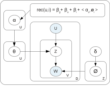
Figure IV.2: Supervised model for user facets and ratings.

An elegant approach using Multinomial-Dirichlet Regression is proposed in [Mimno 2008] to incorporate arbitrary types of observed continuous or categorical features. Each facet $z$ is associated with a vector $\lambda_{z}$ whose dimension equals the number of features. Assuming $x_{d}$ is the feature vector for document $d$, the Dirichlet hyper-parameter $\alpha$ for the document-facet Multinomial distribution $\Theta$ is parametrized as $\alpha_{d,z}=exp(x_{d}^{T}\lambda_{z})$. The model is trained using stochastic EM which alternates between 1) sampling facet assignments from the posterior distribution conditioned on words and features, and 2) optimizing $\lambda$ given the facet assignments using L-BFGS. Our approach, explained in the next section, follows a similar approach to couple the User-Facet Model and the Latent-Factor Recommendation Model (depicted in Figure IV.2).

IV.3.4 Joint Model: User Experience, Facet Preference, Writing Style

Figure IV.3: Supervised model for user experience, facets, and ratings.

We start with a User-Facet Model (UFM) (aka. Author-Topic Model [Rosen-Zvi 2004b]) based on Latent Dirichlet Allocation (LDA), where users have a distribution over facets and facets have a distribution over words. This is to determine the facets of interest to a user. These facet preferences can be interpreted as latent item factors in the traditional Latent-Factor Recommendation Model (LFM) [Koren 2008]. However, the LFM is supervised as opposed to the UFM. It is not obvious how to incorporate supervision into the UFM to predict ratings. The user-provided ratings of items can take continuous values (in some review communities), so we cannot incorporate them into a UFM with a Multinomial distribution of ratings. We propose an Expectation-Maximization (EM) approach to incorporate supervision, where the latent facets are estimated in an E-Step using Gibbs Sampling, and Support Vector Regression (SVR) [Drucker 1996] is used in the M-Step to learn the feature weights and predict ratings. Subsequently, we incorporate a layer for experience in the UFM-LFM model, where the experience levels are drawn from a Hidden Markov Model (HMM) in the E-Step. The experience level transitions depend on the evolution of the user’s maturing rate, facet preferences, and writing style over time. The entire process is a supervised generative process of generating a review based on the experience level of a user hinged on our HMM-LDA model.

Generative Process for a Review

Consider a corpus with a set $D$ of review documents denoted by $\{d_{1}\dots d_{D}\}$. For each user, all her documents are ordered by timestamps $t$ when she wrote them, such that $t_{d_{i}}<t_{d_{j}}$ for $i<j$. Each document $d$ has a sequence of $N_{d}$ words denoted by $d=\{w_{1}\dots.w_{N_{d}}\}$. Each word is drawn from a vocabulary $V$ having unique words indexed by $\{1\dots V\}$. Consider a set of $U$ users involved in writing the documents in the corpus, where $u_{d}$ is the author of document $d$. Consider an ordered set of experience levels $\{e_{1},e_{2},...e_{E}\}$ where each $e_{i}$ is from a set $E$, and a set of facets $\{z_{1},z_{2},...z_{Z}\}$ where each $z_{i}$ is from a set $Z$ of possible facets. Each document $d$ is associated with a rating $r$ and an item $i$.

At the time $t_{d}$ of writing the review $d$, the user $u_{d}$ has experience level $e_{t_{d}}\in E$. We assume that her experience level transitions follow a distribution $\Pi$ with a Markovian assumption and certain constraints. This means the experience level of $u_{d}$ at time $t_{d}$ depends on her experience level when writing the previous document at time $t_{d-1}$.

$\pi_{e_{i}}(e_{j})$ denotes the probability of progressing to experience level $e_{j}$ from experience level $e_{i}$, with the constraint $e_{j}\in\{e_{i},e_{i}+1\}$. This means at each instant the user can either stay at her current experience level, or move to the next one.

The experience-level transition probabilities depend on the rating behavior, facet preferences, and writing style of the user. The progression also takes into account the 1) maturing rate of $u_{d}$ modeled by the intensity of her activity in the community, and 2) the time interval between writing consecutive reviews. We incorporate these aspects in a prior for the user’s transition rates, $\gamma^{u_{d}}$, defined as:

$$\gamma^{u_{d}}=\frac{D_{u_{d}}}{D_{u_{d}}+D_{avg}}+{\lambda(t_{d}-t_{d-1})}$$

$D_{u_{d}}$ and $D_{avg}$ denote the number of reviews written by ${u_{d}}$ and the average number of reviews per user in the community, respectively. Therefore the first term models the user activity with respect to the community average. The second term reflects the time interval between successive reviews. The user experience is unlikely to change from the level when writing the previous review just a few hours or days ago. $\lambda$ controls the effect of this time difference, and is set to a very small value. Note that if the user writes very infrequently, the second term may go up. But the first term which plays the dominating role in this prior will be very small with respect to the community average in an active community, bringing down the influence of the entire prior. Note that the constructed HMM encapsulates all the factors for experience progression outlined in Section IV.3.1.

At experience level $e_{t_{d}}$, user $u_{d}$ has a Multinomial facet-preference distribution $\theta_{u_{d},e_{t_{d}}}$. From this distribution she draws a facet of interest $z_{d_{i}}$ for the $i^{th}$ word in her document. For example, a user at a high level of experience may choose to write on the beer “hoppiness” or “story perplexity” in a movie. The word that she writes depends on the facet chosen and the language model for her current experience level. Thus, she draws a word from the multinomial distribution $\phi_{e_{t_{d}},z_{d_{i}}}$ with a symmetric Dirichlet prior $\delta$. For example, if the facet chosen is beer taste or movie plot, an experienced user may choose to use the words “coffee roasted vanilla” and “visceral”, whereas an inexperienced user may use “bitter” and “emotional” respectively.

Algorithm 4 describes this generative process for the review; Figure IV.8 depicts it visually in plate notation for graphical models. We use MCMC sampling for inference on this model.

for each facet $z=1,...Z$ and experience level $e=1,...E$ do

      choose $\phi_{e,z}\sim Dirichlet(\beta)$

end for

for each review $d=1,...D$ do

       Given user $u_{d}$ and timestamp $t_{d}$

       /*Current experience level depends on previous level*/

       1. Conditioned on $u_{d}$ and previous experience $e_{t_{d-1}}$, choose $e_{t_{d}}\sim\pi_{e_{t_{d-1}}}$

       /*User’s facet preferences at current experience level are influenced by supervision via $\alpha$    –    scaled by hyper-parameter $\rho$ controlling influence of supervision*/

       2. Conditioned on supervised facet preference $\alpha_{u_{d},e_{t_{d}}}$ of $u_{d}$ at experience level $e_{t_{d}}$ scaled by $\rho$, choose $\theta_{u_{d},e_{t_{d}}}\sim Dirichlet(\rho\times\alpha_{u_{d},e_{t_{d}}})$

       for each word $i=1,...N_{d}$ do

             /*Facet is drawn from user’s experience-based facet interests*/

             3. Conditioned on $u_{d}$ and $e_{t_{d}}$ choose a facet $z_{d_{i}}\sim Multinomial(\theta_{u_{d},e_{t_{d}}})$

             /*Word is drawn from chosen facet and user’s vocabulary at her current experience level*/

             4. Conditioned on $z_{d_{i}}$ and $e_{t_{d}}$ choose a word $w_{d_{i}}\sim Multinomial(\phi_{e_{t_{d}},z_{d_{i}}})$

            

       end for

      /*Rating computed via Support Vector Regression with

       chosen facet proportions as input features to learn $\alpha$*/

       5. Choose $r_{d}\sim F(\langle{\alpha_{u_{d},e_{t_{d}}}},\phi_{e_{t_{d}},z_{d}}\rangle)$

      

end for

Algorithm 2 Supervised Generative Model for a User’s Experience, Facets, and Ratings

Supervision for Rating Prediction

The latent item factors $\phi_{i}$ in Equation IV.2 correspond to the latent facets $Z$ in Algorithm 4. Assume that we have some estimation of the latent facet distribution $\phi_{e,z}$ of each document after one iteration of MCMC sampling, where $e$ denotes the experience level at which a document is written, and let $z$ denote a latent facet of the document. We also have an estimation of the preference of a user $u$ for facet $z$ at experience level $e$ given by $\theta_{u,e}(z)$.

For each user $u$, we compute a supervised regression function $F_{u}$ for the user’s numeric ratings with the – currently estimated – experience-based facet distribution $\phi_{e,z}$ of her reviews as input features and the ratings as output.

The learned feature weights $\langle\alpha_{u,e}(z)\rangle$ indicate the user’s preference for facet $z$ at experience level $e$. These feature weights are used to modify $\theta_{u,e}$ to attribute more mass to the facet for which $u$ has a higher preference at level $e$. This is reflected in the next sampling iteration, when we draw a facet $z$ from the user’s facet preference distribution $\theta_{u,e}$ smoothed by $\alpha_{u,e}$, and then draw a word from $\phi_{e,z}$. This sampling process is repeated until convergence.

In any latent facet model, it is difficult to set the hyper-parameters. Therefore, most prior work assume symmetric Dirichlet priors with heuristically chosen concentration parameters. Our approach is to learn the concentration parameter $\alpha$ of a general (i.e., asymmetric) Dirichlet prior for Multinomial distribution $\Theta$ – where we optimize these hyper-parameters to learn user ratings for documents at a given experience level.

Inference

We describe the inference algorithm to estimate the distributions $\Theta$, $\Phi$ and $\Pi$ from observed data. For each user, we compute the conditional distribution over the set of hidden variables $E$ and $Z$ for all the words $W$ in a review. The exact computation of this distribution is intractable. We use Collapsed Gibbs Sampling [Griffiths 2002] to estimate the conditional distribution for each hidden variable, which is computed over the current assignment for all other hidden variables, and integrating out other parameters of the model.

Let $U,E,Z$ and $W$ be the set of all users, experience levels, facets and words in the corpus. In the following, $i$ indexes a document and $j$ indexes a word in it.

The joint probability distribution is given by:

$$P(U,E,Z,W,\theta,\phi,\pi;\alpha,\delta,\gamma)=\prod_{u=1}^{U}\prod_{e=1}^{E}\prod_{i=1}^{D_{u}}\prod_{z=1}^{Z}\prod_{j=1}^{{N_{d_{u}}}}\\ \{\underbrace{P(\pi_{e};\gamma^{u})\times P(e_{i}|\pi_{e})}_{\text{experience transition distribution}}\times\underbrace{P(\theta_{u,e};\alpha_{u,e})\times P(z_{i,j}|\theta_{u,e_{i}})}_{\text{user experience facet distribution}}\times\underbrace{P(\phi_{e,z};\delta)\times P(w_{i,j}|\phi_{e_{i},z_{i,j}})}_{\text{experience facet language distribution}}\}$$ (IV.3)

Let $n(u,e,d,z,v)$ denote the count of the word $w$ occurring in document $d$ written by user $u$ at experience level $e$ belonging to facet $z$. In the following equation, $(.)$ at any position in a distribution indicates summation of the above counts for the respective argument.

Exploiting conjugacy of the Multinomial and Dirichlet distributions, we can integrate out $\Phi$ from the above distribution to obtain the posterior distribution $P(Z|U,E;\alpha)$ of the latent variable $Z$ given by:

$$\prod_{u=1}^{U}\prod_{e=1}^{E}\frac{\Gamma(\sum_{z}\alpha_{u,e,z})\prod_{z}\Gamma(n(u,e,.,z,.)+\alpha_{u,e,z})}{\prod_{z}{\Gamma(\alpha_{u,e,z})\Gamma(\sum_{z}n(u,e,.,z,.)+\sum_{z}\alpha_{u,e,z})}}$$

         where $\Gamma$ denotes the Gamma function.

Similarly, by integrating out $\Theta$, $P(W|E,Z;\delta)$ is given by

$$\prod_{e=1}^{E}\prod_{z=1}^{Z}\frac{\Gamma(\sum_{v}\delta_{v})\prod_{v}\Gamma(n(.,e,.,z,v)+\delta_{v})}{\prod_{v}{\Gamma(\delta_{v})\Gamma(\sum_{v}n(.,e,.,z,v)+\sum_{v}\delta_{v})}}$$

Let $m_{e_{i}}^{e_{i-1}}$ denote the number of transitions from experience level $e_{i-1}$ to $e_{i}$ over all users in the community, with the constraint $e_{i}\in\{e_{i-1},e_{i-1}+1\}$. Note that we allow self-transitions for staying at the same experience level. The counts capture the relative difficulty in progressing between different experience levels. For example, it may be easier to progress to level $2$ from level $1$ than to level $4$ from level $3$.

The state transition probability depending on the previous state, factoring in the user-specific activity rate, is given by:

$\hskip 30.00005ptP(e_{i}|e_{i-1},u,e_{-i})=\frac{m_{e_{i}}^{e_{i-1}}+I(e_{i-1}=e_{i})+\gamma^{u}}{m_{.}^{e_{i-1}}+I(e_{i-1}=e_{i})+E\gamma^{u}}$

where $I(.)$ is an indicator function taking the value $1$ when the argument is true, and $0$ otherwise. The subscript $-i$ denotes the value of a variable excluding the data at the $i^{th}$ position. All the counts of transitions exclude transitions to and from $e_{i}$, when sampling a value for the current experience level $e_{i}$ during Gibbs sampling. The conditional distribution for the experience level transition is given by:

$$P(E|U,Z,W)\propto P(E|U)\times P(Z|E,U)\times P(W|Z,E)$$ (IV.4)

Here the first factor models the rate of experience progression factoring in user activity; the second and third factor models the facet-preferences of user, and language model at a specific level of experience respectively. All three factors combined decide whether the user should stay at the current level of experience, or has matured enough to progress to next level.

In Gibbs sampling, the conditional distribution for each hidden variable is computed based on the current assignment of other hidden variables. The values for the latent variables are sampled repeatedly from this conditional distribution until convergence. In our problem setting we have two sets of latent variables corresponding to $E$ and $Z$ respectively.

We perform Collapsed Gibbs Sampling [Griffiths 2002] in which we first sample a value for the experience level $e_{i}$ of the user for the current document $i$, keeping all facet assignments $Z$ fixed. In order to do this, we consider two experience levels $e_{i-1}$ and ${e_{i-1}+1}$. For each of these levels, we go through the current document and all the token positions to compute Equation IV.4 — and choose the level having the highest conditional probability. Thereafter, we sample a new facet for each word $w_{i,j}$ of the document, keeping the currently sampled experience level of the user for the document fixed.

The conditional distributions for Gibbs sampling for the joint update of the latent variables $E$ and $Z$ are given by:

$$\textbf{E-Step 1: }P(e_{i}=e|e_{i-1},u_{i}=u,\{z_{i,j}=z_{j}\},\{w_{i,j}=w_{j}\},e_{-i})\propto\\ P(e_{i}|u,e_{i-1},e_{-i})\times\prod_{j}P(z_{j}|e_{i},u,e_{-i})\times P(w_{j}|z_{j},e_{i},e_{-i})\propto\\ \frac{m_{e_{i}}^{e_{i-1}}+I(e_{i-1}=e_{i})+\gamma^{u}}{m_{.}^{e_{i-1}}+I(e_{i-1}=e_{i})+E\gamma^{u}}\times\prod_{j}\frac{n(u,e,.,z_{j},.)+\alpha_{u,e,z_{j}}}{\sum_{z_{j}}n(u,e,.,z_{j},.)+\sum_{z_{j}}\alpha_{u,e,z_{j}}}\times\frac{n(.,e,.,z_{j},w_{j})+\delta}{\sum_{w_{j}}n(.,e,.,z_{j},w_{j})+V\delta}\\ \\ \noindent\textbf{E-Step 2:\quad\quad}P(z_{j}=z|u_{d}=u,e_{d}=e,w_{j}=w,z_{-j})\propto\\ \frac{n(u,e,.,z,.)+\alpha_{u,e,z}}{\sum_{z}n(u,e,.,z,.)+\sum_{z}\alpha_{u,e,z}}\times\frac{n(.,e,.,z,w)+\delta}{\sum_{w}n(.,e,.,z,w)+V\delta}\\$$ (IV.5)

The proportion of the $z^{th}$ facet in document $d$ with words $\{w_{j}\}$ written at experience level $e$ is given by:

$$\centering\phi_{e,z}(d)=\frac{\sum_{j=1}^{N_{d}}\phi_{e,z}(w_{j})}{N_{d}}\@add@centering$$

For each user $u$, we learn a regression model $F_{u}$ using these facet proportions in each document as features, along with the user and item biases (refer to Equation IV.2), with the user’s item rating $r_{d}$ as the response variable. Besides the facet distribution of each document, the biases $<\beta_{g}(e),\beta_{u}(e),\beta_{i}(e)>$ also depend on the experience level $e$.

We formulate the function $F_{u}$ as Support Vector Regression [Drucker 1996], which forms the $M$-$Step$ in our problem:

$$\textbf{M-Step: }\min_{\alpha_{u,e}}\frac{1}{2}{\alpha_{u,e}} {}^{T}{\alpha_{u,e}}+C\times\sum_{d=1}^{D_{u}}(max(0,|r_{d}-{\alpha_{u,e}}^{T}<\beta_{g}(e), \beta_{u}(e),\beta_{i}(e),\phi_{e,z}(d)>|-\epsilon))^{2}$$

The total number of parameters learned is $[E\times Z+E\times 3]\times U$. Our solution may generate a mix of positive and negative real numbered weights. In order to ensure that the concentration parameters of the Dirichlet distribution are positive reals, we take $exp(\alpha_{u,e})$. The learned $\alpha$’s are typically very small, whereas the value of $n(u,e,.,z,.)$ in Equation IV.5 is very large. Therefore we scale the $\alpha$’s by a hyper-parameter $\rho$ to control the influence of supervision. $\rho$ is tuned using a validation set by varying it from $\{10^{0},10^{1}...10^{5}\}$. In the E-Step of the next iteration, we choose $\theta_{u,e}\sim Dirichlet(\rho\times\alpha_{u,e})$. We use the LibLinear package for Support Vector Regression.

IV.3.5 Experiments

Setup: Data and Baselines

Data: We perform experiments with data from five communities in different domains:
BeerAdvocate (beeradvocate.com) and RateBeer (ratebeer.com) for beer reviews, Amazon (amazon.com) for movie reviews, Yelp (yelp.com) for food and restaurant reviews, and
NewsTrust (newstrust.net) for reviews of news media. Table IV.3 gives the dataset statistics. We have a total of $12.7$ million reviews from $0.9$ million users from all of the five communities combined. The first four communities are used for product reviews, from where we extract the following quintuple for our model $<userId,itemId,timestamp,rating,review>$.
NewsTrust is a special community, which we discuss in Section IV.5.

For all models, we used the three most recent reviews of each user as withheld test data. All experience-based models consider the last experience level reached by each user, and corresponding learned parameters for rating prediction. In all the models, we group light users with less than $50$ reviews in training data into a background model, treated as a single user, to avoid modeling from sparse observations. We do not ignore any user. During the test phase for a light user, we take her parameters from the background model. We set $Z=20$ for BeerAdvocate, RateBeer and Yelp facets; and $Z=100$ for Amazon movies and NewsTrust which have much richer latent dimensions. For experience levels, we set $E=5$ for all. However, for NewsTrust and Yelp datasets our model categorizes users to belong to one of three experience levels.

Dataset	#Users	#Items	#Ratings
Beer (BeerAdvocate)	33,387	66,051	1,586,259
Beer (RateBeer)	40,213	110,419	2,924,127
Movies (Amazon)	759,899	267,320	7,911,684
Food (Yelp)	45,981	11,537	229,907
Media (NewsTrust)	6,180	62,108	134,407
TOTAL	885,660	517,435	12,786,384

Table IV.3: Dataset statistics.

Baselines: We consider the following baselines for our work, and use the available code for experimentation.

• LFM: A standard latent factor recommendation model [Koren 2008].

• Community at uniform rate: Users and products in a community evolve using a single “global clock” [Koren 2010][Xiong 2010][Xiang 2010], where the different stages of the community evolution appear at uniform time intervals. So the community prefers different products at different times.

• Community at learned rate: This extends (b) by learning the rate at which the community evolves with time, eliminating the uniform rate assumption.

• User at uniform rate: This extends (b) to consider individual users, by modeling the different stages of a user’s progression based on preferences and experience levels evolving over time. The model assumes a uniform rate for experience progression.

• User at learned rate: This extends (d) by allowing each user to evolve on a “personal clock”, so that the time to reach certain experience levels depends on the user
  [McAuley 2013b].

f) Our model with past experience level: In order to determine how well our model captures evolution of user experience over time, we consider another baseline where we randomly sample the experience level reached by users at some timepoint previously in their lifecycle, who may have evolved thereafter. We learn our model parameters from the data up to this time, and again predict the user’s most recent three item ratings. Note that this baseline considers textual content of user contributed reviews, unlike other baselines that ignore them. Therefore it is better than vanilla content-based methods, with the notion of past evolution, and is the strongest baseline for our model.

Quantitative Comparison

Models	Beer	Rate	News	Amazon	Yelp
	Advocate	Beer	Trust
Our model	0.363	0.309	0.373	1.174	1.469
(most recent experience level)
f) Our model	0.375	0.362	0.470	1.200	1.642
(past experience level)
e) User at learned rate	0.379	0.336	0.575	1.293	1.732
c) Community at learned rate	0.383	0.334	0.656	1.203	1.534
b) Community at uniform rate	0.391	0.347	0.767	1.203	1.526
d) User at uniform rate	0.394	0.349	0.744	1.206	1.613
a) Latent factor model	0.409	0.377	0.847	1.248	1.560

Table IV.4: MSE comparison of our model versus baselines.

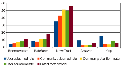
Figure IV.4: MSE improvement (%) of our model over baselines.

Discussions: Table IV.4 compares the mean squared error (MSE) for rating predictions, generated by our model versus the six baselines. Our model consistently outperforms all baselines, reducing the MSE by ca. $5$ to $35\%$. Improvements of our model over baselines are statistically significant at p-value $<0.0001$.

Our performance improvement is most prominent for the NewsTrust community, which exhibits strong language features, and topic polarities in reviews. The lowest improvement (over the best performing baseline in any dataset) is achieved for Amazon movie reviews. A possible reason is that the community is very diverse with a very wide range of movies and that review texts heavily mix statements about movie plots with the actual review aspects like praising or criticizing certain facets of a movie. The situation is similar for the food and restaurants case. Nevertheless, our model always wins over the best baseline from other works, which is typically the “user at learned rate" model.

Evolution effects: We observe in Table IV.4 that our model’s predictions degrade when applied to the users’ past experience level, compared to their most recent level. This signals that the model captures user evolution past the previous timepoint. Therefore the last (i.e., most recent) experience level attained by a user is most informative for generating new recommendations.

Experience Level 1: drank, bad, maybe, terrible, dull, shit
Experience Level 2: bottle, sweet, nice hops, bitter, strong light, head, smooth, good, brew, better, good
Expertise Level 3: sweet alcohol, palate down, thin glass, malts, poured thick, pleasant hint, bitterness, copper hard
Experience Level 4: smells sweet, thin bitter, fresh hint, honey end, sticky yellow, slight bit good, faint bitter beer, red brown, good malty, deep smooth bubbly, damn weak
Experience Level 5: golden head lacing, floral dark fruits, citrus sweet, light spice, hops, caramel finish, acquired taste, hazy body, lacing chocolate, coffee roasted vanilla, creamy bitterness, copper malts, spicy honey

Table IV.5: Experience-based facet words for the illustrative beer facet taste.

Qualitative Analysis

Salient words for facets and experience levels: We point out typical word clusters, with illustrative labels, to show the variation of language for users of different experience levels and different facets. Tables IV.2 and IV.5 show salient words to describe the beer facet taste and movie facets plot and narrative style, respectively – at different experience levels. Note that the facets being latent, their labels are merely our interpretation. Other similar examples can be found in Tables IV.1 and IV.10.

BeerAdvocate and RateBeer are very focused communities; so it is easier for our model to characterize the user experience evolution by vocabulary and writing style in user reviews. We observe in Table IV.5 that users write more descriptive and fruity words to depict the beer taste as they become more experienced.

For movies, the wording in reviews is much more diverse and harder to track. Especially for blockbuster movies, which tend to dominate this data, the reviews mix all kinds of aspects. A better approach here could be to focus on specific kinds of movies (e.g., by genre or production studios) that may better distinguish experienced users from amateurs or novices in terms of their refined taste and writing style.

MSE for different experience levels: We observe a weak trend that the MSE decreases with increasing experience level. Users at the highest level of experience almost always exhibit the lowest MSE, and, therefore, more preditable in their behavior. So we tend to better predict the rating behavior for the most mature users than for the remaining user population. This in turn enables generating better recommendations for the “connoisseurs" in the community.

Experience progression: Figure IV.5 shows the proportion of reviews written by community members at different experience levels right before advancing to the next level. Here we plot users with a minimum of $50$ reviews, so they are certainly not “amateurs". A large part of the community progresses from level $1$ to level $2$. However, from here only few users move to higher levels, leading to a skewed distribution. We observe that the majority of the population stays at level $2$.

Figure IV.5: Proportion of reviews at each experience level of users.

Datasets	e=1	e=2	e=3	e=4	e=5
BeerAdvocate	0.05	0.59	0.19	0.10	0.07
RateBeer	0.03	0.42	0.35	0.18	0.02
NewsTrust	-	-	0.15	0.60	0.25
Amazon	-	0.72	0.13	0.10	0.05
Yelp	-	-	0.30	0.68	0.02

Table IV.6: Distribution of users at different experience levels.

User experience distribution: Table IV.6 shows the number of users per experience level in each domain, for users with $>50$ reviews. The distribution also follows our intuition of a highly skewed distribution. Note that almost all users with $<50$ reviews belong to levels 1 or 2.

Language model and facet preference divergence: Figure IV.6(b) and IV.6(c) show the $KL$ divergence for facet-preference and language models of users at different experience levels, as computed by our model. The facet-preference divergence increases with the gap between experience levels, but not as smooth and prominent as for the language models. On one hand, this is due to the complexity of latent facets vs. explicit words. On the other hand, this also affirms our notion of grounding the model on language.

Baseline model divergence: Figure IV.6(a) shows the facet-preference divergence of users at different experience levels computed by the baseline model “user at learned rate” [McAuley 2013b]. The contrast between the heatmaps of our model and the baseline is revealing. The increase in divergence with increasing gap between experience levels is very rough in the baseline model, although the trend is obvious.

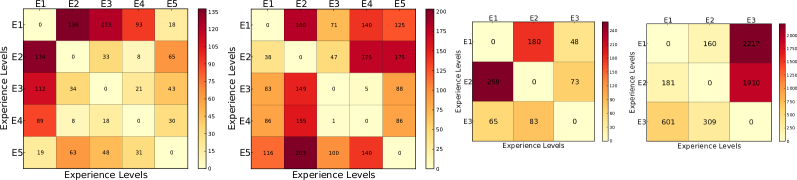
(a) User at learned rate [McAuley 2013b]: Facet preference divergence with experience.

(b) Our model: Facet preference divergence with experience.

(c) Our model: Language model divergence with experience.

Figure IV.6: Facet preference and language model $KL$ divergence with experience.

IV.4 Continuous Experience Evolution

In the previous section, we presented an approach to model the experience evolution of users in online communities. However, the proposed model has several assumptions, and resulting drawbacks. In the following, we propose a generalized model that captures the evolution of user experience as is commonly observed in the Nature.

IV.4.1 Model Components

Importance of Time

Previous approaches [Section IV.3] [McAuley 2013b] on experience evolution model time only implicitly by assuming the (discrete) latent experience to progress from one review to the next. In contrast, we now model time explicitly, and allow experience to continuously evolve over time — so that we are able to trace the joint evolution of experience, and vocabulary. This is challenging as the discrete Multinomial distribution based language model (to generate words) needs to be combined with a continuous stochastic process for experience evolution.

We use two levels of temporal granularity. Since experience is naturally continuous, it is beneficial to model its evolution at a very fine resolution (say, minutes or hours). On the other hand, the language model has a much coarser granularity (say, days, weeks or months). We show in Section IV.4.2 how to smoothly merge the two granularities using continuous-time models. Our model for language evolution is motivated by the seminal work of Wang and Blei et al. [Wang 2012], with major differences and extensions. In the following subsections, we formally introduce the two components affected by time: the experience evolution and the language model evolution.

Continuous Experience Evolution

Prior approaches [Section IV.3] [McAuley 2013b] model experience as a discrete random variable . At each timepoint, a user is allowed to stay at level $l$, or move to level $l+1$. As a result the transition is abrupt when the user switches levels. Also, the model does not distinguish between users at the same level of experience, (or even for the same user at beginning or end of a level) even though their experience can be quite far apart (if measured in a continuous scale). For instance, in Figure IV.7(b) the language model uses the same set of parameters as long as the user stays at level $1$, although the language model changes.

(a) Evolution of an experienced user.

(b) Evolution of an amateur user.

Figure IV.7: Discrete state and continuous state experience evolution of some typical users from the BeerAdvocate community.

In order to address these issues, our goal is to develop a continuous experience evolution model with the following requirements:

• The experience value is always positive.

• Markovian assumption for the continuous-time process: The experience value at any time $t$ depends only on the value at the most recent observed time prior to $t$.

• Drift: It has an overall trend to increase over time.

• Volatility: The evolution may not be smooth with occasional volatility. For instance, an experienced user may write a series of expert reviews, followed by a sloppy one.

To capture all of these aspects, we model each user’s experience as a Geometric Brownian Motion (GBM) process (also known as Exponential Brownian Motion).

GBM is a natural continuous state alternative to the discrete-state space based Hidden Markov Model (HMM) used in our previous approach (refer to Section IV.3). Figure IV.7 shows a real-world example of the evolution of an experienced and amateur user in the BeerAdvocate community, as traced by our proposed model — along with that of its discrete counterpart from our previous approach. The GBM is a stochastic process used to model population growth, financial processes like stock price behavior (e.g., Black-Scholes model) with random noise. It is a continuous time stochastic process, where the logarithm of the random variable (say, $X_{t}$) follows Brownian Motion with a volatility and drift. Formally, a stochastic process $X_{t}$, with an arbitrary initial value $X_{0}$, for $t\in[0,\infty)$ is said to follow Geometric Brownian Motion, if it satisfies the following Stochastic Differential Equation (SDE) [Karatzas 1991]:

$$dX_{t}=\mu X_{t}dt+\sigma X_{t}dW_{t}$$ (IV.6)

where, $W_{t}$ is a Wiener process (Standard Brownian Motion); $\mu\in\mathbb{R}$ and $\sigma\in(0,\infty)$ are constants called the percentage trend and percentage volatility respectively. The former captures deterministic trends, whereas the latter captures unpredictable events occurring during the motion.

In a Brownian Motion trajectory, $\mu X_{t}dt$ and $\sigma X_{t}dW_{t}$ capture the “trend” and “volatility”, as is required for experience evolution. However, in real life communities each user might show a different experience evolution; therefore our model considers a multivariate version of this GBM – we model one trajectory per-user. Correspondingly, during the inference process we learn $\mu_{u}$ and $\sigma_{u}$ for each user $u$.

Properties: A straightforward application of Itô’s formula yields the following analytic solution to the above SDE (Equation IV.6):

$$X_{t} =X_{0}\ exp\big{(}(\mu-\frac{\sigma^{2}}{2})t+\sigma W_{t}\big{)}$$ (IV.7)

Since $log(X_{t})$ follows a Normal distribution, $X_{t}$ is Log-Normally distributed with mean $\big{(}log(X_{0})+(\mu-\frac{\sigma^{2}}{2})t\big{)}$ and variance $\sigma\sqrt{t}$. The probability density function $f_{t}(x)$, for $x\in(0,\infty)$, is given by:

$$f_{t}(x)=\frac{1}{\sqrt{2\pi t}\sigma x}exp\bigg{(}-\frac{\big{(}log(x)-log\ (x_{0})-(\mu-\frac{\sigma^{2}}{2})t\big{)}^{2}}{2\sigma^{2}t}\bigg{)}$$ (IV.8)

It is easy to show that GBM has the Markov property. Consider $U_{t}=(\mu-\frac{\sigma^{2}}{2})t+\sigma W_{t}$.

$$X_{t+h} =X_{0}exp(U_{t+h})$$ (IV.9)

$$=X_{0}exp(U_{t}+U_{t+h}-U_{t})$$

$$=X_{0}exp(U_{t})exp(U_{t+h}-U_{t})$$

$$=X_{t}exp(U_{t+h}-U_{t})$$

Therefore, future states depend only on the future increment of the Brownian Motion, which satisfies our requirement for experience evolution. Also, for $X_{0}>0$, the GBM process is always positive. Note that the start time of the GBM of each user is relative to her first review in the community.

Experience-aware Language Evolution

Once the experience values for each user are generated from a Log-Normal distribution (more precisely: the experience of the user at the times when she wrote each review), we develop the language model whose parameters evolve according to the Markov property for experience evolution.

As users get more experienced, they use more sophisticated words to express a concept. For instance, experienced cineastes refer to a movie’s “protagonist” whereas amateur movie lovers talk about the “hero”. Similarly, in a Beer review community (e.g., BeerAdvocate, RateBeer) experts use more fruity words to describe a beer like “caramel finish, coffee roasted vanilla”, and “citrus hops”. Facet preferences of users also evolve with experience. For example, users at a high level of experience prefer “hoppiest” beers which are considered too “bitter” by amateurs [McAuley 2013b]. Encoding explicit time in our model allows us to trace the evolution of vocabulary and trends jointly on the temporal and experience dimension.

Latent Dirichlet Allocation (LDA): In the traditional LDA process [Blei 2001], a document is assumed to have a distribution over $Z$ facets (a.k.a. topics) $\beta_{1:Z}$, and each of the facets has a distribution over words from a fixed vocabulary collection. The per-facet word (a.k.a topic-word) distribution $\beta_{z}$ is drawn from a Dirichlet distribution, and words $w$ are generated from a Multinomial($\beta_{z}$).

The process assumes that documents are drawn exchangeably from the same set of facets. However, this process neither takes experience nor the evolution of the facets over time into account.

Discrete Experience-aware LDA: Our previous approach (refer to Section IV.3) incorporates a layer for experience in the above process. The user experience is manifested in the set of facets that the user chooses to write on, and the vocabulary and writing style used in the reviews. The experience levels were drawn from a Hidden Markov Model (HMM). The reviews were assumed to be exchangeable for a user at the same level of experience – an assumption which generally may not hold; since the language model of a user at the same discrete experience level may be different at different points in time (refer to Figure IV.7(b)) (if we had a continuous scale for measuring experience). The process considers time only implicitly via the transition of the latent variable for experience.

Continuous Time LDA: The seminal work of [Blei 2006, Wang 2012] capture evolving content, for instance, in scholarly journals and news articles where the themes evolve over time, by considering time explicitly in the generative LDA process. Our language model evolution is motivated by their Continuous Time Dynamic Topic Model [Blei 2006], with the major difference that the facets, in our case, evolve over both time and experience.

Continuous Experience-aware LDA (this work): Since the assumption of exchangeability of documents at the same level of experience of a user may not hold, we want the language model to explicitly evolve over experience and time. To incorporate the effect of changing experience levels, our goal is to condition the parameter evolution of $\beta$ on the experience progression.

In more detail, for the language model evolution, we desire the following properties:

• It should smoothly evolve over time preserving the Markov property of experience evolution.

• Its variance should linearly increase with the experience change between successive timepoints. This entails that if the experience of a user does not change between successive timepoints, the language model remains almost the same.

To incorporate the temporal aspects of data, in our model, we use multiple distributions $\beta_{t,z}$ for each time $t$ and facet $z$. Furthermore, to capture the smooth temporal evolution of the facet language model, we need to chain the different distributions to sequentially evolve over time $t$: the distribution $\beta_{t,z}$ should affect the distribution $\beta_{t+1,z}$.

Since the traditional parametrization of a Multinomial distribution via its mean parameters is not amenable to sequential modeling, and inconvenient to work with in gradient based optimization – since any gradient step requires the projection to the feasible set, the simplex — we follow a similar approach as [Wang 2012]: instead of operating on the mean parameters, we consider the natural parameters of the Multinomial. The natural parameters are unconstrained and, thus, enable an easier sequential modeling.

From now on, we denote with $\beta_{t,z}$ the natural parameters of the Multinomial at time $t$ for facet $z$. For identifiability one of the parameters $\beta_{t,z,w}$ needs to be fixed at zero. By applying the following mapping we can obtain back the mean parameters that are located on the simplex:

$$\pi(\beta_{t,z,w})=\frac{exp(\beta_{t,z,w})}{1+\sum_{w=1}^{V-1}exp(\beta_{t,z,w})}$$ (IV.10)

Using the natural parameters, we can now define the facet-model evolution: The underlying idea is that strong changes in the users’ experience can lead to strong changes in the language model, while low changes should lead to only few changes. To capture this effect, let $l_{t,w}$ denote the average experience of a word $w$ at time $t$ (e.g. the value of $l_{t,w}$ is high if many experienced users have used the word). That is, $l_{t,w}$ is given by the average experience of all the reviews $D_{t}$ containing the word $w$ at time $t$.

$$l_{t,w}=\frac{\sum_{d\in D_{t}:w\in d}e_{d}}{|D_{t}|}$$ (IV.11)

where, $e_{d}$ is the experience value of review $d$ (i.e. the experience of user $u_{d}$ at the time of writing the review).

The language model evolution is then modeled as:

$$\beta_{t,z,w}\sim Normal(\beta_{t-1,z,w},\sigma\cdot|l_{t,w}-l_{t-1,w}|)$$ (IV.12)

Here, we simply follow the idea of a standard dynamic system with Gaussian noise, where the mean is the value at the previous timepoint, and the variance increases linearly with increasing change in the experience. Thereby, the desired properties of the language model evolution are ensured.

IV.4.2 Joint Model for Experience-Language Evolution

Generative Process

Consider a corpus $D=\{d_{1},\ldots,d_{D}\}$ of review documents written by a set of users $U$ at timestamps $T$. For each review $d\in D$, we denote $u_{d}$ as its user, $t^{\prime}_{d}$ as the fine-grained timestamp of the review (e.g. minutes or seconds; used for experience evolution) and with $t_{d}$ the timestamp of coarser granularity (e.g. yearly or monthly; used for language model evolution). The reviews are assumed to be ordered by timestamps, i.e. $t{{}^{\prime}}_{d_{i}}<t{{}^{\prime}}_{d_{j}}$ for $i<j$. We denote with $D_{t}=\{d\in D\mid t_{d}=t\}$ all reviews written at timepoint $t$. Each review $d\in D$ consists of a sequence of $N_{d}$ words denoted by $d=\{w_{1},\ldots,w_{N_{d}}\}$, where each word is drawn from a vocabulary $V$ having unique words indexed by $\{1\dots V\}$. The number of facets corresponds to $Z$.

Let $e_{d}\in(0,\infty)$ denote the experience value of review $d$. Since each review $d$ is associated with a unique timestamp $t^{\prime}_{d}$ and unique user $u_{d}$, the experience value of a review refers to the experience of the user at the time of writing it. In our model, each user $u$ follows her own Geometric Brownian Motion trajectory – starting time of which is relative to the first review of the user in the community – parametrized by the mean $\mu_{u}$, variance $\sigma_{u}$, and her starting experience value $s_{0,u}$. As shown in Equation IV.8, the analytical form of a GBM translates to a Log-Normal distribution with the given mean and variance. We use this user-dependent distribution to generate an experience value $e_{d}$ for the review $d$ written by her at timestamp $t^{\prime}_{d}$.

Following standard LDA, the facet proportion $\theta_{d}$ of the review is drawn from a Dirichlet distribution with concentration parameter $\alpha$, and the facet $z_{d,w}$ of each word $w$ in $d$ is drawn from a Multinomial($\theta_{d}$).

Having generated the experience values, we can now generate the language model and individual words in the review. Here, the language model $\beta_{t,z,w}$ uses the state-transition Equation IV.12, and the actual word $w$ is based on its facet $z_{d,w}$ and timepoint $t_{d}$ according to a Multinomial($\pi(\beta_{t_{d},z_{d,w}})$), where the transformation $\pi$ is given by Equation IV.10.

Note that technically, the distribution $\beta_{t}$ and word $w$ have to be generated simultaneously: for $\beta_{t}$ we require the terms $l_{t,w}$, which depend on the experience and the words. Thus, we have a joint distribution $P(\beta_{t},w|\ldots)$. Since, however, words are observed during inference, this dependence is not crucial, i.e. $l_{t,w}$ can be computed once the experience values are known using Equation IV.11.

We use this observation to simplify the notations and illustrations of Algorithm 3, which outlines the generative process, and Figure IV.8, which depicts it visually in plate notation for graphical models.

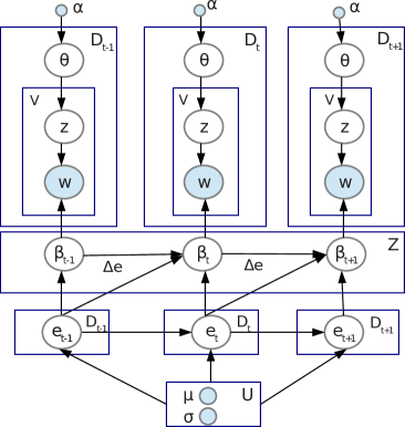
Figure IV.8: Continuous experience-aware language model. Words (shaded in blue), and timestamps (not shown for brevity) are observed.

1. Set granularity $t$ for language model evolution (e.g., years, months, days)

2. Set granularity for experience evolution, timestamp $t^{\prime}$ (e.g., minutes, seconds)

for each coarse timepoint t do

       for each review $d\in D_{t}$ do

             // retrieve user $u=u_{d}$ and fine-grained timepoint $t^{\prime}=t^{\prime}_{d}$

             3. Draw $e_{d}\sim\text{Log-Normal}((\mu_{u}-\frac{\sigma_{u}^{2}}{2})t{{}^{\prime}}+log(s_{0,u}),\sigma_{u}\sqrt{t{{}^{\prime}}})$

             4. Draw $\theta_{d}\sim\text{Dirichlet}(\alpha)$

             for each word $w$ in $d$ do

                   5. Draw $z_{d,w}\sim\text{Multinomial}(\theta_{d}$)

                  

             end for

            

       end for

      6. Draw $\beta_{t,z,w}\sim\text{Normal}(\beta_{t-1,z,w},\sigma\cdot|l_{t,w}-l_{t-1,w}|)$

       for each review $d\in D_{t}$ do

             for each word $w$ in $d$ do

                   7. Draw $w\sim\text{Multinomial}(\pi(\beta_{t_{d},z_{d,w}}))$

             end for

            

       end for

      

end for

Algorithm 3 Generative model for continuous experience-aware language model.

Inference

Let $E,L,Z,T$ and $W$ be the set of experience values of all reviews, experience values of words, facets, timestamps and words in the corpus, respectively. In the following, $d$ denotes a review and $j$ indexes a word in it. $\theta$ denotes the per-review facet distribution, and $\beta$ the language model respectively.

The joint probability distribution is given by:

$$P(E,L,Z,W,\theta,\beta|U,T;\alpha,\langle\mu\rangle,\langle\sigma\rangle)\propto\\ \prod_{t\in T}\prod_{d\in D_{t}}P(e_{d};s_{0,u_{d}},\mu_{u_{d}},\sigma_{u_{d}})\boldsymbol{\cdot}\bigg{(}P(\theta_{d};\alpha)\cdot\prod_{j=1}^{N_{d}}P(z_{d,j}|\theta_{d})\cdot P(w_{d,j}|\pi(\beta_{z_{d,j},t}))\bigg{)}\\ \boldsymbol{\cdot}\bigg{(}\prod_{z\in Z}\prod_{w\in W}P(l_{t,w};e_{d})\cdot P(\beta_{t,z,w};\beta_{t-1,z,w},\sigma\cdot|l_{t,w}-l_{t-1,w}|)\bigg{)}\\$$ (IV.13)

The exact computation of the above distribution is intractable, and we have to resort to approximate inference.

Exploiting conjugacy of the Multinomial and Dirichlet distributions, we can integrate out $\theta$ from the above distribution. Assuming $\theta$ has been integrated out, we can decompose the joint distribution as:

$$P(Z,\beta,E,L|W,T)\propto P(Z,\beta|W,T)\cdot P(E|Z,\beta,W,T)\cdot P(L|E,W,T)$$ (IV.14)

The above decomposition makes certain conditional independence assumptions in line with our generative process.

Estimating Facets $Z$: We use Collapsed Gibbs Sampling [Griffiths 2002], as in standard LDA, to estimate the conditional distribution for each of the latent facets $z_{d,j}$, which is computed over the current assignment for all other hidden variables, after integrating out $\theta$. Let $n(d,z)$ denote the count of the topic $z$ appearing in review $d$. In the following equation, $n(d,.)$ indicates the summation of the above counts over all possible $z\in Z$. The subscript $-j$ denotes the value of a variable excluding the data at the $j^{th}$ position.

The posterior distribution $P(Z|\beta,W,T;\alpha)$ of the latent variable $Z$ is given by:

$$P(z_{d,j}=k|z_{d,-j},\beta,w_{d,j},t,d;\alpha)$$ (IV.15)

$$\propto\frac{n(d,k)+\alpha}{n(d,.)+Z\cdot\alpha}\boldsymbol{\cdot}P(w_{n}=w_{d,j}|\beta,t,z_{n}=k,z_{-n},w_{-n})$$

$$=\frac{n(d,k)+\alpha}{n(d,.)+Z\cdot\alpha}\boldsymbol{\cdot}\pi(\beta_{t,k,w_{n}})$$

where, the transformation $\pi$ is given by Equation IV.10.

Estimating Language Model $\beta$: In contrast to $\theta$, the variable $\beta$ cannot be integrated out by the same process, as Normal and Multinomial distributions are not conjugate. Therefore, we refer to another approximation technique to estimate $\beta$.

In this work, we use Kalman Filter [Kalman 1960] to model the sequential language model evolution. It is widely used to model linear dynamic systems from a series of observed measurements over time, containing statistical noise, that produces robust estimates of unknown variables over a single measurement. It is a continuous analog to the Hidden Markov Model (HMM), where the state space of the latent variables is continuous (as opposed to the discrete state-space HMM); and the observed and latent variables evolve with Gaussian noise.

We want to estimate the following state-space transition model:

$$\beta_{t,z,w}|\beta_{t-1,z,w} \sim N(\beta_{t-1,z,w},\sigma\cdot|l_{t,w}-l_{t-1,w}|)$$ (IV.16)

$$w_{d,j}|\beta_{t,z,w} \sim Mult(\pi(\beta_{t,z,w}))\text{\hskip 10.00002ptwhere, }z=z_{d,j},t=t_{d}.$$

However, unlike standard Kalman Filter, we do not have any observed measurement of the variables — due to the presence of latent facets $Z$. Therefore, we resort to inferred measurement from the Gibbs sampling process.

Let $n(t,z,w)$ denote the number of times a given word $w$ is assigned to a facet $z$ at time $t$ in the corpus. Therefore,

$$\beta^{inf}_{t,z,w}=\pi^{-1}\bigg{(}\frac{n(t,z,w)+\gamma}{n(t,z,.)+V\cdot\gamma}\bigg{)}$$ (IV.17)

where, we use the inverse transformation of $\pi$ given by Equation IV.10, and $\gamma$ is used for smoothing.

Update Equations for Kalman Filter: Let $p_{t}$ and $g_{t}$ denote the prediction error, and Kalman Gain at time $t$ respectively. The variance of the process noise and measurement is given by the difference of the experience value of the word observed at two successive timepoints. Following standard Kalman Filter calculations [Kalman 1960], predict equations are given by:

$$\widehat{\beta}_{t,z,w} \sim N(\beta_{{t-1},z,w},\sigma\cdot|l_{t,w}-l_{t-1,w}|)$$ (IV.18)

$$\widehat{p}_{t} =p_{t-1}+\sigma\cdot|l_{t-1,w}-l_{t-2,w}|$$

and the update becomes:

$$g_{t} =\frac{\widehat{p}_{t}}{\widehat{p}_{t}+\sigma\cdot|l_{t,w}-l_{t-1,w}|}$$ (IV.19)

$$\beta_{t,z,w} =\widehat{\beta}_{t,z,w}+g_{t}\cdot(\beta^{inf}_{t,z,w}-\widehat{\beta}_{t,z,w})$$

$$p_{t} =(1-g_{t})\cdot\widehat{p}_{t}$$

Thus, the new value for $\beta_{t,z,w}$ is given by Eq. IV.19.

If the experience does not change much between two successive timepoints, i.e. the variance is close to zero, the Kalman Filter just emits the counts as estimated by Gibbs sampling (assuming, $P_{0}=1$). This is then similar to the Dynamic Topic Model [Blei 2006]. Intuitively, the Kalman Filter is smoothing the estimate of Gibbs sampling taking the experience evolution into account.

Estimating Experience $E$: The experience value of a review depends on the user and the language model $\beta$. Although we have the state-transition model of $\beta$, the previous process of estimation using Kalman Filter cannot be applied in this case, as there is no observed or inferred value of $E$. Therefore, we resort to Metropolis Hastings sampling. Instead of sampling the $E$’s from the complex true distribution, we use a proposal distribution for sampling the random variables — followed by an acceptance or rejection of the newly sampled value. That is, at each iteration, the algorithm samples a value of a random variable — where the current estimate depends only on the previous estimate, thereby, forming a Markov chain.

Assume all reviews $\{\cdots d_{i-1},d_{i},d_{i+1}\cdots\}$ from all users are sorted according to their timestamps. As discussed in Section IV.4.1, for computational feasibility, we use a coarse granularity for the language model $\beta$. For the inference of $E$, however, we need to operate at the fine temporal resolution of the reviews’ timestamps (say, in minutes or seconds). Note that the process defined in Eq. (IV.12) represents the aggregated language model over multiple fine-grained timestamps. Accordingly, its corresponding fine-grained counterpart is $\beta_{t^{\prime}_{d_{i}},z,w}\sim Normal(\beta_{t^{\prime}_{d_{i-1}},z,w},\sigma\cdot|e_{d_{i}}-e_{d_{i-1}}|)$ — now operating on $t^{\prime}$ and the review’s individual experience values. Since the language model is given (i.e. previously estimated) during the inference of $E$ , we can now easily refer to this fine-grained definition for the Metropolis Hastings sampling.

As the proposal distribution for the experience of review $d_{i}$ at time $t^{\prime}_{d_{i}}$ , we select the corresponding user’s GBM ($u=u_{d}$) and sample a new experience value $\widehat{e_{d_{i}}}$ for the review:

$$\widehat{e}_{d_{i}}\sim\text{Log-Normal}((\mu_{u}-\frac{\sigma_{u}^{2}}{2})t^{\prime}_{d_{i}}+log(s_{0,u}),\sigma_{u}\sqrt{t^{\prime}_{d_{i}}})$$

The language model $\beta_{t^{\prime}_{d_{i}}}$ at time $t^{\prime}_{d_{i}}$ depends on the language model $\beta_{t^{\prime}_{d_{i-1}}}$ at time $t^{\prime}_{d_{i-1}}$, and experience value difference $|e_{d_{i}}-e_{d_{i-1}}|$ between the two timepoints. Therefore, a change in the experience value at any timepoint affects the language model at the current and next timepoint, i.e. $\beta_{t^{{}^{\prime}}_{d_{i+1}}}$ is affected by $\beta_{t^{{}^{\prime}}_{d_{i}}}$, too.

Thus, the acceptance ratio of the Metropolis Hastings sampling becomes:

$$Q=\prod_{w,z}\bigg{[}\frac{N(\beta_{t^{\prime}_{b},z,w};\beta_{t^{\prime}_{a},z,w},\sigma\cdot|\widehat{e_{b}}-e_{a}|)}{N(\beta_{t^{\prime}_{b},z,w};\beta_{t^{\prime}_{a},z,w},\sigma\cdot|e_{b}-e_{a}|)}\boldsymbol{\cdot}\frac{N(\beta_{t^{\prime}_{c},z,w};\beta_{t^{\prime}_{b},z,w},\sigma\cdot|e_{c}-\widehat{e_{b}}|)}{N(\beta_{t^{\prime}_{c},z,w};\beta_{t^{\prime}_{b},z,w},\sigma\cdot|e_{c}-e_{b}|)}\bigg{]}$$ (IV.20)

where $a=d_{i-1}$, $b=d_{i}$ and $c=d_{i+1}$. The numerator accounts for the modified distributions affected by the updated experience value, and the denominator discounts the old ones. Note that since the GBM has been used as the proposal distribution, its factor cancels out in the term $Q$.

Overall, the Metropolis Hastings algorithm iterates over the following steps:

1. Randomly pick a review $d$ at time $t^{\prime}=t^{\prime}_{d}$ by user $u=u_{d}$ with experience $e_{d}$

2. Sample $\widehat{e_{d}}\sim\text{Log-Normal}\bigg{(}(\mu_{u}-\frac{\sigma_{u}^{2}}{2})t^{\prime}+log(s_{0,u}),\sigma_{u}\sqrt{t^{\prime}}\bigg{)}$

3. Accept $\widehat{e_{d}}$ as the new experience with probability $P$ $=$ $min(1,Q)$

Estimating Parameters for the Geometric Brownian Motion: For each user $u$, the mean $\mu_{u}$ and variance $\sigma_{u}$ of her GBM trajectory are estimated from the sample mean and variance.

Consider the set of all reviews $\langle d_{t}\rangle$ written by $u$, and $\langle e_{t}\rangle$ be the corresponding experience values of the reviews.

Let $\widehat{m}_{u}=\frac{\sum_{d_{t}}log(e_{t})}{|d_{t}|}$, and $\widehat{s}_{u}^{2}=\frac{\sum_{d_{t}}(log(e_{t})-\widehat{m}_{u})^{2}}{|d_{t}-1|}$.

Furthermore, let $\Delta$ be the average length of the time intervals for the reviews of user $u$.

Now, $log(e_{t})\sim N\big{(}(\mu_{u}-\frac{\sigma_{u}^{2}}{2})\Delta+log(s_{0,u}),\sigma_{u}\sqrt{\Delta}\big{)}$.

From the above equations we can obtain the following estimates using Maximum Likelihood Estimation (MLE):

$$\widehat{\sigma}_{u} =\frac{\widehat{s}_{u}}{\sqrt{\Delta}}$$ (IV.21)

$$\widehat{\mu}_{u} =\frac{\widehat{m}_{u}-log(s_{0,u})}{\Delta}+\frac{{\widehat{\sigma}_{u}}^{2}}{2}$$

$$=\frac{\widehat{m}_{u}-log(s_{0,u})}{\Delta}+\frac{{\widehat{s}_{u}}^{2}}{2\Delta}$$

Overall Processing Scheme: Exploiting the results from the above discussions, the overall inference is an iterative process consisting of the following steps:

1. Estimate facets $Z$ using Equation IV.15.

2. Estimate $\beta$ using Equations IV.18 and IV.19.

3. Sort all reviews by timestamps, and estimate $E$ using Equation IV.20 and the Metropolis Hastings algorithm, for a random subset of the reviews.

4. Once the experience values of all reviews have been determined, estimate $L$ using Equation IV.11.

IV.4.3 Experiments

We perform experiments with data from five communities in different domains:

• BeerAdvocate (beeradvocate.com) and RateBeer (ratebeer.com) for beer reviews

• Amazon (amazon.com) for movie reviews

• Yelp (yelp.com) for food and restaurant reviews

• NewsTrust (newstrust.net) for reviews of news media

Table IV.7 gives the dataset statistics. We have a total of $12.7$ million reviews from $0.9$ million users over $16$ years from all of the five communities combined. The first four communities are used for product reviews, from where we extract the following quintuple for our model $<userId,itemId,timestamp,rating,review>$. NewsTrust is a special community, which we discuss in Section IV.5.

Dataset	#Users	#Items	#Ratings	#Years
Beer (BeerAdvocate)	33,387	66,051	1,586,259	16
Beer (RateBeer)	40,213	110,419	2,924,127	13
Movies (Amazon)	759,899	267,320	7,911,684	16
Food (Yelp)	45,981	11,537	229,907	11
Media (NewsTrust)	6,180	62,108	89,167	9
TOTAL	885,660	517,435	12,741,144	-

Table IV.7: Dataset statistics.

Data Likelihood, Smoothness and Convergence

Inference of our model is quite involved with different Markov Chain Monte Carlo methods. It is imperative to show that the resultant model is not only stable, but also improves the log-likelihood of the data. Although there are several measures to evaluate the quality of facet models, we report the following from [Wallach 2009]:
$LL=\sum_{d}\sum_{j=1}^{N_{d}}log\ P(w_{d,j}|\beta;\alpha)$. A higher likelihood indicates a better model.

Figure IV.9 contrasts the log-likelihood of the data from the continuous experience model and its discrete counterpart (refer to Section IV.3). We find that the continuous model is stable and has a smooth increase in the data log-likelihood per iteration. This can be attributed to how smoothly the language model evolves over time, preserving the Markov property of experience evolution. Empirically our model also shows a fast convergence, as indicated by the number of iterations.

On the other hand, the discrete model not only has a worse fit, but is also less smooth. It exhibits abrupt state transitions in the Hidden Markov Model, when the experience level changes (refer to Figure IV.7). This leads to abrupt changes in the language model, as it is coupled to experience evolution.

Experience-aware Item Rating Prediction

In the first task, we show the effectiveness of our model for item rating prediction. Given a user $u$, an item $i$, time $t$, and review $d$ with words $\langle w\rangle$ — the objective is to predict the rating the user would assign to the item based on her experience.

For prediction, we use the following features: The experience value $e$ of the user is taken as the last experience attained by the user during training. Based on the learned language model $\beta$, we construct the language feature vector $\langle F_{w}=log(max_{z}(\beta_{t,z,w}))\rangle$ of dimension $V$ (size of the vocabulary). That is, for each word $w$ in the review, we consider the value of $\beta$ corresponding to the best facet $z$ that can be assigned to the word at the time $t$. We take the log-transformation of $\beta$ which empirically gives better results.

Furthermore, as also done in the baseline works [McAuley 2013b] and the discrete version of our model (refer to Section IV.3), we consider: $\gamma_{g}$, the average rating in the community; $\gamma_{u}$, the offset of the average rating given by user $u$ from the global average; and $\gamma_{i}$, the rating bias for item $i$.

Thus, combining all of the above, we construct the feature vector $\langle\langle F_{w}\rangle,e,\gamma_{g},\gamma_{u},\gamma_{i}\rangle$ for each review with the user-assigned ground rating for training. We use Support Vector Regression [Drucker 1996], with the same set of default parameters as used in our discrete model (refer to Section IV.3), for rating prediction.

Models	BeerAdvocate	RateBeer	NewsTrust	Amazon	Yelp
Continuous experience model	0.247	0.266	0.494	1.042	0.940
(this work)
Discrete experience model	0.363	0.309	0.464	1.174	1.469
(Section IV.3)
User at learned rate	0.379	0.336	0.575	1.293	1.732
[McAuley 2013b]
Community at learned rate	0.383	0.334	0.656	1.203	1.534
[McAuley 2013b]
Community at uniform rate	0.391	0.347	0.767	1.203	1.526
[McAuley 2013b]
User at uniform rate	0.394	0.349	0.744	1.206	1.613
[McAuley 2013b]
Latent factor model	0.409	0.377	0.847	1.248	1.560
[Koren 2015]

Table IV.8: Mean squared error (MSE) for rating prediction. Our model performs better than competing methods.

Figure IV.9: Log-likelihood per iteration of discrete model (refer to Section IV.3) vs. continuous experience model (this work).

Baselines: We consider the following baselines [b – e] from [McAuley 2013b], and use their code for experiments. Baseline (f) is our prior discrete experience model (refer to Section IV.3).

• LFM: A standard latent factor recommendation model [Koren 2008].

• Community at uniform rate: Users and products in a community evolve using a single “global clock” [Koren 2010, Xiong 2010, Xiang 2010], where the different stages of the community evolution appear at uniform time intervals.

• Community at learned rate: This extends b) by learning the rate at which the community evolves with time, eliminating the uniform rate assumption.
  

• User at uniform rate: This extends b) to consider individual users, by modeling the different stages of a user’s progression based on preferences and experience levels evolving over time. The model assumes a uniform rate for experience progression.

• User at learned rate: This extends d) by allowing the experience of each user to evolve on a “personal clock”, where the time to reach certain (discrete) experience levels depends on the user [McAuley 2013b]. This is reportedly the best version of their experience evolution models.

• Discrete experience model: This is our prior approach (refer to Section IV.3) for the discrete version of the experience-aware language model, where the experience of a user depends on the evolution of the user’s maturing rate, facet preferences, and writing style.

Quantitative Results

Table IV.8 compares the mean squared error (MSE) for rating predictions in this task, generated by our model versus the six baselines. Our model outperforms all baselines — except in the NewsTrust community, performing slightly worse than our prior discrete model (discussed in Section IV.5) — reducing the MSE by ca. $11\%$ to $36\%$. Our improvements over the baselines are statistically significant at $99\%$ level of confidence determined by paired sample t-test.

For all models, we used the three most recent reviews of each user as withheld test data. All experience-based models consider the last experience value reached by each user during training, and the corresponding learned parameters for rating prediction. Similar to the setting in [McAuley 2013b], we consider users with a minimum of $50$ reviews. Users with less than $50$ reviews are grouped into a background model, and treated as a single user. We set $Z=5$ for BeerAdvocate, RateBeer and Yelp facets; and $Z=20$ for Amazon movies and $Z=100$ for NewsTrust which have richer latent dimensions. All discrete experience models consider $E=5$ experience levels. In the continuous model, the experience value $e\in(0,\infty)$. We initialize the parameters for our joint model as: $s_{0,u}=1,\alpha=50/Z,\gamma=0.01$. Our performance improvement is strong for the BeerAdvocate community due to large number of reviews per-user for a long period of time, and low for NewsTrust for the converse.

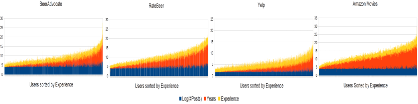
Figure IV.10:  Variation of experience ($e$) with years and reviews of each user. Each bar in the above stacked chart corresponds to a user with her most recent experience, number of years spent, and number of reviews posted in the community.

Figure IV.11:  Variation of experience ($e$) with mean ($\mu_{u}$) and variance ($\sigma_{u}$) of the GBM trajectory of each user ($u$). Each bar in the above stacked chart corresponds to a user with her most recent experience, mean and variance of her experience evolution.

Figure IV.12:  Variation of word frequency with word experience. Each point in the above scatter plot corresponds to a word ($w$) in “2011” with corresponding frequency and experience value ($l_{t\text{=2011},w}$).

Figure IV.13:  Language model score ($\beta_{t,z,w}\boldsymbol{\cdot}l_{t,w}$) variation for sample words with time. Figure a) shows the count of some sample words over time in BeerAdvocate community, whose evolution is traced in Figure b). Figures c) and d) show the evolution in Yelp and Amazon Movies.

Qualitative Results

User experience progression: Figure IV.10 shows the variation of the users’ most recent experience (as learned by our model), along with the number of reviews posted, and the number of years spent in the community. As we would expect, a user’s experience increases with the amount of time spent in the community. On the contrary, number of reviews posted does not have a strong influence on experience progression. Thus, if a user writes a large number of reviews in a short span of time, her experience does not increase much; in contrast to if the reviews are written over a long period of time.

Figure IV.11 shows the variation of the users’ most recent experience, along with the mean $\mu_{u}$ and variance $\sigma_{u}$ of her Geometric Brownian Motion (GBM) trajectory — all learned during inference. We observe that users who reach a high level of experience progress faster (i.e. a higher value of $\mu_{u}$) than those who do not. Experienced users also exhibit comparatively higher variance than amateur ones. This result also follows from using the GBM process, where the mean and variance tend to increase with time.

Language model evolution: Figure IV.12 shows the variation of the frequency of a word — used in the community in “2011” — with the learned experience value $l_{t,w}$ associated to each word. The plots depict a bell curve. Intuitively, the experience value of a word does not increase with general usage; but increases if it has been used by experienced users. Highlighted words in the plot give some interesting insights. For instance, the words “beer, head, place, food, movie, story” etc. are used with high frequency in the beer, food or movie community, but have an average experience value. On the other hand specialized words like “beeradvocate, budweiser, %abv, fullness, encore, minb&w” etc. have high experience value.

Table IV.9 shows some top words used by experienced users and amateur ones in different communities, as learned by our model. Note that this is a ranked list of words with numeric values (not shown in the table). We see that experienced users are more interested about fine-grained facets like the mouthfeel, “fruity” flavors, and texture of food and drinks; narrative style of movies, as opposed to popular entertainment themes; discussing government policies and regulations in news reviews etc.

The word “rex” in Figure IV.12 in Yelp, appearing with low frequency and high experience, corresponds to a user “Rex M.” with “Elite” status who writes humorous reviews with self reference.

Figure IV.13 shows the evolution of some sample words over time and experience (as given by our model) in different communities. The score in the y-axis combines the language model probability $\beta_{t,z,w}$ with experience value $l_{t,w}$ associated to each word $w$ at time $t$.

Figure IV.13 a) illustrates the frequency of the words in BeerAdvocate, while their evolution is traced in Figure IV.13 b). It can be seen that the overall usage of each word increases over time; but the evolution path is different for each word. For instance, the “smell” convention started when “aroma” was dominant; but the latter was less used by experienced users over time, and slowly replaced by (increasing use of) “smell”. This was also reported in [Danescu-Niculescu-Mizil 2013] in a different context. Similarly “caramel” is likely to be used more by experienced users, than “flavor”. Also, contrast the evolution of “bitterness”, which is used more by experienced users, compared to “bitter”.

In Yelp, we see certain food trends like “grilled” and “crispy” increasing over time; in contrast to a decreasing feature like “casino” for restaurants. For Amazon movies, we find certain genres like “horror, thriller” and “contemporary” completely dominating other genres in recent times.

Most Experience	Least Experience
BeerAdvocate
chestnut_hued near_viscous rampant_perhaps faux_foreign cherry_wood sweet_burning bright_crystal faint_vanilla boned_dryness woody_herbal citrus_hops mouthfeel	originally flavor color didnt favorite dominated cheers tasted review doesnt drank version poured pleasant bad bitter sweet
Amazon
aficionados minimalist underwritten theatrically unbridled seamless retrospect overdramatic diabolical recreated notwithstanding oblivious featurettes precocious	viewer entertainment battle actress tells emotional supporting evil nice strong sex style fine hero romantic direction superb living story
Yelp
rex foie smoked marinated savory signature contemporary selections bacchanal delicate grits gourmet texture exotic balsamic	mexican chicken salad love better eat atmosphere sandwich local dont spot day friendly order sit
NewsTrust
health actions cuts medicare oil climate major jobs house vote congressional spending unemployment citizens events	bad god religion iraq responsibility questions clear jon led meaningful lives california powerful

Table IV.9:  Top words used by experienced and amateur users.

IV.5 Use-Case Study

Sections IV.3 and IV.4 discuss the evolution of user experience in online communities — with applications focused on recommending items (like beers or movies) to users based on their maturity. As another application use-case, we switch to a different kind of items – newspapers and news articles – tapping into the NewsTrust online community (newstrust.net). NewsTrust features news stories posted and reviewed by members, many of whom are professional journalists and content experts. Stories are reviewed based on their objectivity, rationality, and general quality of language to present an unbiased and balanced narrative of an event. The focus is on quality journalism. Unlike the other datasets, NewsTrust contains expertise of members that can be used as ground-truth for evaluating our model-generated experience values of users. Previously in Section III.7.1, we had discussed several characteristics of this community that were employed for credibility analysis therein.

In our framework of item recommendation, each story is an item, which is rated and reviewed by a user. The facets are the underlying topic distribution of reviews, with (latent) topics being Healthcare, Obama Administration, NSA, etc. The facet preferences can be mapped to the (political) polarity of users in the news community.

IV.5.1 Recommending News Articles

Our first objective is to recommend news to readers catering to their facet preferences, viewpoints, and experience. We apply our joint model to this task, and compare the predicted ratings with the ones observed for withheld reviews in the NewsTrust community.

The mean squared error (MSE) results for this task were reported in Table IV.8. Our continuous model clearly outperforms most of the baselines; it performs only slightly worse regarding our prior discrete model (discussed in Section IV.3) in this task — possibly due to high rating / data sparsity in face of a large number of model parameters and less number of reviews per-user.

Table IV.10 shows salient examples of the vocabulary by users at different (discrete) experience levels on the topic US Election as generated by the discrete version of our model (refer to Section IV.3).

Level 1: bad god religion iraq responsibility

Level 2: national reform live krugman questions clear jon led meaningful lives california powerful safety impacts

Level 3: health actions cuts medicare nov news points oil climate major jobs house high vote congressional spending unemployment strong taxes citizens events failure

Table IV.10:  Salient words for the illustrative NewsTrust topic US Election used by users at different levels of experience.

IV.5.2 Identifying Experienced Users

Our second task is to find experienced members of this community, who have the potential of being citizen journalists. In order to evaluate the quality of the ranked list of experienced users generated by our model, we consider the following proxy measure for user experience. In NewsTrust, users have Member Levels determined by the NewsTrust staff based on community engagement, time in the community, other users’ feedback on reviews, profile transparency, and manual validation.

We use these member levels to categorize users as experienced or inexperienced. This is treated as the ground truth for assessing the ranking quality of our model against the baseline models [McAuley 2013b], and the discrete version of our prior work (discussed in Section IV.3) — considering top $100$ users from each model ranked by experience. Here we consider the top-performing baseline models from the previous task.

We report the Normalized Discounted Cumulative Gain (NDCG) and the Normalized Kendall Tau Distance for the ranked lists of users generated by all the models. NDCG gives geometrically decreasing weights to predictions at the various positions of the ranked list:

$NDCG_{p}=\frac{DCG_{p}}{IDCG_{p}}$,     where $DCG_{p}=rel_{1}+\sum_{i=2}^{p}\frac{rel_{i}}{\log_{2}i}$

Here, $rel_{i}$ is the relevance ($0$ or $1$) of a result at position $i$.

The better model should exhibit higher NDCG, and lower Kendall Tau Distance.

As Table IV.11 shows, the continuous version of our model performs better than its discrete counterpart, which, in turn, outperforms [McAuley 2013b] in capturing user maturity.

Models	NDCG	Kendall Tau
		Normalized Distance
Continuous experience model (this work)	0.917	0.113
Discrete experience model (refer to Section IV.3)	0.898	0.134
User at learned rate [McAuley 2013b]	0.872	0.180

Table IV.11:  Performance on identifying experienced users.

IV.6 Conclusion

In this chapter, we propose models to capture the temporal evolution of users in online communities. These can be used to identify users who were not experienced when they joined the community, but could have evolved into a matured user now. Current recommender systems do not consider the temporal dynamics of user experience when generating recommendations. We propose experience-aware recommendation models — that can adapt to the changing preferences and maturity of users in a community — to recommend items that she will appreciate at her current maturity level. We exploit the coupling between the facet preferences of a user, her experience, writing style in reviews, and rating behavior to capture the user’s temporal evolution. Our model is the first work that considers the progression of users’ experience as expressed in the text of item reviews.

Furthermore, we develop an experience-aware language model that can trace the continuous evolution of a user’s experience and her language explicitly over time. We combine principles of Geometric Brownian Motion, Brownian Motion, and Latent Dirichlet Allocation to model a smooth temporal progression of user experience, and language model over time. This is also the first work to develop a continuous and generalized version of user experience evolution.

We derive interesting insights from the evolution trajectory of users, and their vocabulary usage with change in experience. For instance, experienced users progress faster than amateurs, with the progression depending more on their time spent in the community than on activity. Experienced users also show a more predictable behavior, and have a distinctive writing style and facet preferences — for example, experienced users in the Beer community use more “fruity” words to depict the smell and taste of a beer; and users in the News community are more interested about policies and regulations than amateurs who are more interested in polarizing topics.

Our experiments – with data from domains like beer, movies, food, and news – demonstrate that our model effectively exploits user experience for item recommendation that substantially reduces the mean squared error for predicted ratings, compared to the state-of-the-art baselines. This shows our method can generate better recommendations than those models.

We further demonstrate the utility of our model in a use-case study on identifying experienced members in the NewsTrust community, where these users would be top candidates for being citizen journalists. Another similar use-case for our model can be to detect experienced medical professionals in the health community who can contribute valuable medical knowledge.

Credibility Analysis of Product Reviews

V.1 Introduction

Chapters III and IV develop probabilistic graphical models for credibility analysis in online communities and their temporal evolution, respectively. In the current chapter, we use the principles and models developed therein for some related tasks that have been of serious concern for product review communities in recent times.

With the rapid growth in e-Commerce, product reviews have become a crucial component for the business nowadays. As consumers cannot test the functionality of a product prior to purchase, these reviews help them make an informed decision to buy the product or not. As per the survey conducted by Nielsen Corporations, $40\%$ of online consumers have indicated that they would not buy electronics without consulting online reviews first [Nielsen]. Due to the increasing dependency on user-generated reviews, it is crucial to understand their quality — that can widely vary from being an excellent-detailed opinion to superficial criticizing or praising, to spams in the worst case. Unfortunately, review forums such as TripAdvisor, Yelp, Amazon, and others are being increasingly game to manipulative and deceptive reviews: fake (to promote or demote some item), incompetent (rating an item based on irrelevant aspects), or biased (giving a distorted and inconsistent view of the item). For example, recent studies depict that $20\%$ of Yelp reviews might be fake and Yelp internally rejects $16\%$ of user submissions [Luca 2015] as “not-recommended”.

Recent research has proposed approaches to identify helpful reviews and spams automatically, but they suffer from major drawbacks: most of these approaches are geared towards active users and items in the community with a lot of reviews and activity information, and, therefore, not suitable for “long-tail” users and items with limited data. Most importantly, these works — based on crude user behavioral, and shallow textual features — do not provide any interpretable explanation as to why a review should be deemed helpful, or non-credible.

In order to address the above issues, we propose probabilistic approaches based on analyzing reviews on several aspects like consistency, (latent) semantics, and temporal dynamics for two tasks in online review communities: (i) finding useful product reviews that are helpful to the end consumers, and (ii) finding credible reviews with limited information about users and items, specifically, for the “long-tail” ones using consistency features. We provide user-interpretable explanations for our verdict for both the tasks.

V.2 Motivation and Approach

V.2.1 Finding Useful Product Reviews

Motivation: Online reviews provided by consumers are a valuable asset for e-Commerce platforms, influencing potential consumers in making purchasing decisions. However, without any indication of the review quality, it is overwhelming for consumers to browse through a multitude of reviews. In order to help consumers in finding useful reviews, most of the e-Commerce platforms nowadays allow users to vote whether a product review is helpful or not. For instance, any Amazon product review is accompanied with information like $x$ out of $y$ users found the review helpful. This helpfulness score ($x/y$) can be considered as a proxy for the review quality and its usefulness to the end consumers. In this task, we aim to automatically find the helpfulness score of a review based on certain consistency, and semantic aspects of the review like: whether the review is written by an expert, what are the important facets of the product outlined in his review, what do other experts have to say about the given product, timeliness of the review etc. — that are automatically mined as latent factors from review texts.

State-of-the-Art and its Limitations: Prior works on predicting review helpfulness mostly operate on shallow syntactic textual features like bag-of-words, part-of-speech tags, and tf-idf (term, and inverse document frequency) statistics [Kim 2006, Lu 2010]. These works, and other related works on finding review spams [Jindal 2008, Mukherjee 2013a] classify extremely opinionated reviews as not helpful. Similarly, other works exploiting rating & activity features like frequency of user posts, average ratings of users and items [O’Mahony 2009, Lu 2010, Liu 2007] consider extreme ratings and deviations as indicative of unhelpful reviews. Some recent works incorporate additional information like community-specific characteristics (who-voted-whom) with explicit user network [Tang 2013, Lu 2010], and item-specific meta-data like explicit item facets and product brands [Liu 2008, Kim 2006]. Apart from the requirement of a large number of meta-features that restrict the generalizability of many of these models to any arbitrary domain, these shallow features do not analyze what the review is about, and, therefore, cannot explain why it should be helpful for a given product. Some of these works [O’Mahony 2009, Liu 2008] identify expertise of a review’s author as an important feature. However, in absence of suitable modeling techniques, they consider prior reputation features like user activity, and low rating deviation as a proxy for user expertise.

The work closest to our approach is [Liu 2008] — where the authors identify syntactic features, user expertise, and timeliness of a review as important indicators of its quality. However, even in this case, the authors use part-of-speech tags as syntactic features, and user preferences for explicit item facets (pre-defined genres of IMDB movies in their work) as proxy for user expertise. In contrast, we explicitly model user expertise as a function of their writing style, rating style, and preferences for (latent) item facets — all of which are jointly learned from user-contributed reviews — going beyond the usage of shallow syntactic features, and the requirement for additional item meta-data.

Problem Statement: Our work aims to overcome the limitations of prior works by exploring the semantics and consistency of a review to predict its helpfulness score for a given item. Unlike prior works, all of these features can be harnessed from only the information of a user reviewing an item at an explicit timepoint, making our approach fairly general for all communities and domains. We also provide interpretable explanation in terms of latent word clusters that gives interesting insights as to what makes the review helpful.

Approach: The first step towards understanding the semantics of a review is to uncover the facet descriptions of the target item outlined in the review. We treat these facets as latent and use Latent Dirichlet Allocation (LDA) to discover them as topic clusters. The second step is to find the expertise of the users who wrote the review, and their description of the different (latent) facets of the item. Our approach in modeling user expertise is similar to that outlined in Chapter IV. However, there are significant differences and modifications (discussed in Section V.3.2) in modeling the joint interactions between several factors, where our proposed model has a better coupling between the factors, all of which are learned directly from the review helpfulness.

We make use of distributional hypotheses (outlined in Section V.3.1) like: expert users agree on what are the important facets of an item, and their description (or, writing style) of those facets influences the helpfulness of a review. We also derive several consistency features — all from the given quintuple $\langle$userId, itemId, rating, reviewText, timepoint$\rangle$ — like prior user reputation, item prominence, and timeliness of a review, that are used in conjunction with the semantic features. Finally, we leverage the interplay between all of the above factors in a joint setting to predict the review helpfulness.

For interpretable explanation, we derive interesting insights from the latent word clusters used by experts — for instance, reviews describing the underlying “theme and storytelling” of movies and books, the “style” of music, and “hygiene” of food are considered most helpful for the respective domains.

Contributions: The salient contributions of this work can be summarized as:

• Model: We propose an approach to leverage the semantics and consistency of reviews to predict their helpfulness. We propose a Hidden Markov Model – Latent Dirichlet Allocation (HMM-LDA) based model that jointly learns the (latent) item facets, (latent) user expertise, and his writing style from observed words in reviews at explicit timepoints.

• Algorithm: We introduce an effective learning algorithm based on an iterative stochastic optimization process that reduces the mean squared error of the predicted helpfulness scores with the ground scores, as well as maximizes the log-likelihood of the data.

• Experiments: We perform large-scale experiments with real-world datasets from five different domains in Amazon, together comprising of $29$ million reviews from $5.7$ million users on $1.9$ million items, and demonstrate substantial improvement over state-of-the art baselines for prediction and ranking tasks.

V.2.2 Finding Credible Reviews with Limited Information

Motivation: Starting with the work of [Jindal 2008], research efforts have been undertaken to automatically detect non-credible reviews. In parallel, industry (e.g., stakeholders such as Yelp) has developed its own standards to filter out “illegitimate” reviews. Although details are not disclosed, studies suggest that these filters tend to be fairly crude [Mukherjee 2013b]; for instance, exploiting user activity like the number of reviews posted, and treating users whose ratings show high deviation from the mean/majority ratings as suspicious. Such a policy seems to over-emphasize trusted long-term contributors and suppress outlier opinions off the mainstream. Moreover, these filters also employ several aggregated metadata, and are thus hardly viable for new items that initially have very few reviews — often by not so active users or newcomers in the community.

State-of-the-Art and Its Limitations: Research on this topic has cast the problem of review credibility into a binary classification task: a review is either credible or deceptive. To this end, supervised and semi-supervised methods have been developed that largely rely on features about users and their activities as well as statistics about item ratings. Most techniques also consider spatio-temporal patterns of user activities like IP addresses or user locations (e.g., [Li 2014a, Li 2015a]), burstiness of posts on an item or an item group (e.g., [Fei 2013]), and further correlation measures across users and items as discussed in Chapter III. However, the classifiers built this way are mostly geared for popular items, and the meta-information about user histories and activity correlations are not always available. For example, someone interested in opinions on a new art film or a “long-tail” bed-and-breakfast in a rarely visited town, is not helped at all by the above methods. Several existing works [Mihalcea 2009, Ott 2011, Ott 2013] consider the textual content of user reviews for tackling opinion spam by using word-level unigrams or bigrams as features, along with specific lexicons (e.g., LIWC [Pennebaker 2001] psycholinguistic lexicon, WordNet Affect [Strapparava 2004]), to learn latent topic models and classifiers (e.g., [Li 2013]). Although these methods achieve high classification accuracy for various gold-standard datasets, they do not provide any interpretable evidence as to why a certain review is classified as non-credible.

Problem Statement: This task focuses on detecting credible reviews with limited information, namely, in the absence of rich data about user histories, community-wide correlations, and for “long-tail” items. In the extreme case, we are provided with only the review texts and ratings for an item. Our goal is then to analyze various inconsistencies that may exist within the reviews — using which we can compute a credibility score and provide interpretable evidence for explaining why certain reviews have been categorized as non-credible.

Approach: Our proposed method to this end is to learn a model based on latent topic models and combining them with limited metadata to provide a novel notion of consistency features characterizing each review. We use the LDA-based Joint Sentiment Topic model (JST) [Lin 2009] to cast the user review texts into a number of informative facets. We do this per-item, aggregating the text among all reviews for the same item, and also per-review. This allows us to identify, score, and highlight inconsistencies that may appear between a review and the community’s overall characterization of an item. We perform this for the item as a whole, and also for each of the latent facets separately. Additionally, we learn inconsistencies such as discrepancy between the contents of a review and its rating, and temporal “bursts” — where a number of reviews are written in a short span of time targeting an item. We propose five kinds of inconsistencies that form the key assets of our credibility scoring model, fed into a Support Vector Machine for classification, or for ordinal ranking.

Contributions: In summary, our contributions are summarized as:

• Model: We develop a novel consistency model for credibility analysis of reviews that works with limited information, with particular attention to “long-tail” items, and offers interpretable evidence for reviews classified as non-credible.

• Tasks: We investigate how credibility scores affect the overall ranking of items. To address the scarcity of labeled training data, we transfer the learned model from Yelp to Amazon to rank top-selling items based on (classified) credible user reviews. In the presence of proxy labels for item “goodness” (e.g., item sales rank), we develop a better ranking model for domain adaptation.

• Experiments: We perform extensive experiments in TripAdvisor, Yelp, and Amazon to demonstrate the viability of our method and its advantages over state-of-the-art baselines in dealing with “long-tail” items and providing interpretable evidence.

V.3 Exploring Latent Semantic Factors to Find Useful Product Reviews

V.3.1 Review Helpfulness Factors

In this section, we outline the components of our model that analyze the semantics and consistency features of reviews, and show how these can help in predicting the review helpfulness.

Item Facets

Given a review on an item, it is essential to understand the different facets of the item described in the review. For instance, a camera review can focus on different facets like “resolution", “zoom", “price", “size”, or a movie review can focus on “narration", “cinematography", “acting", “direction” etc. However, not all facets are equally important for an item. For example, a review downrating a camera for “late delivery” by the seller is not as helpful to the general consumer as opposed to downrating it due to “grainy resolution” or “shaky zoom”. Therefore, a helpful review should focus on the important facets of an item. Another important aspect of a detailed review is to consider a wide range of facets of an item, rather than harping on a specific facet [Mudambi 2010, Kim 2006, Liu 2007].

Prior works [Liu 2007, Lu 2010, Kim 2006] consider the length distribution (like the number of words, sentences, or paragraphs in the review), and the overlap of explicit facets from the product description (including brand names, categories, specifications etc.) in the review as a proxy of how detailed it is.

In contrast, we model facets as latent variables, similar to that of a topic model [Blei 2001]. The latent facet distribution of an item in the review text is indicative of how detailed and diverse the review is.

Review Writing Style

Similar to the importance of the facets outlined in a review, the words used to describe the facets play a crucial role in making the review readable, and useful to the consumers. Due to diverse background of the reviewers with different language skills, the writing style too varies widely. An important aspect of an expert writing style is to use precise, domain-specific vocabulary to describe a facet in details, rather than using generic words. For instance, contrast this expert camera review:

Example V.3.1

60D focus screen is ‘grainy’. It is the ‘precision matte’ surface that helps to increase contrast and minimize depth of field for manual focusing. The Ef-s screen is even more so for use with fast primes. The T1i focus screen is smoother and brighter to compensate for the dimmer pentamirror design and typical economy f/3.5-5.6 zooms, but gives less precise manual focus.

with this amateur one:

Example V.3.2

This camera is pure garbage. This is the worst camera I have ever owned. I bought it last xmas on a deal and I have thrown it away and replaced it with a decent camera.

Another important factor to observe here is the balance in the reviewer’s opinion on an item. An expert review depicts a detailed judgment about the item, rather than just criticizing or praising it. Therefore, it is essential to distinguish the writing style of an experienced user from an amateur one.

Prior works [Jindal 2008, Kim 2006, Lu 2010, Liu 2007] capture the writing style from syntactic features like bag of words, part-of-speech tags, and use sentiment lexicons to find the distribution of positive and negative sentiment words in the review. In contrast, we learn a language model from the latent facets and user expertise that uncovers the hidden semantics in a review.

Reviewer Expertise

Previous works [Jindal 2008, O’Mahony 2009] in this domain attempted to harness a user’s expertise in writing a review under the hypothesis that expert reviews are positively correlated to review helpfulness. However, none of them explicitly modeled the users’ expertise. Instead, they considered the following proxy features for user reputation, namely:
Activity: Number of posts written by the user in the community.
Rating deviation: Deviation of the user rating from the community rating on an item.
Prior user reputation: Average number of helpfulness votes received by the user from her previous reviews.

In this work, we explicitly model user expertise adopting a similar approach as outlined in Section IV.3. However, we make substantial modifications (outlined in Section V.3.2) in modeling and learning the joint distributions conditioned on expertise — where all the distributions are explicitly learned from the review helpfulness scores as observables.

Unlike other factors in the model, expertise is not static, but evolves over time. A user who was not an expert at the time of entering the community, may have become an expert now contributing helpful reviews.

We model expertise as a latent variable that evolves over time, exploiting the hypothesis that users at similar levels of expertise have similar rating behavior, facet preferences, and writing style. The facets discovered in the previous step, and the writing style would therefore help us in finding a reviewer’s expertise. Once we figure out the reviewer’s expertise, we can find out the important facets of the item that he is concerned about, as well as the domain-specific vocabulary for describing the facets — thereby forming an effective feedback loop between facets, writing style, and expertise.

Distributional Hypotheses

Once we identify the (latent) item facets, (latent) expertise and preferences of different users, we can make use of the following hypotheses to capture the helpfulness of reviews:

• If the past reviews of a given user on an item (with a certain facet distribution) have been deemed helpful, then an incoming review by the given user on a similar kind of item (i.e. similar facet distribution) is also likely to be helpful. For instance, in the movie domain, if a user’s past reviews in the “drama” genre have been found to be helpful, and the movie under preview is also from the same genre, then its review is likely to be helpful.

• If the past reviews of users with certain characteristics (like, specific facet preferences and expertise) have been deemed helpful, and the given user has tastes and expertise similar to those users, then her current review is also likely to be helpful. For instance, assume we have learned how “expert” reviews in the “drama” genre looks like, and the current review text indicates the user to be an expert in the “drama” genre, then her review is likely to be helpful.

Note that in traditional collaborative filtering approaches for recommender systems, (i) and (ii) are similar to item-item and user-user similarities, respectively.

Consistency

Users and items do not gain reputation overnight. Therefore prior reputation of users and items are good indicators of the associated reviews’ helpfulness. In this work, we use the following consistency features that are used to guide our model to learn the latent distributions conditioned on the reviews’ helpfulness and ratings.

Prior user reputation: Average helpfulness votes received by the user’s past reviews from other users.
Prior item prominence: Average helpfulness votes received by the item’s past reviews from other users, which is also indicative of the prominence of the item.
User rating deviation: Absolute deviation between the user’s rating on an item, and the average rating assigned by the user over all other items. This captures the mean user rating behavior, and, therefore, scenarios where the user is too dis-satisfied (or, otherwise) with an item.
Item rating deviation: Absolute deviation between a user’s rating on the item, and average rating received by the item from all other users. This captures the scenario where a user unnecessarily criticizes or praises the item, that the community does not agree with.
Global rating deviation: Absolute deviation between the user’s rating on an item, and the average rating of all items by all users in the community. This captures the scenario where the user rating deviates from the general rating behavior of the community.

Timeliness or “Early-bird” bias

Prior work [Liu 2008] has shown a positive influence of a review’s publication date on the number of helpfulness votes received by it. The reason being that early and “timely” reviews are more useful to the consumers when the item is launched, so that they can make an informed decision about the item. Also, early reviews are exposed to consumers for a longer period of time which allows them to garner more votes over time, compared to recent reviews. The timestamp of the first review on a given item $i$ is considered to be the reference timepoint (say, $t_{i,0}$). Therefore, the timeliness of any other review on the item at time $t_{i}$ is computed as: $exp^{-(t_{i}-t_{i,0})}$.

Preliminary Study of Feature Significance

In order to understand the significance of different consistency features in predicting review helpfulness, we find correlation between various features described in the previous section and helpfulness scores of reviews. We consider reviews from five real-world datasets from Amazon in the domains namely, food, movies, music and electronics. We selected reviews that received a minimum of $five$ votes to maintain the robustness of the task.

Factors	Elect.	Foods	Music	Movies	Books
Item rating deviation	-0.364	-0.539	-0.596	-0.519	-0.516
Global rating deviation	-0.295	-0.507	-0.526	-0.439	-0.443
User rating deviation	-0.292	-0.429	-0.477	-0.267	-0.327
User activity	-0.056	0.002∗	-0.074	0.032	-0.033
Timeliness	0.036	0.083	0.102	0.114	0.137
Prior user reputation	0.062	0.191	0.353	0.525	0.386
Prior item prominence	0.221	0.251	0.343	0.303	0.343

Table V.1: Pearson correlation between different features and helpfulness scores of reviews in the domains electronics, foods, music, movies, and books. All factors (except the one marked with $*$) are statistically significant with p-value $<2e-16$.

From Table V.1, we observe that rating deviations — where the user diverges with the community rating on items, and her prior rating history — negatively impact helpfulness; whereas the prior reputation of users & items, and timeliness have a positive impact.

We also find that user activity alone does not have a significant impact on review helpfulness. In some cases (e.g., food domain) it is non-signifcant, or even has a negative impact on review helpfulness (e.g., electronics, music, and books domains). In order to find out if this feature fires in unison with other features, we use linear regression to predict the review helpfulness considering all of these features together. From the corresponding f-statistic we find user activity to be statistically significant with p-value $<2e-16$ in all cases (including the food domain) with a moderate positive weight. This feature, therefore, is used later in our expertise evolution model as a hyper-parameter that controls the rate of user progression.

Similarly, all of the other factors are reinforced in a joint setting, even though the correlations are quite low (for many of the features) in this study.

In the following section, we propose an approach to model all of these factors jointly to predict review helpfulness.

V.3.2 Joint Model for Review Helpfulness

Incorporating Consistency Factors

Let $u\in U$ be a user writing a review at time $t\in T$ on an item $i\in I$. Let $d=\{w_{1},w_{2},...w_{|N_{d}|}\}$ be the corresponding review text with a sequence of words $\langle w\rangle$, and rating $r\in R$. Each such review is associated with a helpfulness score $h\in[0-1]$. Let $b_{t}$ be the corresponding timeliness of the review computed as $exp^{-(t-t_{i,0})}$, where $t_{i,0}$ is the first review on the item $i$.

Let $\beta_{u}$ be the average helpfulness score of user $u$ over all the reviews written by her (capturing user reputation), and $\beta_{i}$ be the average helpfulness score of all reviews for item $i$ (capturing item prominence). Let $\overline{r}_{u}$ be the average rating assigned by the user over all items, $\overline{r}_{i}$ be the average rating assigned to the item by all users, and $\overline{r}_{g}$ be the average global rating over all items and users. Consistency features include prior item and user reputation, deviation features, and burst.

Let $\xi$ be a tensor of dimension $E\times Z$, where $E$ is the number of expertise levels of the users, and $Z$ is the number of latent facets of the items. $\xi_{e,z}$ depicts the opinion of users at (latent) expertise level $e\in E$ about the (latent) facet $z\in Z$. Therefore, the distributional hypotheses (outlined in the previous section) are intrinsically integrated in $\xi$ that is estimated from the reviews’ text, conditioned on the helpfulness score of the reviews.

The estimated helpfulness score $\widehat{h}(u,i)$ of a review by user $u$ on item $i$ is a function $f$ of the following consistency and latent factors, parametrized by $\Psi$:

$$\widehat{h}(u,i)=f(\beta_{u},\beta_{i},|r-\overline{r_{u}}|,|r-\overline{r_{i}}|,|r-\overline{r_{g}}|,b_{t},\xi;\Psi)$$ (V.1)

Here, $f$ can be a polynomial, radial basis, or a simple linear function for combining the features. The objective is to estimate the parameters $\Psi$ (of dimension: $6+E\times Z$) that reduces the mean squared error of the predicted helpfulness scores with the ground scores:

$$\Psi^{*}=argmin_{\Psi}\frac{1}{|U|}\sum_{u,i\in U,I}(h(u,i)-\widehat{h}(u,i))^{2}+\mu||\Psi||^{2}_{2}$$ (V.2)

where, we use $L_{2}$ regularization for the parameters to penalize complex models.

There are several ways to estimate the parameters like alternate least squares, gradient-descent, and Newton based approaches.

Incorporating Latent Facets

We use principles of Latent Dirichlet Allocation (LDA) [Blei 2001] to learn the latent facets associated to an item. Each review $d$ on an item is assumed to have a Multinomial distribution $\theta$ over facets $Z$ with a symmetric Dirichlet prior $\alpha$. Each facet $z$ has a Multinomial distribution $\phi_{z}$ over words drawn from a vocabulary $W$ with a symmetric Dirichlet prior $\delta$. Exact inference is not possible due to the intractable coupling between $\Theta$ and $\Phi$.

Two popular ways for approximate inference are MCMC techniques like Collapsed Gibbs Sampling and Variational Inference.

Incorporating Latent Expertise

Expertise influences both the facet distribution $\Theta$, as users at different levels of expertise have different facet preferences, and the language model $\Phi$ as the writing style is also different for users at different levels of expertise. Therefore, we parametrize both of these distributions with user expertise similar to our approach in Chapter IV.3, with some major modifications (discussed in the next section).

Consider $\Theta$ to be a tensor of dimension $E\times Z$, and $\Phi$ to be a tensor of dimension $E\times Z\times W$, where $\theta_{e,z}$ denotes the preference for facet $z\in Z$ for users at expertise level $e\in E$, and $\phi_{e,z,w}$ denotes the probability of the word $w\in W$ being used to describe the facet $z$ by users at expertise level $e$.

Now, expertise changes as users evolve over time. However, the transition should be smooth. Users cannot abruptly jump from expertise level $1$ to $4$ without passing through expertise levels $2$ and $3$. Therefore, at each timepoint $t+1$ (of posting a review), we assume a user at expertise level $e_{t}\in E$ to stay at $e_{t}$, or move to $e_{t}+1$ (i.e. expertise level is monotonically non-decreasing). This progression depends on how the writing style (captured by $\Phi$), and facet preferences (captured by $\Theta$) of the user is evolving with respect to other expert users in the community, as well as the rate of activity of the user. User activity is used as a proxy for expertise in many of the prior works [O’Mahony 2009, Lu 2010, Liu 2007]. However, we find it to play a weak role during our preliminary study. Therefore, we use it only as a hyper-parameter for controlling the rate of progression. Let $\gamma_{u}$, the activity rate of user $u$ be defined as: $\gamma_{u}=\frac{D_{u}}{D_{u}+D_{avg}}$, where $D_{u}$ and $D_{avg}$ denote the number of posts written by $u$, and the average number of posts written by any user in the community, respectively.

Let $\Pi$ be a tensor of dimension $E\times E$ with hyper-parameters $\langle\gamma_{u}\rangle$ of dimension $U$, where $\pi_{e_{i},e_{j}}$ denotes the probability of moving to expertise level $e_{j}$ from $e_{i}$ with the constraint $e_{j}\in\{e_{i},e_{i}+1\}$. However, not all users start at the same level of expertise, when they enter the community; some may enter already being an expert. The algorithm figures this out during the inference process. We assume all users to start at expertise level $1$ during parameter initialization.

During inference, we want to learn the parameters $\Psi,\xi,\Theta,\Phi,\Pi$ jointly for predicting review helpfulness.

Difference with Prior Works for Modeling Expertise

The generative process of user expertise has the following differences with our previous approach in Chapter IV.3:

• Previously we had learned user-specific preferences for personalized recommendation. However, we assume users at the same level of expertise to have similar facet preferences. Therefore, the facet distribution $\Theta$ is conditioned only on the user expertise, and not the user explicitly, unlike the prior works. This helps us to reduce the dimensionality of $\Theta$, and exploit the correspondence between $\Theta$ and $\xi$ to tie the parameters of the consistency and latent factor models together for joint inference.

• Our previous approach incorporates supervision, for predicting ratings, only indirectly via optimizing the Dirichlet hyper-parameters $\alpha$ of the Multinomial facet distribution $\Theta$ — and cannot guarantee an increase in the data log-likelihood over iterations. In contrast, we exploit (i) to learn the expertise-facet distribution $\Theta$ directly from the review helpfulness scores by minimizing the mean squared error during inference. This is also tricky as the parameters of the distribution $\Theta$, for an unconstrained optimization, are not guaranteed to lie on the simplex — for which we do certain transformations, discussed during inference. Therefore, the parameters are strongly coupled in our model, not only reducing the mean squared error, but also leading to a near smooth increase in the data log-likelihood over iterations (refer to Figure V.2).

Generative Process

Consider a corpus $D=\{d_{1},\ldots,d_{D}\}$ of reviews written by a set of users $U$ at timestamps $T$. For each review $d\in D$, we denote $u_{d}$ as its user, $t_{d}$ as the timestamp of the review. The reviews are assumed to be ordered by timestamps, i.e., $t_{d_{i}}<t_{d_{j}}$ for $i<j$. Each review $d\in D$ consists of a sequence of $N_{d}$ words denoted by $d=\{w_{1},\ldots,w_{N_{d}}\}$, where each word is drawn from a vocabulary $W$ having unique words indexed by $\{1\dots W\}$. Number of facets correspond to $Z$.

Let $e_{d}\in\{1,2,...,E\}$ denote the expertise value of review $d$. Since each review $d$ is associated with a unique timestamp $t_{d}$ and unique user $u_{d}$, the expertise value of a review refers to the expertise of the user at the time of writing it. Following Markovian assumption, the user’s expertise level transitions follow a distribution $\Pi$ with the Markovian assumption $e_{u_{d}}\sim\pi_{e_{u_{d-1}}}$ i.e. the expertise level of $u_{d}$ at time $t_{d}$ depends on her expertise level when writing the previous review at time $t_{d-1}$.

Once the expertise level $e_{d}$ of the user $u_{d}$ for review $d$ is known, her facet preferences are given by $\theta_{e_{d}}$. Thereafter, the facet $z_{d,w}$ of each word $w$ in $d$ is drawn from a Multinomial ($\theta_{e_{d}}$). Now that the expertise level of the user, and her facets of interest are known, we can generate the language model $\Phi$ and individual words in the review — where the user draws a word from the Multinomial distribution $\phi_{e_{d},z_{d,w}}$ with a symmetric Dirichlet prior $\delta$. Refer Figure V.1 for the generative process.

Figure V.1: Generative process for helpful product reviews.

The joint probability distribution is given by:

$$P(E,Z,W,\Theta,\Phi|U;\langle\gamma_{u}\rangle,\delta)\propto\prod_{u\in U}\prod_{d\in D_{u}}P(\pi_{e_{d}};\gamma_{u})\boldsymbol{\cdot}P(e_{d}|\pi_{e_{d}})\\ \boldsymbol{\cdot}\bigg{(}\prod_{j=1}^{N_{d}}P(z_{d,j}|\theta_{e_{d}})\cdot P(\phi_{e_{d},z_{d,j}};\delta)\cdot P(w_{d,j}|\phi_{e_{d},z_{d,j}})\bigg{)}$$ (V.3)

Inference

Given a corpus of reviews indexed by $\langle$userId, itemId, rating, reviewText, timepoint$\rangle$, with corresponding helpfulness scores, our objective is to learn the parameters $\Psi$ that minimizes the mean squared error given by Equation V.2.

In case $\xi$ was known, we could have directly plugged in its values (other features being observed) in Equation V.1 to learn a model (e.g., using regression) with parameters $\Psi$. However, the dimensions of $\xi$, corresponding to both facets and user expertise, are latent that need to be inferred from text. Now, the parameter weight $\psi_{e,z}$ corresponding to $\xi_{e,z}$ from Equation V.2 depicts the importance of the facet $z$ for users at expertise level $e$ for predicting review helpfulness. We want to exploit this observation to infer the latent dimensions from text.

During the generative process of a review document, for a user at expertise level $e$, we want to draw her facet of interest $z$ with probability $\theta_{e,z}\propto\psi_{e,z}$. However, we cannot directly replace $\Theta$ with $\Psi$ due to the following reason. The traditional parametrization of a Multinomial distribution ($\Theta$ in this case) is via its mean parameters. Any unconstrained optimization will take the parameters out of the feasible set, i.e. they may not lie on the simplex. Hence, it is easier to work with the natural parameters instead. If we consider the unconstrained parameters $\langle\psi_{e,z}\rangle$ (learned from Equation V.2) to be the natural parameters of the Multinomial distribution $\Theta$, we need to transform the natural parameters to the mean parameters that lie on the simplex (i.e. $\sum_{z}\theta_{e,z}=1$). In this work, we follow the same principle as in Equation IV.10 in Chapter IV.4 to do this transformation:

$$\theta_{e,z}=\frac{exp(\psi_{e,z})}{\sum_{z}exp(\psi_{e,z})}$$ (V.4)

where, $\psi_{e,z}$ corresponds to the learned parameter for $\xi_{e,z}$.

Exploiting conjugacy of the Multinomial and Dirichlet distributions, we can integrate out $\Phi$ from the joint distribution in Equation V.3 to obtain the posterior distribution $P(W|Z,E;\delta)$ given by:

$$\prod_{e=1}^{E}\prod_{z=1}^{Z}\frac{\Gamma(\sum_{w}\delta)\prod_{w}\Gamma(n(e,z,w)+\delta)}{\prod_{w}{\Gamma(\delta)\Gamma(\sum_{w}n(e,z,w)+\sum_{w}\delta)}}$$

where, $\Gamma$ denotes the Gamma function, and $n(e,z,w)$ is the number of times the word $w$ is used for facet $z$ by users at expertise level $e$.

We use Collapsed Gibbs Sampling [Griffiths 2002], as in standard LDA, to estimate the conditional distribution for each of the latent facets $z_{d,j}$, which is computed over the current assignment for all other hidden variables, after integrating out $\Phi$. In the following equation, $n(e,z,.)$ indicates the summation of the counts over all possible $w\in W$. The subscript $-j$ denotes the value of a variable excluding the data at the $j^{th}$ position.

The posterior distribution $P(Z|\Phi,W,E)$ of the latent variable $Z$ is given by:

$$P(z_{d,j}=k|z_{d,-j},\Phi,w_{d,j}=w,e_{d}=e,d)$$ (V.5)

$$\propto\theta_{e,k}\boldsymbol{\cdot}\frac{n(e,k,w)+\delta}{n(e,k,.)+W\cdot\delta}$$

$$=\frac{exp(\psi_{e,k})}{\sum_{z}exp(\psi_{e,z})}\boldsymbol{\cdot}\frac{n(e,k,w)+\delta}{n(e,k,.)+W\cdot\delta}$$

Similar to the above process, we use Collapsed Gibbs Sampling [Griffiths 2002] also to sample the expertise levels, keeping all facet assignments $Z$ fixed.

Let $n(e_{i-1},e_{i})$ denote the number of transitions from expertise level $e_{i-1}$ to $e_{i}$ over all users in the community, with the Markovian constraint $e_{i}\in\{e_{i-1},e_{i-1}+1\}$.

$$P(e_{i}|e_{i-1},e_{-i},u;\gamma_{u})=\frac{n(e_{i-1},e_{i})+I(e_{i-1}=e_{i})+\gamma_{u}}{n(e_{i-1},.)+I(e_{i-1}=e_{i})+E\boldsymbol{\cdot}\gamma_{u}}$$ (V.6)

where $I(.)$ is an indicator function taking the value $1$ when the argument is true (a self-transition, in this case, where the user has the same expertise level over subsequent reviews), and $0$ otherwise. The subscript $-i$ denotes the value of a variable excluding the data at the $i^{th}$ position. Note that the transition function is similar to prior works in Hidden Markov Model – Latent Dirichlet Allocation (HMM-LDA) based models [Rosen-Zvi 2004b], [Mukherjee 2014a].

The conditional distribution for the expertise level transition is given by:

$$P(E|U,Z,W;\langle\gamma_{u}\rangle)\propto P(E|U;\langle\gamma_{u}\rangle)\boldsymbol{\cdot}P(Z|E)\boldsymbol{\cdot}P(W|Z,E)\\$$ (V.7)

Using Equations LABEL:eq:facets, V.6, V.7, we obtain the conditional distribution for updating latent variables $E$ as:

$$P(e_{u_{d}}=e_{i}|e_{u_{d-1}}=e_{i-1},u_{d}=u,\{z_{i,j}=z_{j}\},\{w_{i,j}=w_{j}\},e_{-i})$$ (V.8)

$$\propto\frac{n(e_{i-1},e_{i})+I(e_{i-1}=e_{i})+\gamma_{u}}{n(e_{i-1},.)+I(e_{i-1}=e_{i})+E\boldsymbol{\cdot}\gamma_{u}}$$

$$\boldsymbol{\cdot}\bigg{(}\prod_{j}\frac{exp(\psi_{e_{i},z_{j}})}{\sum_{z}exp(\psi_{e_{i},z})}\boldsymbol{\cdot}\frac{n(e_{i},z_{j},w_{j})+\delta}{n(e_{i},z_{j},.)+W\cdot\delta}\bigg{)}$$

Consider a document $d$ containing a sequence of words $\{w_{j}\}$ with corresponding facets $\{z_{j}\}$. The first factor models the probability of the user $u_{d}$ reaching expertise level $e_{u_{d}}$ for document $d$; whereas the second and third factor models the probability of the facets $\{z_{j}\}$ being chosen at the expertise level $e_{u_{d}}$, and the probability of observing the words $\{w_{j}\}$ with the facets $\{z_{j}\}$ and expertise level $e_{u_{d}}$, respectively. Following the Markovian assumption, we only consider the expertise levels $e_{u_{d}}$ and $e_{u_{d}}+1$ for sampling, and select the one with the highest conditional probability.

Samples obtained from Gibbs sampling are used to approximate the expertise-facet-word distribution $\Phi$:

$$\phi_{e,k,w}=\frac{n(e,k,w)+\delta}{n(e,k,.)+W\cdot\delta}$$ (V.9)

Once the generative process for a review $d$ with words $\{w_{j}\}$ is over, we can estimate $\xi$ from $\Phi$ as the proportion of the $z^{th}$ facet in the document written at expertise level $e$ as:

$$\xi_{e,z}\propto\sum_{j=1}^{N_{d}}\phi_{e,z,w_{j}}$$ (V.10)

In summary, $\xi$, $\Phi$, and $\Theta$ are linked via $\Psi$:

• $\Psi$ generates $\Theta$ via Equation V.4.

• $\Theta$ and $\Phi$ are coupled in Equations V.3, LABEL:eq:facets.

• $\Phi$ generates $\xi$ using Equation V.10.

• $\Psi$ is learned via regression (with $\xi$ as latent features) using Equations V.1, V.2, so as to minimize the mean squared error for predicting review helpfulness.

Overall Processing Scheme: Exploiting results from the above discussions, the overall inference is an iterative stochastic optimization process consisting of the following steps:

• Sort all reviews by timestamps, and estimate $E$ using Equation LABEL:eq:exp-gibbs, by Gibbs sampling. During this process, consider all facet assignments $Z$ and $\Psi$, from the earlier iteration fixed.

• Estimate facets $Z$ using Equation LABEL:eq:facets, by Gibbs sampling, keeping the expertise levels $E$ and $\Psi$, from the earlier iteration fixed.

• Estimate $\xi$ using Equations V.9 and V.10.

• Learn $\Psi$ from $\xi$ and other consistency factors using Equations V.1, V.2, by regression.

• Estimate $\Theta$ from $\Psi$ using Equation V.4.

Regression: For regression, we use the fast and scalable Support Vector Regression implementation from LibLinear that uses trust region Newton method for learning the parameters $\Psi$.

Test: Given a test review with $\langle$user=$u$, item=$i$, words=$\{w_{j}\}$, rating=$r$, timestamp=$t$$\rangle$, we find its helpfulness score by plugging in the consistency features, and latent factors in Equation V.1 with the parameters $\langle\Psi,\beta_{u},\beta_{i},\overline{r_{u}},\overline{r_{i}},\overline{r_{g}}\rangle$ having been learned from the training data. $\xi$ is computed over the words $\{w_{j}\}$ using Equation V.10, where the counts are estimated over all the documents and words in the training dataset.

V.3.3 Experiments

Setup: Data

We perform experiments with data from Amazon in five different domains: (i) movies, (ii) music, (iii) food, (iv) books, and (v) electronics. The statistics of the dataset is given in Table V.2. In total, we have $29$ million reviews from $5.6$ million users on $1.8$ million items from all of the five domains combined. We extract the following quintuple for our model $\langle$userId, itemId, timestamp, rating, review, helpfulnesVotes$\rangle$ from each domain. For the average number of votes per review in Table V.2, we consider those reviews that received non-zero number of votes.

During training, for movies, books, music, and electronics, we consider only those reviews for which at least $y\geq 20$ users have voted about their helpfulness (including for, and against) to have a robust dataset (similar to the setting in [Liu 2008, O’Mahony 2009]) for learning. Since the food dataset has less number of reviews, we lowered this threshold to five.

For test, we used the $3$ most recent reviews of each user as withheld test data (similar to our setting in Chapter IV), that received atleast five votes (including for, and against). The same data is used for all the models for comparison.

We group long-tail users with less than $10$ reviews in training data into a background model, treated as a single user, to avoid modeling from sparse observations. We do not ignore any user. During the test phase for a “long-tail” user, we take her parameters from the background model. We set the number of facets as $Z=50$, and number expertise levels as $E=5$, for all the datasets.

Factors	Books	Music	Movie	Electronics	Food
#Users	2,588,991	1,134,684	889,176	811,034	256,059
#Items	929,264	556,814	253,059	82,067	74,258
#Reviews	12,886,488	6,396,350	7,911,684	1,241,778	568,454
$\frac{\textbf{\#Reviews}}{\textbf{\#Users}}$	4.98	5.64	8.89	1.53	2.22
$\frac{\textbf{\#Reviews}}{\textbf{\#Items}}$	13.86	11.48	31.26	15.13	7.65
$\frac{\textbf{\#Votes}}{\textbf{\#Reviews}}$	9.71	5.95	7.90	8.91	4.24

Table V.2: Dataset statistics. Votes indicate the total number of helpfulness votes (both, for and against) cast for a review. Total number of users $=5,679,944$, items $=1,895,462$, and reviews $=29,004,754$.

Tasks and Evaluation Measures

We use all the models for the following tasks:

• Prediction: Here the objective is to predict the helpfulness score of a review as $x/y$, where $x$ is the number of users who voted the review as helpful out of $y$ number of users. We use the following evaluation measures:

  • Mean squared error: The mean squared error of the predicted scores with the ground helpfulness scores is obtained using Equation V.2.

  • Squared correlation coefficient ($R^{2}$): The $R^{2}$ statistic gives an indication of the goodness of fit of a model, i.e., how well the regression function approximates the real data points, with $R^{2}=1$ indicating a perfect fit. In linear least squares regression, $R^{2}$ is given by the square of the Pearson correlation between the observed and predicted values.

• Ranking: A more suitable way of evaluation is to compare the ranking of the reviews from different models based on their helpfulness scores — where the reviews at the top of the rank list should be more helpful than the ones below them. We use the predicted helpfulness scores from each model to rank the reviews, and compute rank correlation with the gold rank list — obtained by ranking all the reviews by their ground-truth helpfulness scores ($x/y$) — using the following measures:

  • Spearman correlation ($\rho$): This assesses how well the relationship between two variables can be described using a monotonic function, unlike Pearson correlation that only indicates a linear relationship between the variables. $\rho$ can be computed by the Pearson correlation between the rank values of the variables in the rank list.

  • Kendall-Tau correlation ($\tau$): This measures the number of concordant and discordant pairs, to find whether the ranks of two elements agree or not based on their scores, out of the total number of combinations possible. Unlike Spearman correlation, Kendall-Tau is not affected by the distance between the ranks, but only depends on whether they agree or not.

Baselines

We consider the following baselines to compare our work:

• [O’Mahony 2009] use several rating based features as proxy for reviewer reputation and sentiment; review length and letter cases for content; and review count statistics for social features to classify if the review is helpful or not

• [Lu 2010] use syntactic features (part-of-speech tags of words), sentiment (using a lexicon to find word polarities), review length and reviewer rating statistics to predict the quality of a review. We ignore the social network related features in their work, in absence of user-user links in our dataset. Similar kinds of syntactic and semantic features are also used in the next baseline.

• [Kim 2006] use structural (review length statistics), lexical (tf-idf), syntactic (part-of-speech tags), semantic (explicit product features, and sentiment of words), and meta-data related features to rank the reviews based on their helpfulness. We ignore the explicit product-specific (meta-data) features that are absent in our dataset.

• [Liu 2008] predict the helpfulness of reviews on IMDB based on three factors: reviewer expertise, syntactic features, and timeliness of a review. The authors use reviewer preferences for explicit facets (pre-defined genres of movies in IMDB) as proxy for their expertise, part-of-speech tags of words for the syntactic features, and review publication dates to compute timeliness of reviews. This baseline is the closest to our work as we attempt to model similar factors. However, we model reviewer expertise explicitly, and the facets as latent — therefore not relying on any additional item meta-data (like, genres).

For all of the above baselines, we use all the features from their works that are supported by our dataset for a fair comparison.

Quantitative Comparison

Models	Mean Squared Error (MSE)					Squared Correlation Coefficient ($R^{2}$)
	Movies	Music	Books	Food	Elect.	Movies	Music	Books	Food	Elect.
Our model	0.058	0.059	0.055	0.053	0.050	0.438	0.405	0.397	0.345	0.197
a) [O’Mahony 2009]	0.067	0.069	0.069	0.060	0.064	0.325	0.295	0.249	0.312	0.134
b) [Lu 2010]	0.093	0.087	0.077	0.072	0.071	0.111	0.128	0.139	0.134	0.056
c) [Kim 2006]	0.107	0.125	0.094	0.073	0.161	0.211	0.025	0.211	0.309	0.065
d) [Liu 2008]	0.091	0.091	0.082	0.075	0.063	0.076	0.053	0.076	0.039	0.043

Table V.3: Prediction Task: Performance comparison of our model versus baselines. Our improvements over the baselines are statistically significant at p-value $<2.2e-16$ using paired sample t-test.

Models	Spearman ($\rho$)					Kendall-Tau ($\tau$)
	Movies	Music	Books	Food	Elect.	Movies	Music	Books	Food	Elect.
Our model	0.657	0.610	0.603	0.533	0.394	0.475	0.440	0.435	0.387	0.280
a) [O’Mahony 2009]	0.591	0.554	0.496	0.541	0.340	0.414	0.390	0.347	0.398	0.237
b) [Lu 2010]	0.330	0.349	0.334	0.367	0.205	0.224	0.242	0.230	0.259	0.144
c) [Kim 2006]	0.489	0.166	0.474	0.551	0.261	0.342	0.114	0.334	0.414	0.184
d) [Liu 2008]	0.268	0.232	0.258	0.199	0.159	0.183	0.161	0.178	0.141	0.112

Table V.4: Ranking Task: Correlation comparison between the ranking of reviews and gold rank list — our model versus baselines. Our improvements over the baselines are statistically significant at p-value $<2.2e-16$ using paired sample t-test.

Table V.3 shows the comparison of the Mean Squared Error (MSE) and Squared Correlation Coefficient ($R^{2}$) for review helpfulness predictions, as generated by our model with the four baselines. Our model consistently outperforms all baselines in reducing the MSE. Table V.4 shows the comparison of the Spearman ($\rho$) and Kendall-Tau ($\tau$) correlation between the rank list of helpful user reviews, as generated by all the models, and the gold rank list.

The most competitive baseline for our model is [Liu 2008]. Since there is a high overlap in the consistency features of our model with this baseline, the performance improvement of our model can be attributed to the incorporation of the latent factors in our model. We perform paired sample t-tests, and find that our performance improvement over all the baselines is statistically significant at p-value $<2e-16$.

We observe that our model’s performance, for the ranking task, is better for the domains movies, music, and books with average number of reviews per-user $\geq 5$; and worse for food, and, especially, electronics with very few number of reviews per-user at $2.2$ and $1.5$ respectively — although we still outperform the baseline models that perform worse. The poor performance of our model in the last two datasets can be attributed to data sparsity due to which user maturity could not be captured well.

Figure V.2: Increase in log-likelihood (scaled by $10e+07$) of the data per-iteration in the five domains.

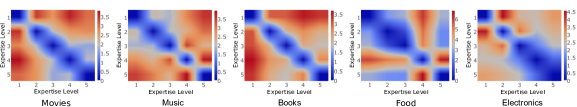
(a) Our model: Facet preference divergence with expertise learned from review helpfulness.

(b) Our model: Language model divergence with expertise learned from review helpfulness.

Figure V.3: Facet preference and language model KL divergence with expertise.

Qualitative Comparison

Log-likelihood of data and convergence: The inference of our model is quite involved with the coupling between several variables, and the alternate stochastic optimization process. Figure V.2 shows the increase in the data log-likelihood of our model per-iteration for each of the five datasets. We observe that the model is stable, and achieves a near smooth increase in the data log-likelihood per-iteration. It also converges quite fast between $20-30$ iterations depending on the complexity of the dataset. For electronics the convergence is quite rapid as the data is quite sparse, and the model does not find sufficient evidence for categorizing users to different expertise levels; this behavior is reflected in all the experiments involving the electronics dataset.

Language model and facet preference divergence: From our initial hypothesis of the joint interaction between review helpfulness, reviewer expertise, facet preferences, and writing style: we expect users at different expertise levels to have divergent facet preferences and Language Models (LM’s) — with expert users having a more sophisticated writing style and vocabulary than amateurs.

Figures V.3(a) and V.3(b) show the heatmaps of the Kullback-Leibler (KL) divergence for facet preferences and language models of users at different expertise levels, as computed by our model conditioned on review helpfulness — given by $D_{KL}(\theta_{e_{i}}||\theta_{e_{j}})$ and $D_{KL}(\phi_{e_{i}}||\phi_{e_{j}})$ respectively, where $\Theta$ and $\Phi$ are given by Equations V.4 and V.9, respectively.

The main observation is that the KL divergence is higher — the larger the difference is between the expertise levels of two users. This confirms our hypothesis. We also note that the increase in divergence with the increase in gap between expertise levels is not smooth for food and electronics — due to the sparsity of per-user data.

Interpretable explanation by salient words used by experts for helpful reviews: Table V.5 shows a snapshot of the latent word clusters, as used by experts and amateurs, for helpful reviews and otherwise, as generated by our model. Once the model parameters are estimated, for each dataset, we consider the expertise-facet pairs $\{e^{+},z^{+}\}$ and $\{e^{-},z^{-}\}$ for which the learned feature weights $\langle\psi_{e,z}\rangle$ are maximum and minimum, respectively. Now, given the language model $\Phi$, we rank the top words from $\phi_{e^{+},z^{+}}$ and $\phi_{e^{-},z^{-}}$ as the words contributing most to helpful reviews, and least helpful reviews, respectively.

We observe that the most helpful reviews pertaining to music talk about the essence and style of music; for books they describe the theme and writing style; for movies they write about screenplay and storytelling; for electronics they discuss about specific product features — note that earlier works [Liu 2008, Kim 2006] used explicit product descriptions as features, that we were able to automatically discover as latent features from textual reviews; whereas for food reviews these are mostly concerned about hygiene and allergens. The least helpful reviews mostly describe some generic concepts in the domain, praise or criticize an item without going in depth about the facets, and are generally quite superficial in nature.

Top words used by experts in most helpful reviews.
Music: album, lyrics, recommend, soundtrack, touch, songwriting, features, rare, musical, ears, lyrical, enjoy, absolutely, musically, individual, bland, soothing, released, inspiration, share, mainstream, deeper, flawless, wonderfully, eclectic, heavily, critics, presence, popularity, brilliantly, inventive
Books: serious, complex, claims, content, illustrations, picture, genre, beautifully, literary, witty, critics, complicated, argument, premise, scholarship, talented, divine, twists, exceptional, obsession, commentary, landscape, exposes, influenced, accomplished, oriented, exploration, styles, storytelling
Movies: scene, recommend, screenplay, business, depth, justice, humanity, packaging, perfection, flicks, sequels, propaganda, anamorphic, cliche&acute, pretentious, goofy, ancient, marvelous, perspective, outrageous, intensity, mildly, immensely, bland, subplots, anticipation, rendered, atrocious
Electronics: adapter, wireless, computer, sounds, camera, range, drives, mounted, photos, shots, packaging, antenna, ease, careful, broken, cards, distortion, stick, media, application, worthless, clarity, technical, memory, steady, dock, items, cord, systems, amps, skin, watt, monitors, arms, pointed
Food: expensive, machine, months, clean, chips, texture, spicy, odor, inside, processed, robust, packs, weather, sticking, alot, press, poured, swallow, reasonably, portions, beware, fragrance, basket, volume, sweetness, terribly, caused, scratching, serves, sensation, sipping, smelled, italian, sensitive, suffered
Top words used by amateurs in least helpful reviews.
Music: will, good, favorite, cool, great, genius, earlier, notes, attention, place, putting, superb, style, room, beauty, realize, brought, passionate, difference, god, fresh, save, musical, grooves, consists, tapes, depressing, interview, short, rock, appeared, learn, brothers, considering, pitched, badly, adding, kiss
Books: will, book, time, religious, liberal, material, interest, utterly, moves, movie, consistent, false, committed, question, turn, coverage, decade, novel, understood, worst, leader, history, kind, energy, fit, dropped, current, doubt, fan, books, building, travel, sudden, fails, wanted, ghost, presents, honestly
Movies: movie, hour, gay, dont, close, previous, features, type, months, meaning, wait, boring, absolutely, truth, generation, going, fighting, runs, fantastic, kids, quiet, kill, lost, angles, previews, crafted, teens, help, believes, brilliance, touches, sea, hardcore, continue, album, formula, listed, drink, text
Electronics: order, attach, replaced, write, impressed, install, learn, tool, offered, details, turns, snap, price, digital, well, buds, fit, problems, photos, hear, shoot, surprisingly, continue, house, card, sports, writing, include, adequate, nice, programming, protected, mistake, response, situations, effects
Food: night, going, haven, sour, fat, avoid, sugar, coffee, store, bodied, graham, variety, salsa, reasons, favorite, delicate, purpose, brands, worst, litter, funny, partially, sesame, handle, excited, close, awful, happily, fully, fits, effects, virgin, salt, returned, powdery, meals, matcha, great, bites, table, pistachios

Table V.5: Snapshot of latent word clusters as used by experts and amateurs for most and least helpful reviews in different domains.

V.4 Finding Credible Reviews with Limited Information using Consistency Features

V.4.1 Review Credibility Analysis

Unlike prior works — in opinion spam and fake review detection — leveraging crude user behavioral and shallow textual features of reviews for credibility classification, we delve deep into the semantics of the reviews to under the inconsistencies that can be used to explain why the review is non-credible, or otherwise using (latent) facet models.

Facet Model

Given review snippets like “the hotel offers free wi-fi”, we now aim to find the different facets present in the reviews along with their corresponding sentiment polarities. Since the aim of this work is to present a model requiring limited prior information, we extract the latent facets from the review text, without the help of any explicit facet or seed words. The ideal machinery should map “wi-fi” to a latent facet cluster like “network, Internet, computer, access, …”. We also want to extract the sentiment expressed in the review about the facet. Interestingly, although “free” does not have a polarity of its own, in the above example “free” in conjunction with “wi-fi” expresses a positive sentiment of a service being offered without charge. The hope is that although “free” does not have an individual polarity, it appears in the neighborhood of words that have known polarities (from lexicons). This helps in the joint discovery of facets and sentiment labels, as “free wi-fi” and “internet without extra charge” should ideally map to the same facet cluster with similar polarities using their co-occurrence with similar words with positive polarities. In this work, we use the Joint Sentiment Topic Model approach (JST) [Lin 2009] to jointly discover the latent facets along with their expressed polarities.

Consider a set of reviews $\langle D\rangle$ written by users $\langle U\rangle$ on a set of items $\langle I\rangle$, with $r_{d}\in R$ being the rating assigned to review $d\in D$. Each review document $d$ consists of a sequence of words $N_{d}$ denoted by $\{w_{1},w_{2},...w_{N_{d}}\}$, and each word is drawn from a vocabulary $V$ indexed by $1,2,..V$. Consider a set of facet assignments $z=\{z_{1},z_{2},...z_{K}\}$ and sentiment label assignments $l=\{l_{1},l_{2},...l_{L}\}$ for $d$, where each $z_{i}$ can be from a set of $K$ possible facets, and each label $l_{i}$ is from a set of $L$ possible sentiment labels.

JST adds a layer of sentiment in addition to the topics as in standard LDA [Blei 2001]. It assumes each document $d$ to be associated with a multinomial distribution $\theta_{d}$ over facets $z$ and sentiment labels $l$ with a symmetric Dirichlet prior $\alpha$. $\theta_{d}(z,l)$ denotes the probability of occurrence of facet $z$ with polarity $l$ in document $d$. Topics have a multinomial distribution $\phi_{z,l}$ over words drawn from a vocabulary $V$ with a symmetric Dirichlet prior $\beta$. $\phi_{z,l}(w)$ denotes the probability of the word $w$ belonging to the facet $z$ with polarity $l$. In the generative process, a sentiment label $l$ is first chosen from a document-specific rating distribution $\pi_{d}$ with a symmetric Dirichlet prior $\gamma$ . Thereafter, one chooses a facet $z$ from $\theta_{d}$ conditioned on $l$, and subsequently a word $w$ from $\phi$ conditioned on $z$ and $l$. Algorithm 4 outlines the generative process. Exact inference is not possible due to intractable coupling between $\Theta$ and $\Phi$, and thus we use Collapsed Gibbs Sampling for approximate inference.

Let $n(d,z,l,w)$ denote the count of the word $w$ occurring in document $d$ belonging to the facet $z$ with polarity $l$. The conditional distribution for the latent variable $z$ (with components $z_{1}$ to $z_{K}$) and $l$ (with components $l_{1}$ to $l_{L}$) is given by:

$$P(z_{i}=k,l_{i}=j| w_{i}=w,z_{-i},l_{-i},w_{-i})\propto$$ (V.11)

$$\frac{n(d,k,j,.)+\alpha}{\sum_{k}n(d,k,j,.)+K\alpha} \times\frac{n(.,k,j,w)+\beta}{\sum_{w}n(.,k,j,w)+V\beta}\times\frac{n(d,.,j,.)+\gamma}{\sum_{j}n(d,.,j,.)+L\gamma}$$

In the above equation, the operator $(.)$ in the count indicates marginalization, i.e., summing up the counts over all values for the corresponding position in $n(d,z,l,w)$, and the subscript $-i$ denotes the value of a variable excluding the data at the $i^{th}$ position.

for each document $d$ do

      choose a distribution $\pi_{d}\sim Dir(\gamma)$

end for

for each sentiment label $l$ under document $d$ do

      choose a distribution $\theta_{d,l}\sim Dir(\alpha)$

end for

for each word $w_{i}$ in document $d$ do

       Choose a sentiment label $l_{i}\sim\pi_{d}$

       Choose a topic $z_{i}\sim\theta_{d,l_{i}}$

       Choose a word $w_{i}$ from the distribution over words $\phi_{l_{i},z_{i}}$

      

end for

Algorithm 4 Joint sentiment topic model [Lin 2009].

Consistency Features

We extract the following features from the latent facet model enabling us to detect inconsistencies in reviews and ratings of items for credibility analysis.

1. User Review – Facet Description: The facet-label distribution of different items differ; for some items, certain facets (with their polarities) are more important than other dimensions. For instance, the “battery life” and “ease of use” for consumer electronics are more important than “color”; for hotels, certain services are available for free (e.g., wi-fi) which may be charged elsewhere. Similarly, user reviews involving less relevant facets of the item under discussion, e.g., downrating hotels for “not allowing pets” should also be detected.

Given a review $d(i)$ on an item $i\in I$ with a sequence of words $\{w\}$ and previously learned $\Phi$, its facet label distribution $\Phi^{{}^{\prime}}_{d}(i)$ with dimension $K\times L$ is given by:

$$\phi^{{}^{\prime}}_{k,l}=\sum_{w:l^{*}=argmax_{l}\ \phi_{k,l}(w)}\phi_{k,l^{*}}(w)$$ (V.12)

For each word $w$ and each latent facet dimension $k$, we consider the sentiment label $l^{*}$ that maximizes the facet-label-word distribution $\phi_{k,l}(w)$, and aggregate this over all the words. This facet-label distribution of the review $\Phi^{{}^{\prime}}_{d}(i)$ of dimension $K\times L$ is used as a feature vector to a classifier to figure out the importance of the different latent dimensions that also captures domain-specific facet-label importance.

2. User Review — Rating: The rating assigned by a user to an item should be consistent to her opinion expressed in the review about the item. For instance, it is unlikely that the user will assign an average or poor rating to an item when she has expressed positive opinion about all the important facets of the item in the review. The inferred rating distribution $\pi^{{}^{\prime}}_{d}$ (with dimension $L$) of a review $d$ consisting of a sequence of words $\{w\}$ and learned $\Phi$ is computed as:

$$\pi^{{}^{\prime}}_{l}=\sum_{w,k:\{k^{*},l^{*}\}=argmax_{k,l}\ \phi_{k,l}(w)}\phi_{k^{*},l^{*}}(w)$$ (V.13)

For each word, we consider the facet and label that jointly maximizes the facet-label-word distribution, and aggregate over all the words and facets. The absolute deviation (of dimension $L$) between the user-assigned rating $\pi_{d}$, and estimated rating $\pi^{{}^{\prime}}_{d}$ from user text is taken as a component in the overall feature vector.

3. User Rating: Prior works [Ott 2011, Sun 2013, Hu 2012] dealing with opinion spam and fake reviews found that these kinds of reviews tend to express overtly positive or overtly negative opinions. Therefore, we also use $\pi^{{}^{\prime}}_{d}$ as a component of the overall feature vector to detect cues from such extreme ratings.

4. Temporal Burst: This is typically observed in group spamming, where a number of reviews are posted targeting an item in a short span of time. Consider a set of reviews $\{d_{j}\}$ at timepoints $\{t_{j}\}$ posted for a specific item. The temporal burstiness of review $d_{i}$ for the given item is given by $\big{(}\sum_{j,j\neq i}\frac{1}{1+e^{t_{i}-t_{j}}}\big{)}$. Here, exponential decay is used to weigh the temporal proximity of reviews to capture the burst.

5. User Review – Item Description: In general, the description of the facets outlined in a user review about an item should not differ markedly from that of the majority. For instance, if the user review says “internet is charged”, and majority says the “hotel offers free wi-fi” — this presents a possible inconsistency. For the facet model this corresponds to word clusters having the same facet label but different sentiment labels. During experiments, however, we find this feature to play a weak role in the presence of other inconsistency features.

We aggregate the per-review facet distribution $\phi^{{}^{\prime}}_{k,l}$ over all the reviews $d(i)$ on the item $i$ to obtain the facet-label distribution $\Phi^{{}^{\prime\prime}}(i)$ of the item. We use the Jensen-Shannon divergence, a symmetric and smoothed version of the Kullback-Leibler divergence as a feature. This depicts how much the facet-label distribution in the given review diverges from the general opinion of other people about the item.

$$JSD(\Phi^{{}^{\prime}}_{d}(i)\ ||\ \Phi^{{}^{\prime\prime}}(i))=\frac{1}{2}(D(\Phi^{{}^{\prime}}_{d}(i)\ ||\ M)+D(\Phi^{{}^{\prime\prime}}(i)\ ||\ M))$$ (V.14)

where, $M=\frac{1}{2}(\Phi^{{}^{\prime}}_{d}(i)+\Phi^{{}^{\prime\prime}}(i))$, and $D$ represents Kullback-Leibler divergence.

Feature vector construction: For each review $d_{j}$, all the above consistency features are computed, and a facet feature vector $\langle F^{T}(d_{j})\rangle$ of dimension $2+K\times L+2L$ is created for subsequent processing.

Additional Language and Behavioral Features

In addition to the above consistency features, we also use limited language and user behavioral features. We later show during experiments that all these features, in conjunction, perform better than the individual feature classes.

In order to capture the distributional difference in the words of deceptive and authentic reviews, we consider unigram and bigram language features that have been shown to outperform other fine-grained linguistic features using psycholinguistic features (e.g., LIWC lexicon) and Part-of-Speech tags [Ott 2011]. Chapter III.4.1 discusses in-depth the various linguistic features effective for distinguishing credible reviews, from non-credible ones.

Language feature vector construction: Consider a vocabulary $V$ of unique unigrams and bigrams in the corpus (after removing stop words). For each token type $f_{i}\in V$ and each review $d_{j}$, we compute the presence/absence of words, $w_{ij}$, of type $f_{i}$ occurring in $d_{j}$, thus constructing a feature vector $F^{L}(d_{j})=\langle w_{ij}=I({w_{ij}=f_{i}})\leavevmode\nobreak\ /\leavevmode\nobreak\ length(d_{j})\rangle,\forall i$, with $I(.)$ denoting an indicator function (notations used are presented in Table V.6).

Earlier works [Jindal 2007, Jindal 2008, Lim 2010] on review spam show that user-dependent models detecting user-preferences and biases perform well in credibility analysis. However, such information is not always available, especially for newcomers, and not so active users in the community. Besides,  [Liu 2012, Mukherjee 2013a] show that spammers tend to open multiple fake accounts to write reviews for malicious activities — using each of those accounts sparsely to avoid detection. Therefore, instead of relying on extensive user history, we use simple proxies for user activity that are easier to aggregate from the community:

• User Posts: number of posts written by the user in the community.

• Review Length: length of the reviews — longer reviews tend to frequently go off-topic with high emotional digression.

• User Rating Behavior: absolute deviation of the review rating from the mean and median rating of the user to other items, as well as the first three moments of the user rating distribution — capturing the scenario where the user has a typical rating behavior across all items.

• Item Rating Pattern: absolute deviation of the item rating from the mean and median rating obtained from other users captures the extent to which the user disagrees with other users about the item quality; the first three moments of the item rating distribution captures the general item rating pattern.

• User Friends: number of friends of the user.

• User Check-in: if the user checked-in the hotel — first hand experience of the user adds to the review credibility.

• Elite: elite status of the user in the community.

• Review helpfulness: number of helpfulness votes received by the user post — captures the quality of user postings.

Note that user rating behavior and item rating pattern are also captured implicitly using the consistency features in the latent facet model.

Also, note that some of these consistency features are also used in the earlier task on detecting helpful product reviews.

Since our aim is to detect credible reviews in the case of limited information, we further split the above activity or behavioral features into two components: (a) $Activity^{-}$ using features $[1-4]$ that can be straightforward obtained from the tuple $\langle userId,itemId,review,rating\rangle$ and are easily available even for “long-tail” items and newcomers; and (b) $Activity^{+}$ using all the listed features. However the latter requires additional information (features $[5-8]$) that might not always be available, or takes long time to aggregate for new items/users.

Behavioral feature vector construction: For each review $d_{j}$ by user $u_{k}$, we construct a behavioral feature vector $\langle F^{B}(d_{j})\rangle$ using the above features.

V.4.2 Tasks

Credible Review Classification

In the first task, we classify reviews as credible or not. For each review $d_{j}$ by user $u_{k}$, we construct the joint feature vector $F(d_{j})=F^{L}(d_{j})\cup F^{T}(d_{j})\cup F^{B}(d_{j})$, and use Support Vector Machines (SVM) [Cortes 1995] for classification of the reviews.

We use the $L_{2}$ regularized $L_{2}$ loss SVM with dual formulation from the LibLinear package [Fan 2008] with other default parameters. We report classification accuracy with $10$-fold cross-validation on ground-truth from TripAdvisor and Yelp.

Item Ranking and Evaluation Measures

Due to the scarcity of ground-truth data pertaining to review credibility, a more suitable way to evaluate our model is to examine the effect of non-credible reviews on the relative ranking of items in the community. For instance, in case of popular items with large number of reviews, even if a fraction of it were non-credible, its effect would not be so severe as would be on “long-tail” items with fewer reviews.

A simple way to find the “goodness” of an item is to aggregate ratings of all reviews – using which we also obtain a ranking of items. We use our model to filter out non-credible reviews, aggregate ratings of credible reviews, and re-compute the item ranks.

Evaluation Measures – We use the Kendall-Tau Rank Correlation Co-efficient ($\tau$) to find effectiveness of the rankings, against a reference ranking — for instance, the sales rank of items in Amazon. $\tau$ measures the number of concordant and discordant pairs, to find whether the ranks of two elements agree or not based on their scores, out of the total number of combinations possible. Given a set of observations $\{x,y\}$, any pair of observations $(x_{i},y_{i})$ and $(x_{j},y_{j})$, where $i\not=j$, are said to be concordant if either $x_{i}>x_{j}$ and $y_{i}>y_{j}$, or $x_{i}<x_{j}$ and $y_{i}<y_{j}$, and discordant otherwise. If $x_{i}=x_{j}$ or $y_{i}=y_{j}$, the ranks are tied — neither discordant, nor concordant.

We use the Kendall-Tau-B measure ($\tau_{b}$) which allows for rank adjustment. Consider $n_{c}$, $n_{d}$, $t_{x}$, and $t_{y}$ to be the number of concordant, discordant, tied pairs on $x$, and tied pairs on $y$ respectively, whereby Kendall-Tau-B is given by: $\frac{n_{c}-n_{d}}{\sqrt{(n_{c}+n_{d}+t_{x})(n_{c}+n_{d}+t_{y})}}$.

However, this is a conservative estimate as multiple items — typically the top-selling ones in Amazon — have the same rating (say, $5$). Therefore, we use a second estimate (say, Kendall-Tau-M ($\tau_{m}$)) which considers non-zero tied ranks to be concordant. Note that, an item can have a zero-rank if all of its reviews are classified as non-credible. A high positive (or, negative) value of Kendall-Tau indicates the two series are positively (or, negatively) correlated; whereas a value close to zero indicates they are independent.

Domain Transfer from Yelp to Amazon

A typical issue in credibility analysis task is the scarcity of labeled training data. In the first task, we use labels from the Yelp Spam Filter (considered to be the industry standard) to train our model. However, such ground-truth labels are not available in Amazon. Although, in principle, we can train a model $M_{\text{Yelp}}$ on Yelp, and use it to filter out non-credible reviews in Amazon.

Transferring the learned model from Yelp to Amazon (or other domains) entails using the learned weights of features in Yelp that are analogous to the ones in Amazon. However, this process encounters the following issues:

• Facet distribution of Yelp (food and restaurants) is different from that of Amazon (products such as software, and consumer electronics). Therefore, the facet-label distribution and the corresponding learned feature weights from Yelp cannot be directly used, as the latent dimensions are different.

• Additionally, specific metadata like check-in, user-friends, and elite-status are missing in Amazon.

However, the learned weights for the following features can still be directly used:

• Certain unigrams and bigrams, especially those depicting opinion, that occur in both domains.

• Behavioral features like user and item rating patterns, review count and length, and usefulness votes.

• Deviation features derived from Amazon-specific facet-label distribution that is obtained using the JST model on Amazon corpus:

  • Deviation (with dimension $L$) of the user assigned rating from that inferred from review content.

  • Distribution (with dimension $L$) of positive and negative sentiment as expressed in the review.

  • Divergence, as a unary feature, of the facet-label distribution in the review from the aggregated distribution over other reviews on a given item.

  • Burstiness, as a unary feature, of the review.

Using the above components, that are common to both Yelp and Amazon, we first re-train the model $M_{\text{Yelp}}$ from Yelp to remove the non-contributing features for Amazon.

Now, a direct transfer of the model weights from Yelp to Amazon assumes the distribution of credible to non-credible reviews, and corresponding feature importance, to be the same in both domains — which is not necessarily true. In order to boost certain features to better identify non-credible reviews in Amazon, we tune the soft margin parameter $C$ in the SVM. $C^{+}$ and $C^{-}$ are regularization parameters for positive and negative class (credible and deceptive), respectively. We use C-SVM [Chen 2004], with slack variables, that optimizes:

$$min_{\vec{w},b,\xi_{i}\geq 0}\frac{1}{2}\vec{w}^{T}\vec{w}+C^{+}\sum_{y_{i}=+1}\xi_{i}+C^{-}\sum_{y_{i}=-1}\xi_{i}$$

$$\text{subject\ to}\ \forall\{(\vec{x_{i}},y_{i})\},y_{i}(\vec{w}^{T}\vec{x}_{i}+b)\geq 1-\xi_{i}$$

The parameters $\{C\}$ provide a trade off as to how wide the margin can be made by moving around certain points which incurs a penalty of $\{C\xi_{i}\}$. A high value of $C^{-}$, for instance, places a large penalty for mis-classifying instances from the negative class, and therefore boosts certain features from that class. As the value of $C^{-}$ increases, the model starts classifying more reviews as non-credible. In the worse case, all the reviews of an item are classified as non-credible, leading to the aggregated item rating being zero.

We use $\tau_{m}$ to find the optimal value of $C^{-}$ by varying it in the interval $C^{-}\in\{0,5,10,15,...150\}$ using a validation set from Amazon as shown in Figure V.4. We observe that as $C^{-}$ increases, $\tau_{m}$ also increases till a certain point as more and more non-credible reviews are filtered out, after which it stabilizes.

Figure V.4: Variation of Kendall-Tau-M ($\tau_{m}$) on different Amazon domains with parameter $C^{-}$ variation (using model $M_{\text{Yelp}}$ trained in Yelp and tested in Amazon).

Notation	Description
$U,D,I$	set of users, reviews, and items resp.
$d,r_{d}$	review text and associated rating
$V,f$	unigrams and bigrams vocab. & token types
$w_{ij}$	word of token type $f_{i}$ in review $d_{j}$
$I(\cdot)$	indicator fn. for presence/absence of words
$z,l$	set of facets and sentiment labels resp.
$K,L$	cardinality of facets and sentiment labels
$\theta_{d}(z,l)$	multinom. prob. distr. of facet $z$
	with sentiment label $l$ in document $d$
$\phi_{z,l}(w)$	multinom. prob. distr. of word $w$ belonging
	to facet $z$ with sentiment label $l$
$\Phi^{\prime},\Phi^{\prime\prime}$	facet-label distr. of review and item resp.
$\alpha,\beta,\gamma$	Dirichlet priors
$\pi,\pi^{\prime}$	review rating distr. & inferred rating distr.
$n(\cdot)$	word count in reviews
$F^{x}(d_{j})$	feature vec. of review $d_{j}$ using lang. (x=L),
	consistency (x=T), and behavior (x=B)
$C^{+},C^{-}$	C-SVM regularization parameters

Table V.6: List of variables and notations used with corresponding description.

Ranking SVM

Our previous approach uses the model $M_{\text{Yelp}}$ trained on Yelp, with the reference ranking (i.e., sales ranking) in Amazon being used only for evaluating the item ranking using the Kendall-Tau measure. As the objective is to obtain a good item ranking based on credible reviews, we can have a model $M_{\text{Amazon}}$ that directly optimizes for Kendall-Tau using the reference ranking as training labels. This allows us to use the entire feature space available in Amazon, including the explicit facet-label distribution and the full vocabulary, which could not be used earlier. The feature space is constructed similarly to that of Yelp.

The goal of Ranking SVM [Joachims 2002] is to learn a ranking function which is concordant with a given ordering of items. The objective is to learn $\vec{w}$ such that $\vec{w}\cdot\vec{x_{i}}>\vec{w}\cdot\vec{x_{j}}$ for most data pairs $\{(\vec{x_{i}},\vec{x_{j}}):y_{i}>y_{j}\in R\}$. Although the problem is known to be NP-hard, it is approximated using SVM techniques with pairwise slack variables $\xi_{i,j}$. The optimization problem is equivalent to that of classifying SVM, but now operating on pairwise difference vectors $(\vec{x_{i}}-\vec{x_{j}})$ with corresponding labels $+1/-1$ indicating which one should be ranked ahead. We use the implementation of [Joachims 2002] that maximizes the empirical Kendall-Tau by minimizing the number of discordant pairs.

Unlike the classification task, where labels are per-review, the ranking task requires labels per-item. Consider $\langle f_{i,j,k}\rangle$ to be the feature vector for the $j^{th}$ review of an item $i$, with $k$ indexing an element of the feature vector. We aggregate these feature vectors element-wise over all the reviews on item $i$ to obtain its feature vector $\langle\frac{\sum_{j}f_{i,j,k}}{\sum_{j}\mathbf{1}}\rangle$.

V.4.3 Experiments

Setup and Data

Parameter initialization: The sentiment lexicon from [Hu 2004] consisting of $2006$ positive and $4783$ negative polarity bearing words is used to initialize the review text based facet-label-word tensor $\Phi$ prior to inference. We consider the number of topics, $K=20$ for Yelp, and $K=50$ for Amazon with the review sentiment labels $L=\{+1,-1\}$ (corresponding to positive and negative rated reviews) initialized randomly.

The symmetric Dirichlet priors are set to $\alpha=50/K$, $\beta=0.01$, and $\gamma=0.1$.

Datasets and Ground-Truth: In this work, we consider the following datasets (refer to Table V.7 and V.8) with available ground-truth information.

Dataset	Non-Credible Reviews	Credible Reviews	Items	Users
TripAdvisor	800	800	20	-
Yelp	5169	37,500	273	24,769
Yelp∗	5169	5169	151	7898

Table V.7: Dataset statistics for review classification (Yelp^∗ denotes balanced dataset using random sampling).

Domain	#Users	#Reviews	#Items with reviews per-item
			$\leq$5	$\leq$10	$\leq$20	$\leq$30	$\leq$40	$\leq$50	Total
Electronics	94,664	121,234	14,797	16,963	18,350	18,829	19,053	19,187	19,518
Software	21,825	26,767	3,814	4,354	4,668	4,767	4,807	4,828	4,889
Sports	656	695	202	226	233	235	235	235	235

Table V.8: Amazon dataset statistics for item ranking, with cumulative #items and varying #reviews.

$\bullet$ The TripAdvisor Dataset [Ott 2011, Ott 2013] contains reviews on $20$ most popular Chicago hotels. The data consists of $1600$ reviews with positive ($5$ star) and negative ($1$ star) sentiment, with $20$ credible and $20$ non-credible reviews on each of the hotels. The authors crawled the credible reviews from online review portals like TripAdvisor; whereas the non-credible ones were generated by users in Amazon Mechanical Turk. The dataset has only the review text and sentiment label (positive/negative ratings) with corresponding hotel names, with no other information on users or items.

$\bullet$ The Yelp Dataset contains reviews on $273$ restaurants in Chicago. The data consists of $37.5K$ recommended (i.e., credible) reviews, and $5K$ non-recommended (i.e., non-credible) reviews given by the Yelp filtering algorithm. The annotated labels (recommended, or not-recommended) for the reviews by the Yelp filter are considered as ground-truth in our work. [Mukherjee 2013b] found that the Yelp spam filter primarily relies on linguistic, behavioral, and social networking features. Additionally, we extract the following information for each review: $\langle userId,itemId$ $,timestamp,rating,review,metadata\rangle$. The meta-data consists of some user activity information as outlined in Section V.4.1.

$\bullet$ The Amazon Dataset used in [Jindal 2008] consists of around $149K$ reviews from $117K$ users on $25K$ items from three domains, namely, Consumer Electronics, Software, and Sports. For each review, we gather the same information tuple as that from Yelp. However, the metadata in this dataset is not as rich as in Yelp, consisting only of helpfulness votes of the reviews.

Further, there exists no explicit ground-truth characterizing the reviews as credible or deceptive in Amazon. To this end, we re-rank the items using our approaches, filtering out possible deceptive reviews (based on the feature vectors), and then compare the ranking to the item sales rank considered as the pseudo ground-truth.

Baselines

We use the following state-of-the-art baselines (given the full set of features that fit with their model) for comparison with our proposed model.

(1) Language Model Baselines: We consider the unigram and bigram language model baselines from [Ott 2011, Ott 2013] that have been shown to outperform other baselines using psycholinguistic features, part-of-speech tags, information gain, etc. We take the best baseline from their work which is a combination of unigrams and bigrams. Our proposed model (N-gram+Facet) enriches it by using length normalization, presence or absence of features, latent facets, etc. The recently proposed doc-to-vec model based on Neural Networks, overcomes the weakness of bag-of-words models by taking the context of words into account, and learns a dense vector representation for each document [Le 2014]. We train the doc-to-vec model in our dataset as a baseline model. In addition, we also consider readability (ARI) and review sentiment scores [Hu 2012] under the hypothesis that writing styles would be random because of diverse customer background. ARI measures the reader’s ability to comprehend a text and is measured as a function of the total number of characters, words, and sentences present, while review sentiment tries to capture the fraction of occurrences of positive/negative sentiment words to the total number of such words used.

(2) Activity & Rating Baselines: We extract all activity, rating and behavioral features of users as proposed in [Jindal 2007, Jindal 2008, Lim 2010, Wang 2011a, Liu 2012, Mukherjee 2013a, Mukherjee 2013b, Li 2014a] from the tuple $\langle userId,itemId,rating,review,$ $metadata\rangle$ in the Yelp dataset. Specifically, we utilize the number of helpful feedbacks, review title length, review rating, use of brand names, percent of positive and negative sentiments, average rating, and rating deviation as features for classification. Further, based on the recent work of [Rahman 2015], we also use the user check-in and user elite status information as additional features for comparison.

Quantitative Analysis

Our experimental setup considers the following evaluations:

(1) Credible review classification: We study the performance of the various approaches in distinguishing a credible review from a non-credible one. Since this forms a binary classification task, we consider a balanced dataset containing equal proportion of data from each of the two classes. On the Yelp dataset, for each item we randomly sample an equal number of credible and non-credible reviews (to obtain Yelp^∗); while the TripAdvisor dataset is already balanced. Table V.9 shows the $10$-fold cross validation accuracy results for the different models on the two datasets. We observe that our proposed consistency and behavioral features exhibit around $15\%$ improvement in Yelp^∗ for classification accuracy over the best performing baselines (refer to Table V.9). Since the TripAdvisor dataset has only review text, the user/activity models could not be used there. This experiment could not be performed on Amazon as well, as the ground-truth for credibility labels of reviews is absent.

Models	Features	TripAdvisor	Yelp∗
Deep Learning	Doc2Vec	69.56	64.84
	Doc2Vec + ARI + Sentiment	76.62	65.01
Activity & Rating	Activity+Rating	-	74.68
	Activity+Rating+Elite+Check-in	-	79.43
Language	Unigram + Bigram	88.37	73.63
	Consistency	80.12	76.5
Behavioral	Activity Model-	-	80.24
	Activity Model+	-	86.35
Aggregated	N-gram + Consistency	89.25	79.72
	N-gram + Activity-	-	82.84
	N-gram + Activity+	-	88.44
	N-gram + Consistency + Activity-	-	86.58
	N-gram + Consistency + Activity+	-	91.09
	$M_{\text{Yelp}}$	-	89.87

Table V.9: Credible review classification accuracy with $10$-fold cross validation. TripAdvisor dataset contains only review texts and no user/activity information.

(2) Item Ranking: In this task we examine the effect of non-credible reviews on the ranking of items in the community. This experiment is performed only on Amazon using the item sales rank as ground or reference ranking, as Yelp does not provide such item rankings. The sales rank provides an indication as to how well a product is selling on Amazon.com and highlights the item’s rank in the corresponding category.

The baseline for the item ranking is based on the aggregated rating of all reviews on an item. The first model $M_{\text{Yelp}}$ (C-SVM) trained on Yelp filters out the non-credible reviews, before aggregating review ratings on an item. The second model $M_{\text{Amazon}}$ (SVM-Rank) is trained on Amazon using SVM-Rank with the reference ranking as training labels. $10$-fold cross-validation results are reported on the two measures of Kendall-Tau ($\tau_{b}$ and $\tau_{m}$) in Table V.10 with respect to the reference ranking. $\tau_{b}$ and $\tau_{m}$ for SVM-Rank are the same since there are no ties. Our first model performs substantially better than the baseline, which, in turn, is outperformed by our second model.

In order to find the effectiveness of our approach in dealing with “long-tail” items, we perform an additional experiment with our best performing model i.e., $M_{\text{Amazon}}$ (SVM-Rank).

We use the model to find Kendall-Tau-M ($\tau_{m}$) rank correlation (with the reference ranking) of items having less than (or equal to) $5,10,20,30,40,$ and $50$ reviews in different domains in Amazon (results reported in Table V.11 with $10$-fold cross validation). We observe that our model performs substantially well even with items having as few as five reviews, with the performance progressively getting better with more reviews per-item.

Domain	Kendall-Tau-B ($\tau_{b}$)		Kendall-Tau-M ($\tau_{m}$)		Kendall-Tau ($\tau_{b}=\tau_{m}$)
	Baseline	$M_{\text{Yelp}}$ (C-SVM)	Baseline	$M_{\text{Yelp}}$ (C-SVM)	$M_{\text{Amazon}}$ (SVM-Rank)
CE	0.011	0.109	0.082	0.135	0.329
Software	0.007	0.184	0.088	0.216	0.426
Sports	0.021	0.155	0.102	0.170	0.325

Table V.10:   Kendall-Tau correlation of different models across domains.

Domain	$\tau_{m}$ with #reviews per-item
	$\leq$5	$\leq$10	$\leq$20	$\leq$30	$\leq$40	$\leq$50	Overall
CE	0.218	0.257	0.290	0.304	0.312	0.317	0.329
Software	0.353	0.375	0.401	0.411	0.417	0.419	0.426
Sports	0.273	0.324	0.310	0.325	0.325	0.325	0.325

Table V.11:   Variation of Kendall-Tau-M ($\tau_{m}$) correlation with #reviews with $M_{\text{Amazon}}$ (SVM-Rank).

Credible Reviews

Non-Credible Reviews

not, also, really, just, like, get, perfect, little, good, one, space, pretty, can, everything, come_back, still, us, right, definitely, enough, much, super, free, around, delicious, no, fresh, big, favorite, lot, selection, sure, friendly, way, dish, since, huge, etc, menu, large, easy, last, room, guests, find, location, time, probably, helpful, great, now, something, two, nice, small, better, sweet, though, loved, happy, love, anything, actually, home

dirty, mediocre, charged, customer_service, signature_lounge, view_city, nice_place, hotel_staff, good_service, never_go, overpriced, several_times, wait_staff, signature_room, outstanding, establishment, architecture_foundation, will_not, long, waste, food_great, glamour_closet, glamour, food_service, love_place, terrible, great_place, wonderful, atmosphere, bill, will_never, good_food, management, great_food, money, worst, horrible, manager, service, rude

Table V.12:   Top n-grams (by feature weights) for credibility classification.

Qualitative Analysis

Language Model: The bigram language model performs very well (refer to Table V.9) on the TripAdvisor dataset due to its artificial creation. Workers in Amazon Mechanical Turk were asked to study all the hotel amenities in their websites, and then write fake reviews about them. As a result, the reviews closely follow the actual hotel descriptions, and, therefore it is quite difficult for the facet model to find contradictions or mismatch in facet descriptions. Consequently, the facet model gives marginal improvement when combined with the language model.

However, the bigram language model and doc-to-vec do not perform so well on the real-world, and naturally noisy Yelp dataset, as they do in the previous one. The facet model also does not perform well in isolation. However, all the components put together give significant performance improvement over the ones in isolation (around $8\%$).

Incorporating writing style using ARI and sentiment measures improves performance of doc-to-vec in the TripAdvisor dataset. However, the improvements are not significant in the real-world Yelp data.

We rank all the features in the joint model for credibility classification by their weights — as given by the C-SVM — and show a snapshot of the top unigrams and bigrams in Table V.12. We observe that credible reviews mostly contain a mix of function and content words, balanced opinions, and a lot of informative unigrams. Non-credible reviews, on the other hand, contain extreme opinions, less function words, and more of sophisticated content words, like, a lot of signature bigrams, to catch the readers’ attention.

Behavioral Model: We find the activity based model to perform the best in isolation (refer to Table V.9). Combined with language and consistency features, the joint model exhibits around $5\%$ improvement in performance. Additional meta-data like the user elite and check-in status improves the performance of activity based baselines, which are not typically available for newcomers in the community. Our model using limited information (N-gram+Consistency+Activity^-) performs better than the activity baselines using fine-grained information about items (like brand description) and user history. Incorporating additional user features (Activity⁺) further boosts its performance.

Consistency Features: We perform ablation tests (refer to Table V.9) to find the effectiveness of the facet based consistency features. We remove the consistency model from the aggregated model, and see significant performance degradation of $3-4\%$ for the Yelp^∗ dataset. In the TripAdvisor dataset the performance reduction is less compared to Yelp due to reasons outlined before.

Table V.13 shows a snapshot of the non-credible reviews, with corresponding (in)consistency features in Yelp and Amazon. We observe inconsistencies like: ratings of deceptive reviews not corroborating with the textual description, irrelevant facets influencing the rating of the target item, contradictions between users, expressing extreme opinions without explanation, depicting temporal “burst” in ratings, etc. In principle, these features can also be used to detect other anomalous phenomena like group-spamming (one of the principal indicators of which is temporal burst), which is out of scope of this work.

Ranking Task: For the ranking task in Amazon (refer to Table V.10), the first model $M_{\text{Yelp}}$ — trained on Yelp and tested on Amazon using C-SVM — performs much better than the baseline exploiting various consistency features. The second model $M_{\text{Amazon}}$ — trained on Amazon using SVM-Rank — outperforms the former exploiting the power of the entire feature space and domain-specific proxy labels unavailable to the former.

“Long-Tail” Items: Table V.11 shows the gradual degradation in performance of the second model $M_{\text{Amazon}}$ (SVM-Rank) in dealing with items with lesser number of reviews. Nevertheless, we observe it to give a substantial Kendall-Tau correlation ($\tau_{m}$) with the reference ranking, with as few as five reviews per-item, demonstrating the effectiveness of our model in dealing with “long-tail” items.

Inconsistency Features	Yelp Review & [Rating]	Amazon Review & [Rating]
user review – rating (promotion/demotion):	never been inside James. never checked in. never visited bar. yet, one of my favorite hotels in Chicago. James has dog friendly area. my dog loves it there. [5]	Excellant product-alarm zone, technical support is almost non-existent because of this i will look to another product. this is unacceptible. [4]
user review – facet description (irrelevant):	you will learn that they are actually EVANGELICAL CHRISTIANS working to proselytize the coffee farmers they buy from. [2]	DO NOT BUY THIS. I used turbo tax since 2003, it never let me down until now. I can’t file because Turbo Tax doesn’t have software updates from the IRS “because of Hurricane Katrina”. [1]
user review – item description (deviation from community):	internet is charged in a $300$ dollar hotel! [3]	The book Amazon offers is a joke! All it provides is the forward which is not written by Kalanithi. I don’t have any sample of HIS writing to know if it appeals. [1]
extreme user rating:	GREAT!!!i give 5 stars!!!Keep it up. [5]	GREAT. This camera takes pictures. [1]
temporal bursts:	Dan’s apartment was beautiful and a great downtown location… (3/14/2012) [5]
	I highly recommend working with Dan and NSRA… (3/14/2012) [5]
	Dan is super friendly, demonstrating that he was confident… (3/14/2012) [5]
	my condo listing with no activity, Dan really stepped in… (4/18/2012) [5]

Table V.13:   Snapshot of non-credible reviews (reproduced verbatim) with inconsistencies.

V.5 Conclusions

In this section, we apply the principles and methods developed earlier for credibility analysis for two tasks in product review communities.

For the first task, we propose an approach to predict helpful product reviews by exploiting the joint interaction between user expertise, writing style, timeliness, and review consistency using Hidden Markov Model – Latent Dirichlet Allocation. Unlike prior works exploiting a variety of syntactic and domain-specific features, our model uses only the information of a user reviewing an item at an explicit timepoint to perform this task — making our approach generalizable across all communities and domains. Additionally, we provide interpretable explanation as to why a review is helpful, in terms of salient words from latent word clusters — that are used by experts to describe important facets of the item under consideration.

Thereafter, for the second task, we harness various (in)consistency features from the latent facet models to analyze (in)consistencies between review description, facets, ratings, and timestamps to find credible product reviews with limited information. Additionally, these features help in providing interpretable explanations as to why a review has been deemed as non-credible.

Our approach works well for “long-tail” items or newcomers in the community with limited prior information / history. We develop multiple models for domain transfer and adaptation, where our model performs very well in the ranking tasks involving “long-tail” items, with as few as five reviews per-item.

We perform extensive experiments on real-world reviews from different domains in Amazon (like books, movies, music, food, and electronics), Yelp and TripAdvisor that demonstrate the effectiveness of our approach over state-of-the-art baselines.

Conclusions

VI.1 Contributions

The first contribution of this dissertation is to develop novel forms of probabilistic graphical models, namely, Conditional Random Fields (CRF), for credibility analysis in online communities. These models jointly leverage the context, structure, and interactions between sources, users, postings, and statements in online communities to ascertain the credibility of user-contributed information. They capture the complex interplay between several factors: the writing style (e.g., subjectivity and rationality, attitude and emotions), (latent) trustworthiness and (latent) expertise of users and sources, (latent) topics of postings, user-user and user-item interactions etc.

We first develop a semi-supervised CRF model for credibility classification of postings and statements that is partially supervised by expert knowledge. We apply this framework to the healthcare domain to extract rare or unobserved side-effects of drugs from user-contributed postings in online healthforums. This is one of the problems where large-scale non-expert data has the potential to complement expert medical knowledge. Furthermore, we develop a continuous CRF model for fine-grained credibility regression in online communities to deal with user-assigned numeric ratings to items. We demonstrate its usefulness for news communities that are plagued with misinformation, bias, and polarization induced by the fairness and style of reporting, and political perspectives of media sources and users. We use the model to jointly identify objective news articles, trustworthy media sources, expert users and their credible postings.

The second contribution deals with the temporal evolution and dynamics of online communities where, users join and leave, adapt to evolving trends, and mature over time. We study this temporal evolution in a collaborative filtering framework to recommend items to users based on their experience or maturity to consume them. To this end, we develop two models for experience evolution of users in online communities. The first one models the users to evolve in a discrete manner employing Hidden Markov Model – Latent Dirichlet Allocation that captures the change in writing style and vocabulary usage with change in users’ (latent) experience level. The second one addresses several drawbacks of this discrete evolution with a natural and continuous evolution model of users’ experience, and their corresponding language model employing Geometric Brownian Motion, Brownian Motion, and Latent Dirichlet Allocation. We, thereafter, develop efficient probabilistic inference techniques using Metropolis Hastings, Kalman Filter, and Gibbs Sampling that are empirically shown to smoothly and continuously increase data log-likelihood over time, as well as have a fast convergence. Experimentally, we show that such experience-aware user models can perform item recommendation better than other state-of-the-art algorithms in communities like beer, movies, food, and news. We also use this model to find useful product reviews that are helpful to the end-users in communities like Amazon.

The third contribution is a method to perform credibility analysis with limited information, especially for “long-tail” items and users with limited history of activity information. We develop methods leveraging latent topic models that analyze inconsistencies between review texts, their ratings and facet descriptions, and temporal bursts to identify non-credible reviews. All these methods for product review communities operate only on the information of a user reviewing an item at an explicit timepoint — making our approach generalizable across all communities and domains. We also propose approaches for domain transfer to deal with missing ground-truth information in one domain, by transferring learned models from other domains.

The fourth contribution deals with providing user-interpretable explanations from probabilistic graphical models that can be used to explain their verdict. To this end, we show (latent) distributional word clusters that demonstrate the usage of words by users with varying experience and trustworthiness, discourse and affective norms of credible vs. non-credible postings, evolution traces of how the users evolve over time and acquire community norms, etc.

VI.2 Outlook

Some future applications and extensions of our model to related tasks are the following.

The proposed models, especially, the ones for product review communities — operating only on user-user, user-item, and item-item interactions — are fairly generic in nature, and easily applicable to other communities and domains. For instance, these can be applied to Question-Answering forums (e.g., Quora) to find reliable and expert answers to queries, and experts one would want to follow for certain topics. These can also be used in other crowdsourcing applications to find reliability of user-contributed information. These models can also be used to analyze inconsistencies between credible and non-credible (i.e. abnormal) behavior to detect anomalies and frauds in networks and systems.

Our proposed continuous Conditional Random Field model — for aggregating information from multiple users and sources (e.g., several weak learners or annotators) taking into account their expertise and interactions — can be used for learning to rank and ensemble learning. For instance, these can be used in Amazon Mechanical Turk to assess annotator reliability, and gold answer for certain query types.

Prior works on Knowledge Base (KB) construction (e.g., Yago [Suchanek 2007], DBpedia [Auer 2007], Freebase [Bollacker 2008]) mostly leverage structured information like Wikipedia infoboxes, category information, etc. Additionally, they also require manual curation to maintain quality and consistency of the KB. Consequently, they have a high precision, but low coverage: whereby, they store information mostly about the prominent entities. On the contrary, crowd-sourced information, being noisy and unstructured, have a high coverage but low precision. To bring these together, our proposed models — specifically, the semi-supervised Conditional Random Field model that learns from partial expert knowledge — can be used to automatically construct KBs (and curate them) from large-scale, structured and unstructured Web content, and structured KBs. Recently, an approach for knowledge fusion using a similar approach has been proposed in [Dong 2014].

Many of the language features for capturing the subjectivity and rationality of information in user postings have been manually identified using bias and affective lexicons, discourse relations, etc. Due to the recent advances in representation learning and deep learning, and correspondence between graphical models and neural networks — a natural extension of our work is to automatically learn these linguistic cues and patterns for credibility analysis from the joint embeddings of context and structure of communities using neural networks.

Most of the prior works on truth-finding and data fusion operate over structured data. Although this dissertation relaxes many of these assumptions, it is mostly geared for online communities with user and item interactions. Therefore, future research should be to address the case of arbitrary textual claims that are expressed freely in an open-domain setting, without making any assumptions on the structure of the claim, or characteristics of the community or website where the claim is made.

References

- [Adler 2007] B. Thomas Adler and Luca de Alfaro. A content-driven reputation system for the wikipedia. In Proceedings of the 16th International Conference on World Wide Web, WWW 2007, Banff, Alberta, Canada, May 8-12, 2007, pages 261–270, 2007.
- [Agarwal 2009] Nitin Agarwal and Huan Liu. Trust in Blogosphere. In Encyclopedia of Database Systems, pages 3187–3191. 2009.
- [Auer 2007] Sören Auer, Christian Bizer, Georgi Kobilarov, Jens Lehmann, Richard Cyganiak and Zachary G. Ives. DBpedia: A Nucleus for a Web of Open Data. In The Semantic Web, 6th International Semantic Web Conference, 2nd Asian Semantic Web Conference, ISWC 2007 + ASWC 2007, Busan, Korea, November 11-15, 2007., pages 722–735, 2007.
- [Baltrusaitis 2014] Tadas Baltrusaitis, Peter Robinson and Louis-Philippe Morency. Continuous Conditional Neural Fields for Structured Regression. In Computer Vision - ECCV 2014 - 13th European Conference, Zurich, Switzerland, September 6-12, 2014, Proceedings, Part IV, pages 593–608, 2014.
- [Björne 2010] Jari Björne, Filip Ginter, Sampo Pyysalo, Jun’ichi Tsujii and Tapio Salakoski. Complex event extraction at PubMed scale. Bioinformatics [ISMB], vol. 26, no. 12, pages 382–390, 2010.
- [Blei 2001] David M. Blei, Andrew Y. Ng and Michael I. Jordan. Latent Dirichlet Allocation. In Advances in Neural Information Processing Systems 14 [Neural Information Processing Systems: Natural and Synthetic, NIPS 2001, December 3-8, 2001, Vancouver, British Columbia, Canada], pages 601–608, 2001.
- [Blei 2006] David M. Blei and John D. Lafferty. Dynamic topic models. In Machine Learning, Proceedings of the Twenty-Third International Conference (ICML 2006), Pittsburgh, Pennsylvania, USA, June 25-29, 2006, pages 113–120, 2006.
- [Blei 2007] David M. Blei and Jon D. McAuliffe. Supervised Topic Models. In Advances in Neural Information Processing Systems 20, Proceedings of the Twenty-First Annual Conference on Neural Information Processing Systems, Vancouver, British Columbia, Canada, December 3-6, 2007, pages 121–128, 2007.
- [Blei 2012] David M. Blei. Probabilistic Topic Models. Communications of the ACM, vol. 55, no. 4, pages 77–84, April 2012.
- [Bohannon 2012] Philip Bohannon, Nilesh N. Dalvi, Yuval Filmus, Nori Jacoby, Sathiya Keerthi and Alok Kirpal. Automatic web-scale information extraction. In Proceedings of the ACM SIGMOD International Conference on Management of Data, SIGMOD 2012, Scottsdale, AZ, USA, May 20-24, 2012, pages 609–612, 2012.
- [Bollacker 2008] Kurt D. Bollacker, Colin Evans, Praveen Paritosh, Tim Sturge and Jamie Taylor. Freebase: a collaboratively created graph database for structuring human knowledge. In Proceedings of the ACM SIGMOD International Conference on Management of Data, SIGMOD 2008, Vancouver, BC, Canada, June 10-12, 2008, pages 1247–1250, 2008.
- [Bundschus 2008] Markus Bundschus, Mathäus Dejori, Martin Stetter, Volker Tresp and Hans-Peter Kriegel. Extraction of semantic biomedical relations from text using conditional random fields. BMC Bioinformatics, vol. 9, 2008.
- [Canini 2011] Kevin Robert Canini, Bongwon Suh and Peter Pirolli. Finding Credible Information Sources in Social Networks Based on Content and Social Structure. In PASSAT/SocialCom 2011, Privacy, Security, Risk and Trust (PASSAT), 2011 IEEE Third International Conference on and 2011 IEEE Third International Conference on Social Computing (SocialCom), Boston, MA, USA, 9-11 Oct., 2011, pages 1–8, 2011.
- [Castillo 2011a] Carlos Castillo, Marcelo Mendoza and Barbara Poblete. Information credibility on twitter. In Proceedings of the 20th International Conference on World Wide Web, WWW 2011, Hyderabad, India, March 28 - April 1, 2011, pages 675–684, 2011.
- [Castillo 2011b] Carlos Castillo, Marcelo Mendoza and Barbara Poblete. Information credibility on twitter. In Proceedings of the 20th International Conference on World Wide Web, WWW 2011, Hyderabad, India, March 28 - April 1, 2011, pages 675–684, 2011.
- [Chen 2004] Di-Rong Chen, Qiang Wu, Yiming Ying and Ding-Xuan Zhou. Support Vector Machine Soft Margin Classifiers: Error Analysis. Journal of Machine Learning Research, vol. 5, pages 1143–1175, 2004.
- [Cline 2001] Rebecca JW Cline and Katie M Haynes. Consumer health information seeking on the Internet: the state of the art. Health education research, vol. 16, no. 6, 2001.
- [Coates 1987] Jennifer Coates. Epistemic Modality and Spoken Discourse. Transactions of the Philological Society, vol. 85, pages 100–131, 1987.
- [Cortes 1995] Corinna Cortes and Vladimir Vapnik. Support-Vector Networks. Machine Learning, vol. 20, no. 3, pages 273–297, 1995.
- [Danescu-Niculescu-Mizil 2013] Cristian Danescu-Niculescu-Mizil, Robert West, Dan Jurafsky, Jure Leskovec and Christopher Potts. No country for old members: user lifecycle and linguistic change in online communities. In 22nd International World Wide Web Conference, WWW ’13, Rio de Janeiro, Brazil, May 13-17, 2013, pages 307–318, 2013.
- [Dave 2003] Kushal Dave, Steve Lawrence and David M. Pennock. Mining the Peanut Gallery: Opinion Extraction and Semantic Classification of Product Reviews. In Proceedings of the 12th International Conference on World Wide Web, WWW ’03, pages 519–528, New York, NY, USA, 2003. ACM.
- [de Alfaro 2011] Luca de Alfaro, Ashutosh Kulshreshtha, Ian Pye and B. Thomas Adler. Reputation systems for open collaboration. Commun. ACM, vol. 54, no. 8, pages 81–87, 2011.
- [Despotovic 2009] Zoran Despotovic. Trust and Reputation in Peer-to-Peer Systems. In Encyclopedia of Database Systems, pages 3183–3187. 2009.
- [Dong 2009] Xin Luna Dong, Laure Berti-Equille and Divesh Srivastava. Integrating Conflicting Data: The Role of Source Dependence. Proceedings of VLDB Endowment, vol. 2, no. 1, pages 550–561, 2009.
- [Dong 2013] Xin Luna Dong and Divesh Srivastava. Compact explanation of data fusion decisions. In 22nd International World Wide Web Conference, WWW ’13, Rio de Janeiro, Brazil, May 13-17, 2013, pages 379–390, 2013.
- [Dong 2014] Xin Dong, Evgeniy Gabrilovich, Geremy Heitz, Wilko Horn, Ni Lao, Kevin Murphy, Thomas Strohmann, Shaohua Sun and Wei Zhang. Knowledge vault: a web-scale approach to probabilistic knowledge fusion. In The 20th ACM SIGKDD International Conference on Knowledge Discovery and Data Mining, KDD ’14, New York, NY, USA - August 24 - 27, 2014, pages 601–610, 2014.
- [Dong 2015] Xin Luna Dong, Evgeniy Gabrilovichet al. Knowledge-based Trust: Estimating the Trustworthiness of Web Sources. Proceedings of VLDB Endowment, vol. 8, no. 9, pages 938–949, May 2015.
- [Drucker 1996] Harris Drucker, Christopher J. C. Burges, Linda Kaufman, Alexander J. Smola and Vladimir Vapnik. Support Vector Regression Machines. In Advances in Neural Information Processing Systems 9, NIPS, Denver, CO, USA, December 2-5, 1996, pages 155–161, 1996.
- [Einhorn 1977] Hillel J. Einhorn, Robin M. Hogarth and Eric Klempner. Quality of group judgment. Psychological Bulletin, 1977.
- [Ernst 2014] Patrick Ernst, Cynthia Meng, Amy Siu and Gerhard Weikum. KnowLife: A knowledge graph for health and life sciences. In IEEE 30th International Conference on Data Engineering, Chicago, ICDE 2014, IL, USA, March 31 - April 4, 2014, pages 1254–1257, 2014.
- [Esuli 2006] Andrea Esuli and Fabrizio Sebastiani. SENTIWORDNET: A Publicly Available Lexical Resource for Opinion Mining. In In Proceedings of the 5th Conference on Language Resources and Evaluation (LREC’06, pages 417–422, 2006.
- [Fan 2008] Rong-En Fan, Kai-Wei Chang, Cho-Jui Hsieh, Xiang-Rui Wang and Chih-Jen Lin. LIBLINEAR: A Library for Large Linear Classification. Journal of Machine Learning Research, vol. 9, pages 1871–1874, 2008.
- [Fang 2014] Hui Fang, Jie Zhang and Nadia Magnenat-Thalmann. Subjectivity grouping: learning from users’ rating behavior. In International conference on Autonomous Agents and Multi-Agent Systems, AAMAS ’14, Paris, France, May 5-9, 2014, pages 1241–1248, 2014.
- [Fei 2013] Geli Fei, Arjun Mukherjee, Bing Liu, Meichun Hsu, Malú Castellanos and Riddhiman Ghosh. Exploiting Burstiness in Reviews for Review Spammer Detection. In Proceedings of the Seventh International Conference on Weblogs and Social Media, ICWSM 2013, Cambridge, Massachusetts, USA, July 8-11, 2013., 2013.
- [Feng 2012] Song Feng, Ritwik Banerjee and Yejin Choi. Syntactic Stylometry for Deception Detection. In The 50th Annual Meeting of the Association for Computational Linguistics, Proceedings of the Conference, July 8-14, 2012, Jeju Island, Korea - Volume 2: Short Papers, pages 171–175, 2012.
- [Fogg 2003] B. J. Fogg. Prominence-interpretation theory: explaining how people assess credibility online. In Extended abstracts of the 2003 Conference on Human Factors in Computing Systems, CHI 2003, Ft. Lauderdale, Florida, USA, April 5-10, 2003, pages 722–723, 2003.
- [Fox 2013] Susannah Fox and Maeve Duggan. Health online 2013. Pew Internet and American Life Project, 2013.
- [Galland 2010] Alban Galland, Serge Abiteboul, Amélie Marian and Pierre Senellart. Corroborating information from disagreeing views. In Proceedings of the Third International Conference on Web Search and Web Data Mining, WSDM 2010, New York, NY, USA, February 4-6, 2010, pages 131–140, 2010.
- [Gallup.com ] Gallup.com. Americans’ Confidence in Newspapers Continues to Erode. http://www.gallup.com/poll/163097/americans-confidence- newspapers-continues-erode.aspx. Accessed: 2015-05-07.
- [Greene 2009] Stephan Greene and Philip Resnik. More than Words: Syntactic Packaging and Implicit Sentiment. In Human Language Technologies: Conference of the North American Chapter of the Association of Computational Linguistics, Proceedings, May 31 - June 5, 2009, Boulder, Colorado, USA, pages 503–511, 2009.
- [Griffiths 2002] Tom Griffiths. Gibbs sampling in the generative model of Latent Dirichlet Allocation. Technical report, 2002.
- [Guha 2004a] Ramanathan V. Guha, Ravi Kumar, Prabhakar Raghavan and Andrew Tomkins. Propagation of trust and distrust. In Proceedings of the 13th international conference on World Wide Web, WWW 2004, New York, NY, USA, May 17-20, 2004, pages 403–412, 2004.
- [Guha 2004b] Ramanathan V. Guha, Ravi Kumar, Prabhakar Raghavan and Andrew Tomkins. Propagation of trust and distrust. In Proceedings of the 13th international conference on World Wide Web, WWW 2004, New York, NY, USA, May 17-20, 2004, pages 403–412, 2004.
- [Günnemann 2014] Stephan Günnemann, Nikou Günnemann and Christos Faloutsos. Detecting anomalies in dynamic rating data: a robust probabilistic model for rating evolution. In The 20th ACM SIGKDD International Conference on Knowledge Discovery and Data Mining, KDD ’14, New York, NY, USA - August 24 - 27, 2014, pages 841–850, 2014.
- [Gupta 2012] Aditi Gupta and Ponnurangam Kumaraguru. Credibility Ranking of Tweets During High Impact Events. In Proceedings of the 1st Workshop on Privacy and Security in Online Social Media, PSOSM ’12, pages 2:2–2:8, New York, NY, USA, 2012. ACM.
- [Gupta 2013] Aditi Gupta, Hemank Lamba, Ponnurangam Kumaraguru and Anupam Joshi. Faking Sandy: characterizing and identifying fake images on Twitter during Hurricane Sandy. In 22nd International World Wide Web Conference, WWW ’13, Rio de Janeiro, Brazil, May 13-17, 2013, Companion Volume, pages 729–736, 2013.
- [Hang 2013] Chung-Wei Hang, Zhe Zhang and Munindar P. Singh. Shin: Generalized Trust Propagation with Limited Evidence. IEEE Computer, vol. 46, no. 3, pages 78–85, 2013.
- [Howard 2011] Philip N. Howard, Aiden Duffy, Deen Freelon, Muzammil Hussain, Will Mari and Marwa Mazaid. Opening Closed Regimes: What Was the Role of Social Media During the Arab Spring? 2011.
- [Hu 2004] Minqing Hu and Bing Liu. Mining and summarizing customer reviews. In Proceedings of the Tenth ACM SIGKDD International Conference on Knowledge Discovery and Data Mining, Seattle, Washington, USA, August 22-25, 2004, pages 168–177, 2004.
- [Hu 2012] Nan Hu, Indranil Bose, Noi Sian Koh and Ling Liu. Manipulation of online reviews: An analysis of ratings, readability, and sentiments. Decision Support Systems, vol. 52, no. 3, pages 674–684, 2012.
- [IMS Institute 2014] Healthcare Informatics IMS Institute. Engaging Patients through Social Media. http://www.theimsinstitute.org/, 2014.
- [Järvelin 2002] Kalervo Järvelin and Jaana Kekäläinen. Cumulated gain-based evaluation of IR techniques. ACM Trans. Inf. Syst., vol. 20, no. 4, pages 422–446, 2002.
- [Jindal 2007] Nitin Jindal and Bing Liu. Analyzing and Detecting Review Spam. In Proceedings of the 7th IEEE International Conference on Data Mining (ICDM 2007), October 28-31, 2007, Omaha, Nebraska, USA, pages 547–552, 2007.
- [Jindal 2008] Nitin Jindal and Bing Liu. Opinion spam and analysis. In Proceedings of the International Conference on Web Search and Web Data Mining, WSDM 2008, Palo Alto, California, USA, February 11-12, 2008, pages 219–230, 2008.
- [Jindal 2013] Prateek Jindal and Dan Roth. End-to-End Coreference Resolution for Clinical Narratives. In IJCAI 2013, Proceedings of the 23rd International Joint Conference on Artificial Intelligence, Beijing, China, August 3-9, 2013, pages 2106–2112, 2013.
- [Joachims 2002] Thorsten Joachims. Optimizing search engines using clickthrough data. In Proceedings of the Eighth ACM SIGKDD International Conference on Knowledge Discovery and Data Mining, July 23-26, 2002, Edmonton, Alberta, Canada, pages 133–142, 2002.
- [Jordan 2002] M.I. Jordan and Y. Weiss. Probabilistic inference in graphical models. Handbook of neural networks and brain theory, 2002.
- [Kalman 1960] R. E. Kalman. A New Approach to Linear Filtering and Prediction Problems. Transactions of the ASME — Journal of Basic Engineering, no. 82 (Series D), pages 35–45, 1960.
- [Kamvar 2003] Sepandar D. Kamvar, Mario T. Schlosser and Hector Garcia-Molina. The Eigentrust algorithm for reputation management in P2P networks. In Proceedings of the Twelfth International World Wide Web Conference, WWW 2003, Budapest, Hungary, May 20-24, 2003, pages 640–651, 2003.
- [Kang 2012] Byungkyu Kang, John O’Donovan and Tobias Höllerer. Modeling topic specific credibility on twitter. In 17th International Conference on Intelligent User Interfaces, IUI ’12, Lisbon, Portugal, February 14-17, 2012, pages 179–188, 2012.
- [Karatzas 1991] Ioannis Karatzas and Steven Eugene Shreve. Brownian motion and stochastic calculus. Graduate texts in mathematics. Springer-Verlag, New York, Berlin, Heidelberg, 1991. Autres tirages corriges : 1996, 1997, 1999, 2000, 2005.
- [Kim 2006] Soo-Min Kim, Patrick Pantel, Timothy Chklovski and Marco Pennacchiotti. Automatically Assessing Review Helpfulness. In EMNLP 2007, Proceedings of the 2006 Conference on Empirical Methods in Natural Language Processing, 22-23 July 2006, Sydney, Australia, pages 423–430, 2006.
- [Koller 2009] Daphne Koller and Nir Friedman. Probabilistic graphical models - principles and techniques. MIT Press, 2009.
- [Koren 2008] Yehuda Koren. Factorization meets the neighborhood: a multifaceted collaborative filtering model. In Proceedings of the 14th ACM SIGKDD International Conference on Knowledge Discovery and Data Mining, Las Vegas, Nevada, USA, August 24-27, 2008, pages 426–434, 2008.
- [Koren 2010] Yehuda Koren. Collaborative filtering with temporal dynamics. Commun. ACM, vol. 53, no. 4, pages 89–97, 2010.
- [Koren 2015] Yehuda Koren and Robert M. Bell. Advances in Collaborative Filtering. In Recommender Systems Handbook, pages 77–118. 2015.
- [Krallinger 2008] Martin Krallinger, Alfonso Valencia and Lynette Hirschman. Linking genes to literature: text mining, information extraction, and retrieval applications for biology. Genome Biology, vol. 9, no. 2, page S8, 2008.
- [Krishnamurthy 2009] Rajasekar Krishnamurthy, Yunyao Li, Sriram Raghavan, Frederick Reiss, Shivakumar Vaithyanathan and Huaiyu Zhu. Web Information Extraction. In Encyclopedia of Database Systems, pages 3473–3478. 2009.
- [Kumar 2016] Srijan Kumar, Robert West and Jure Leskovec. Disinformation on the Web: Impact, Characteristics, and Detection of Wikipedia Hoaxes. In Proceedings of the 25th International Conference on World Wide Web, WWW 2016, Montreal, Canada, April 11 - 15, 2016, pages 591–602, 2016.
- [Kwon 2013] Sejeong Kwon, Meeyoung Cha, Kyomin Jung, Wei Chen and Yajun Wang. Prominent Features of Rumor Propagation in Online Social Media. In 2013 IEEE 13th International Conference on Data Mining, Dallas, TX, USA, December 7-10, 2013, pages 1103–1108, 2013.
- [Lakkaraju 2011] Himabindu Lakkaraju, Chiranjib Bhattacharyya, Indrajit Bhattacharya and Srujana Merugu. Exploiting Coherence for the Simultaneous Discovery of Latent Facets and associated Sentiments. In Proceedings of the Eleventh SIAM International Conference on Data Mining, SDM 2011, April 28-30, 2011, Mesa, Arizona, USA, pages 498–509, 2011.
- [Lampe 2007] Cliff Lampe and R. Kelly Garrett. It’s All News to Me: The Effect of Instruments on Ratings Provision. In 40th Hawaii International International Conference on Systems Science (HICSS-40 2007), CD-ROM / Abstracts Proceedings, 3-6 January 2007, Waikoloa, Big Island, HI, USA, page 180, 2007.
- [Lavergne 2008] Thomas Lavergne, Tanguy Urvoy and François Yvon. Detecting Fake Content with Relative Entropy Scoring. In Proceedings of the ECAI’08 Workshop on Uncovering Plagiarism, Authorship and Social Software Misuse, Patras, Greece, July 22, 2008, 2008.
- [Le 2014] Quoc V. Le and Tomas Mikolov. Distributed Representations of Sentences and Documents. In Proceedings of the 31th International Conference on Machine Learning, ICML 2014, Beijing, China, 21-26 June 2014, pages 1188–1196, 2014.
- [Lewis 2010] Seth C Lewis, Kelly Kaufhold and Dominic L Lasorsa. Thinking about citizen journalism: The philosophical and practical challenges of user-generated content for community newspapers. Journalism Practice, vol. 4, no. 2, 2010.
- [Li 2011] Xian Li, Weiyi Meng and Clement T. Yu. T-verifier: Verifying truthfulness of fact statements. In Proceedings of the 27th International Conference on Data Engineering, ICDE 2011, April 11-16, 2011, Hannover, Germany, pages 63–74, 2011.
- [Li 2012] Xian Li, Xin Luna Dong, Kenneth Lyons, Weiyi Meng and Divesh Srivastava. Truth Finding on the Deep Web: Is the Problem Solved? PVLDB, vol. 6, no. 2, pages 97–108, 2012.
- [Li 2013] Jiwei Li, Myle Ott and Claire Cardie. Identifying Manipulated Offerings on Review Portals. In Proceedings of the 2013 Conference on Empirical Methods in Natural Language Processing, EMNLP 2013, 18-21 October 2013, Grand Hyatt Seattle, Seattle, Washington, USA, A meeting of SIGDAT, a Special Interest Group of the ACL, pages 1933–1942, 2013.
- [Li 2014a] Huayi Li, Zhiyuan Chen, Bing Liu, Xiaokai Wei and Jidong Shao. Spotting Fake Reviews via Collective Positive-Unlabeled Learning. In 2014 IEEE International Conference on Data Mining, ICDM 2014, Shenzhen, China, December 14-17, 2014, pages 899–904, 2014.
- [Li 2014b] Jiwei Li, Myle Ott, Claire Cardie and Eduard H. Hovy. Towards a General Rule for Identifying Deceptive Opinion Spam. In Proceedings of the 52nd Annual Meeting of the Association for Computational Linguistics, ACL 2014, June 22-27, 2014, Baltimore, MD, USA, Volume 1: Long Papers, pages 1566–1576, 2014.
- [Li 2014c] Qi Li, Yaliang Li, Jing Gao, Bo Zhao, Wei Fan and Jiawei Han. Resolving conflicts in heterogeneous data by truth discovery and source reliability estimation. In International Conference on Management of Data, SIGMOD 2014, Snowbird, UT, USA, June 22-27, 2014, pages 1187–1198, 2014.
- [Li 2015a] Huayi Li, Zhiyuan Chen, Arjun Mukherjee, Bing Liu and Jidong Shao. Analyzing and Detecting Opinion Spam on a Large-scale Dataset via Temporal and Spatial Patterns. In Proceedings of the Ninth International Conference on Web and Social Media, ICWSM 2015, University of Oxford, Oxford, UK, May 26-29, 2015, pages 634–637, 2015.
- [Li 2015b] Yaliang Li, Jing Gao, Chuishi Meng, Qi Li, Lu Su, Bo Zhao, Wei Fan and Jiawei Han. A Survey on Truth Discovery. SIGKDD Explorations, vol. 17, no. 2, pages 1–16, 2015.
- [Li 2015c] Yaliang Li, Qi Li, Jing Gao, Lu Su, Bo Zhao, Wei Fan and Jiawei Han. On the Discovery of Evolving Truth. In Proceedings of the 21th ACM SIGKDD International Conference on Knowledge Discovery and Data Mining, Sydney, NSW, Australia, August 10-13, 2015, pages 675–684, 2015.
- [Lim 2010] Ee-Peng Lim, Viet-An Nguyen, Nitin Jindal, Bing Liu and Hady Wirawan Lauw. Detecting product review spammers using rating behaviors. In Proceedings of the 19th ACM Conference on Information and Knowledge Management, CIKM 2010, Toronto, Ontario, Canada, October 26-30, 2010, pages 939–948, 2010.
- [Lin 2008] Chih-Jen Lin, Ruby C. Weng and S. Sathiya Keerthi. Trust Region Newton Method for Logistic Regression. Journal of Machine Learning Research, vol. 9, pages 627–650, 2008.
- [Lin 2009] Chenghua Lin and Yulan He. Joint sentiment/topic model for sentiment analysis. In Proceedings of the 18th ACM Conference on Information and Knowledge Management, CIKM 2009, Hong Kong, China, November 2-6, 2009, pages 375–384, 2009.
- [Lin 2011] Chenghua Lin, Yulan He and Richard Everson. Sentence Subjectivity Detection with Weakly-Supervised Learning. In Fifth International Joint Conference on Natural Language Processing, IJCNLP 2011, Chiang Mai, Thailand, November 8-13, 2011, pages 1153–1161, 2011.
- [Liu 2007] Jingjing Liu, Yunbo Cao, Chin-Yew Lin, Yalou Huang and Ming Zhou. Low-Quality Product Review Detection in Opinion Summarization. In EMNLP-CoNLL 2007, Proceedings of the 2007 Joint Conference on Empirical Methods in Natural Language Processing and Computational Natural Language Learning, June 28-30, 2007, Prague, Czech Republic, pages 334–342, 2007.
- [Liu 2008] Yang Liu, Xiangji Huang, Aijun An and Xiaohui Yu. Modeling and Predicting the Helpfulness of Online Reviews. In Proceedings of the 8th IEEE International Conference on Data Mining (ICDM 2008), December 15-19, 2008, Pisa, Italy, pages 443–452, 2008.
- [Liu 2012] Bing Liu. Sentiment analysis and opinion mining. Synthesis Lectures on Human Language Technologies. Morgan & Claypool Publishers, 2012.
- [Lu 2009] Yue Lu, ChengXiang Zhai and Neel Sundaresan. Rated aspect summarization of short comments. In Proceedings of the 18th International Conference on World Wide Web, WWW 2009, Madrid, Spain, April 20-24, 2009, pages 131–140, 2009.
- [Lu 2010] Yue Lu, Panayiotis Tsaparas, Alexandros Ntoulas and Livia Polanyi. Exploiting social context for review quality prediction. In Proceedings of the 19th International Conference on World Wide Web, WWW 2010, Raleigh, North Carolina, USA, April 26-30, 2010, pages 691–700, 2010.
- [Luca 2015] Michael Luca and Georgios Zervas. Fake It Till You Make It: Reputation, Competition, and Yelp Review Fraud. Technical report, Harvard Business School, 2015.
- [Lukasik 2016] Michal Lukasik, P. K. Srijith, Duy Vu, Kalina Bontcheva, Arkaitz Zubiaga and Trevor Cohn. Hawkes Processes for Continuous Time Sequence Classification: an Application to Rumour Stance Classification in Twitter. In Proceedings of the 54th Annual Meeting of the Association for Computational Linguistics, ACL 2016, August 7-12, 2016, Berlin, Germany, Volume 2: Short Papers, 2016.
- [Ma 2011] Hao Ma, Dengyong Zhou, Chao Liu, Michael R. Lyu and Irwin King. Recommender systems with social regularization. In Proceedings of the Forth International Conference on Web Search and Web Data Mining, WSDM 2011, Hong Kong, China, February 9-12, 2011, pages 287–296, 2011.
- [Ma 2015] Fenglong Ma, Yaliang Li, Qi Li, Minghui Qiu, Jing Gao, Shi Zhi, Lu Su, Bo Zhao, Heng Ji and Jiawei Han. FaitCrowd: Fine Grained Truth Discovery for Crowdsourced Data Aggregation. In Proceedings of the 21th ACM SIGKDD International Conference on Knowledge Discovery and Data Mining, Sydney, NSW, Australia, August 10-13, 2015, pages 745–754, 2015.
- [McAuley 2013a] Julian J. McAuley and Jure Leskovec. Hidden factors and hidden topics: understanding rating dimensions with review text. In Seventh ACM Conference on Recommender Systems, RecSys ’13, Hong Kong, China, October 12-16, 2013, pages 165–172, 2013.
- [McAuley 2013b] Julian John McAuley and Jure Leskovec. From amateurs to connoisseurs: modeling the evolution of user expertise through online reviews. In 22nd International World Wide Web Conference, WWW ’13, Rio de Janeiro, Brazil, May 13-17, 2013, pages 897–908, 2013.
- [McCallum 2005] Andrew McCallum, Kedar Bellare and Fernando C. N. Pereira. A Conditional Random Field for Discriminatively-trained Finite-state String Edit Distance. In UAI ’05, Proceedings of the 21st Conference in Uncertainty in Artificial Intelligence, Edinburgh, Scotland, July 26-29, 2005, pages 388–395, 2005.
- [Mihalcea 2009] Rada Mihalcea and Carlo Strapparava. The Lie Detector: Explorations in the Automatic Recognition of Deceptive Language. In ACL 2009, Proceedings of the 47th Annual Meeting of the Association for Computational Linguistics and the 4th International Joint Conference on Natural Language Processing of the AFNLP, 2-7 August 2009, Singapore, Short Papers, pages 309–312, 2009.
- [Miller 1995] George A. Miller. WordNet: A Lexical Database for English. Communications of the ACM, vol. 38, no. 11, pages 39–41, November 1995.
- [Mimno 2008] David M. Mimno and Andrew McCallum. Topic Models Conditioned on Arbitrary Features with Dirichlet-multinomial Regression. In UAI 2008, Proceedings of the 24th Conference in Uncertainty in Artificial Intelligence, Helsinki, Finland, July 9-12, 2008, pages 411–418, 2008.
- [Mitchell 2016] Amy Mitchell, Jeffrey Gottfried, Michael Barthel and Elisa Shearer. Trust and Accuracy. Pew Internet and American Life Project, 2016.
- [Mudambi 2010] Susan M. Mudambi and David Schuff. What Makes a Helpful Online Review? A Study of Customer Reviews on Amazon.com. MIS Quarterly, vol. 34, no. 1, pages 185–200, 2010.
- [Mukherjee 2012] Subhabrata Mukherjee and Pushpak Bhattacharyya. Sentiment Analysis in Twitter with Lightweight Discourse Analysis. In COLING 2012, 24th International Conference on Computational Linguistics, Proceedings of the Conference: Technical Papers, 8-15 December 2012, Mumbai, India, pages 1847–1864, 2012.
- [Mukherjee 2013a] Arjun Mukherjee, Abhinav Kumar, Bing Liu, Junhui Wang, Meichun Hsu, Malú Castellanos and Riddhiman Ghosh. Spotting opinion spammers using behavioral footprints. In The 19th ACM SIGKDD International Conference on Knowledge Discovery and Data Mining, KDD 2013, Chicago, IL, USA, August 11-14, 2013, pages 632–640, 2013.
- [Mukherjee 2013b] Arjun Mukherjee, Vivek Venkataraman, Bing Liu and Natalie S. Glance. What Yelp Fake Review Filter Might Be Doing? In Proceedings of the Seventh International Conference on Weblogs and Social Media, ICWSM 2013, Cambridge, Massachusetts, USA, July 8-11, 2013., 2013.
- [Mukherjee 2013c] Subhabrata Mukherjee, Gaurab Basu and Sachindra Joshi. Incorporating author preference in sentiment rating prediction of reviews. In 22nd International World Wide Web Conference, WWW ’13, Rio de Janeiro, Brazil, May 13-17, 2013, Companion Volume, pages 47–48, 2013.
- [Mukherjee 2014a] Subhabrata Mukherjee, Gaurab Basu and Sachindra Joshi. Joint Author Sentiment Topic Model. In Proceedings of the 2014 SIAM International Conference on Data Mining, Philadelphia, Pennsylvania, USA, April 24-26, 2014, pages 370–378, 2014.
- [Mukherjee 2014b] Subhabrata Mukherjee, Gerhard Weikum and Cristian Danescu-Niculescu-Mizil. People on drugs: credibility of user statements in health communities. In The 20th ACM SIGKDD International Conference on Knowledge Discovery and Data Mining, KDD ’14, New York, NY, USA - August 24 - 27, 2014, pages 65–74, 2014.
- [Mukherjee 2015a] Subhabrata Mukherjee, Hemank Lamba and Gerhard Weikum. Experience-Aware Item Recommendation in Evolving Review Communities. In 2015 IEEE International Conference on Data Mining, ICDM 2015, Atlantic City, NJ, USA, November 14-17, 2015, pages 925–930, 2015.
- [Mukherjee 2015b] Subhabrata Mukherjee and Gerhard Weikum. Leveraging Joint Interactions for Credibility Analysis in News Communities. In Proceedings of the 24th ACM International on Conference on Information and Knowledge Management, CIKM 2015, Melbourne, VIC, Australia, October 19 - 23, 2015, pages 353–362, 2015.
- [Mukherjee 2016a] Subhabrata Mukherjee, Sourav Dutta and Gerhard Weikum. Credible Review Detection with Limited Information Using Consistency Features. In Machine Learning and Knowledge Discovery in Databases - European Conference, ECML PKDD 2016, Riva del Garda, Italy, September 19-23, 2016, Proceedings, Part II, pages 195–213, 2016.
- [Mukherjee 2016b] Subhabrata Mukherjee, Stephan Günnemann and Gerhard Weikum. Continuous Experience-aware Language Model. In Proceedings of the 22nd ACM SIGKDD International Conference on Knowledge Discovery and Data Mining, San Francisco, CA, USA, August 13-17, 2016, pages 1075–1084, 2016.
- [Mukherjee 2017] Subhabrata Mukherjee, Kashyap Popat and Gerhard Weikum. Exploring Latent Semantic Factors to Find Useful Product Reviews. In Proceedings of the 2017 SIAM International Conference on Data Mining, Houston, Texas, USA, April 27-29, 2017, 2017.
- [Nakashole 2014] Ndapandula Nakashole and Tom M. Mitchell. Language-Aware Truth Assessment of Fact Candidates. In Proceedings of the 52nd Annual Meeting of the Association for Computational Linguistics, ACL 2014, June 22-27, 2014, Baltimore, MD, USA, Volume 1: Long Papers, pages 1009–1019, 2014.
- [Nber.org ] Nber.org. Media Bias and Voting. http://www.nber.org/digest/oct06/w12169.html. Accessed: 2015-05-07.
- [Nielsen ] Corporations Nielsen. Global Online Shopping Report. http://www.nielsen.com/us/en/insights/news/2010/global-online-shopping-report.html. [Online; accessed 10-Jun-2016].
- [Nytimes.com ] Nytimes.com. Should Reddit Be Blamed for the Spreading of a Smear? http://www.nytimes.com/2013/07/28/magazine/should-reddit-be- blamed-for-the-spreading-of-a-smear.html. Accessed: 2015-05-07.
- [O’Mahony 2009] Michael P. O’Mahony and Barry Smyth. Learning to recommend helpful hotel reviews. In Proceedings of the 2009 ACM Conference on Recommender Systems, RecSys 2009, New York, NY, USA, October 23-25, 2009, pages 305–308, 2009.
- [Ott 2011] Myle Ott, Yejin Choi, Claire Cardie and Jeffrey T. Hancock. Finding Deceptive Opinion Spam by Any Stretch of the Imagination. In The 49th Annual Meeting of the Association for Computational Linguistics: Human Language Technologies, Proceedings of the Conference, 19-24 June, 2011, Portland, Oregon, USA, pages 309–319, 2011.
- [Ott 2013] Myle Ott, Claire Cardie and Jeffrey T. Hancock. Negative Deceptive Opinion Spam. In Human Language Technologies: Conference of the North American Chapter of the Association of Computational Linguistics, Proceedings, June 9-14, 2013, Westin Peachtree Plaza Hotel, Atlanta, Georgia, USA, pages 497–501, 2013.
- [Pan 2004] A Sentimental Education: Sentiment Analysis Using Subjectivity Summarization Based on Minimum Cuts. In Proceedings of the 42nd Annual Meeting of the Association for Computational Linguistics, 21-26 July, 2004, Barcelona, Spain., pages 271–278, 2004.
- [Pang 2002] Bo Pang and Vaithyanathan Shivakumar Lee Lillian. Thumbs up?: sentiment classification using machine learning techniques. In Proceedings of the 2002 Conference on Empirical Methods in Natural Language Processing, EMNLP ’02, 2002.
- [Pang 2007] Bo Pang and Lillian Lee. Opinion Mining and Sentiment Analysis. Foundations and Trends in Information Retrieval, vol. 2, no. 1-2, pages 1–135, 2007.
- [Pasternack 2010] Jeff Pasternack and Dan Roth. Knowing What to Believe (when you already know something). In COLING 2010, 23rd International Conference on Computational Linguistics, Proceedings of the Conference, 23-27 August 2010, Beijing, China, pages 877–885, 2010.
- [Pasternack 2011] Jeff Pasternack and Dan Roth. Making Better Informed Trust Decisions with Generalized Fact-Finding. In IJCAI 2011, Proceedings of the 22nd International Joint Conference on Artificial Intelligence, Barcelona, Catalonia, Spain, July 16-22, 2011, pages 2324–2329, 2011.
- [Pasternack 2013] Jeff Pasternack and Dan Roth. Latent credibility analysis. In 22nd International World Wide Web Conference, WWW ’13, Rio de Janeiro, Brazil, May 13-17, 2013, pages 1009–1020, 2013.
- [Paul 2013] Michael J. Paul and Mark Dredze. Drug Extraction from the Web: Summarizing Drug Experiences with Multi-Dimensional Topic Models. In Human Language Technologies: Conference of the North American Chapter of the Association of Computational Linguistics, Proceedings, June 9-14, 2013, Westin Peachtree Plaza Hotel, Atlanta, Georgia, USA, pages 168–178, 2013.
- [Pennebaker 2001] J.W. Pennebaker, M.E. Francis and R.J. Booth. Linguistic inquiry and word count: A computerized text analysis program. Psychology Press, 2001.
- [Peterson 2003] Geraldine Peterson, Parisa Aslani and A. Kylie Williams. How do Consumers Search for and Appraise Information on Medicines on the Internet? A Qualitative Study Using Focus Groups. Journal of Medical Internet Research, vol. 5, no. 4, page e33, Dec 2003.
- [Qazvinian 2011] Vahed Qazvinian, Emily Rosengren, Dragomir R. Radev and Qiaozhu Mei. Rumor has it: Identifying Misinformation in Microblogs. In Proceedings of the 2011 Conference on Empirical Methods in Natural Language Processing, EMNLP 2011, 27-31 July 2011, John McIntyre Conference Centre, Edinburgh, UK, A meeting of SIGDAT, a Special Interest Group of the ACL, pages 1589–1599, 2011.
- [Qin 2008] Tao Qin, Tie-Yan Liu, Xu-Dong Zhang, De-Sheng Wang and Hang Li. Global Ranking Using Continuous Conditional Random Fields. In Advances in Neural Information Processing Systems 21, Proceedings of the Twenty-Second Annual Conference on Neural Information Processing Systems, Vancouver, British Columbia, Canada, December 8-11, 2008, pages 1281–1288, 2008.
- [Radosavljevic 2010] Vladan Radosavljevic, Slobodan Vucetic and Zoran Obradovic. Continuous Conditional Random Fields for Regression in Remote Sensing. In ECAI 2010 - 19th European Conference on Artificial Intelligence, Lisbon, Portugal, August 16-20, 2010, Proceedings, pages 809–814, 2010.
- [Rahman 2015] Mahmudur Rahman, Bogdan Carbunar, Jaime Ballesteros and Duen Horng (Polo) Chau. To catch a fake: Curbing deceptive Yelp ratings and venues. Statistical Analysis and Data Mining, vol. 8, no. 3, pages 147–161, 2015.
- [Ramage 2011] Daniel Ramage, Christopher D. Manning and Susan T. Dumais. Partially labeled topic models for interpretable text mining. In Proceedings of the 17th ACM SIGKDD International Conference on Knowledge Discovery and Data Mining, San Diego, CA, USA, August 21-24, 2011, pages 457–465, 2011.
- [Recasens 2013] Marta Recasens, Cristian Danescu-Niculescu-Mizil and Dan Jurafsky. Linguistic Models for Analyzing and Detecting Biased Language. In Proceedings of the 51st Annual Meeting of the Association for Computational Linguistics, ACL 2013, 4-9 August 2013, Sofia, Bulgaria, Volume 1: Long Papers, pages 1650–1659, 2013.
- [Rosen-Zvi 2004a] Michal Rosen-Zvi, Thomas L. Griffiths, Mark Steyvers and Padhraic Smyth. The Author-Topic Model for Authors and Documents. In UAI ’04, Proceedings of the 20th Conference in Uncertainty in Artificial Intelligence, Banff, Canada, July 7-11, 2004, pages 487–494, 2004.
- [Rosen-Zvi 2004b] Michal Rosen-Zvi, Thomas L. Griffiths, Mark Steyvers and Padhraic Smyth. The Author-Topic Model for Authors and Documents. In UAI ’04, Proceedings of the 20th Conference in Uncertainty in Artificial Intelligence, Banff, Canada, July 7-11, 2004, pages 487–494, 2004.
- [Sarawagi 2008] Sunita Sarawagi. Information Extraction. Foundations and Trends in Databases, vol. 1, no. 3, pages 261–377, 2008.
- [Shayne 2003] Bowman Shayne and Willis Chris. We Media: How Audiences are Shaping the Future of News and Information. 2003.
- [Sloanreview.mit.edu ] Sloanreview.mit.edu. The Problem With Online Ratings. http://sloanreview.mit.edu/article/the-problem-with-online-ratings-2/ . Accessed: 2015-05-07.
- [Snyder 2007] Benjamin Snyder and Regina Barzilay. Multiple Aspect Ranking Using the Good Grief Algorithm. In Human Language Technology Conference of the North American Chapter of the Association of Computational Linguistics, Proceedings, April 22-27, 2007, Rochester, New York, USA, pages 300–307, 2007.
- [Somasundaran 2009] Swapna Somasundaran and Janyce Wiebe. Recognizing Stances in Online Debates. In ACL 2009, Proceedings of the 47th Annual Meeting of the Association for Computational Linguistics and the 4th International Joint Conference on Natural Language Processing of the AFNLP, 2-7 August 2009, Singapore, pages 226–234, 2009.
- [Sridhar ] Dhanya Sridhar, Lise Getoor and Marilyn Walker. Collective Stance Classification of Posts in Online Debate Forums. In ACL Joint Workshop on Social Dynamics and Personal Attributes in Social Media 2014.
- [Strapparava 2004] Carlo Strapparava and Alessandro Valitutti. WordNet Affect: an Affective Extension of WordNet. In Proceedings of the Fourth International Conference on Language Resources and Evaluation, LREC 2004, May 26-28, 2004, Lisbon, Portugal, 2004.
- [Stuart 2007] Allan Stuart. Citizen Journalism and the Rise of ‘Mass Self-Communication’: Reporting the London Bombings. Global Media, vol. 1, no. 1, 2007.
- [Suchanek 2007] Fabian M. Suchanek, Gjergji Kasneci and Gerhard Weikum. Yago: a core of semantic knowledge. In Proceedings of the 16th International Conference on World Wide Web, WWW 2007, Banff, Alberta, Canada, May 8-12, 2007, pages 697–706, 2007.
- [Suchanek 2013] Fabian M. Suchanek and Gerhard Weikum. Knowledge harvesting from text and Web sources. In 29th IEEE International Conference on Data Engineering, ICDE 2013, Brisbane, Australia, April 8-12, 2013, pages 1250–1253, 2013.
- [Sun 2013] Huan Sun, Alex Morales and Xifeng Yan. Synthetic review spamming and defense. In The 19th ACM SIGKDD International Conference on Knowledge Discovery and Data Mining, KDD 2013, Chicago, IL, USA, August 11-14, 2013, pages 1088–1096, 2013.
- [Sutton 2012] Charles A. Sutton and Andrew McCallum. An Introduction to Conditional Random Fields. Foundations and Trends in Machine Learning, vol. 4, no. 4, pages 267–373, 2012.
- [Tang 2013] Jiliang Tang, Huiji Gao, Xia Hu and Huan Liu. Context-aware review helpfulness rating prediction. In Seventh ACM Conference on Recommender Systems, RecSys ’13, Hong Kong, China, October 12-16, 2013, pages 1–8, 2013.
- [Titov 2008] Ivan Titov and Ryan T. McDonald. A Joint Model of Text and Aspect Ratings for Sentiment Summarization. In ACL 2008, Proceedings of the 46th Annual Meeting of the Association for Computational Linguistics, June 15-20, 2008, Columbus, Ohio, USA, pages 308–316, 2008.
- [Turney 2002] Peter D. Turney. Thumbs Up or Thumbs Down?: Semantic Orientation Applied to Unsupervised Classification of Reviews. In Proceedings of the 40th Annual Meeting on Association for Computational Linguistics, ACL ’02, pages 417–424, Stroudsburg, PA, USA, 2002. Association for Computational Linguistics.
- [Vydiswaran 2011a] V. G. Vinod Vydiswaran, ChengXiang Zhai and Dan Roth. Content-driven trust propagation framework. In Proceedings of the 17th ACM SIGKDD International Conference on Knowledge Discovery and Data Mining, San Diego, CA, USA, August 21-24, 2011, pages 974–982, 2011.
- [Vydiswaran 2011b] V.G. Vinod Vydiswaran, ChengXiang Zhai and Dan Roth. Gauging the Internet Doctor: Ranking Medical Claims Based on Community Knowledge. In Proceedings of the 2011 Workshop on Data Mining for Medicine and Healthcare, DMMH ’11, pages 42–51, New York, NY, USA, 2011. ACM.
- [Vydiswaran 2012] V. G. Vinod Vydiswaran, ChengXiang Zhai, Dan Roth and Peter Pirolli. BiasTrust: teaching biased users about controversial topics. In 21st ACM International Conference on Information and Knowledge Management, CIKM’12, Maui, HI, USA, October 29 - November 02, 2012, pages 1905–1909, 2012.
- [Walker 2012] Marilyn A. Walker, Pranav Anand, Rob Abbott and Ricky Grant. Stance Classification using Dialogic Properties of Persuasion. In Human Language Technologies: Conference of the North American Chapter of the Association of Computational Linguistics, Proceedings, June 3-8, 2012, Montréal, Canada, pages 592–596, 2012.
- [Wallach 2009] Hanna M. Wallach, Iain Murray, Ruslan Salakhutdinov and David M. Mimno. Evaluation methods for topic models. In Proceedings of the 26th Annual International Conference on Machine Learning, ICML 2009, Montreal, Quebec, Canada, June 14-18, 2009, pages 1105–1112, 2009.
- [Wang 2006] Xuerui Wang and Andrew McCallum. Topics over time: a non-Markov continuous-time model of topical trends. In Proceedings of the Twelfth ACM SIGKDD International Conference on Knowledge Discovery and Data Mining, Philadelphia, PA, USA, August 20-23, 2006, pages 424–433, 2006.
- [Wang 2010] Hongning Wang, Yue Lu and Chengxiang Zhai. Latent aspect rating analysis on review text data: a rating regression approach. In Proceedings of the 16th ACM SIGKDD International Conference on Knowledge Discovery and Data Mining, Washington, DC, USA, July 25-28, 2010, pages 783–792, 2010.
- [Wang 2011a] Guan Wang, Sihong Xie, Bing Liu and Philip S. Yu. Review Graph Based Online Store Review Spammer Detection. In 11th IEEE International Conference on Data Mining, ICDM 2011, Vancouver, BC, Canada, December 11-14, 2011, pages 1242–1247, 2011.
- [Wang 2011b] Hongning Wang, Yue Lu and ChengXiang Zhai. Latent aspect rating analysis without aspect keyword supervision. In Proceedings of the 17th ACM SIGKDD International Conference on Knowledge Discovery and Data Mining, San Diego, CA, USA, August 21-24, 2011, pages 618–626, 2011.
- [Wang 2012] Chong Wang, David M. Blei and David Heckerman. Continuous Time Dynamic Topic Models. CoRR, vol. abs/1206.3298, 2012.
- [West 2014] Robert West, Hristo S. Paskov, Jure Leskovec and Christopher Potts. Exploiting Social Network Structure for Person-to-Person Sentiment Analysis. TACL, vol. 2, pages 297–310, 2014.
- [Westnet 2009] P. Westnet. HOW TO BE MORE OR LESS CERTAIN IN ENGLISH: SCALARITY IN EPISTEMIC MODALITY. IRAL - International Review of Applied Linguistics in Language Teaching, vol. 24, no. 1-4, pages 311–336, 2009.
- [White 2014a] R W White, R Harpaz, N H Shah, W DuMouchel and E Horvitz. Toward Enhanced Pharmacovigilance Using Patient-Generated Data on the Internet. Clinical Pharmacology & Therapeutics, vol. 96, no. 2, pages 239–246, 2014.
- [White 2014b] Ryen W. White and Eric Horvitz. From health search to healthcare: explorations of intention and utilization via query logs and user surveys. Journal of the American Medical Informatics Association, vol. 21, no. 1, pages 49–55, 2014.
- [Wiebe 2005] Janyce Wiebe and Ellen Riloff. Creating Subjective and Objective Sentence Classifiers from Unannotated Texts. In Computational Linguistics and Intelligent Text Processing, 6th International Conference, CICLing 2005, Mexico City, Mexico, February 13-19, 2005, Proceedings, pages 486–497, 2005.
- [Wiebe 2011] Janyce Wiebe and Ellen Riloff. Finding Mutual Benefit between Subjectivity Analysis and Information Extraction. IEEE Transactions on Affective Computing, vol. 2, no. 4, pages 175–191, 2011.
- [Wolf 2004] Florian Wolf, Edward Gibson and Timothy Desmet. Discourse coherence and pronoun resolution. Language and Cognitive Processes, vol. 19, no. 6, 2004.
- [Xiang 2010] Liang Xiang, Quan Yuan, Shiwan Zhao, Li Chen, Xiatian Zhang, Qing Yang and Jimeng Sun. Temporal recommendation on graphs via long- and short-term preference fusion. In Proceedings of the 16th ACM SIGKDD International Conference on Knowledge Discovery and Data Mining, Washington, DC, USA, July 25-28, 2010, pages 723–732, 2010.
- [Xiong 2010] Liang Xiong, Xi Chen, Tzu-Kuo Huang, Jeff G. Schneider and Jaime G. Carbonell. Temporal Collaborative Filtering with Bayesian Probabilistic Tensor Factorization. In Proceedings of the SIAM International Conference on Data Mining, SDM 2010, April 29 - May 1, 2010, Columbus, Ohio, USA, pages 211–222, 2010.
- [Xu 2012a] Qiongkai Xu and Hai Zhao. Using Deep Linguistic Features for Finding Deceptive Opinion Spam. In COLING 2012, 24th International Conference on Computational Linguistics, Proceedings of the Conference: Posters, 8-15 December 2012, Mumbai, India, pages 1341–1350, 2012.
- [Xu 2012b] Yan Xu, Kai Hong, Junichi Tsujii and Eric I-Chao Chang. Feature engineering combined with machine learning and rule-based methods for structured information extraction from narrative clinical discharge summaries. JAMIA, vol. 19, no. 5, pages 824–832, 2012.
- [Yang 2012] Fan Yang, Yang Liu, Xiaohui Yu and Min Yang. Automatic Detection of Rumor on Sina Weibo. In Proceedings of the ACM SIGKDD Workshop on Mining Data Semantics, MDS ’12, pages 13:1–13:7, New York, NY, USA, 2012. ACM.
- [Yin 2008] Xiaoxin Yin, Jiawei Han and Philip S. Yu. Truth Discovery with Multiple Conflicting Information Providers on the Web. IEEE Transactions on Knowledge and Data Engineering, vol. 20, no. 6, pages 796–808, June 2008.
- [Yoo 2009] Kyung Hyan Yoo and Ulrike Gretzel. Comparison of Deceptive and Truthful Travel Reviews. In Information and Communication Technologies in Tourism, ENTER 2009, Proceedings of the International Conference in Amsterdam, The Netherlands, 2009, pages 37–47, 2009.
- [Yu 2003] Hong Yu and Vasileios Hatzivassiloglou. Towards Answering Opinion Questions: Separating Facts from Opinions and Identifying the Polarity of Opinion Sentences. In Proceedings of the 2003 Conference on Empirical Methods in Natural Language Processing, EMNLP ’03, pages 129–136, Stroudsburg, PA, USA, 2003. Association for Computational Linguistics.
- [Yu 2011] Jianxing Yu, Zheng-Jun Zha, Meng Wang and Tat-Seng Chua. Aspect Ranking: Identifying Important Product Aspects from Online Consumer Reviews. In The 49th Annual Meeting of the Association for Computational Linguistics: Human Language Technologies, Proceedings of the Conference, 19-24 June, 2011, Portland, Oregon, USA, pages 1496–1505, 2011.
- [Zhao 2012a] Bo Zhao and Jiawei Han. A Probabilistic Model for Estimating Real-valued Truth from Conflicting Sources. QDB, 2012.
- [Zhao 2012b] Bo Zhao, Benjamin I. P. Rubinstein, Jim Gemmell and Jiawei Han. A Bayesian Approach to Discovering Truth from Conflicting Sources for Data Integration. Proceedings of VLDB Endowment, vol. 5, no. 6, pages 550–561, 2012.
- [Zhao 2012c] Bo Zhao, Benjamin I. P. Rubinstein, Jim Gemmell and Jiawei Han. A Bayesian Approach to Discovering Truth from Conflicting Sources for Data Integration. PVLDB, vol. 5, no. 6, pages 550–561, 2012.
- [Zhi 2015] Shi Zhi, Bo Zhao, Wenzhu Tong, Jing Gao, Dian Yu, Heng Ji and Jiawei Han. Modeling Truth Existence in Truth Discovery. In Proceedings of the 21th ACM SIGKDD International Conference on Knowledge Discovery and Data Mining, Sydney, NSW, Australia, August 10-13, 2015, pages 1543–1552, 2015.
- [Zhu 2003] Xiaojin Zhu, Zoubin Ghahramani and John D. Lafferty. Semi-Supervised Learning Using Gaussian Fields and Harmonic Functions. In Machine Learning, Proceedings of the Twentieth International Conference (ICML 2003), August 21-24, 2003, Washington, DC, USA, pages 912–919, 2003.