1pt

UNIVERSITY OF IOANNINA

Searching for Localized Black-Hole solutions in Brane-World models

by
Theodoros Nakas

A thesis submitted in partial fulfilment for the
Master’s degree

in the

PHYSICS DEPARTMENT
SCHOOL OF NATURAL SCIENCES
UNIVERSITY OF IOANNINA
GREECE
JULY 2017

Abstract

In the context of this thesis, the question that is going to occupy us, is the existence of a 5-dimensional braneworld black hole solution that is localized close to the 3-brane and has the properties of a regular 4-dimensional one. For this purpose, the 4-dimensional part of the complete 5-dimensional spacetime is considered to be a generalized Vaidya metric, in the context of which, the mass parameter $m$ is allowed to vary with respect to time, while it is also allowed to have both $y$ and $r$ dependence. The dependence on the $r$-coordinate essentially means that our black hole solution can deviate from the conventional Schwarzschild solution. Additionally, the dependence on the $y$-coordinate leads to a non-trivial profile of the black hole along the extra dimension. In order to justify physically the existence of such general mass parameter, we consider the case of two scalar fields $\phi(v,r,y)$, $\chi(v,r,y)$ which interact with each other and they are also non-minimally coupled to gravity via a general coupling function $f(\phi,\chi)$. In all the cases that were investigated in the context of this particular scenario, the result for the existence of a viable 5-dimensional localized black hole solution was negative, a result that causes concern about the compatibility of brane-world models with basic predictions of General Theory of Relativity.

Acknowledgements

First and foremost, I would like to thank my parents; without their love and support this thesis would never have been started.

I would also like to thank my supervisor, Panagiota Kanti, not only for the guidance, help and support, but also for providing me the opportunity to work with her and learn more about the enchanting field of General Relativity.

I am very thankful to Charalambos Kolasis as well. His passion for mathematics and his clear proofs in every theorem or every problem that he mentioned, helped me understand the way of reasoning as an undergraduate student.

Last but not least, I would like to say a big thank you to Ilias for letting me evaluate my mathematica codes on his “monster” computer and Georgia, Konstantinos and my friends for helping me maintain my sanity. This journey would not have been so enjoyable without you (cliché but also true).

Basic Notation

1. The signature of the metric tensor $(g_{\mu\nu})$ that is going to be used in the context of this thesis is chosen to be: $(-,+,+,\ldots,+)$. Therefore, a flat and 4-D (four-dimensional) space-time has the following line-element.

   $$ds^{2}=-(cdt)^{2}+(dx)^{2}+(dy)^{2}+(dz)^{2}$$

2. Upper-case Latin indices $M,N,\ldots$ will denote bulk coordinates, thus for a 6-D space-time they will take the values $0,1,2,\ldots,5$. Greek indices $\mu,\nu,\ldots$ will be used for brane coordinates, hence they will take the values $0,1,2,3$. Finally, lower-case Latin indices $a,b,\ldots$ will denote the three spatial coordinates taking the values $1,2,3$.

3. Most of the times, we are going to use natural units or Planck units in order mathematical expressions to be less complicated, i.e. $c=\hbar=1$ or $c=\hbar=G=1$ respectively.

4. The partial derivative of a function $f=f(x^{0},x^{1},x^{2},x^{3})$ with respect to $x^{\mu}$ can be expressed as

   $$\frac{\partial f}{\partial x^{\mu}}=\partial_{\mu}f=f_{,\mu}$$

5. The covariant derivative of a tensor quantity with respect to $x^{\alpha}$ is denoted as

   $$T^{\mu\nu}{}_{;\alpha}\ \ \ \ or\ \ \ \ \nabla_{\alpha}T^{\mu\nu}$$

   where we arbitrarily chose the contravariant tensor $T^{\mu\nu}$ to present the notation. Of course, the same notation holds for any kind of tensor.

Chapter 1 Introduction

The fundamental similarity of people throughout the history of humankind is curiosity. Since ancient times, this special characteristic has made humans wonder about nature, the origin of the universe and consequently the origin of life. The questions that immediately come to mind are: How did the universe begin? Which are the fundamental building blocks of the universe? Are there extra dimensions? These questions are still open and they may remain open for many more years.

Our understanding about the universe is limited. It is worth mentioning that everything that is possible to be observed in the night sky with a naked eye or by using telescopes adds up to about $4.9\%$ of the entire universe, the other $95.1\%$ of the universe is made of dark matter [1] ($26.8\%$) and dark energy [2] ($68.3\%$). Almost nothing is known about dark matter and dark energy, but it is certainly known that both of them interact gravitationally. Dark matter behaves like ordinary matter (in terms of gravitation) but it is not luminous, its existence and properties are deduced by astrophysical and cosmological measurements i.e. galaxy rotation curves, gravitational lensing, cosmic microwave background (CMB), etc. On the other hand, dark energy is associated with the accelerated expansion of the universe, hence it is needed to act repulsively. The most popular method and historically the first one that was formulated in order to describe dark energy, is via the cosmological constant, which can be identified to a perfect fluid of constant energy density and negative pressure that fills the entire universe homogeneously. The evidence of the existence of dark energy is indicated also by astrophysical and cosmological observations, i.e. high redshifted observations from supernovae, CMB, Large-scale structures, observational Hubble constant data (OHD), etc.

So far we have discussed about what we do not know, thus, it is now reasonable to discuss about what we actually know about the universe. Everything that is known about the universe nowadays can be provided by two theories. The first one in chronological order is General Theory of Relativity (GTR or GR) [5, 6] and the second one is the Standard Model (SM) [7] of particle physics.

GR constitutes the modern theory of gravity and it was formulated by Albert Einstein in 1915 [8, 9, 10]. The mathematical framework of the theory is Differential Geometry and, in this context, gravity emerges as a geometric property of spacetime, which is a four dimensional (4-D) manifold. GR provides a clear description and explanation for a number of astronomical and cosmological observations. However, only a year after its publication, Karl Schwarzschild showed that GR breaks down in high energies by proving that the spherically symmetric vacuum solution of the gravitational field equations leads to a singularity at $r=0$ [11]. For obvious reasons, infinities (or singularities) are undesirable features for a physical theory. Consequently, GR cannot be considered as the ultimate theory of gravity. When quantum effects become important GR fails to describe them.

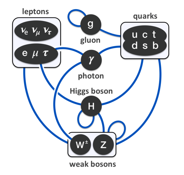
Figure 1.1: Particle interactions as described by Standard Model.

SM on the other hand, constitutes the theory of the quantum world. It successfully describes the remaining three of the four known fundamental forces of nature (electromagnetism, weak interaction and strong interaction) and additionally accommodates all the known elementary particles (see Figure 1.1). SM is the most experimentally tested theory and its predictions are confirmed with extreme accuracy. Although its phenomenal success to explain the vast majority of processes in particle physics, SM is still not capable of being the fundamental theory that describes all four fundamental forces (including gravity). Moreover, SM does not provide any insight for the nature of dark energy and dark matter, which as we already mentioned are the biggest mysteries nowadays.

It is crystal clear from the aforementioned problems that a new and more fundamental theory is needed, or a deeper understanding of the already established ideas. Such a theory should encompass both GR and SM, namely a theory of everything, but it is not necessary to be based on either of them. However, this hypothetical theory should reproduce both GR and SM in the appropriate limit. Currently, the most promising theory of unification is string theory, which replaces elementary particles with one-dimensional strings, instead of being accounted for as point-like objects. The fatal flaw of string theory is its complexity; it requires at least 10 dimensions in order to be consistent and also it is beyond experimental verification because of the extremely high energies that are needed for such a purpose.

Figure 1.2: The 5-D spacetime in Kaluza Klein theory.

Historically, the first theory that introduced extra dimensions was Kaluza-Klein theory. The primary idea came from Theodor Kaluza (1921) [12], who extended general theory of relativity by allowing the existence of another spatial dimension in addition to the four dimensional spacetime fabric of GR. Furthermore, he constrained the five-dimensional metric tensor by demanding none of its components to be dependent on the extra dimension. This condition is also known as the “cylinder condition”. His motivation for a higher dimensional spacetime was the unification of electromagnetism and gravity. The contribution of Oscar Klein (1926) [13, 14] was his quantum interpretation of Kaluza’s theory. He hypothesized that the extra dimension is curled up and tiny (see Figure 1.2) in order to explain the cylinder condition and also evaluated the scale of the extra dimension by taking into consideration the quantum nature of the electric charge.

In the last twenty years, two additional extra dimensional theories was added to the literature, ADD model (1998) [15, 16, 17] and RS models (1999) [18, 19]. Both models [15, 18] were motivated by the Hierarchy Problem and also both of them were based on the concept of braneworld, which simply indicates that Standard Model particles are confined on our 4-D spacetime (3-brane) while gravity can freely propagate in the bulk, i.e the entire $(4+n)$-dimensional spacetime, where $n$ is the number of the extra dimensions.

Particularly, the ADD model allows the existence of $n$ compact extra spatial dimensions of the same radius $R$. Thus, the total number of dimensions that gravity encounters are $(4+n)$. Subsequently, the fundamental Planck scale corresponds to the higher dimensional one, namely $M_{P(4+n)}$, while the Planck scale $M_{P}$ which we experience is an effective one. Hence, it is possible the fundamental Planck scale $M_{P(4+n)}$ to be equal to the electroweak scale $m_{EW}$ and simultaneously the effective Planck scale to maintain its huge value. As it is indicated in [15], the gravitational potential between two masses $m_{1}$ and $m_{2}$ which are separated by a distance $r\ll R$ in $(4+n)$-dimensions is given by the following expression

$$V(r)\sim\frac{m_{1}m_{2}}{M_{P(4+n)}^{n+2}}\frac{1}{r^{n+1}}$$ (1.1)

Equation (1.1) can be derived by the gravitational Gauss’s law in $(4+n)$ dimensions [20, 21]. Assuming now that $r\gg R$ we obtain

$$V(r)\sim\frac{m_{1}m_{2}}{M^{n+2}_{P(4+n)}R^{n}}\frac{1}{r}$$ (1.2)

Therefore, the effective Planck scale should fulfil the following equation

$$M_{P}^{2}\sim M_{P(4+n)}^{n+2}R^{n}$$ (1.3)

Solving the above equation with respect to $R$ and setting $M_{P(4+n)}=m_{EW}$, we obtain

$$R\sim 10^{\frac{30}{n}-19}\left(\frac{1\ TeV}{m_{EW}}\right)^{1+\frac{2}{n}}m\ \xRightarrow{m_{EW}\sim 1\ TeV}$$

$$R\sim 10^{\frac{30}{n}-19}\ m$$ (1.4)

Equation (1.4) associates the number of the extra dimensions $n$ with the size of their radius $R$. It is obvious that for $n=1$ and $R\sim 10^{11}\ m$ Newton’s gravitational law would differ from the law that we are all used to. Deviations from the conventional Newton’s law have not been measured, thus, $n\geq 2$. The upper bound for the size of the extra dimensions is $R\sim 10^{-4}\ m$ [22] and it results for $n=2$. The figures below depict schematically the two different types of topologies of the extra dimensions that was taken into consideration in [15].

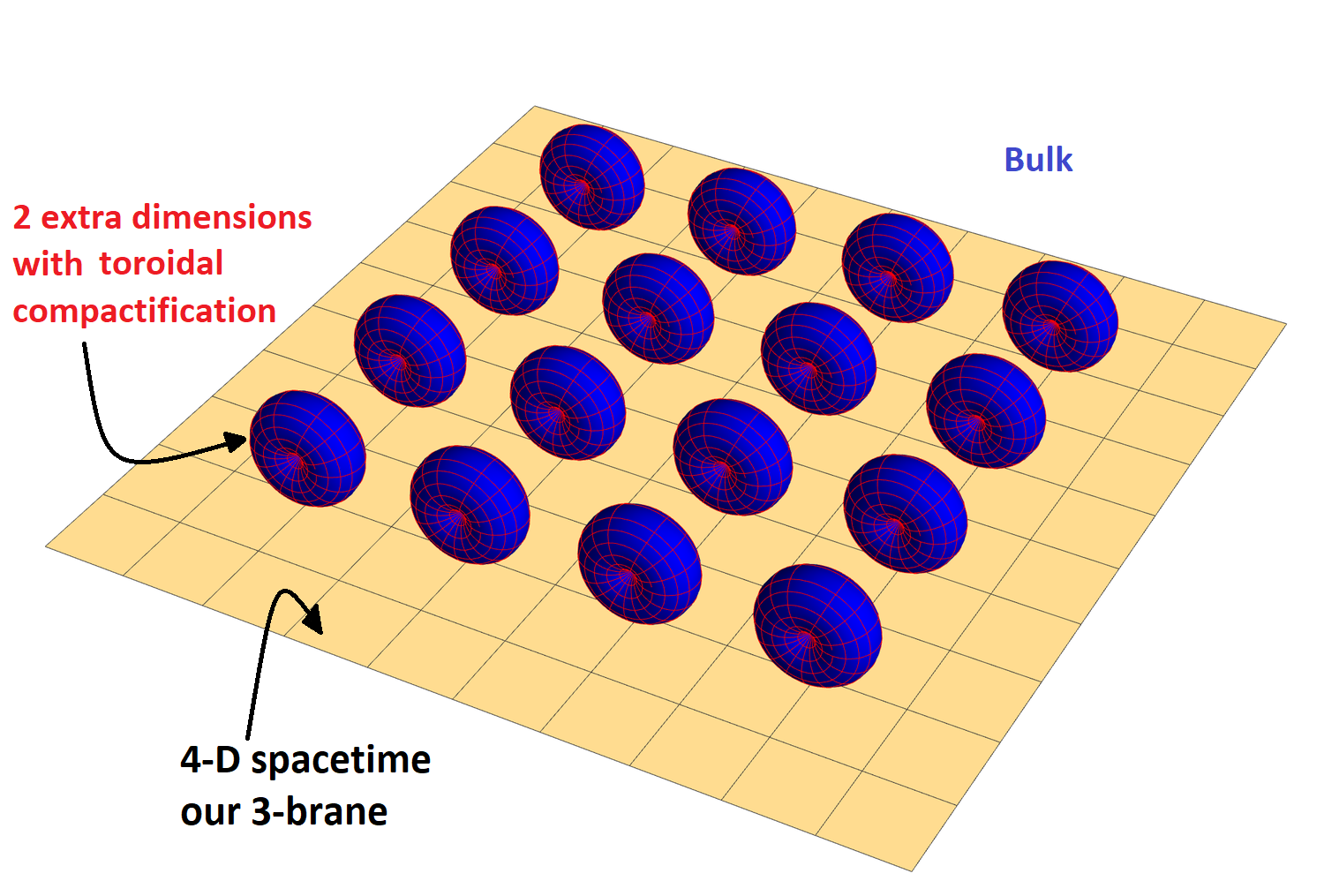
(a) toroidal compactification

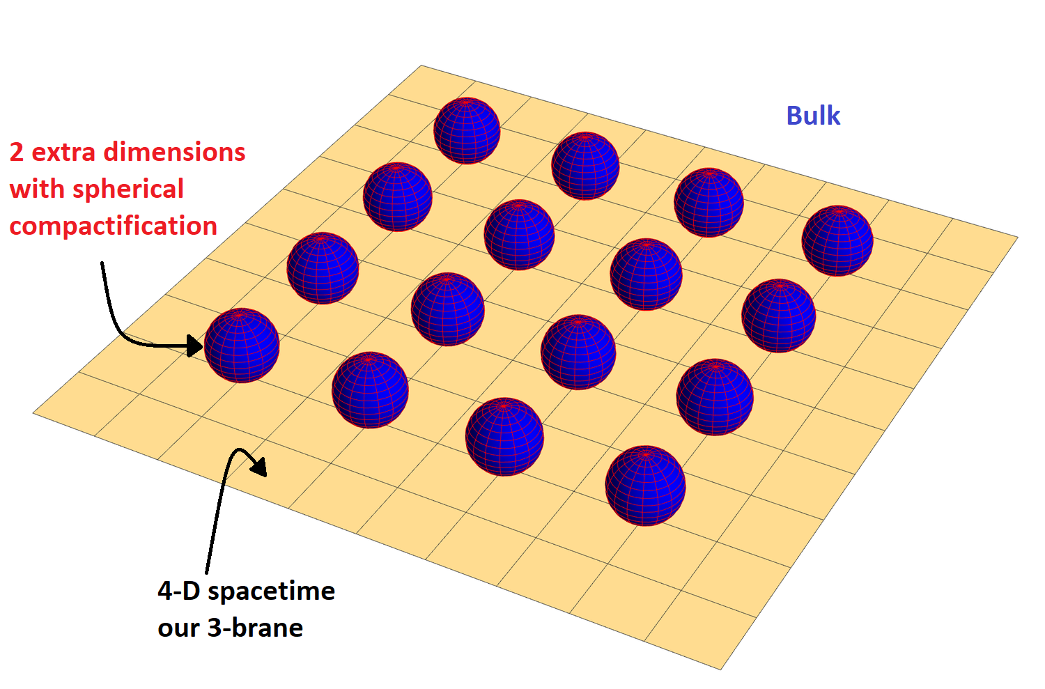
(b) spherical compactification

Figure 1.3: The 6-D spacetime in ADD model for n=2.

ADD model is elegant from a mathematical point of view, but only seemingly solves the Hierarchy Problem. In particular, ADD model simply replaces the problem of hierarchy with that of the size of the extra dimensions $R$, because now it is requisite to explain the reason why $R$ can be so much larger than the length $10^{-19}\ m$, which is associated with the fundamental Planck scale $M_{P(4+n)}=m_{EW}\sim 1\ TeV$. Although it is difficult to measure gravitational deviations of the Newton’s law in sub-millimeter distances, the fact that the fundamental gravitational scale $M_{P(4+n)}$ can be equal to $1\ TeV$ gives us the opportunity to detect (indirectly) the existence of extra dimensions in collider experiments through the formation of tiny black holes from highly energetic particles [23, 24, 25, 26, 27, 28, 29].

On the other extreme, the RS models [18, 19] -which were published only one year after the ADD model- examine the case of only but one curved extra dimension in the bulk. The special characteristic of these models is that now the 3-brane itself possesses tension, therefore it interacts gravitationally with the bulk. Particularly, the first RS model (RS1) assumes the existence of two 3-branes in the bulk and achieves to generate the electroweak scale from the Planck scale through an exponential hierarchy, which arises purely from the geometry of the 5-D spacetime. RS2 model assumes the existence of only one 3-brane embedded in an infinitely long extra dimension but nevertheless manages to reproduce 4-dimensional gravity on the brane. Both RS models will be discussed in Chapter 2, thus, any further detail will be postponed for later.

1.1 Motivation and Thesis outline

In the context of GR, all the information that is needed to describe a black hole comes only from three classical parameters: mass $(M)$, electric charge $(Q)$ and angular momentum $(J)$. It is impossible to distinguish two black holes if they are characterized by the same aforementioned parameters and these parameters have the same value. This is an incredible characteristic of the 4-D black holes and it is rarely encountered in other objects in nature. Given these parameters, there are only four different black hole solutions [11, 30, 31, 32] that can be derived by the gravitational field equations of GR; this particular statement is also known as the no-hair theorem [33, 34, 35]. On the other hand, braneworld black holes are not so easily manageable and most importantly there is not a corresponding no-hair theorem for higher dimensional spacetimes. Therefore, the “families” of higher dimensional black holes solutions are not yet known. This thesis is entirely focused on braneworld black holes and more specifically on the existence of localized black hole solutions in an RS2-type braneworld model.

The outline of the thesis is as follows. Chapter 2 -as it was mentioned previously- constitutes a detailed analysis of the RS models. The existence of black string solutions in the context of RS models and the difficulties in finding a localized 5-D black hole solution on our 3-brane are reviewed in Chapter 3. In the same Chapter, the theoretical framework of the thesis, namely the geometrical background that the thesis is based on, and the scalar field theory (two non-minimally-coupled and interacting scalar fields with a general coupling to the Ricci scalar) are also presented. This scalar field theory constitutes a more general theory compared to the scalar field theory that is presented in [36]. This extra degree of freedom -that the additional scalar field offers- may lead to a solution to the problem of localizing a 5-dimensional black hole on a 3-brane. Finally, in Chapter 3, the field equations of this particular ansatz are derived. Subsequently, the various cases which are studied in this particular scenario are presented in a series of paragraphs of increasing complexity in Chapter 4. Finally, our results and our conclusions are discussed in Chapter 5.

Chapter 2 Randall-Sundrum Brane-World Models

In their first model [18] (RS1), Lisa Randall and Raman Sundrum introduced a compact extra dimension, which is finite and bounded by two 3-branes. This specific type of spacetime enriched with some additional properties, which are going to be discussed in the following section, manages to address the hierarchy problem. Amazingly, they proved that the 4-D gravity can also be recovered on the brane even if the extra dimension has infinite size, this constitutes the RS2 model [19]. Let us now proceed to the analysis of these models.

2.1 RS1 Model

The RS model postulates the existence of one extra dimension which is compactified on a circle $S^{1}$ (one-dimensional sphere) and also possesses a $\mathbb{Z}_{2}$ symmetry, which simply means that the points $(x^{\mu},y)$ and $(x^{\mu},-y)$ are identified. Hence, the extra dimension is an $S^{1}/\mathbb{Z}_{2}$ orbifold. As it is illustrated in the figure below, this type of compactification contains two fixed points, at $y=0$ and $y=\pi r_{c}\equiv L$. The range of $y$ is from $-L$ to $L$, but the metric is completely specified by the values in the range $0\leq y\leq L$. These fixed points of the extra dimension ($y=0$ and $y=L$) host the two 3-branes, which essentially are two separated 4-D worlds.

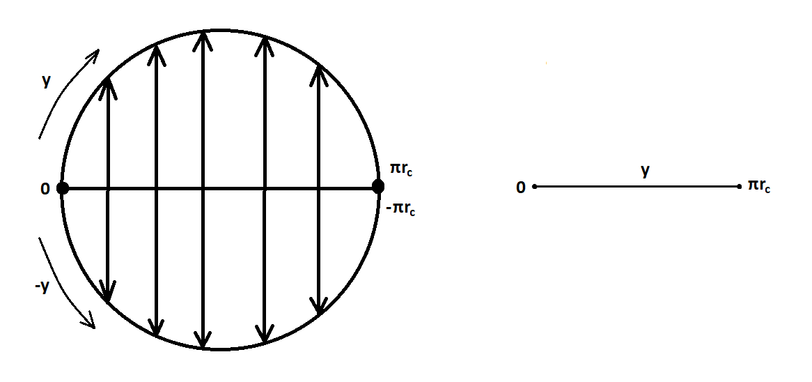
Figure 2.1: $S^{1}/\mathbb{Z}_{2}$ orbifold

The action of the model is as follows:

$$S=S_{grav}+S_{1}+S_{2}$$ (2.1)

$$S_{grav}=\int d^{4}x\int_{-L}^{L}dy\ \sqrt{-g^{(5)}}\left(\frac{R}{2\kappa_{(5)}}-\Lambda_{5}\right)$$ (2.2)

$$S_{1}=\int d^{4}x\sqrt{-g_{1}}\ (\mathcal{L}_{1}-\sigma_{1})$$ (2.3)

$$S_{2}=\int d^{4}x\sqrt{-g_{2}}\ (\mathcal{L}_{2}-\sigma_{2})$$ (2.4)

where

$$g^{(5)}=\det\left[g_{MN}(x^{\lambda},y)\right]$$ (2.5)

$$g_{1}=\det\left[g^{1}_{\mu\nu}(x^{\lambda})\right]$$ (2.6)

$$g_{2}=\det\left[g^{2}_{\mu\nu}(x^{\lambda})\right]$$ (2.7)

The determinants $g_{1}$ and $g_{2}$ are derived by the metrics $g^{1}_{\mu\nu}$ and $g_{\mu\nu}^{2}$ of the two 3-branes which are located at $y=0$ and $y=L$ respectively. $R$ is the 5-D Ricci scalar, $\Lambda_{5}$ is the higher dimensional cosmological constant and $\kappa_{(5)}=8\pi G_{(5)}=M_{P(5)}^{-3}$ where $M_{P(5)}$ is the fundamental Planck scale of the 5-D spacetime. The quantities $\sigma_{1}$ and $\sigma_{2}$ represent the energy densities of the 3-branes, while $\mathcal{L}_{1}$ and $\mathcal{L}_{2}$ are the Lagrangians on each 3-brane.

The variation of Eq.(2.1) with respect to the components of the 5-D metric tensor $g_{MN}$ provides us with the field equations (see Appendix F for more details about the variation of a general action). The field equations, which are depicted below, were deduced under the assumption that $\mathcal{L}_{1}=\mathcal{L}_{2}=0$. This particular assumption was made in order to determine the geometrical background of the model. The field equations have the following form:

$$\sqrt{-g^{(5)}}\ G_{MN}=-\kappa_{(5)}\left[\sqrt{-g^{(5)}}\ g_{MN}\ \Lambda_{5}\right. +\sqrt{-g_{1}}\ \sigma_{1}\ g^{1}_{\mu\nu}\ \delta^{\mu}_{M}\ \delta^{\nu}_{N}\ \delta(y)$$

$$\left.+\sqrt{-g_{2}}\ \sigma_{2}\ g^{2}_{\mu\nu}\ \delta^{\mu}_{M}\ \delta^{\nu}_{N}\ \delta(y-L)\right]$$ (2.8)

In order to continue the analysis of the model it is necessary to introduce an appropriate metric for such a setup. A property that we need to impose on the 5-D metric is to respect the Poincaré symmetry on the two 3-branes. This property comes naturally from the fact that the 4-D induced metrics on the 3-branes should describe the real world and therefore they should respect the same symmetries as the physical world. The general form of a five-dimensional line-element that includes an extra dimension with $S^{1}/\mathbb{Z}_{2}$ compactification and also respects Poincaré symmetry has the following form

$$ds^{2}=e^{2A(y)}\eta_{\mu\nu}dx^{\mu}dx^{\nu}+dy^{2}$$ (2.9)

The function $A(y)$ is called warp factor and it will be evaluated subsequently by the gravitational field equations of this theory. It is obvious that the metric tensor that results from this particular line-element is of the form

$$(g_{MN})=\left(\begin{array}[]{ccccc}-e^{2A(y)}&0&0&0&0\\ 0&e^{2A(y)}&0&0&0\\ 0&0&e^{2A(y)}&0&0\\ 0&0&0&e^{2A(y)}&0\\ 0&0&0&0&1\end{array}\right)$$ (2.15)

$$g_{MN}=\underbrace{e^{2A(y)}\eta_{\mu\nu}}_{g_{\mu\nu}}\delta^{\mu}_{M}\delta^{\nu}_{N}+\delta^{4}_{M}\delta^{4}_{N}=g_{\mu\nu}\delta^{\mu}_{M}\delta^{\nu}_{N}+\delta^{4}_{M}\delta^{4}_{N}$$ (2.16)

$$(g^{MN})=\left(\begin{array}[]{ccccc}-e^{-2A(y)}&0&0&0&0\\ 0&e^{-2A(y)}&0&0&0\\ 0&0&e^{-2A(y)}&0&0\\ 0&0&0&e^{-2A(y)}&0\\ 0&0&0&0&1\\ \end{array}\right)$$ (2.22)

$$g^{MN}=\underbrace{e^{-2A(y)}\eta^{\mu\nu}}_{g^{\mu\nu}}\delta_{\mu}^{M}\delta_{\nu}^{N}+\delta_{4}^{M}\delta_{4}^{N}=g^{\mu\nu}\delta_{\mu}^{M}\delta_{\nu}^{N}+\delta_{4}^{M}\delta_{4}^{N}$$ (2.23)

Consequently, the induced metric tensors on the 3-branes at the points $y=0$ and $y=L$ are given by

$$g^{1}_{\mu\nu}=e^{2A(0)}\eta_{\mu\nu}$$ (2.24)

$$g^{2}_{\mu\nu}=e^{2A(L)}\eta_{\mu\nu}$$ (2.25)

The non-zero and two-times covariant components of the Einstein tensor $G_{MN}$ of the aforementioned ansatz are depicted below:

$$\left\{\begin{array}[]{c}G_{00}=G_{tt}=-3e^{2A(y)}\left[2A^{\prime 2}(y)+A^{\prime\prime}(y)\right]\\ \\ G_{11}=G_{22}=G_{33}=3e^{2A(y)}\left[2A^{\prime 2}(y)+A^{\prime\prime}(y)\right]\\ \\ G_{44}=G_{yy}=6A^{\prime 2}(y)\end{array}\right\}\Rightarrow\left\{\begin{array}[]{c}G_{\mu\nu}=3\left[2A^{\prime 2}(y)+A^{\prime\prime}(y)\right]g_{\mu\nu}\\ \\ G_{44}=6A^{\prime 2}(y)\end{array}\right\}$$ (2.26)

Combining equations (2.1), (2.16) and (2.26) for $M=N=4$ we get:

$$6A^{\prime 2}(y)=-\kappa_{(5)}\Lambda_{5}\Rightarrow A^{\prime 2}(y)=-\frac{\kappa_{(5)}\Lambda_{5}}{6}$$ (2.27)

while for $M=\mu$ and $N=\nu$ we obtain:

$$6A^{\prime 2}(y)+3A^{\prime\prime}(y)=-\kappa_{(5)}\Lambda_{5}-\kappa_{(5)}\ \sigma_{1}\ \delta(y)-\kappa_{(5)}\ \sigma_{2}\ \delta(y-L)\xRightarrow{\eqref{rs17}}$$

$$3A^{\prime\prime}(y)=-\kappa_{(5)}\left[\sigma_{1}\ \delta(y)+\sigma_{2}\ \delta(y-L)\right]\Rightarrow$$

$$A^{\prime\prime}(y)=-\frac{\kappa_{(5)}}{3}\left[\sigma_{1}\ \delta(y)+\sigma_{2}\ \delta(y-L)\right]$$ (2.28)

The five-dimensional cosmological constant $\Lambda_{5}$ must be negative in order to have a real solution for the function $A(y)$. A negative 5-D cosmological constant affects decisively the geometry of the spacetime between the two 3-branes. Particularly, the bulk spacetime of this scenario leads to an anti-de Sitter spacetime between the two branes, which is also denoted as $AdS_{5}$. Subsequently, we define the following constant

$$\boxed{k^{2}\equiv-\frac{\kappa_{(5)}\Lambda_{5}}{6}}$$ (2.29)

The specific function of $A(y)$ can be easily deduced from Eq.(2.27). Combining equations (2.27) and (2.29), we get

$$A^{\prime 2}(y)=k^{2}\Rightarrow A^{\prime}(y)=\pm k\Rightarrow A(y)=\pm ky\Rightarrow\boxed{A(y)=-k|y|}$$ (2.30)

The reason that we kept the minus sign in Eq.(2.30) will be understood later. In addition, it is necessary to preserve the orbifold symmetry $S_{1}/\mathbb{Z}_{2}$ for the extra dimension $y$. Hence, we are obliged to express the function $A(y)$ in terms of $|y|$. Substituting Eq.(2.30) into Eq.(2.9) we obtain the geometrical background of the RS model:

$$\boxed{ds^{2}=e^{-2k|y|}\eta_{\mu\nu}dx^{\mu}dx^{\nu}+dy^{2}}$$ (2.31)

We can relate the constants $\sigma_{1}$ and $\sigma_{2}$ with $k$ by evaluating the second derivative of $A(y)$ as given by Eq.(2.30) and then equate the result with Eq.(2.28).

$$A^{\prime}(y)=-k(|y|)^{\prime}=-k\ sgn(y)=-k\left[H(y)-H(-y)\right]$$ (2.32)

where

$$H(y)=\left\{\begin{array}[]{cr}0,&-L\leq y<0\\ \\ 1,&0\leq y\leq L\end{array}\right\}\hskip 5.0pt,\hskip 15.00002ptH(-y)=\left\{\begin{array}[]{cr}1,&-L\leq y<0\\ \\ 0,&0\leq y\leq L\end{array}\right\}$$ (2.33)

$$A^{\prime\prime}(y)=-k\left[H^{\prime}(y)-H^{\prime}(-y)\right]=-2k\left[\delta(y)-\delta(y-L)\right]$$ (2.34)

where

$$\left\{\begin{gathered}H^{\prime}(y)=\delta(y)-\delta(y-L)\\ \\ H^{\prime}(-y)=\delta[-(y-L)]-\delta(-y)=-\delta(y)+\delta(y-L)\end{gathered}\right\}$$ (2.35)

$$\eqref{rs18}\xRightarrow{\eqref{rs25}}-\frac{\kappa_{(5)}}{3}\left[\sigma_{1}\ \delta(y)+\sigma_{2}\ \delta(y-L)\right]=-2k\left[\delta(y)-\delta(y-L)\right]\Rightarrow$$

$$\boxed{\sigma_{1}=-\sigma_{2}=\frac{6k}{\kappa_{(5)}}}$$ (2.36)

Let us now focus on the 3-brane at $y=L$ and include the Higgs field in the 4-dimensional action. We are going to evaluate the Vacuum Expectation Value (VEV) of the Higgs field on the brane which determines the physical masses in the Standard Model. The action will have the form:

$$S_{H}=\int d^{4}x\int_{-L}^{L}dy\sqrt{-g^{(5)}}\left[g^{MN}D_{M}H^{\dagger}D_{N}H-\lambda(H^{\dagger}H-v_{0}^{2})^{2}\right]\delta(y-L)\Rightarrow$$

$$S_{H}=\int d^{4}x\sqrt{-g_{2}}\left[g_{2}^{\mu\nu}D_{\mu}H^{\dagger}D_{\nu}H-\lambda(|H|^{2}-v_{0}^{2})^{2}\right]\xRightarrow[\sqrt{-g_{2}}=e^{4A(L)}=e^{-4kL}]{g_{2}^{\mu\nu}=e^{-2A(L)}\eta^{\mu\nu}=e^{2kL}\eta^{\mu\nu}}$$

$$S_{H}=\int d^{4}x\ e^{-4kL}\left[e^{2kL}\eta^{\mu\nu}D_{\mu}H^{\dagger}D_{\nu}H-\lambda(|H|^{2}-v_{0}^{2})^{2}\right]\Rightarrow$$

$$S_{H}=\int d^{4}x\left[\eta^{\mu\nu}D_{\mu}\tilde{H}^{\dagger}D_{\nu}\tilde{H}-\lambda(|\tilde{H}|^{2}-v^{2})^{2}\right]$$ (2.37)

In order to obtain a canonically normalized action we defined

$$\tilde{H}\equiv e^{-kL}H$$ (2.38)

$$v\equiv e^{-kL}v_{0}$$ (2.39)

The action of Eq.(2.37) depicts the ordinary action of the Higgs field. The corresponding VEV of the renormalized Higgs scalar $\tilde{H}$ is $v$ and is given by Eq.(2.39), while the Higgs scalar $H$ is the bare Higgs with VEV $v_{0}$. As we mentioned earlier, the VEV of the Higgs field determines all the mass parameters in the context of SM, thus we can safely conclude that

$$\boxed{m=e^{-kL}m_{0}}$$ (2.40)

where $m$ constitutes the physical mass as it is measured on the 3-brane at $y=L$. Eq.(2.40) is a simple and “powerful” result. It can be considered as a necessary condition for the solution of the hierarchy problem, because it does not demand a huge discrepancy between parameters $k$ and $L$ in order to achieve that. It is easy to verify the previous statement by setting $m_{0}$ equal to the Planck mass $M_{P}\sim 10^{18}\ GeV$ and $m$ equal to the electroweak scale $m_{EW}\sim 1\ TeV$. Then:

$$10^{3}\ GeV=e^{-kL}\ 10^{18}\ GeV\Rightarrow e^{-kL}=10^{-15}\Rightarrow kL=15\ln(10)\Rightarrow$$

$$\boxed{kL\approx 35}$$ (2.41)

In order to confidently state that the type of exponential suppression of Eq.(2.40) successfully addresses the hierarchy problem, it is also necessary to examine the dependence of the effective scale (4-D scale) of gravity on the size of the extra dimension $y$. For this purpose, we need to perturb the four-dimensional part of the five-dimensional line-element of Eq.(2.31) and then extract the 4-D gravitational action from the original 5-D action which is shown at Eq.(2.2). The form of the perturbative line-element is given by the following relation:

$$ds^{2} =e^{-2k|y|}[\eta_{\mu\nu}+h_{\mu\nu}(x)]dx^{\mu}dx^{\nu}+dy^{2}$$

$$=e^{-2k|y|}g^{per}_{\mu\nu}dx^{\mu}dx^{\nu}+dy^{2}$$ (2.42)

where $|h_{\mu\nu}|\ll 1$. Using the metric that follows from Eq.(2.1) into Eq.(2.2) and focusing on the term which includes the Ricci scalar, we obtain

$$S_{eff}=\int d^{4}x\int_{-L}^{L}dy\ \frac{e^{-2k|y|}}{2\kappa_{(5)}}\sqrt{-g_{per}}\ R^{4D}(g^{per}_{\mu\nu})$$ (2.43)

The $S_{eff}$ should be also equal to

$$S_{eff}=\int d^{4}x\sqrt{-g_{per}}\ \frac{R^{4D}}{2\kappa}$$ (2.44)

where $\kappa=8\pi G=M_{P}^{-2}$. Consequently, by equating the last two relations we obtain the following expression for the effective scale of gravity.

$$\frac{1}{\kappa}=\frac{1}{\kappa_{(5)}}\int_{-L}^{L}dy\ e^{-2k|y|}\Rightarrow M_{P}^{2}=M_{P(5)}^{3}\left(\int_{-L}^{0}dy\ e^{2ky}+\int_{0}^{L}dy\ e^{-2ky}\right)\Rightarrow$$

$$M_{P}^{2}=M_{P(5)}^{3}\left(\frac{1}{2k}-\frac{e^{-2kL}}{2k}-\frac{e^{-2kL}}{2k}+\frac{1}{2k}\right)\Rightarrow M_{P}^{2}=\frac{M_{P(5)}^{3}}{k}\left(1-e^{-2kL}\right)\Rightarrow$$

$$\boxed{M_{P}^{2}=\frac{M_{P(5)}^{3}}{k}\left(1-e^{-2kL}\right)}$$ (2.45)

Substituting now the value of the product $kL$ given by Eq.(2.41) into Eq.(2.45) we get

$$M_{P}^{2}=\frac{M_{P(5)}^{3}}{k}(1-e^{-70})\simeq\frac{M_{P(5)}^{3}}{k}$$ (2.46)

It is clear from Eq.(2.45) and Eq.(2.46) that gravity is essentially independent of the size of the extra dimension. Surprisingly, even if we infinitely extend the length $L$ of the extra dimension in Eq.(2.45), the four-dimensional Planck scale $M_{P}$ remains finite. This particular observation was the central point of the RS2 model which is going to be analyzed in the section that follows.

Conclusively, it was shown that in the context of the RS model the hierarchy problem has an extremely simple and clear solution. Simultaneously, the RS model does not introduce new huge hierarchies (in contrast with the ADD model) between its fundamental parameters ($k$, $\kappa_{(5)}$ or $M_{P(5)}$, $v_{0}$, $L$ or $r_{c}$). The only constraint that is required by the model is that $kL\approx 35$. Of course, a stabilizing mechanism (Goldberger-Wise mechanism [37, 38]) must be included in the model for this purpose but this is beyond the context of the present analysis.

2.2 RS2 Model

In their second paper, Lisa Randall and Raman Sundrum proved that is in fact possible to extend the length $L$ of the extra dimension to an infinite value and nevertheless get an effectively four-dimensional gravity. The verification of the previous statement is derived from the fact that the 5-D graviton is localized near the 3-brane at $y=0$. The setup of the RS2 model is similar to the RS1 model with the difference that the 3-brane at $y=L$ is practically removed from the original picture, by taking $L$ to infinity. Thus, the action of the RS2 model is

$$S=S_{grav}+S_{1}$$ (2.47)

$$S_{grav}=\int d^{4}x\int dy\ \sqrt{-g^{(5)}}\left(\frac{R}{2\kappa_{(5)}}-\Lambda_{5}\right)$$ (2.48)

$$S_{1}=\int d^{4}x\sqrt{-g_{1}}\left(\mathcal{L}_{1}-\sigma_{1}\right)$$ (2.49)

The line-element of the RS2 model is given by Eq.(2.16) as well. Let us now proceed to the derivation of the graviton modes.

Gravitons correspond to small fluctuations in the spacetime “fabric”. Therefore, in the context of RS2 model we have

$$ds^{2}=e^{-2k|y|}\left[\eta_{\mu\nu}+h_{\mu\nu}(x,y)\right]dx^{\mu}dx^{\nu}+dy^{2}$$ (2.50)

In the last equation it was chosen $h_{M4}=0$. It is always possible to find a set of coordinates with this particular property in the region of the 3-brane. We now seek a new variable $z$ for the description of the extra dimension in order to construct a metric tensor which will be more convenient for future calculations. For this purpose, we demand from the new variable $z$ to satisfy the following relation:

$$dy^{2}\equiv e^{-2k|y|}dz^{2}$$ (2.51)

Performing the integration of the previous equation we find

$$k|z|=e^{k|y|}-1$$ (2.52)

where we chose the integration constant appropriately in order to get $z=0$ when $y=0$. Eq.(2.52) leads to

$$e^{-2k|y|}=\frac{1}{(k|z|+1)^{2}}$$ (2.53)

Combining equations (2.50) and (2.53) we obtain

$$ds^{2}=\frac{1}{(k|z|+1)^{2}}\left\{\left[\eta_{\mu\nu}+h_{\mu\nu}(x,z)\right]dx^{\mu}dx^{\nu}+dz^{2}\right\}\xRightarrow{h_{4M}=0}$$

$$ds^{2}=e^{2A(z)}\left[\eta_{MN}+h_{MN}(x,z)\right]dx^{M}dx^{N}\Rightarrow$$

$$\boxed{ds^{2}=e^{2A(z)}\bar{g}_{MN}(x,z)dx^{M}dx^{N}}$$ (2.54)

where

$$\boxed{e^{2A(z)}\equiv\frac{1}{(k|z|+1)^{2}}}$$ (2.55)

$$\boxed{\bar{g}_{MN}(x,z)\equiv\eta_{MN}+h_{MN}(x,z)}$$ (2.56)

From Eq.(2.55) we get

$$A(z)=-\ln(k|z|+1)$$ (2.57)

$$A^{\prime}(z)=-\frac{k\ sgn(z)}{k|z|+1}=-\frac{k[H(z)-H(-z)]}{k|z|+1}$$ (2.58)

$$A^{\prime\prime}(z)=-\frac{2k\delta(z)}{k|z|+1}+\frac{k^{2}}{(k|z|+1)^{2}}$$ (2.59)

Under the above transformation of the extra dimension (from $y$ to $z$), Eq.(2.48) is also going to be transformed into

$$S_{grav}=\int d^{4}x\int_{-L_{z}}^{L_{z}}dz\sqrt{-g^{(5)}}\left(\frac{R}{2\kappa_{(5)}}-\Lambda_{5}\right)$$ (2.60)

where $L_{z}=(e^{kL}-1)/k$. The field equations which are yielded by the variation of Eq.(2.47) with respect to the components of the 5-D metric are depicted below ($\mathcal{L}_{1}$ in Eq.(2.49) is set to be 0).

$$\sqrt{-g^{(5)}}\ G_{MN}=-\kappa_{(5)}\left[\sqrt{-g^{(5)}}\ g_{MN}\ \Lambda_{5}+\sqrt{-g_{1}}\ g^{1}_{\mu\nu}\ \delta^{\mu}_{M}\ \delta^{\nu}_{N}\ \delta(z)\ \sigma_{1}\right]$$ (2.61)

where

$$g^{1}_{\mu\nu}\ \delta(z)=e^{2A(z)}(\eta_{\mu\nu}+h_{\mu\nu})\ \delta(z)$$ (2.62)

$$g_{1}\ \delta(z)=g^{(5)}\ e^{-2A(z)}\ \delta(z)$$ (2.63)

Hence, the combination of equations (2.61)-(2.63) results to

$$G_{MN}=-\kappa_{(5)}\left[g_{MN}\ \Lambda_{5}+e^{A(z)}(\eta_{\mu\nu}+h_{\mu\nu})\delta^{\mu}_{M}\ \delta^{\nu}_{N}\ \delta(z)\ \sigma_{1}\right]$$ (2.64)

The calculation of the Einstein tensor components $G_{MN}$ using “brute force” is a difficult task in this model. Hence, we are going to use a conformal transformation in order to obtain the components of the Einstein tensor more easily. Particularly, we mention (without proof) that if $\tilde{g}_{MN}$ is the conformally transformed metric of the metric $g_{MN}$ and the two metrics are connected through the relation

$$\tilde{g}_{MN}=\Omega^{2}(x,z)\ g_{MN}$$ (2.65)

then the corresponding components of the Einstein tensor are connected as follows:

$$\tilde{G}_{MN}=G_{MN}+\frac{D-2}{2\Omega^{2}}\left[4\Omega_{,M}\Omega_{,N}+(D-5)\Omega_{,K}\Omega^{,K}\ g_{MN}\right]-\frac{D-2}{\Omega}\left(\Omega_{;MN}-g_{MN}\square\Omega\right)$$ (2.66)

where $D$ indicates the total number of spacetime’s dimensions. The adjustment of equations (2.65) and (2.66) in our case is straightforward. We simply execute the following substitutions: {$\tilde{g}_{MN}\rightarrow g_{MN}$, $\Omega(x,z)\rightarrow e^{A(z)}$, $g_{MN}\rightarrow\bar{g}_{MN}$ and $D=5$}. Hence, we obtain the expression:

$$G_{MN}=\bar{G}_{MN}+3\left[\partial_{M}A\ \partial_{N}A-\nabla_{M}\nabla_{N}A+\bar{g}_{MN}(\square A+\partial_{L}A\ \partial^{L}A)\right]\Rightarrow$$

$$G_{MN}=\bar{G}_{MN}+3[\partial_{M}A\ \partial_{N}A -\partial_{M}\partial_{N}A+\bar{\Gamma}^{L}{}_{MN}\partial_{L}A$$

$$+\bar{g}_{MN}(\partial_{L}\partial^{L}A+\bar{\Gamma}^{L}{}_{LK}\partial^{K}A+\partial_{L}A\ \partial^{L}A)]$$ (2.67)

For all the subsequent calculations in this section, the terms which contain fluctuations $(h_{MN})$ of order higher than the first will be neglected. Additionally, it is possible and extremely convenient to perform appropriate coordinate transformations in which the fluctuations satisfy the following properties:

$$\left\{\begin{array}[]{c}h_{4M}=0\\ \\ h=h^{\mu}{}_{\mu}=0\\ \\ \partial_{\mu}h^{\mu}{}_{\nu}=0\end{array}\right\}$$ (2.68)

In this gauge and with the use of equations (C.3) and (C.8) it is quite trivial to show that the Christoffel symbols $\bar{\Gamma}^{L}{}_{MN}$ and the components of Einstein tensor $\bar{G}_{MN}$ are expressed through the following equations:

$$\bar{\Gamma}^{L}{}_{MN}=\frac{1}{2}\left(\partial_{N}h^{L}{}_{M}+\partial_{M}h^{L}{}_{N}-\partial^{L}h_{MN}\right)$$ (2.69)

$$\bar{G}_{MN}=-\frac{1}{2}\partial_{L}\partial^{L}h_{MN}$$ (2.70)

Using equations (2.2)-(2.70) we are led to

$$\left\{\begin{array}[]{c}G_{44}=6A^{\prime 2}\\ \\ G_{4\mu}=0\\ \\ G_{\mu\nu}=-\frac{1}{2}\partial_{L}\partial^{L}h_{\mu\nu}-\frac{3}{2}\ \partial_{4}h_{\mu\nu}\ A^{\prime}+3(\eta_{\mu\nu}+h_{\mu\nu})(A^{\prime\prime}+A^{\prime 2})\end{array}\right\}$$ (2.71)

The combination of equations (2.64) and (2.71) for $M=N=4$ results to Eq.(2.57), namely

$$6A^{\prime 2}=-\kappa_{(5)}\Lambda_{5}\ g_{44}=-\kappa_{(5)}\Lambda_{5}\ e^{2A(z)}(\underbrace{\eta_{44}}_{1}+\underbrace{h_{44}}_{0})\xRightarrow{\eqref{rs19}}A^{\prime 2}(z)=k^{2}e^{2A(z)}\Rightarrow$$

$$A(z)=-\ln(k|z|+1)$$

where we fixed again the integration constant appropriately (the reason has already been discussed in the sentence before equation (2.53)). Correspondingly, for $M=\mu$ and $N=\nu$ we have:

$$-\frac{1}{2}\partial_{L}\partial^{L}h_{\mu\nu}-\frac{3}{2}\ \partial_{4}h_{\mu\nu}\ A^{\prime}+3(\eta_{\mu\nu}+h_{\mu\nu})(A^{\prime\prime}+A^{\prime 2})=-\kappa_{(5)}(\eta_{\mu\nu}+h_{\mu\nu})[e^{2A}\Lambda_{5}+e^{A}\delta(z)\ \sigma_{1}]$$ (2.72)

It is not hard to combine equations (2.29), (2.36), (2.55), (2.58) and (2.59) in order to prove the following expressions (these are going to simplify Eq.(2.72) afterwards):

$$-\kappa_{(5)}\Lambda_{5}\ e^{2A(z)}=-\frac{\kappa_{(5)}\Lambda_{5}}{6}\ 6\ e^{2A(z)}=6\ k^{2}\ e^{2A(z)}=6A^{\prime 2}(z)$$ (2.73)

$$-\kappa_{(5)}\ \sigma_{1}\ e^{A(z)}\ \delta(z)=-6\ k\ e^{A(z)}\ \delta(z)=3[A^{\prime\prime}(z)-A^{\prime 2}(z)]$$ (2.74)

Consequently, from equations (2.72)-(2.74) we get

$$\boxed{\partial_{L}\partial^{L}h_{\mu\nu}+3\ \partial_{4}h_{\mu\nu}\ A^{\prime}=0}$$ (2.75)

We now rescale the fluctuations $h_{\mu\nu}$ as follows.

$$h_{\mu\nu}\rightarrow e^{\lambda A(z)}h_{\mu\nu}$$ (2.76)

Then, Eq.(2.75) takes the form:

$$h_{\mu\nu}\left[(3\lambda+\lambda^{2})A^{\prime 2}+\lambda\ A^{\prime\prime}\right]+(2\lambda+3)A^{\prime}\ \partial_{4}h_{\mu\nu}+\partial_{L}\partial^{L}h_{\mu\nu}=0$$ (2.77)

It is now obvious that we can nullify the term which contains the quantity $\partial_{4}h_{\mu\nu}$ by choosing $\lambda=-3/2$. Furthermore, we perform a Kaluza-Klein decomposition on the fluctuations $h_{\mu\nu}(x,z)$:

$$h_{\mu\nu}(x,z)=\sum_{n=0}^{\infty}h_{\mu\nu}^{n}(x)\psi_{n}(z)$$ (2.78)

where

$$\left\{\begin{array}[]{c}h^{n}_{\mu\nu}(x)=e^{ip_{n}x}=e^{ip^{n}_{\lambda}x^{\lambda}}\\ \\ \partial_{\sigma}\partial^{\sigma}h_{\mu\nu}^{n}(x)=m_{n}^{2}\ h_{\mu\nu}^{n}(x)\end{array}\right\}$$ (2.79)

Substituting equations (2.78) and (2.79) into Eq.(2.77) and setting $\lambda=-3/2$, we obtain

$$\partial_{L}\partial^{L}\left[\sum_{n=0}^{\infty}h^{n}_{\mu\nu}(x)\psi_{n}(z)\right]-\left(\frac{3}{2}A^{\prime\prime}+\frac{9}{4}A^{\prime 2}\right)\sum_{n=0}^{\infty}h^{n}_{\mu\nu}(x)\psi_{n}(z)=0\Rightarrow$$

$$\partial_{4}\partial^{4}\left[\sum_{n=0}^{\infty}h^{n}_{\mu\nu}(x)\psi_{n}(z)\right]+\partial_{\sigma}\partial^{\sigma}\left[\sum_{n=0}^{\infty}h^{n}_{\mu\nu}(x)\psi_{n}(z)\right]-\left(\frac{3}{2}A^{\prime\prime}+\frac{9}{4}A^{\prime 2}\right)\sum_{n=0}^{\infty}h^{n}_{\mu\nu}(x)\psi_{n}(z)=0\Rightarrow$$

$$\sum_{n=0}^{\infty}\left\{h^{n}_{\mu\nu}(x)\left[\psi_{n}^{\prime\prime}(z)+m_{n}^{2}\ \psi_{n}(z)-\left(\frac{3}{2}A^{\prime\prime}+\frac{9}{4}A^{\prime 2}\right)\psi_{n}(z)\right]\right\}=0\Rightarrow$$

$$\boxed{-\psi_{n}^{\prime\prime}(z)+V(z)\ \psi_{n}(z)=m_{n}^{2}\ \psi_{n}(z)}$$ (2.80)

where

$$\boxed{V(z)=\frac{3}{2}A^{\prime\prime}+\frac{9}{4}A^{\prime 2}=-\frac{3k\delta(z)}{k|z|+1}+\frac{15k^{2}}{4(k|z|+1)^{2}}=\frac{15k^{2}}{4(k|z|+1)^{2}}-3k\delta(z)}$$ (2.81)

The boundary condition at $z=0$ can be found as follows:

$$\eqref{rs70}\Rightarrow\int_{0^{-}}^{0^{+}}dz\left[-\psi_{n}^{\prime\prime}(z)+V(z)\psi(z)\right]=\int_{0^{-}}^{0^{+}}dz\ m_{n}^{2}\ \psi_{n}(z)\Rightarrow$$

$$-\psi_{n}^{\prime}(0^{+})+\psi_{n}^{\prime}(0^{-})-3k\psi_{n}(0)=0\xRightarrow[\psi^{\prime}_{n}(z)=-\psi^{\prime}_{n}(-z)]{\psi_{n}(z)=\psi_{n}(-z)}$$

$$\boxed{\psi^{\prime}_{n}(0^{+})=-\frac{3}{2}\ k\ \psi_{n}(0)}$$ (2.82)

Although we have focused on the RS2 model, we may develop a unified analysis for the study of gravitons in both RS models. Thus, if we reintroduce the second brane at $y=L=\pi r_{c}$ or at $z=(e^{k\pi r_{c}}-1)/k\equiv L_{z}$ (as it is indicated by Eq.(2.52)), then the potential of Eq.(2.81) will be modified as follows and a new boundary condition at $z=L_{z}$ will be added as well:

$$V_{new}(z)=\frac{15k^{2}}{4(k|z|+1)^{2}}-\frac{3k[\delta(z)-\delta(z-L_{z})]}{k|z|+1}$$ (2.83)

The boundary condition at $z=L_{z}$ can be deduced with the use of equations (2.80) and (2.83).

$$\int_{L_{z}^{-}}^{L_{z}^{+}}dz[-\psi_{n}^{\prime\prime}(z)+V_{new}(z)\psi_{n}(z)]=\int_{L_{z}^{-}}^{L_{z}^{+}}dz\ m_{n}^{2}\ \psi_{n}(z)\Rightarrow$$

$$-\psi_{n}^{\prime}(L_{z}^{+})+\psi_{n}(L_{z}^{-})+\frac{3k\psi_{n}(L_{z})}{k|L_{z}|+1}=0\xRightarrow{\psi_{n}(L_{z}^{+})=-\psi_{n}(L_{z}^{-})}$$

$$\boxed{\psi_{n}^{\prime}(L_{z})=-\frac{3k\psi_{n}(L_{z})}{2(kL_{z}+1)}}$$ (2.84)

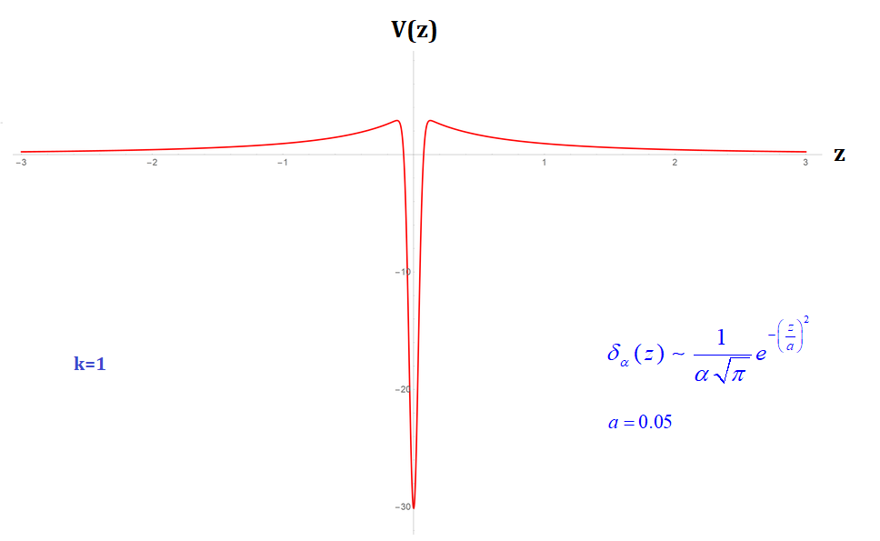
Figure 2.2: Qualitative graph of the function $V(z)$.

2.2.1 Kaluza-Klein Modes

The zero-mode $\psi_{0}(z)$ for $m_{0}=0$ can be easily evaluated from Eq.(2.80). Thus, it is

$$-\psi^{\prime\prime}_{0}(z)+\left[\frac{3}{2}A^{\prime\prime}(z)+\frac{9}{4}A^{\prime 2}(z)\right]\psi_{0}(z)=0\Rightarrow\psi_{0}(z)=N_{0}\ e^{\frac{3}{2}A(z)}\xRightarrow{\eqref{rs47}}$$

$$\psi_{0}(z)=N_{0}(k|z|+1)^{-3/2}$$ (2.85)

where $N_{0}$ is a normalization constant which is going to be evaluated followingly.

$$\int_{-L_{z}}^{L_{z}}dz\ |\psi_{0}(z)|^{2}=1\Rightarrow(N_{0})^{2}\int^{L_{z}}_{-L_{z}}dz(k|z|+1)^{-3}=2(N_{0})^{2}\int_{0}^{L_{z}}dz(kz+1)^{-3}=1\Rightarrow$$

$$(N_{0})^{2}\left[-\frac{1}{k(kL_{z}+1)^{2}}+\frac{1}{k}\right]=1\xRightarrow{kL_{z}=e^{kL}-1\gg 1}(N_{0})^{2}\frac{1}{k}=1\Rightarrow N_{0}=\sqrt{k}$$ (2.86)

From equations (2.85) and (2.86) we are led to

$$\boxed{\psi_{0}(z)=\frac{1}{k}\left(|z|+\frac{1}{k}\right)^{-3/2}}$$ (2.87)

The figure above depicts the plot of the potential $V(z)$ as it is given by equation (2.81), where it was used the approximation $\delta(z)\sim(1/a\sqrt{\pi})e^{-(z/a)^{2}}$ with $a=0.05$. This particular approximation helps us to visualize better the behaviour of the potential.

The boundary conditions are both satisfied. The figure in the next page depicts the plot of the graviton zero-mode at the region of the 3-brane which is located at $z=0$.

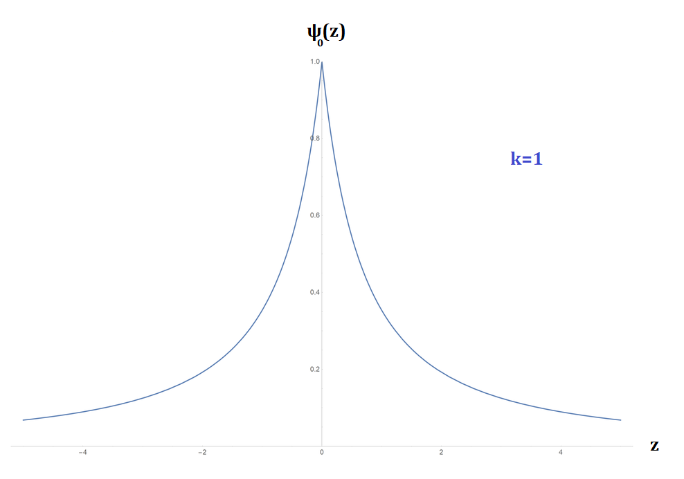
Figure 2.3: Qualitative graph of the zero-mode around the 3-brane at $z=0$.

The Kaluza-Klein (KK) modes for $n>0$ can be provided from the general equation (2.80).

$$\psi_{n}^{\prime\prime}(z)+\left[m_{n}^{2}-\frac{15k^{2}}{4(k|z|+1)^{2}}\right]\psi_{n}(z)=0$$ (2.88)

while for $z=0$ and $z=L_{z}$ equations (2.82) and (2.84) should be satisfied respectively. The above differential equation has the following general solution:

$$\psi_{n}(z)=\left(|z|+\frac{1}{k}\right)^{1/2}\left\{a_{n}J_{2}\left[m_{n}\left(|z|+\frac{1}{k}\right)\right]+b_{n}Y_{2}\left[m_{n}\left(|z|+\frac{1}{k}\right)\right]\right\}$$ (2.89)

where $a_{n}$, $b_{n}$ are constant coefficients and $J_{2}(z)$, $Y_{2}(z)$ are the Bessel functions of the first and second kind respectively. The derivative of the function $\psi_{n}(z)$ is given by

$$\psi_{n}^{\prime}(z)= m_{n}\left(|z|+\frac{1}{k}\right)^{1/2}\left\{a_{n}J_{1}\left[m_{n}\left(|z|+\frac{1}{k}\right)\right]+b_{n}Y_{1}\left[m_{n}\left(|z|+\frac{1}{k}\right)\right]\right\}$$

$$-\frac{3}{2}\left(|z|+\frac{1}{k}\right)^{-1/2}\left\{a_{n}J_{2}\left[m_{n}\left(|z|+\frac{1}{k}\right)\right]+b_{n}Y_{2}\left[m_{n}\left(|z|+\frac{1}{k}\right)\right]\right\}$$ (2.90)

We can relate the constants $a_{n}$ and $b_{n}$ by simply applying the boundary condition at $z=0$. Thus, from equations (2.82), (2.89) and (2.2.1) we get:

$$a_{n}=-b_{n}\frac{Y_{1}\left(\frac{m_{n}}{k}\right)}{J_{1}\left(\frac{m_{n}}{k}\right)}$$ (2.91)

Hence, it is:

$$\boxed{\psi_{n}(z)=N_{n}\left(|z|+\frac{1}{k}\right)^{1/2}\left\{-Y_{1}\left(\frac{m_{n}}{k}\right)J_{2}\left[m_{n}\left(|z|+\frac{1}{k}\right)\right]+J_{1}\left(\frac{m_{n}}{k}\right)Y_{2}\left[m_{n}\left(|z|+\frac{1}{k}\right)\right]\right\}}$$ (2.92)

where we defined

$$N_{n}=\frac{b_{n}}{J_{1}\left(\frac{m_{n}}{k}\right)}$$ (2.93)

Since the massless graviton mode is accompanied by a tower of massive Kaluza-Klein states, one may wonder about the gravitational potential that an observer on the visible brane will feel. In order to answer this, we will now consider each RS model separately.

The limit $\mathbold{m_{n}/k\gg 1}$

Combining equations (2.82), (2.84), (2.89) and (2.2.1) we get

$$a_{n}J_{1}\left(\frac{m_{n}}{k}\right)+b_{n}Y_{1}\left(\frac{m_{n}}{k}\right)=0$$ (2.94)

$$a_{n}J_{1}\left[m_{n}\left(L_{z}+\frac{1}{k}\right)\right]+b_{n}Y_{1}\left[m_{n}\left(L_{z}+\frac{1}{k}\right)\right]=0$$ (2.95)

It is well-known that a homogeneous system of equations in order to have a non-trivial solution it is necessary to have a vanishing determinant. Thus, for the previous system of equations we demand that

$$J_{1}\left(\frac{m_{n}}{k}\right)Y_{1}\left[m_{n}\left(L_{z}+\frac{1}{k}\right)\right]-J_{1}\left[m_{n}\left(L_{z}+\frac{1}{k}\right)\right]Y_{1}\left(\frac{m_{n}}{k}\right)=0\xRightarrow{kL_{z}=e^{kL}-1}$$

$$J_{1}\left(\frac{m_{n}}{k}\right)Y_{1}\left(\frac{m_{n}}{k}e^{kL}\right)-J_{1}\left(\frac{m_{n}}{k}e^{kL}\right)Y_{1}\left(\frac{m_{n}}{k}\right)=0$$ (2.96)

In this limit, the large value of the quantity $m_{n}/k$ results to the following expressions for the Bessel functions:

$$\left\{\begin{array}[]{cc}J_{1}\left(\frac{m_{n}}{k}\right)\sim\sqrt{\frac{2k}{\pi m_{n}}}\cos\left(\frac{m_{n}}{k}-\frac{3\pi}{4}\right),&\hskip 10.00002ptJ_{1}\left(\frac{m_{n}}{k}e^{kL}\right)\sim\sqrt{\frac{2k}{\pi m_{n}}e^{-kL}}\cos\left(\frac{m_{n}}{k}e^{kL}-\frac{3\pi}{4}\right)\\ \\ Y_{1}\left(\frac{m_{n}}{k}\right)\sim\sqrt{\frac{2k}{\pi m_{n}}}\sin\left(\frac{m_{n}}{k}-\frac{3\pi}{4}\right),&\hskip 10.00002ptY_{1}\left(\frac{m_{n}}{k}e^{kL}\right)\sim\sqrt{\frac{2k}{\pi m_{n}}e^{-kL}}\sin\left(\frac{m_{n}}{k}e^{kL}-\frac{3\pi}{4}\right)\end{array}\right\}$$ (2.97)

Therefore, Eq.(2.96) takes the form

$$\cos\left(\frac{m_{n}}{k}-\frac{3\pi}{4}\right)\sin\left(\frac{m_{n}}{k}e^{kL}-\frac{3\pi}{4}\right)-\cos\left(\frac{m_{n}}{k}e^{kL}-\frac{3\pi}{4}\right)\sin\left(\frac{m_{n}}{k}-\frac{3\pi}{4}\right)=0\Rightarrow$$

$$\sin\left[\frac{m_{n}}{k}\left(e^{kL}-1\right)\right]=0\xRightarrow{kL_{z}=e^{kL}-1}\sin\left(m_{n}L_{z}\right)=0\Rightarrow$$

$$\boxed{m_{n}=\frac{s\pi}{L_{z}},\hskip 10.00002pts=1,2,\ldots}$$ (2.98)

Correspondingly, Eq.(2.92) is given by

$$\psi_{n}(z)\sim N_{n}\sqrt{\frac{2k}{\pi m_{n}}}\sqrt{|z|+\frac{1}{k}} \left\{-\sin\left(\frac{m_{n}}{k}-\frac{3\pi}{4}\right)J_{2}\left[m_{n}\left(|z|+\frac{1}{k}\right)\right]\right.$$

$$\hskip 5.0pt\left.+\cos\left(\frac{m_{n}}{k}-\frac{3\pi}{4}\right)Y_{2}\left[m_{n}\left(|z|+\frac{1}{k}\right)\right]\right\}\xRightarrow{m_{n}(|z|+1/k)\gg 1}$$

$$\psi_{n}(z)\sim N_{n}\frac{2\sqrt{k}}{\pi m_{n}} \left\{-\sin\left(\frac{m_{n}}{k}-\frac{3\pi}{4}\right)\cos\left[m_{n}\left(|z|+\frac{1}{k}\right)-\frac{5\pi}{4}\right]\right.$$

$$\hskip 5.0pt\left.+\cos\left(\frac{m_{n}}{k}-\frac{3\pi}{4}\right)\sin\left[m_{n}\left(|z|+\frac{1}{k}\right)-\frac{5\pi}{4}\right]\right\}\Rightarrow$$

$$\psi_{n}(z)\sim N_{n}\frac{2\sqrt{k}}{\pi m_{n}}\sin\left(m_{n}|z|-\frac{\pi}{2}\right)$$ (2.99)

where we have used the following expressions for the Bessel function at the limit $m_{n}(|z|+1/k)\gg 1$.

$$\left(|z|+\frac{1}{k}\right)^{1/2}J_{2}\left[m_{n}\left(|z|+\frac{1}{k}\right)\right]\sim\sqrt{\frac{2}{\pi m_{n}}}\cos\left[m_{n}\left(|z|+\frac{1}{k}\right)-\frac{5\pi}{4}\right]$$ (2.100)

$$\left(|z|+\frac{1}{k}\right)^{1/2}Y_{2}\left[m_{n}\left(|z|+\frac{1}{k}\right)\right]\sim\sqrt{\frac{2}{\pi m_{n}}}\sin\left[m_{n}\left(|z|+\frac{1}{k}\right)-\frac{5\pi}{4}\right]$$ (2.101)

It is now trivial to evaluate the normalization constant $N_{n}$.

$$\int_{-L_{z}}^{L_{z}}dz\ \psi_{n}^{2}(z)=1\Rightarrow N_{n}^{2}\frac{4k}{\pi^{2}m_{n}^{2}}\int_{-L_{z}}^{L_{z}}dz\ \sin^{2}\left(m_{n}|z|-\frac{\pi}{2}\right)=1\Rightarrow$$

$$N_{n}^{2}\frac{4k}{\pi^{2}m_{n}^{2}}\ 2\ \underbrace{\int_{0}^{L_{z}}dz\ \sin^{2}\left(m_{n}z-\frac{\pi}{2}\right)}_{L_{z}/2\ (for\ L_{z}\gg 1)}=1\Rightarrow\boxed{N_{n}=\frac{\pi m_{n}}{2\sqrt{kL_{z}}}}$$ (2.102)

$$\eqref{rs94c}\xRightarrow{\eqref{rs94d}}\boxed{\psi_{n}(z)\sim\frac{1}{\sqrt{L_{z}}}\sin\left(m_{n}|z|-\frac{\pi}{2}\right)}$$ (2.103)

For the higher graviton modes to be very heavy, as assumed above, we should have a very small inter-brane distance according to Eq. (2.98). Then, this case applies to the RS1 model. Each graviton mode will contribute to the gravitational potential on the brane through a Yukawa-like potential, thus

$$U(r)\propto\sum_{n}\frac{G_{(4)}m_{1}m_{2}e^{-m_{n}r}}{r}$$

But since all the KK masses are very heavy, it is only the zero graviton that will create a $1/r$ potential while the contributions of the higher modes will be very much suppressed.

The limit $\mathbold{m_{n}/k\ll 1}$

At the approximation of $m_{n}/k\ll 1$, it is

$$J_{1}\left(\frac{m_{n}}{k}\right)\sim\frac{m_{n}}{2k},\hskip 30.00005ptY_{1}\left(\frac{m_{n}}{k}\right)\sim-\frac{2k}{\pi m_{n}}$$ (2.104)

Hence, we can safely state that $-Y_{1}\left(\frac{m_{n}}{k}\right)\gg J_{1}\left(\frac{m_{n}}{k}\right)$. Subsequently, Eq.(2.96) results to the following simple requirement in order to have a vanishing determinant:

$$J_{1}\left(\frac{m_{n}}{k}\ e^{kL}\right)=0\Rightarrow\boxed{m_{n}=ke^{-kL}R^{J_{1}}_{n}\simeq\frac{R^{J_{1}}_{n}}{L_{z}}}$$ (2.105)

where $R^{J_{1}}_{n}$ are the roots of the function $J_{1}(x)$, namely $J_{1}(R^{J_{1}}_{n})=0$. The masses $m_{n}$ of the massive graviton modes constitute the graviton spectrum (or Kaluza Klein spectrum). The substitution of the approximate relations from equation (2.104) into (2.92) leads to

$$\psi_{n}(z)\sim N_{n}\left(|z|+\frac{1}{k}\right)^{1/2}\left\{\frac{2k}{\pi m_{n}}J_{2}\left[m_{n}\left(|z|+\frac{1}{k}\right)\right]+\frac{m_{n}}{2k}Y_{2}\left[m_{n}\left(|z|+\frac{1}{k}\right)\right]\right\}\xRightarrow{N_{n}\rightarrow N_{n}\frac{m_{n}}{2k}}$$

$$\boxed{\psi_{n}(z)\sim N_{n}\left(|z|+\frac{1}{k}\right)^{1/2}\left\{\frac{4k^{2}}{\pi m_{n}^{2}}J_{2}\left[m_{n}\left(|z|+\frac{1}{k}\right)\right]+Y_{2}\left[m_{n}\left(|z|+\frac{1}{k}\right)\right]\right\}}$$ (2.106)

The normalization constant $N_{n}$ can be determined by the integral

$$\int_{-L_{z}}^{L_{z}}dz\ \psi_{n}^{2}(z)=1$$

The fact that $L_{z}\rightarrow\infty$ allows us to perform the calculation of $N_{n}$ in the approximation of $m_{n}|z|\gg 1$. Using also the fact that $\frac{m_{n}}{k}\ll 1\Rightarrow\frac{k}{m_{n}}\gg 1$, we can ignore the second term of Eq.(2.106) as negligible. Thus, the substitution of Eq.(2.100) into Eq.(2.106) leads to

$$\psi_{n}(z)\sim N_{n}\frac{4k^{2}}{\pi m_{n}^{2}}\sqrt{\frac{2}{\pi m_{n}}}\cos\left(m_{n}|z|-\frac{5\pi}{4}\right)$$ (2.107)

Thus, from Eq.(2.107) we have:

$$\int_{-L_{z}}^{L_{z}}dz\ \psi_{n}^{2}(z)=1\Rightarrow N^{2}_{n}\ \frac{32k^{4}}{\pi^{3}m^{5}_{n}}\int^{L_{z}}_{-L_{z}}\cos^{2}\left(m_{n}|z|-\frac{5\pi}{4}\right)=1\Rightarrow$$

$$N^{2}_{n}\ \frac{32k^{4}}{\pi^{3}m^{5}_{n}}\ 2\ \underbrace{\int^{L_{z}}_{0}\cos^{2}\left(m_{n}\ z-\frac{5\pi}{4}\right)}_{L_{z}/2\ \ (for\ L_{z}\gg 1)}=1\Rightarrow\boxed{N_{n}=\frac{\pi^{3/2}m_{n}^{5/2}}{4k^{2}\sqrt{2L_{z}}}}$$ (2.108)

Consequently, the graviton modes $\psi_{n}(z)$ for $n>0$ and $m_{n}|z|\gg 1$ are given by

$$\boxed{\psi_{n}(z)=\frac{1}{\sqrt{L_{z}}}\ \cos\left(m_{n}|z|-\frac{5\pi}{4}\right)}$$ (2.109)

In this case, the KK masses are assumed to be small and this can be realised only for a large inter-brane distance. Therefore, this analysis applies to the RS1 model, where resolving the hierarchy problem is not an objective any more, or to the RS2 model. Especially, in the latter case where $L\rightarrow\infty$, even the higher graviton modes become massless. It is thus even more important to verify if the Newtonian limit of gravity is indeed recovered on the visible brane. Here, the sum over the KK graviton states changes to an integral that must be carefully evaluated - we refer the interested reader to [42, 43] for more details on this. At the end, we present the result from [42] which is related to the gravitational potential that is generated by a massive object with mass $M$ on the 3-brane at $z=0$. The energy-momentum tensor for a point-mass at rest on the brane at $\vec{r}=0$ is the following:

$$T_{\mu\nu}=M\delta^{(3)}(\vec{r})\ \delta^{0}_{\mu}\ \delta^{0}_{\nu}$$

For $r=|\vec{r}|\gg 1/k$ we get:

$$h_{\mu\nu}=\frac{2G_{(5)}kM}{r}\left[\left(1+\frac{1}{3k^{2}r^{2}}\right)\eta_{\mu\nu}+\left(2+\frac{1}{k^{2}r^{2}}\right)\delta^{0}_{\mu}\delta^{0}_{\nu}\right]$$ (2.110)

Consequently, from equations (2.46) and (2.110) we obtain

$$h_{00}=\frac{2G_{(4)}M}{r}\left(1+\frac{2}{3k^{2}r^{2}}\right)$$ (2.111)

$$h_{ij}=\frac{2G_{(4)}M}{r}\left(1+\frac{1}{3k^{2}r^{2}}\right)\eta_{ij}$$ (2.112)

The gravitational potential $V(r)$ is given by $h_{00}$ as follows:

$$\boxed{V(r)=\frac{1}{2}h_{00}=\frac{G_{(4)}M}{r}\left(1+\frac{2}{3k^{2}r^{2}}\right)\xrightarrow{kr\gg 1}V(r)\sim\frac{G_{(4)}M}{r}}$$ (2.113)

Obviously, the desirable behaviour of an effective 4-dimensional gravity at the brane is produced by the model as $kr\gg 1$. On the other hand, if we consider the case of $kr\ll 1$, then the gravitational potential is proportional to $1/r^{2}$, i.e. $V(r)\propto 1/r^{2}$. This simply means that at short distances -compared to the scale $k$ which is also associated with the AdS curvature- gravity becomes 5-dimensional. The possibility to observe deviations from the Newton’s law of gravitation depends entirely on the value of $k$.

Chapter 3 Localization of a 5-Dimensional Brane-World Black Hole

The preceding analysis of RS models made clear that there is indeed a possibility to live at the boundaries of a higher dimensional cosmos (specifically a five-dimensional one) and the effective gravitational interaction between massive objects on our four-dimensional brane can be the same (in some limit) as the gravitational interaction which is provided by the established and well-tested gravitational theory of General Relativity. Hence, it is absolutely natural to wonder about the behaviour of 5-dimensional black holes in the context of RS models.

The first attempt to find a black hole solution in the aforementioned scenario was in [44]. The line-element which was considered is of the following form:

$$ds^{2}=e^{2A(y)}\left[-\left(1-\frac{2M}{r}\right)dt^{2}+\left(1-\frac{2M}{r}\right)^{-1}dr^{2}+r^{2}\left(d\theta^{2}+\sin^{2}\theta\ d\varphi^{2}\right)\right]+dy^{2}$$ (3.1)

where $M$ is a constant quantity and represents the mass of the black hole. As stated in the previous chapter, the coordinate $y$ is used for the extra dimension and $A(y)$ denotes the warp factor. For $A(y)=-k|y|$ we get the warp factor of the RS model. It is quite obvious that for $y=0$ the induced 4-dimensional line-element is identified with the well-known Schwarzschild spacetime geometry. However, a 5-dimensional observer will not be able to associate the complete 5-dimensional line-element of Eq.(3.1) with a regular black hole. The previous statement can be easily verified by the Kretschmann scalar $K\equiv R_{MNKL}R^{MNKL}$ that emanates from the line-element (3.1).

$$K\equiv R_{MNKL}R^{MNKL}=8\left[2A^{\prime\prime}(y)^{2}+5A^{\prime}(y)^{4}+4A^{\prime}(y)^{2}A^{\prime\prime}(y)+\frac{6M^{2}e^{-4A(y)}}{r^{6}}\right]$$ (3.2)

The last term of Eq.(3.2) reveals the existence of a singularity at $r=0$ which extends from $-\infty$ to $+\infty$ along the extra dimension $y$. Hence, the line-element of Eq.(3.1) generates a black string rather than a black hole. Of course, for any descending function $A(y)$ the last term of Eq.(3.2) becomes even more problematic, because when $y\rightarrow\infty$ the quantity $e^{-4A(y)}$ goes to infinity as well. This particular behaviour is in complete contrast to the purpose of the RS model, which intends to keep gravity localized near the brane at $y=0$.

There is a plethora of attempts in the literature that try to derive a 5-dimensional black hole which is localized close to the brane (we mention some of them: [45, 46, 47, 48, 49, 50, 51, 52, 53, 54, 55, 36]. Additionally, there are numerical solutions which describe both mini and large brane-world black holes in the context of RS models and beyond (i.e. 6-dimensional black holes) [56, 57, 58, 59]. However, an analytical solution which can be written in closed form has not been found, thus, the investigation of such a solution is still incomplete. Finally, it is important to refer that in [60, 61, 62] black hole solutions were found which are localized on a 2-brane embedded in a (3+1)-dimensional bulk. Therefore, the motivation to search for a corresponding solution for the higher dimensional problem (3-brane in a (4+1)-dimensional bulk) is completely justified.

This Chapter and the rest of the thesis is entirely focused on the examination of the existence of a localized black hole solution in the context of a brane-world model which is similar to the RS2 model. The word “similar” was used because the warp factor $A(y)$ is allowed to differ from the expression $-k|y|$ (but it is necessary to be a descending function, as it is in the RS models) in order to increase the chances of finding a localized 5-dimensional black hole solution. In the following section we present the geometrical background that is going to be used in the framework of this thesis.

3.1 The Geometry of the 5-Dimensional Spacetime

We assume that the 4-dimensional part of the general 5-dimensional geometrical background is a Vaidya metric. We also consider that mass is a function of three variables $m=m(v,r,y)$ (motivated by [36]). The non-trivial dependence of the mass from the extra dimension $y$ is needed in order to counter the anomalous effect of the quantity $e^{-4A(y)}$ in the last term of equation (3.2). An appropriate mass function that decreases faster than $e^{-4A(y)}$ increases and has also the necessary r-dependence in order to describe a black hole, would solve the localization problem. The drawback of this non-trivial assumption of the mass parameter is that it demands the existence of a bulk matter distribution in order to get consistent field equations. The bulk matter distribution that it is going to be considered in the context of this thesis will be presented later in this Chapter. Thus, the line element is of the form

$$ds^{2}=e^{2A(y)}\left[-\left(1-\frac{2m(v,r,y)}{r}\right)dv^{2}+2dvdr+r^{2}(d\theta^{2}+\sin^{2}\theta\ d\varphi^{2})\right]+dy^{2}$$ (3.3)

It is easily deducible that the covariant components of the metric tensor in matrix form are:

$$(g_{MN})=\left(\begin{array}[]{ccccc}-e^{2A(y)}\left(1-\frac{2m(u,r,y)}{r}\right)&e^{2A(y)}&0&0&0\\ e^{2A(y)}&0&0&0&0\\ 0&0&e^{2A(y)}r^{2}&0&0\\ 0&0&0&e^{2A(y)}r^{2}\sin^{2}(\theta)&0\\ 0&0&0&0&1\\ \end{array}\right)$$ (3.4)

Thus, the contravariant components of the metric tensor are of the following form:

$$(g^{MN})=\left(\begin{array}[]{ccccc}0&e^{-2A(y)}&0&0&0\\ e^{-2A(y)}&e^{-2A(y)}\left(1-\frac{2m(u,r,y)}{r}\right)&0&0&0\\ 0&0&\frac{e^{-2A(y)}}{r^{2}}&0&0\\ 0&0&0&\frac{e^{-2A(y)}}{r^{2}\sin^{2}\theta}&0\\ 0&0&0&0&1\\ \end{array}\right)$$ (3.5)

For the metric ansatz (3.3), the quantities that are invariant and also contain the complete information of the 5-dimensional curvature, are $R=g_{MN}R^{MN}$, $R_{MN}R^{MN}$ and $R_{ABCD}R^{ABCD}$. As it is mentioned earlier, an acceptable solution for the mass function $m=m(v,r,y)$ should have an appropriate dependence on the y-coordinate in order to expunge any singularities in the bulk. Hence, the desirable solution should yield to a regular Anti-de Sitter space-time at a finite distance from the brane and a 5-dimensional black hole localized on the brane, otherwise the solution is rejected.

The Christoffel symbols can be evaluated with the use of equations (3.4), (3.5) and the following relation:

$$\Gamma^{K}{}_{MN}=\frac{1}{2}g^{KL}\left(g_{ML,N}+g_{NL,M}-g_{MN,L}\right)$$ (3.6)

In the table that follows are depicted the non-zero Christoffel symbols.

$$\begin{array}[]{ccc}\Gamma^{0}{}_{00}=\frac{m-r\partial_{r}m}{r^{2}}&\Gamma^{0}{}_{04}=\Gamma^{0}{}_{40}=A^{\prime}&\Gamma^{0}{}_{22}=-r\\ \\ \Gamma^{0}{}_{33}=-r\sin^{2}\theta&\Gamma^{1}{}_{00}=\frac{r^{2}\partial_{v}m-(r-2m)\left(r\partial_{r}m-m\right)}{r^{3}}&\Gamma^{1}{}_{01}=\Gamma^{1}{}_{10}=\frac{r\partial_{r}m-m}{r^{2}}\\ \\ \Gamma^{1}{}_{04}=\Gamma^{1}{}_{40}=\frac{\partial_{y}m}{r}&\Gamma^{1}{}_{14}=\Gamma^{1}{}_{41}=A^{\prime}&\Gamma^{1}{}_{22}=2m-r\\ \\ \Gamma^{1}{}_{33}=(2m-r)\sin^{2}\theta&\Gamma^{2}{}_{12}=\Gamma^{2}{}_{21}=\frac{1}{r}&\Gamma^{2}{}_{24}=\Gamma^{2}{}_{42}=A^{\prime}\\ \\ \Gamma^{2}{}_{33}=-\sin\theta\cos\theta&\Gamma^{3}{}_{13}=\Gamma^{3}{}_{31}=\frac{1}{r}&\Gamma^{3}{}_{23}=\Gamma^{3}{}_{32}=\cot\theta\\ \\ \Gamma^{3}{}_{34}=\Gamma^{3}{}_{43}=A^{\prime}&\Gamma^{4}{}_{00}=\frac{e^{2A}\left(A^{\prime}(r-2m)-\partial_{y}m\right)}{r}&\Gamma^{4}{}_{01}=\Gamma^{4}{}_{10}=-e^{2A}A^{\prime}\\ \\ \Gamma^{4}{}_{22}=-r^{2}e^{2A}A^{\prime}&\Gamma^{4}{}_{33}=-r^{2}A^{\prime}e^{2A}\sin^{2}\theta&\end{array}$$ (3.7)

Subsequently, we present the 5-dimensional curvature invariant quantities.

$$R=R_{MN}g^{MN}=-20A^{\prime 2}-8A^{\prime\prime}+\frac{2e^{-2A}}{r}\left(\partial_{r}^{2}m+\frac{2\partial_{r}m}{r}\right)$$ (3.8)

$$\begin{array}[]{l}R_{MN}R^{MN}=80A^{\prime 2}+64A^{\prime 2}A^{\prime\prime}+20A^{\prime\prime 2}-\displaystyle{\frac{4e^{-2A}}{r}}\left(\partial_{r}^{2}m+\frac{2\partial_{r}m}{r}\right)(4A^{\prime 2}+A^{\prime\prime})\\ \hskip 50.00008pt+\displaystyle{\frac{2e^{-4A}}{r^{2}}}\left[(\partial_{r}^{2}m)^{2}+\frac{4(\partial_{r}m)^{2}}{r^{2}}\right]\end{array}$$ (3.9)

$$\begin{array}[]{c}\scriptstyle{R^{ABCD}R_{ABCD}}=\scriptstyle{40A^{\prime 4}+32A^{\prime 2}A^{\prime\prime}+16A^{\prime\prime 2}+}\scriptstyle{\frac{48e^{-4A}m^{2}}{r^{6}}}-\frac{8e^{-2A}A^{\prime 2}}{r}\left(\partial_{r}^{2}m+\frac{2\partial_{r}m}{r}\right)\\ \\ \hskip 60.00009pt\scriptstyle{+\frac{4e^{-4A}}{r^{2}}}\left[(\partial_{r}^{2}m)^{2}+\frac{4m}{r^{2}}\left(\partial_{r}^{2}m-\frac{4\partial_{r}m}{r}\right)-\frac{4\partial_{r}m\partial_{r}^{2}m}{r}+\frac{8(\partial_{r}m)^{2}}{r}\right]\end{array}$$ (3.10)

The non-zero covariant components of the Einstein tensor $G_{MN}$ are:

$$\begin{array}[]{c}G_{00}=\frac{-e^{2A}\left[3(r-2m)\left(2A^{\prime 2}+A^{\prime\prime}\right)+4A^{\prime}\partial_{y}m+\partial_{y}^{2}m\right]r^{2}+2r\partial_{v}m+2(r-2m)\partial_{r}m}{r^{3}}\\ \\ G_{01}=G_{10}=\displaystyle{3e^{2A}\left(2A^{\prime 2}+A^{\prime\prime}\right)-\frac{2\partial_{r}m}{r^{2}}}\\ \\ G_{04}=G_{40}=\displaystyle{\frac{\partial_{y}m+r\partial_{r}\partial_{y}m}{r^{2}}}\\ \\ G_{22}=\displaystyle{r\left[3e^{2A}r\left(2A^{\prime 2}+A^{\prime\prime}\right)-\partial_{r}^{2}m\right]}\\ \\ G_{33}=\displaystyle{r\sin^{2}\theta\left[3e^{2A}r\left(2A^{\prime 2}+A^{\prime\prime}\right)-\partial_{r}^{2}m\right]}\\ \\ G_{44}=\displaystyle{6A^{\prime 2}-\frac{e^{-2A}\left(2\partial_{r}m+r\partial_{r}^{2}m\right)}{r^{2}}}\end{array}$$ (3.11)

while the mixed components of the Einstein tensor $G^{M}{}_{N}=g^{MK}G_{KN}$ are the following:

$$\begin{array}[]{c}G^{0}{}_{0}=\displaystyle{6A^{\prime 2}+3A^{\prime\prime}-\frac{2e^{-2A}\partial_{r}m}{r^{2}}}\\ \\ G^{1}{}_{0}=\displaystyle{-\frac{4rA^{\prime}\partial_{y}m+r\partial_{y}^{2}m-2e^{-2A}\partial_{v}m}{r^{2}}}\\ \\ G^{1}{}_{1}=\displaystyle{6A^{\prime 2}+3A^{\prime\prime}-\frac{2e^{-2A}\partial_{r}m}{r^{2}}}\\ \\ G^{1}{}_{4}=\displaystyle{\frac{e^{-2A}\left(\partial_{y}m+r\partial_{r}\partial_{y}m\right)}{r^{2}}}\\ \\ G^{2}{}_{2}=\displaystyle{6A^{\prime 2}+3A^{\prime\prime}-\frac{e^{-2A}\partial_{r}^{2}m}{r}}\\ \\ G^{3}{}_{3}=\displaystyle{6A^{\prime 2}+3A^{\prime\prime}-\frac{e^{-2A}\partial_{r}^{2}m}{r}}\\ \\ G^{4}{}_{0}=\displaystyle{\frac{\partial_{y}m+r\partial_{r}\partial_{y}m}{r^{2}}}\\ \\ G^{4}{}_{4}=\displaystyle{6A^{\prime 2}-\frac{e^{-2A}\left(2\partial_{r}m+r\partial_{r}^{2}m\right)}{r^{2}}}\end{array}$$ (3.12)

A detailed presentation of all the geometrical quantities i.e. Christoffel symbols, Riemann tensor, Ricci tensor and Einstein tensor, takes place in Appendix E. Moreover, in the same Chapter of Appendices, one can find the proper mathematica commands in order to verify the validity of all the aforementioned quantities.

In the following section, we introduce the field theory model in the context of which the existence of a viable solution to the localization problem of a 5-dimensional black hole will be examined.

3.2 Two Non-Minimally Coupled and Interacting Scalar Fields

We consider the most general case of two interacting scalar fields $\phi,\chi$ which are not minimally coupled to gravity. These scalar fields can freely propagate into the bulk. Subsequently, the action of this model is the following:

$$S=\int d^{4}xdy\sqrt{-g^{(5)}}\left[\frac{f(\phi,\chi)}{2\kappa_{(5)}}R-\frac{1}{2}(\nabla\phi)^{2}-\frac{1}{2}(\nabla\chi)^{2}-V(\phi,\chi)-\Lambda_{B}\right]$$ (3.13)

where $g^{(5)}=\det[(g_{MN})]$. The scalar fields $\phi$, $\chi$ are both functions of the variables $(v,r,y)$ and $\Lambda_{B}$ denotes the cosmological constant of the bulk, it is the same constant as $\Lambda_{5}$ which was used in Chapter 2. The field equations of this model can be derived by varying the action with respect to the metric tensor and also with respect to the fields $\phi,\chi$. The steps that are going to be followed for the variation of the above action are the same as the steps which are followed in Appendix F, where it is thoroughly presented the variation of a single scalar field which is non-minimally coupled to gravity. Thus, we have:

$$\delta S=0 =\int d^{4}xdy\ \delta\left(\sqrt{-g^{(5)}}\right)\left[\frac{f(\phi,\chi)}{2\kappa_{(5)}}R-\frac{1}{2}(\nabla\phi)^{2}-\frac{1}{2}(\nabla\chi)^{2}-V(\phi,\chi)-\Lambda_{B}\right]$$

$$\ \ \ \ +\int d^{4}xdy\sqrt{-g^{(5)}}\left\{\frac{f(\phi,\chi)}{2\kappa_{(5)}}\delta R-\frac{1}{2}\delta[(\nabla\phi)^{2}]-\frac{1}{2}\delta[(\nabla\chi)^{2}]\right\}$$ (3.14)

Moreover, it is

$$\delta[(\nabla\phi)^{2}]=\delta(\nabla^{M}\phi\nabla_{M}\phi)=\delta(g^{MN}\nabla_{M}\phi\nabla_{N}\phi)=\nabla_{M}\phi\nabla_{N}\phi\ \delta g^{MN}$$ (3.15)

Using equations (3.15), (• ‣ F.1), (F.28) and (F.41) into (3.2) we get:

$$0 =\int d^{4}xdy\sqrt{-g^{(5)}}\ \delta g^{MN}\left\{-\frac{1}{2}g_{MN}\left[\frac{f(\phi,\chi)}{2\kappa_{(5)}}R-\frac{1}{2}(\nabla\phi)^{2}-\frac{1}{2}(\nabla\chi)^{2}-V(\phi,\chi)-\Lambda_{B}\right]\right.$$

$$\ \ \ \ \left.+\frac{1}{2\kappa_{(5)}}f(\phi,\chi)R_{MN}-\frac{1}{2}\nabla_{M}\nabla_{N}f(\phi,\chi)+\frac{1}{2}g_{MN}\square f(\phi,\chi)-\frac{1}{2}\nabla_{M}\phi\nabla_{N}\phi-\frac{1}{2}\nabla_{M}\chi\nabla_{N}\chi\right\}\Rightarrow$$

$$0 =\frac{f(\phi,\chi)}{\kappa_{(5)}}\left(R_{MN}-\frac{1}{2}g_{MN}R\right)+g_{MN}\left[\frac{(\nabla\phi)^{2}}{2}+\frac{(\nabla\chi)^{2}}{2}+V(\phi,\chi)\right]+g_{MN}\Lambda_{B}-\nabla_{M}\phi\nabla_{N}\phi$$

$$\ \ \ \ -\nabla_{M}\chi\nabla_{N}\chi-\nabla_{M}\nabla_{N}f(\phi,\chi)+g_{MN}\square f(\phi,\chi)\Rightarrow$$

$$\boxed{f(\phi,\chi)\left(R_{MN}-\frac{1}{2}g_{MN}R\right)=f(\phi,\chi)\ G_{MN}=\kappa_{(5)}\left(T_{MN}-g_{MN}\Lambda_{B}\right)}$$ (3.16)

where

$$\boxed{T_{MN}=\nabla_{M}\phi\nabla_{N}\phi+\nabla_{M}\chi\nabla_{N}\chi-g_{MN}\left[\frac{(\nabla\phi)^{2}}{2}+\frac{(\nabla\chi)^{2}}{2}+V\right]+\nabla_{M}\nabla_{N}f-g_{MN}\square f}$$ (3.17)

The above field equations are more convenient for calculations when they are expressed in terms of mixed tensor components. Hence, we have

$$f(\phi,\chi)\ G^{M}{}_{N}=T^{M}{}_{N}-\delta^{M}{}_{N}\Lambda_{B}$$ (3.18)

where we have absorbed the constant $\kappa_{(5)}$ inside the function $f(\phi,\chi)$ and

$$\begin{array}[]{l}T^{M}{}_{N}=\nabla^{M}\phi\nabla_{N}\phi+\nabla^{M}\chi\nabla_{N}\chi-\delta^{M}{}_{N}\left[\frac{(\nabla\phi)^{2}}{2}+\frac{(\nabla\chi)^{2}}{2}+V\right]+\nabla^{M}\nabla_{N}f-\delta^{M}{}_{N}\square f\\ \\ \hskip 25.50006pt=\partial^{M}\phi\partial_{N}\phi+\partial^{M}\chi\partial_{N}\chi-\delta^{M}{}_{N}\left[\frac{(\partial\phi)^{2}}{2}+\frac{(\partial\chi)^{2}}{2}+V\right]+\nabla^{M}\nabla_{N}f-\delta^{M}{}_{N}\square f\end{array}$$ (3.19)

The variation of the action (3.13) with respect to the fields $\phi,\chi$ (as it is done in the second section of Appendix F) provides us with two additional equations that should be satisfied in order to have an acceptable solution for the mass function and the scalar fields. In complete analogy to the variation method of section F.2, it is straightforward to derive the following expressions:

$$\sqrt{-g^{(5)}}\left(\frac{1}{2}\frac{\partial f}{\partial\phi}R-\frac{\partial V}{\partial\phi}\right)=-\partial_{M}\left(\sqrt{-g^{(5)}}\ g^{MN}\partial_{N}\phi\right)$$ (3.20)

$$\sqrt{-g^{(5)}}\left(\frac{1}{2}\frac{\partial f}{\partial\chi}R-\frac{\partial V}{\partial\chi}\right)=-\partial_{M}\left(\sqrt{-g^{(5)}}\ g^{MN}\partial_{N}\chi\right)$$ (3.21)

In order to derive the independent field equations that are resulting from relations (3.18) and (3.19) we firstly need to evaluate the mixed components of the energy-momentum tensor $T^{M}{}_{N}$. In Appendix G there is a comprehensive evaluation of the components of the energy-momentum tensor given by Eq.(3.19), thus, it is redundant to repeat any of these calculations. Subsequently, the non-zero components of the energy-momentum tensor are depicted in their compact form.

$$T^{0}{}_{1} =e^{-2A}[(\partial_{1}\phi)^{2}+(\partial_{1}\chi)^{2}+\partial_{1}^{2}f]$$

$$T^{1}{}_{0} =e^{-2A}\left[(\partial_{0}\phi)^{2}+(\partial_{0}\chi)^{2}+\partial_{0}^{2}f+\left(1-\frac{2m}{r}\right)(\partial_{1}\partial_{0}\phi+\partial_{1}\chi\partial_{0}\chi+\partial_{1}\partial_{0}f)\right.$$

$$\hskip 50.00008pt\left.+\partial_{1}\left(\frac{m}{r}\right)\partial_{0}f-\partial_{0}\left(\frac{m}{r}\right)\partial_{1}f+e^{2A}\partial_{4}\left(\frac{m}{r}\right)\partial_{4}f\right]$$

$$T^{4}{}_{0} =\partial_{4}\phi\partial_{0}\phi+\partial_{4}\chi\partial_{0}\chi+\partial_{4}\partial_{0}f-A^{\prime}\partial_{0}f-\frac{\partial_{4}m}{r}\partial_{1}f$$

$$T^{0}{}_{4} =e^{-2A}(\partial_{1}\phi\partial_{4}\phi+\partial_{1}\chi\partial_{4}\chi+\partial_{1}\partial_{4}f-A^{\prime}\partial_{1}f)$$

$$T^{4}{}_{1} =e^{2A}T^{0}{}_{4}$$

$$T^{1}{}_{4} =e^{-2A}T^{4}{}_{0}+\left(1-\frac{2m}{r}\right)T^{0}{}_{4}$$

$$T^{0}{}_{0} =e^{-2A}\left[\partial_{1}\phi\partial_{0}\phi+\partial_{1}\chi\partial_{0}\chi+\partial_{1}\partial_{0}f-\partial_{1}\left(\frac{m}{r}\right)\partial_{1}f\right]+A^{\prime}\partial_{4}f+\mathcal{L}-\square f$$ (3.22)

$$T^{1}{}_{1} =T^{0}{}_{0}+\left(1-\frac{2m}{r}\right)T^{0}{}_{1}$$

$$T^{2}{}_{2} =\frac{e^{-2A}}{r}\left[\partial_{0}f+\left(1-\frac{2m}{r}\right)\partial_{1}f\right]+A^{\prime}\partial_{4}f+\mathcal{L}-\square f$$

$$T^{3}{}_{3} =T^{2}{}_{2}$$

$$T^{4}{}_{4} =(\partial_{4}\phi)^{2}+(\partial_{4}\chi)^{2}+\partial^{2}_{4}f+\mathcal{L}-\square f$$

$$\mathcal{L} =-\frac{e^{-2A}}{2}\left\{2(\partial_{1}\phi\partial_{0}\phi+\partial_{1}\chi\partial_{0}\chi)+\left(1-\frac{2m}{r}\right)[(\partial_{1}\phi)^{2}+(\partial_{1}\chi)^{2}]\right\}$$

$$\hskip 50.00008pt-\frac{1}{2}[(\partial_{4}\phi)^{2}+(\partial_{4}\chi)^{2}]-V(\phi,\chi)$$

$$\square f =e^{-2A}\partial_{0}\partial_{1}f+\frac{e^{-2A}}{r^{2}}\partial_{1}\left[r^{2}\partial_{0}f+r^{2}\left(1-\frac{2m}{r}\right)\partial_{1}f\right]+e^{-4A}\partial_{4}\left(e^{4A}\partial_{4}f\right)$$

3.3 The Field Equations of the Theory

Having in our disposal both the components of the Einstein tensor from equation (3.12) and the components of the energy-momentum tensor given by equation (3.2), the independent field equations can immediately ensue with the use of equation (3.18). It is clear that the independent field equations are the following.

Equation $(^{0}{}_{1})$:

$$\eqref{loc.14}\xRightarrow[\eqref{loc.93}]{\eqref{loc.7}}(\partial_{1}\phi)^{2}+(\partial_{1}\chi)^{2}+\partial_{1}^{2}f=0$$ (3.23)

Substituting $\partial_{1}^{2}f$ from equation (G) into (3.23) we get

$$(1+\partial_{\phi}^{2}f)(\partial_{1}\phi)^{2}+(1+\partial_{\chi}^{2}f)(\partial_{1}\chi)^{2}+2\partial_{\chi}\partial_{\phi}f\partial_{1}\chi\partial_{1}\phi+\partial_{\phi}f\partial_{1}^{2}\phi+\partial_{\chi}f\partial_{1}^{2}\chi=0$$ (3.24)

Equation $(^{1}{}_{0})$:

$$\eqref{loc.14}\xRightarrow[\eqref{loc.93}]{\eqref{loc.7}}(\partial_{0}\phi)^{2}+(\partial_{0}\chi)^{2}+\partial_{0}^{2}f+\left(1-\frac{2m}{r}\right)(\partial_{1}\phi\partial_{0}\phi+\partial_{1}\chi\partial_{0}\chi+\partial_{1}\partial_{0}f)+\partial_{1}\left(\frac{m}{r}\right)\partial_{0}f$$

$$-\partial_{0}\left(\frac{m}{r}\right)\partial_{1}f+e^{2A}\partial_{4}\left(\frac{m}{r}\right)\partial_{4}f=f\left[\frac{2}{r^{2}}\partial_{0}m-\frac{e^{2A}}{r}(\partial_{4}^{2}m+4A^{\prime}\partial_{4}m)\right]$$ (3.25)

The substitution of quantities $\partial_{0}^{2}f$ and $\partial_{1}\partial_{0}f$ from equations (G) and (G) respectively into equation (3.25) yields to

$$e^{-2A}\left\{(1+\partial_{\phi}^{2}f)(\partial_{0}\phi)^{2}+(1+\partial_{\chi}^{2}f)(\partial_{0}\chi)^{2}+2\partial_{\chi}\partial_{\phi}f\partial_{0}\phi\partial_{0}\chi+\partial_{\phi}f\partial_{0}^{2}\phi+\partial_{\chi}f\partial_{0}^{2}\chi\right.$$

$$\hskip 20.00003pt+\left(1-\frac{2m}{r}\right)[(1+\partial_{\phi}^{2}f)\partial_{1}\phi\partial_{0}\phi+(1+\partial_{\chi}^{2}f)\partial_{1}\chi\partial_{0}\chi+\partial_{\phi}\partial_{\chi}f(\partial_{1}\phi\partial_{0}\chi+\partial_{1}\chi\partial_{0}\phi)+\partial_{\phi}f\partial_{1}\partial_{0}\phi+\partial_{\chi}f\partial_{1}\partial_{0}\chi]$$

$$\left.+\left(\frac{\partial_{1}m}{r}-\frac{m}{r^{2}}\right)(\partial_{\phi}f\partial_{0}\phi+\partial_{\chi}f\partial_{0}\chi)-\frac{\partial_{0}m}{r}(\partial_{\phi}f\partial_{1}\phi+\partial_{\chi}f\partial_{1}\chi)+e^{2A}\frac{\partial_{4}m}{r}(\partial_{\phi}f\partial_{4}\phi+\partial_{\chi}f\partial_{4}\chi)\right\}=$$

$$=f\left[\frac{2}{r^{2}}\partial_{0}m-\frac{e^{2A}}{r}(\partial_{4}^{2}m+4A^{\prime}\partial_{4}m)\right]$$ (3.26)

Equation $(^{4}{}_{0})$:

$$\eqref{loc.14}\xRightarrow[\eqref{loc.93}]{\eqref{loc.7}}\partial_{4}\phi\partial_{0}\phi+\partial_{4}\chi\partial_{0}\chi+\partial_{4}\partial_{0}f-A^{\prime}\partial_{0}f-\frac{\partial_{4}m}{r}\partial_{1}f=\frac{f}{r}\left(\frac{\partial_{4}m}{r}+\partial_{1}\partial_{4}m\right)$$ (3.27)

The last equation in its extended form is:

$$(1+\partial_{\phi}^{2}f)\partial_{4}\phi\partial_{0}\phi+(1+\partial_{\chi}^{2}f)\partial_{4}\chi\partial_{0}\chi+\partial_{\chi}\partial_{\phi}f(\partial_{4}\chi\partial_{0}\phi+\partial_{4}\phi\partial_{0}\chi)+\partial_{\phi}f\partial_{4}\partial_{0}\phi+\partial_{\chi}f\partial_{4}\partial_{0}\chi$$

$$-A^{\prime}\partial_{0}f-\frac{\partial_{4}m}{r}(\partial_{\phi}f\partial_{1}\phi+\partial_{\chi}f\partial_{1}\chi)=\frac{f}{r}\left(\frac{\partial_{4}m}{r}+\partial_{1}\partial_{4}m\right)$$ (3.28)

Equation $(^{0}{}_{4})$:

$$\eqref{loc.14}\xRightarrow[\eqref{loc.93}]{\eqref{loc.7}}\partial_{1}\phi\partial_{4}\phi+\partial_{1}\chi\partial_{4}\chi+\partial_{1}\partial_{4}f-A^{\prime}\partial_{1}f=0$$ (3.29)

Using equation (G) into equation (3.29) we obtain

$$(1+\partial_{\phi}^{2}f)\partial_{1}\phi\partial_{4}\phi+(1+\partial_{\chi}^{2}f)\partial_{1}\chi\partial_{4}\chi+\partial_{\phi}\partial_{\chi}f(\partial_{1}\chi\partial_{4}\phi+\partial_{1}\phi\partial_{4}\chi)+\partial_{\phi}f\partial_{1}\partial_{4}\phi$$

$$+\partial_{\chi}f\partial_{1}\partial_{4}\chi-A^{\prime}(\partial_{\phi}f\partial_{1}\phi+\partial_{\chi}f\partial_{1}\chi)=0$$ (3.30)

Equation $(^{0}{}_{0})$:

$$\eqref{loc.14}\xRightarrow[\eqref{loc.93}]{\eqref{loc.7}}e^{-2A}\left[\partial_{1}\phi\partial_{0}\phi+\partial_{1}\chi\partial_{0}\chi+\partial_{1}\partial_{0}f-\partial_{1}\left(\frac{m}{r}\right)\partial_{1}f\right]+A^{\prime}\partial_{4}f+\mathcal{L}-\square f-\Lambda_{B}=$$

$$=f\left(6A^{\prime 2}+3A^{\prime\prime}-\frac{2e^{-2A}}{r^{2}}\partial_{1}m\right)$$ (3.31)

Equation (3.31) is equivalent to

$$e^{-2A}\left[(1+\partial_{\phi}^{2}f)\partial_{1}\phi\partial_{0}\phi+(1+\partial_{\chi}^{2}f)\partial_{1}\chi\partial_{0}\chi+\partial_{\chi}\partial_{\phi}f(\partial_{1}\chi\partial_{0}\phi+\partial_{1}\phi\partial_{0}\chi)+\partial_{\phi}f\partial_{1}\partial_{0}\phi+\partial_{\chi}f\partial_{1}\partial_{0}\chi\right.$$

$$\left.+\frac{\partial_{\phi}f\partial_{1}\phi+\partial_{\chi}f\partial_{1}\chi}{r}\left(\frac{m}{r}-\partial_{1}m\right)\right]+A^{\prime}(\partial_{\phi}f\partial_{4}\phi+\partial_{\chi}f\partial_{4}\chi)+\mathcal{L}-\square f-\Lambda_{B}=$$

$$=f\left(6A^{\prime 2}+3A^{\prime\prime}-\frac{2e^{-2A}}{r^{2}}\partial_{1}m\right)$$ (3.32)

Equation $(^{2}{}_{2})$:

$$\eqref{loc.14}\xRightarrow[\eqref{loc.93}]{\eqref{loc.7}}\frac{e^{-2A}}{r}\left[\partial_{0}f+\left(1-\frac{2m}{r}\right)\partial_{1}f\right]+A^{\prime}\partial_{4}f+\mathcal{L}-\square f-\Lambda_{B}=$$

$$=f\left(6A^{\prime 2}+3A^{\prime\prime}-\frac{e^{-2A}}{r}\partial_{1}^{2}m\right)$$ (3.33)

Expanding the partial derivatives of the function $f=f(\phi,\chi)$ we get

$$\frac{e^{-2A}}{r}\left[(\partial_{\phi}f\partial_{0}\phi+\partial_{\chi}f\partial_{0}\chi)+\left(1-\frac{2m}{r}\right)(\partial_{\phi}f\partial_{1}\phi+\partial_{\chi}f\partial_{1}\chi)\right]+A^{\prime}(\partial_{\phi}f\partial_{4}\phi+\partial_{\chi}f\partial_{4}\chi)$$

$$+\mathcal{L}-\square f-\Lambda_{B}=f\left(6A^{\prime 2}+3A^{\prime\prime}-\frac{e^{-2A}}{r}\partial_{1}^{2}m\right)$$ (3.34)

Equation $(^{4}{}_{4})$:

$$\eqref{loc.14}\xRightarrow[\eqref{loc.93}]{\eqref{loc.7}}(\partial_{4}\phi)^{2}+(\partial_{4}\chi)^{2}+\partial^{2}_{4}f+\mathcal{L}-\square f-\Lambda_{B}=f\left(6A^{\prime 2}-\frac{e^{-2A}}{r}\partial_{1}^{2}m-\frac{2e^{-2A}}{r^{2}}\partial_{1}m\right)$$ (3.35)

The combination of equations (G) and (3.35) gives

$$(1+\partial_{\phi}^{2}f)(\partial_{4}\phi)^{2}+(1+\partial_{\chi}^{2}f)(\partial_{4}\chi)^{2}+2\partial_{\chi}\partial_{\phi}f\partial_{4}\chi\partial_{4}\phi+\partial_{\phi}f\partial_{4}^{2}\phi+\partial_{\chi}f\partial_{4}^{2}\chi+\mathcal{L}-\square f-\Lambda_{B}=$$

$$=f\left(6A^{\prime 2}-\frac{e^{-2A}}{r}\partial_{1}^{2}m-\frac{2e^{-2A}}{r^{2}}\partial_{1}m\right)$$ (3.36)

Instead of using equations (3.31), (3.33), (3.35) and the corresponding extended equations (3.32), (3.34) and (3.36), which contain the terms $\mathcal{L}$ and $\square f$ that add extra complexity, we can be exempted from these terms by combining the aforementioned equations with each other.

Equation $(^{0}{}_{0})-$Equation $(^{2}{}_{2})$:

Subtracting equation (3.33) from (3.31) we get:

$$r(\partial_{1}\phi\partial_{0}\phi+\partial_{1}\chi\partial_{0}\chi+\partial_{1}\partial_{0}f)-\partial_{0}f-\partial_{1}f\left(\partial_{1}m+1-\frac{3m}{r}\right)=f\left(\partial_{1}^{2}m-\frac{2}{r}\partial_{1}m\right)$$ (3.37)

Correspondingly, from equations (3.34) and (3.32) one obtains

$$r[(1+\partial_{\phi}^{2}f)\partial_{1}\phi\partial_{0}\phi+(1+\partial_{\chi}^{2}f)\partial_{1}\chi\partial_{0}\chi+\partial_{\phi}\partial_{\chi}f(\partial_{1}\chi\partial_{0}\phi+\partial_{1}\phi\partial_{0}\chi)+\partial_{\phi}f\partial_{1}\partial_{0}\phi+\partial_{\chi}f\partial_{1}\partial_{0}\chi]$$

$$-(\partial_{\phi}f\partial_{0}\phi+\partial_{\chi}f\partial_{0}\chi)-\left(\partial_{1}m+1-\frac{3m}{r}\right)(\partial_{\phi}f\partial_{1}\phi+\partial_{\chi}f\partial_{1}\chi)=f\left(\partial_{1}^{2}m-\frac{2}{r}\partial_{1}m\right)$$ (3.38)

Equation $(^{0}{}_{0})-$Equation $(^{4}{}_{4})$:

In the same way, subtracting equation (3.35) from (3.31) and (3.36) from (3.32) we respectively have:

$$e^{-2A}\left[\partial_{1}\phi\partial_{0}\phi+\partial_{1}\chi\partial_{0}\chi+\partial_{1}\partial_{0}f-\partial_{1}\left(\frac{m}{r}\right)\partial_{1}f\right]+A^{\prime}\partial_{4}f-(\partial_{4}\phi)^{2}-(\partial_{4}\chi)^{2}-\partial_{4}^{2}f=$$

$$=f\left(3A^{\prime\prime}+\frac{e^{-2A}}{r}\partial_{1}^{2}m\right)$$ (3.39)

$$e^{-2A}[(1+\partial_{\phi}^{2}f)\partial_{1}\phi\partial_{0}\phi+(1+\partial_{\chi}^{2}f)\partial_{1}\chi\partial_{0}\chi+\partial_{\phi}\partial_{\chi}f(\partial_{1}\chi\partial_{0}\phi+\partial_{1}\phi\partial_{0}\chi)+\partial_{\phi}f\partial_{1}\partial_{0}\phi+\partial_{\chi}f\partial_{1}\partial_{0}\chi$$

$$-\partial_{1}\left(\frac{m}{r}\right)(\partial_{\phi}f\partial_{1}\phi+\partial_{\chi}f\partial_{1}\chi)]+A^{\prime}(\partial_{\phi}f\partial_{4}\phi+\partial_{\chi}f\partial_{4}\chi)-(1+\partial_{\phi}^{2}f)(\partial_{4}\phi)^{2}-(1+\partial_{\chi}^{2}f)(\partial_{4}\chi)^{2}$$

$$-2\partial_{\phi}\partial_{\chi}f\partial_{4}\phi\partial_{4}\chi-\partial_{\phi}f\partial_{4}^{2}\phi-\partial_{\chi}f\partial_{4}^{2}\chi=f\left(3A^{\prime\prime}+\frac{e^{-2A}}{r}\partial_{1}^{2}m\right)$$ (3.40)

Equation $(^{2}{}_{2})-$Equation $(^{4}{}_{4})$:

Finally, the last field equation that has no dependence on the quantities $\mathcal{L}$ and $\square f$ can be provided by equations (3.33) and (3.35) or equations (3.34) and (3.36). We respectively obtain

$$\frac{e^{-2A}}{r}\left[\partial_{0}f+\left(1-\frac{2m}{r}\right)\partial_{1}f\right]+A^{\prime}\partial_{4}f-(\partial_{4}\phi)^{2}-(\partial_{4}\chi)^{2}-\partial_{4}^{2}f=f\left(3A^{\prime\prime}+\frac{2e^{-2A}}{r^{2}}\partial_{1}m\right)$$ (3.41)

$$\frac{e^{-2A}}{r}\left[\partial_{\phi}f\partial_{0}\phi+\partial_{\chi}f\partial_{0}\chi+\left(1-\frac{2m}{r}\right)(\partial_{\phi}f\partial_{1}\phi+\partial_{\chi}f\partial_{1}\chi)\right]+A^{\prime}(\partial_{\phi}f\partial_{4}\phi+\partial_{\chi}f\partial_{4}\chi)$$

$$-(1+\partial_{\phi}^{2}f)(\partial_{4}\phi)^{2}-(1+\partial_{\chi}^{2}f)(\partial_{4}\chi)^{2}-2\partial_{\phi}\partial_{\chi}f\partial_{4}\phi\partial_{4}\chi-\partial_{\phi}f\partial_{4}^{2}\phi$$

$$-\partial_{\chi}f\partial_{4}^{2}\chi=f\left(3A^{\prime\prime}+\frac{e^{-2A}}{r}\partial_{1}^{2}m\right)$$ (3.42)

Of course, equation (3.41) is not independent from equations (3.37) and (3.39), the subtraction of Eq.(3.37) from (3.39) gives Eq.(3.41). Correspondingly, the subtraction of Eq.(3.38) from Eq.(3.40) gives Eq.(3.42). The reason that equations (3.41) and (3.42) were presented is that in some of the cases -which are going to be investigated in the next Chapter- these equations might be easier to be solved or they might provide more directly useful information about the mass function $m(v,r,y)$. In the context of the scalar field theory model, which was introduced at the beginning of this section, a solution to the localization problem -except from an appropriate expression for the mass function- requires also appropriate expressions for the scalar fields. A solution of the field equations that achieves to produce a mass function $m(v,r,y)$ which describes a 5-dimensional black hole and it is also localized close to the 3-brane at $y=0$, with the cost of producing functions for the scalar fields $\phi(v,r,y),\chi(v,r,y)$ that have an infinite value at $y\rightarrow\infty$, cannot be accepted. Subsequently, we sum up the field equations. The field equations in their compact form are given by equations (3.23), (3.25), (3.27), (3.29), (3.35), (3.37), (3.39) and (3.41) (the last equation is not independent), while the field equations in their extended form are given by equations (3.24), (3.26), (3.28), (3.30), (3.36), (3.38), (3.40) and (3.42) (of course, the last equation is also not independent).

Compact Form

$$(\partial_{r}\phi)^{2}+(\partial_{r}\chi)^{2}+\partial_{r}^{2}f=0$$ (3.43)

$$(\partial_{v}\phi)^{2}+(\partial_{v}\chi)^{2}+\partial_{v}^{2}f+\left(1-\frac{2m}{r}\right)(\partial_{r}\phi\partial_{v}\phi+\partial_{r}\chi\partial_{v}\chi+\partial_{r}\partial_{v}f)+\partial_{r}\left(\frac{m}{r}\right)\partial_{v}f$$

$$-\partial_{v}\left(\frac{m}{r}\right)\partial_{r}f+e^{2A}\partial_{y}\left(\frac{m}{r}\right)\partial_{y}f=f\left[\frac{2}{r^{2}}\partial_{v}m-\frac{e^{2A}}{r}(\partial_{y}^{2}m+4A^{\prime}\partial_{y}m)\right]$$ (3.44)

$$\partial_{y}\phi\partial_{v}\phi+\partial_{y}\chi\partial_{v}\chi+\partial_{y}\partial_{v}f-A^{\prime}\partial_{v}f-\frac{\partial_{y}m}{r}\partial_{r}f=\frac{f}{r}\left(\frac{\partial_{y}m}{r}+\partial_{r}\partial_{y}m\right)$$ (3.45)

$$\partial_{r}\phi\partial_{y}\phi+\partial_{r}\chi\partial_{y}\chi+\partial_{r}\partial_{y}f-A^{\prime}\partial_{r}f=0$$ (3.46)

$$(\partial_{y}\phi)^{2}+(\partial_{y}\chi)^{2}+\partial^{2}_{y}f+\mathcal{L}-\square f-\Lambda_{B}=f\left(6A^{\prime 2}-\frac{e^{-2A}}{r}\partial_{r}^{2}m-\frac{2e^{-2A}}{r^{2}}\partial_{r}m\right)$$ (3.47)

$$r(\partial_{r}\phi\partial_{v}\phi+\partial_{r}\chi\partial_{v}\chi+\partial_{r}\partial_{v}f)-\partial_{v}f-\partial_{r}f\left(\partial_{r}m+1-\frac{3m}{r}\right)=f\left(\partial_{r}^{2}m-\frac{2}{r}\partial_{r}m\right)$$ (3.48)

$$e^{-2A}\left[\partial_{r}\phi\partial_{v}\phi+\partial_{r}\chi\partial_{v}\chi+\partial_{r}\partial_{v}f-\partial_{r}\left(\frac{m}{r}\right)\partial_{r}f\right]+A^{\prime}\partial_{y}f-(\partial_{y}\phi)^{2}$$

$$-(\partial_{y}\chi)^{2}-\partial_{y}^{2}f=f\left(3A^{\prime\prime}+\frac{e^{-2A}}{r}\partial_{r}^{2}m\right)$$ (3.49)

$$\frac{e^{-2A}}{r}\left[\partial_{v}f+\left(1-\frac{2m}{r}\right)\partial_{r}f\right]+A^{\prime}\partial_{y}f-(\partial_{y}\phi)^{2}-(\partial_{y}\chi)^{2}$$

$$-\partial_{y}^{2}f=f\left(3A^{\prime\prime}+\frac{2e^{-2A}}{r^{2}}\partial_{r}m\right)$$ (3.50)

Last but not least, there are also the following two equations for the scalar fields that are necessary to be satisfied:

$$\sqrt{-g^{(5)}}\left(\frac{1}{2}\frac{\partial f}{\partial\phi}R-\frac{\partial V}{\partial\phi}\right)=-\partial_{M}\left(\sqrt{-g^{(5)}}\ g^{MN}\partial_{N}\phi\right)$$ (3.51)

$$\sqrt{-g^{(5)}}\left(\frac{1}{2}\frac{\partial f}{\partial\chi}R-\frac{\partial V}{\partial\chi}\right)=-\partial_{M}\left(\sqrt{-g^{(5)}}\ g^{MN}\partial_{N}\chi\right)$$ (3.52)

The last two equations are going to bother us only in the case that we find appropriate functions for the quantities $A(y),\ m(v,r,y),\ \phi(v,r,y)$ and $\chi(v,r,y)$ which satisfy equations (3.43)-(3.50). In this hypothetical scenario it would be necessary to verify if these two equations are satisfied as well.

Chapter 4 Solving the Field Equations

In this Chapter, we will try to solve the field equations, meaning that we will try to determine from the field equations the mass function $m=m(v,r,y)$ and then the functions of the scalar fields $\phi(v,r,y)$, $\chi(v,r,y)$. As we already mentioned in the previous Chapter, the mass function should have a suitable dependence on the extra dimension $y$ in order to be able to constitute a 5-dimensional black hole that is localized on our 4-dimensional 3-brane (namely our universe). In order to achieve that, we are going to use equations (3.43)-(3.50).

The aforementioned field equations resulted from the assumption that the scalar fields $\phi$, $\chi$ and consequently the coupling function $f=f(\phi,\chi)$ depend on the coordinates $(v,r,y)$. However, it is possible to consider simpler cases where one or both of the scalar fields depend on just one or two of the $(v,r,y)$ coordinates. It is also possible to consider cases in which either $\partial_{\phi}f$ or $\partial_{\chi}f$ equals to zero but not both of them simultaneously, because it is important to preserve the non-minimal coupling. As will be clear from the next pages of this Chapter, it is extremely difficult to find a suitable solution of the field equations within the framework of our field theory which could yield to a mass function $m=m(v,r,y)$ that has the desirable dependence on the extra dimension $y$. On the contrary, in most of these cases the field equations are not consistent with our assumptions.

4.1 All Possible Cases

We now present all the possible cases that were mentioned previously, starting from the simplest cases and ending to the most complicated ones.

1. Both scalar fields depend on one coordinate

   $$\begin{array}[]{r}1)\ \ \{\phi=\phi(v),\ \chi=\chi(v)\}\\ \\ 2)\ \ \{\phi=\phi(v),\ \chi=\chi(r)\}\\ \\ 3)\ \ \{\phi=\phi(v),\ \chi=\chi(y)\}\\ \\ 4)\ \ \{\phi=\phi(r),\ \chi=\chi(r)\}\\ \\ 5)\ \ \{\phi=\phi(r),\ \chi=\chi(y)\}\\ \\ 6)\ \ \{\phi=\phi(y),\ \chi=\chi(y)\}\\ \\ \end{array}$$

   The field equations are manifestly symmetrical under the exchange of $\phi$ and $\chi$. Therefore, the case $\{\phi=\phi(v),\ \chi=\chi(r)\}$ is the same as $\{\phi=\phi(r),\ \chi=\chi(v)\}$. This property reduces significantly the number of independent cases.

2. One scalar field depends on two coordinates and the other one depends on one

   $$\begin{array}[]{r}7)\ \ \{\phi=\phi(v,r),\ \chi=\chi(v)\}\\ \\ 8)\ \ \{\phi=\phi(v,r),\ \chi=\chi(r)\}\\ \\ 9)\ \ \{\phi=\phi(v,r),\ \chi=\chi(y)\}\\ \\ 10)\ \ \{\phi=\phi(v,y),\ \chi=\chi(v)\}\\ \\ 11)\ \ \{\phi=\phi(v,y),\ \chi=\chi(r)\}\\ \\ 12)\ \ \{\phi=\phi(v,y),\ \chi=\chi(y)\}\\ \\ 13)\ \ \{\phi=\phi(r,y),\ \chi=\chi(v)\}\\ \\ 14)\ \ \{\phi=\phi(r,y),\ \chi=\chi(r)\}\\ \\ 15)\ \ \{\phi=\phi(r,y),\ \chi=\chi(y)\}\\ \\ \end{array}$$

3. Both scalar fields depend on two coordinates

   $$\begin{array}[]{r}16)\ \ \{\phi=\phi(v,r),\ \chi=\chi(v,r)\}\\ \\ 17)\ \ \{\phi=\phi(v,r),\ \chi=\chi(v,y)\}\\ \\ 18)\ \ \{\phi=\phi(v,r),\ \chi=\chi(r,y)\}\\ \\ 19)\ \ \{\phi=\phi(v,y),\ \chi=\chi(v,y)\}\\ \\ 20)\ \ \{\phi=\phi(v,y),\ \chi=\chi(r,y)\}\\ \\ 21)\ \ \{\phi=\phi(r,y),\ \chi=\chi(r,y)\}\\ \\ \end{array}$$

4. One scalar field depends on all three coordinates and the other one depends on one

   $$\begin{array}[]{r}22)\ \ \{\phi=\phi(v,r,y),\ \chi=\chi(v)\}\\ \\ 23)\ \ \{\phi=\phi(v,r,y),\ \chi=\chi(r)\}\\ \\ 24)\ \ \{\phi=\phi(v,r,y),\ \chi=\chi(y)\}\\ \\ \end{array}$$

5. One scalar field depends on all three coordinates and the other one depends on two

   $$\begin{array}[]{r}25)\ \ \{\phi=\phi(v,r,y),\ \chi=\chi(v,r)\}\\ \\ 26)\ \ \{\phi=\phi(v,r,y),\ \chi=\chi(v,y)\}\\ \\ 27)\ \ \{\phi=\phi(v,r,y),\ \chi=\chi(r,y)\}\\ \\ \end{array}$$

6. Both scalar fields depend on all three coordinates

   $$28)\ \ \{\phi=\phi(v,r,y),\ \chi=\chi(v,r,y)\}$$

We henceforth start our quest for a valid solution of the field equations examining one by one the cases that were presented previously. The examination of the aforementioned cases will be split in two large categories. The first category includes the cases from 1 to 21 which can be studied (and excluded as it is shown below) without further assumptions. The cases from 22 to 28 belong to the second category in which it is necessary to introduce an expression for the coupling function $f(\phi,\chi)$ in order to be able to proceed to the solution of the field equations. In these last cases, if we do not fix the coupling function $f(\phi,\chi)$ the field equations are unapproachable.

4.2 Explicitly Rejected Cases

1)     $\{\phi=\phi(v),\ \chi=\chi(v),\ f=f(\phi,\chi)=f(v)\}$

$$\eqref{loc.120}\Rightarrow 0=f\left(3A^{\prime\prime}+\frac{e^{-2A}}{r}\partial_{r}^{2}m\right)\Rightarrow\partial_{r}^{2}m=-3A^{\prime\prime}e^{2A}r\Rightarrow$$

$$\boxed{\partial_{r}m=-\frac{3}{2}A^{\prime\prime}e^{2A}r^{2}+m_{0}(v,y)}$$ (4.1)

$$\eqref{loc.119} \Rightarrow-\partial_{v}f=f\left(\partial_{r}^{2}m-\frac{2}{r}\partial_{r}m\right)\xRightarrow{f\neq 0}-\frac{\partial_{v}f}{f}=\partial_{r}^{2}m-\frac{2}{r}\partial_{r}m\xRightarrow{\eqref{loc.129}}$$

$$\Rightarrow-\frac{\partial_{v}f}{f}=-3A^{\prime\prime}e^{2A}r-\frac{2}{r}\left(-\frac{3}{2}A^{\prime\prime}e^{2A}r^{2}+m_{0}(v,y)\right)\Rightarrow$$

$$\Rightarrow-\frac{\partial_{v}f}{f}=-\bcancel{3A^{\prime\prime}e^{2A}r}+\bcancel{3A^{\prime\prime}e^{2A}r}-\frac{2}{r}m_{0}(v,y)\Rightarrow$$

$$\boxed{\frac{\partial_{v}f}{f}=\frac{2}{r}m_{0}(v,y)}$$ (4.2)

Obviously, the last equation is totally inconsistent, the left hand side (LHS) depends only on the $v-$coordinate while the right hand side (RHS) depends on the coordinates $(v,r,y)$. Even if we demand $\partial_{y}m_{0}=0$ in order to eliminate the $y-$dependence, we definitely cannot cancel the factor $1/r$ in the RHS. Therefore, this case is rejected.

2)     $\{\phi=\phi(v),\ \chi=\chi(r),\ f=f(\phi,\chi)=f(v,r)\}$

$$\eqref{loc.118}\Rightarrow-A^{\prime}\partial_{r}f=0\Rightarrow A^{\prime}\partial_{r}f=0\Rightarrow\left\{\begin{array}[]{c}A^{\prime}=\partial_{y}A=0\vspace{0.5em}\\ or\vspace{0.5em}\\ \partial_{r}f=\partial_{\chi}f\partial_{r}\chi=0\xRightarrow{\partial_{r}\chi\neq 0}\partial_{\chi}f=0\end{array}\right\}$$ (4.3)

From equation (4.3) it is easily deducible that this case is rejected as well. The possibility $A^{\prime}(y)=0$ is immediately rejected, while the constraint $\partial_{\chi}f=0$ leads to $\partial_{r}\chi=0$ if we use equation (3.43). Hence, none of the possibilities ($A^{\prime}=0$ or $\partial_{\chi}f=0$) can be valid because they contradict with our assumptions about the functions $A(y)$ and $\chi(r)$.

3)     $\{\phi=\phi(v),\ \chi=\chi(y),\ f=f(\phi,\chi)=f(v,y)\}$

$$\eqref{loc.120}\Rightarrow A^{\prime}\partial_{y}f-(\partial_{y}\chi)^{2}-\partial_{y}^{2}f=f\left(3A^{\prime\prime}+\frac{e^{-2A}}{r}\partial_{r}^{2}m\right)$$ (4.4)

The LHS of equation (4.4) has $(v,y)-$dependence, while the RHS of the same equation is depended on $(v,r,y)$, hence, we are led to the following constraint:

$$\partial_{r}\left[f\left(3A^{\prime\prime}+\frac{e^{-2A}}{r}\partial_{r}^{2}m\right)\right]=0\Rightarrow\underbrace{\partial_{r}f}_{0}\left(3A^{\prime\prime}+\frac{e^{-2A}}{r}\partial_{r}^{2}m\right)+fe^{-2A}\partial_{r}\left(\frac{\partial_{r}^{2}m}{r}\right)=0\xRightarrow{f\neq 0}$$

$$\Rightarrow\partial_{r}\left(\frac{\partial_{r}^{2}m}{r}\right)=0\Rightarrow\frac{\partial_{r}^{3}m}{r}-\frac{\partial_{r}^{2}m}{r^{2}}=0\Rightarrow\boxed{\partial_{r}^{3}m-\frac{\partial_{r}^{2}m}{r}=0}$$ (4.5)

The differential equation (4.5) can be solved easily assuming that the function of mass $m=m(v,r,y)$ can be written as a power series expansion with respect to $r-$coordinate, containing either positive or negative powers of $r$. The same assumption has been used as well in [36]. Thus, it is

$$\boxed{m=m(v,r,y)=\sum_{n}a_{n}(v,y)r^{n}}$$ (4.6)

The combination of equations (4.5) and (4.6) lead to

$$\sum_{n}n(n-1)(n-2)a_{n}(v,y)r^{n-3}-\sum_{n}n(n-1)a_{n}(v,y)r^{n-3}=0\Rightarrow$$

$$\Rightarrow\sum_{n}n(n-1)(n-3)a_{n}(v,y)r^{n-3}=0\Rightarrow\left\{\begin{array}[]{c}a_{n}=0\ \ \forall n\neq\{0,1,3\}\\ \\ a_{0},a_{1},a_{3}\ \ arbitrary\ \ functions\end{array}\right\}\Rightarrow$$

$$\boxed{m(v,r,y)=a_{0}(v,y)+a_{1}(v,y)r+a_{3}(v,y)r^{3}}$$ (4.7)

$$\eqref{loc.119} \Rightarrow-\partial_{v}f=f\left(\partial_{r}^{2}m-\frac{2}{r}\partial_{r}m\right)\xRightarrow{f\neq 0}-\frac{\partial_{v}f}{f}=\partial_{r}^{2}m-\frac{2}{r}\partial_{r}m\xRightarrow{\eqref{loc.135}}$$

$$\Rightarrow-\frac{\partial_{v}f}{f}=6a_{3}(v,y)r-\frac{2}{r}[a_{1}(v,y)+3a_{3}(v,y)r^{2}]=\bcancel{6a_{3}(v,y)r}-\bcancel{6a_{3}(v,y)r}-\frac{2}{r}a_{1}(v,y)\Rightarrow$$

$$\boxed{\frac{\partial_{v}f}{f}=\frac{2}{r}a_{1}(v,y)}$$ (4.8)

Similarly to the case 1, the LHS of equation (4.8) depends on $(v,y)-$coordinates while the RHS has the factor $1/r$ which cannot be cancelled, therefore this case is inconsistent as well.

4)     $\{\phi=\phi(r),\ \chi=\chi(r),\ f=f(\phi,\chi)=f(r)\}$

$$\eqref{loc.118}\Rightarrow-A^{\prime}\partial_{r}f=0\Rightarrow A^{\prime}\partial_{r}f=0\Rightarrow\left\{\begin{array}[]{c}A^{\prime}=\partial_{y}A=0\vspace{0.5em}\\ or\vspace{0.5em}\\ \partial_{r}f=0\end{array}\right\}$$

In this case, we are also led to a contradiction to our primary assumption. Either $A^{\prime}(y)=0$ or $\partial_{r}f=0$ cannot be true. Especially, the constraint $\partial_{r}f=0$ implies that the coupling function $f(\phi,\chi)$ is completely independent from both scalar fields $\phi$ and $\chi$, thus, the non-minimal coupling of the scalar fields to gravity is entirely vanished. Therefore, this case is also excluded from the list of possible solutions.

5)     $\{\phi=\phi(r),\ \chi=\chi(y),\ f=f(\phi,\chi)=f(r,y)\}$

$$\eqref{loc.115}\Rightarrow(\partial_{r}\phi)^{2}+\partial_{r}^{2}f=0\Rightarrow\partial_{r}^{2}f=-(\partial_{r}\phi)^{2}\Rightarrow\frac{\partial(\partial_{r}f)}{\partial r}=-(\partial_{r}\phi)^{2}\Rightarrow$$

$$\Rightarrow\int dr\frac{\partial(\partial_{r}f)}{\partial r}=-\int(\partial_{r}\phi)^{2}dr\Rightarrow\partial_{r}f-f_{0}(y)=-\int(\partial_{r}\phi)^{2}dr\Rightarrow$$

$$\boxed{\partial_{r}f=-\int(\partial_{r}\phi)^{2}dr+f_{0}(y)}$$ (4.9)

$$\eqref{loc.118}\Rightarrow\partial_{y}(\partial_{r}f)-A^{\prime}\partial_{r}f=0\xRightarrow{\eqref{loc.137}}\partial_{y}\left[-\int(\partial_{r}\phi)^{2}dr+f_{0}(y)\right]-A^{\prime}\left[-\int(\partial_{r}\phi)^{2}dr+f_{0}(y)\right]=0\Rightarrow$$

$$\Rightarrow\underbrace{-\partial_{y}\left[\int(\partial_{r}\phi)^{2}dr\right]}_{0}+\partial_{y}f_{0}+A^{\prime}\int(\partial_{r}\phi)^{2}dr-A^{\prime}f_{0}=0\Rightarrow$$

$$A^{\prime}f_{0}-\partial_{y}f_{0}=A^{\prime}\int(\partial_{r}\phi)^{2}dr$$ (4.10)

The LHS of equation (4.10) depends only on $y-$coordinate, while the RHS depends on $(r,y)-$coordinates. Hence, the constraint that is derived is the following:

$$\partial_{r}\left[A^{\prime}\int(\partial_{r}\phi)^{2}dr\right]=0\Rightarrow A^{\prime}(\partial_{r}\phi)^{2}=0\Rightarrow\left\{\begin{array}[]{c}A^{\prime}=\partial_{y}A=0\vspace{0.5em}\\ or\vspace{0.5em}\\ \partial_{r}\phi=0\end{array}\right\}$$ (4.11)

According to our assumptions, both functions $A^{\prime}$ and $\partial_{r}\phi$ cannot be zero, so none of the constraints which are demanded by equation (4.11) is able to be fulfilled. Neither $\partial_{\phi}f=0$ nor $\partial_{\chi}f=0$ are able to be assumed in the context of this case. The constraint $\partial_{\phi}f=0$ leads to $\partial_{r}\phi=0$ through equation (3.43) and $\partial_{\chi}f=0$ leads to the same analysis and the same negative result as the original case 5 with the only difference that in the case of $\partial_{\chi}f=0$ $f_{0}$ is a constant and not a function of $y$.

6)     $\{\phi=\phi(y),\ \chi=\chi(y),\ f=f(\phi,\chi)=f(y)\}$

$$\eqref{loc.119}\Rightarrow \ \ 0=f\left(\partial_{r}^{2}m-\frac{2}{r}\partial_{r}m\right)\xRightarrow{f\neq 0}\partial_{r}^{2}m-\frac{2}{r}\partial_{r}m=0\Rightarrow\frac{\partial(\partial_{r}m)}{\partial r}=\frac{2}{r}\partial_{r}m\Rightarrow$$

$$\Rightarrow \frac{1}{\partial_{r}m}\frac{\partial(\partial_{r}m)}{\partial r}=\frac{2}{r}\Rightarrow\frac{\partial[\ln(\partial_{r}m)]}{\partial r}=\frac{2}{r}\Rightarrow\int dr\frac{\partial[\ln(\partial_{r}m)]}{\partial r}=\int\frac{2}{r}dr\Rightarrow$$

$$\Rightarrow \ln(\partial_{r}m)-m_{0}(v,y)=2\ln r\Rightarrow\partial_{r}m=e^{m_{0}(v,y)+\ln r^{2}}\xRightarrow{e^{m_{0}(v,y)}\rightarrow m_{0}(v,y)}$$

$$\Rightarrow \partial_{r}m=m_{0}(v,y)r^{2}\Rightarrow\int dr\frac{\partial m}{\partial r}=m_{0}(v,y)\int r^{2}dr\Rightarrow$$

$$m(v,r,y)=m_{0}(v,y)\frac{r^{3}}{3}+m_{1}(v,y)$$ (4.12)

$$\eqref{loc.117}\Rightarrow \ \ 0=\frac{f}{r}\left(\frac{\partial_{y}m}{r}+\partial_{r}\partial_{y}m\right)\xRightarrow{f\neq 0}\frac{\partial_{y}m}{r}+\partial_{r}\partial_{y}m=0\xRightarrow{\eqref{loc.140}}\partial_{y}m_{0}\frac{r^{2}}{3}+\partial_{y}m_{1}+\partial_{y}m_{0}r^{2}=0\Rightarrow$$

$$\Rightarrow 2r^{2}\partial_{y}m_{0}+\partial_{y}m_{1}=0\Rightarrow\left\{\begin{array}[]{c}\partial_{y}m_{0}=0\Rightarrow m_{0}=m_{0}(v)\vspace{0.5em}\\ and\vspace{0.5em}\\ \partial_{y}m_{1}=0\Rightarrow m_{1}=m_{1}(v)\end{array}\right\}$$ (4.16)

$$\eqref{loc.140}\xRightarrow{\eqref{loc.141}}\boxed{m=m(v,r)=m_{0}(v)\frac{r^{3}}{3}+m_{1}(v)}$$ (4.17)

It is clear from equation (4.17) that in order to satisfy simultaneously both field equations (3.48) and (3.45), we are led to a mass function which does not depend on the $y-$coordinate. A mass function which is $y-$independent is impossible to describe a localized black hole. Therefore, this case is rejected without second thought.

7)     $\{\phi=\phi(v,r),\ \chi=\chi(v),\ f=f(\phi,\chi)=f(v,r)\}$

$$\eqref{loc.118}\Rightarrow-A^{\prime}\partial_{r}f=0\Rightarrow\left\{\begin{array}[]{c}A^{\prime}=\partial_{y}A=0\vspace{0.5em}\\ or\vspace{0.5em}\\ \partial_{r}f=0\Rightarrow\partial_{\phi}f\partial_{r}\phi=0\Rightarrow\partial_{\phi}f=0\end{array}\right\}$$

Of course, $A^{\prime}(y)\neq 0$. Thus, if $\partial_{\phi}f=0$ then equation (3.43) leads to $\partial_{r}\phi=0$. Hence, we reject this case as well.

8)     $\{\phi=\phi(v,r),\ \chi=\chi(r),\ f=f(\phi,\chi)=f(v,r)\}$

$$\eqref{loc.118}\Rightarrow-A^{\prime}\partial_{r}f=0\Rightarrow\left\{\begin{array}[]{c}A^{\prime}=\partial_{y}A=0\vspace{0.5em}\\ or\vspace{0.5em}\\ \partial_{r}f=0\Rightarrow\partial_{\phi}f=\partial_{\chi}f=0\end{array}\right\}$$

Clearly, this case is also excluded.

9)     $\{\phi=\phi(v,r),\ \chi=\chi(y),\ f=f(\phi,\chi)=f(v,r,y)\}$

$$\eqref{loc.115}\Rightarrow(\partial_{r}\phi)^{2}+\partial_{r}^{2}f=0\Rightarrow\partial_{r}^{2}f=-(\partial_{r}\phi)^{2}\Rightarrow$$

$$\boxed{\partial_{r}f=-\int(\partial_{r}\phi)^{2}dr+f_{0}(v,y)}$$ (4.18)

$$\eqref{loc.118}\Rightarrow\partial_{y}\partial_{r}f-A^{\prime}\partial_{r}f=0\xRightarrow{\eqref{loc.143}}\partial_{y}\left[-\int(\partial_{r}\phi)^{2}dr+f_{0}\right]-A^{\prime}\left[-\int(\partial_{r}\phi)^{2}dr+f_{0}\right]=0\Rightarrow$$

$$\Rightarrow-\underbrace{\partial_{y}\int(\partial_{r}\phi)^{2}dr}_{0}+\partial_{y}f_{0}+A^{\prime}\int(\partial_{r}\phi)^{2}dr-A^{\prime}f_{0}=0\Rightarrow$$

$$A^{\prime}f_{0}-\partial_{y}f_{0}=A^{\prime}\int(\partial_{r}\phi)^{2}dr$$ (4.19)

The LHS of equation (4.19) depends on $(v,y)-$coordinates while the RHS depends on $(v,r,y)-$coordinates. Hence, equation (4.19) leads to the following constraint.

$$\partial_{r}\left[A^{\prime}\int(\partial_{r}\phi)^{2}dr\right]=0\Rightarrow A^{\prime}(\partial_{r}\phi)^{2}=0\Rightarrow\left\{\begin{array}[]{c}A^{\prime}=\partial_{y}A=0\vspace{0.5em}\\ or\vspace{0.5em}\\ \partial_{r}\phi=0\end{array}\right\}$$ (4.20)

Equation (4.20) is not possible to be satisfied because it contradicts with the original assumptions. We cannot assume $\partial_{\phi}f=0$ because equation (3.43) results to $\partial_{r}\phi=0$ as well. Moreover, $\partial_{\chi}f=0$ is not helpful either, because the only difference with the previous analysis is that $f_{0}(v,y)\rightarrow f_{0}(v)$.

10)     $\{\phi=\phi(v,y),\ \chi=\chi(v),\ f=f(\phi,\chi)=f(v,y)\}$

$$\eqref{loc.120}\Rightarrow\underbrace{A^{\prime}\partial_{y}f-(\partial_{y}\phi)^{2}-\partial_{y}^{2}f}_{(v,y)-\text{dependent}}=\underbrace{f\left(3A^{\prime\prime}+\frac{e^{-2A}}{r}\partial_{r}^{2}m\right)}_{(v,r,y)-\text{dependent}}\xRightarrow{\partial_{r}(RHS)=0}$$

$$\Rightarrow\partial_{r}\left[f\left(3A^{\prime\prime}+\frac{e^{-2A}}{r}\partial_{r}^{2}m\right)\right]=0\Rightarrow fe^{-2A}\partial_{r}\left(\frac{\partial_{r}^{2}m}{r}\right)=0\xRightarrow{f\neq 0}\partial_{r}\left(\frac{\partial_{r}^{2}m}{r}\right)=0\Rightarrow$$

$$\partial_{r}^{3}m-\frac{\partial_{r}^{2}m}{r}=0$$ (4.21)

Equation (4.21) is identical to equation (4.5). Hence, combining (4.21) with (4.6) as we did in case 3, we obtain the mass function which is given by equation (4.7). Subsequently, substituting equation (4.7) into (3.48) we are led to the same result as in case 3, namely equation (4.8) which is inconsistent in this case as well.

11)     $\{\phi=\phi(v,y),\ \chi=\chi(r),\ f=f(\phi,\chi)=f(v,r,y)\}$

$$\eqref{loc.115}\Rightarrow(\partial_{r}\chi)^{2}+\partial_{r}^{2}f=0\Rightarrow\partial_{r}^{2}f=-(\partial_{r}\chi)^{2}\Rightarrow$$

$$\boxed{\partial_{r}f=-\int(\partial_{r}\chi)^{2}dr+f_{0}(v,y)}$$ (4.22)

$$\eqref{loc.118}\Rightarrow\partial_{r}\partial_{y}f-A^{\prime}\partial_{r}f=0\xRightarrow{\eqref{loc.147}}\partial_{y}\left[-\int(\partial_{r}\chi)^{2}dr+f_{0}(v,y)\right]-A^{\prime}\left[-\int(\partial_{r}\chi)^{2}dr+f_{0}(v,y)\right]=0\Rightarrow$$

$$\Rightarrow\partial_{y}f_{0}+A^{\prime}\int(\partial_{r}\chi)^{2}dr-A^{\prime}f_{0}=0\Rightarrow\underbrace{A^{\prime}f_{0}-\partial_{y}f_{0}}_{(v,y)-\text{dependent}}=\underbrace{A^{\prime}\int(\partial_{r}\chi)^{2}dr}_{(r,y)-\text{dependent}}\xRightarrow{\partial_{r}(RHS)=0}$$

$$\partial_{r}\left[A^{\prime}\int(\partial_{r}\chi)^{2}dr\right]=0\Rightarrow A^{\prime}(\partial_{r}\chi)^{2}=0\Rightarrow\left\{\begin{array}[]{c}A^{\prime}=\partial_{y}A=0\vspace{0.5em}\\ or\vspace{0.5em}\\ \partial_{r}\chi=0\end{array}\right\}$$ (4.23)

None of the two choices of equation (4.23) can be satisfied. In addition, demanding either the constraint $\partial_{\phi}f=0$ or $\partial_{\chi}f=0$, nothing changes. Both sub-cases lead to the inconsistent result $\partial_{r}\chi=0$ as well.

12)     $\{\phi=\phi(v,y),\ \chi=\chi(y),\ f=f(\phi,\chi)=f(v,y)\}$

Using equations (3.48), (3.49) and the expansion of the mass function given by equation (4.6) we obtain the same differential equations and constraints as in case 10. Therefore, this case results to an inconsistency as well.

13)     $\{\phi=\phi(r,y),\ \chi=\chi(v),\ f=f(\phi,\chi)=f(v,r,y)\}$

$$\eqref{loc.115}\Rightarrow(\partial_{r}\phi)^{2}+\partial_{r}^{2}f=0\Rightarrow\partial_{r}^{2}f=-(\partial_{r}\phi)^{2}\Rightarrow\partial_{r}f=-\int(\partial_{r}\phi)^{2}dr+B(v,y)\Rightarrow$$

$$\boxed{f(v,r,y)=-\int\left[\int(\partial_{r}\phi)^{2}dr\right]dr+B(v,y)r+C(v,y)}$$ (4.24)

$$\eqref{loc.118}\Rightarrow \ \partial_{y}\phi\partial_{r}\phi+\partial_{r}\partial_{y}f-A^{\prime}\partial_{r}f=0\xRightarrow{\eqref{loc.149}}$$

$$\Rightarrow \ \partial_{r}\phi\partial_{y}\phi+\partial_{y}\left[-\int(\partial_{r}\phi)^{2}dr+B(v,y)\right]-A^{\prime}\left[-\int(\partial_{r}\phi)^{2}dr+B(v,y)\right]=0\Rightarrow$$

$$\Rightarrow \ \partial_{r}\phi\partial_{y}\phi-2\int\partial_{r}\phi\ \partial_{y}\partial_{r}\phi\ dr+\partial_{y}B+A^{\prime}\int(\partial_{r}\phi)^{2}dr-A^{\prime}B=0\Rightarrow$$

$$\Rightarrow \ \underbrace{A^{\prime}B-\partial_{y}B}_{(v,y)-\text{dependent}}=\underbrace{\partial_{r}\phi\partial_{y}\phi+\int\partial_{r}\phi(A^{\prime}\partial_{r}\phi-2\partial_{y}\partial_{r}\phi)dr}_{(r,y)-\text{dependent}}$$ (4.25)

As it is indicated by the last equation (4.2), its LHS depends on $(v,y)-$coordinates, while its RHS depends on $(r,y)-$coordinates. Consequently, we can derive two new constrains by demanding the partial derivative of the LHS with respect to $v$ to be zero and likewise the partial derivative of the RHS with respect to $r$ to be zero. Thus, we have:

$$\eqref{loc.150}\xRightarrow{\partial_{v}(LHS)=0}\partial_{v}(A^{\prime}B-\partial_{y}B)=0\Rightarrow\boxed{\partial_{v}\partial_{y}B=A^{\prime}\partial_{v}B}$$ (4.26)

$$\eqref{loc.150} \xRightarrow{\partial_{r}(RHS)=0}\partial_{r}\left[\partial_{r}\phi\partial_{y}\phi+\int\partial_{r}\phi(A^{\prime}\partial_{r}\phi-2\partial_{y}\partial_{r}\phi)dr\right]=0\Rightarrow$$

$$\Rightarrow\partial_{r}^{2}\phi\partial_{y}\phi+\partial_{r}\phi\partial_{r}\partial_{y}\phi+\partial_{r}\phi(A^{\prime}\partial_{r}\phi-2\partial_{r}\partial_{y}\phi)=0\Rightarrow$$

$$\Rightarrow\partial_{r}^{2}\phi\partial_{y}\phi-\partial_{r}\phi\partial_{r}\partial_{y}\phi+A^{\prime}(\partial_{r}\phi)^{2}=0\Rightarrow$$

$$\Rightarrow-(\partial_{r}\phi\partial_{r}\partial_{y}\phi-\partial_{r}^{2}\phi\partial_{y}\phi)+A^{\prime}(\partial_{r}\phi)^{2}=0\xRightarrow{\partial_{r}\phi\neq 0}$$

$$\Rightarrow-\frac{\partial_{r}\phi\partial_{r}\partial_{y}\phi-\partial_{r}^{2}\phi\partial_{y}\phi}{(\partial_{r}\phi)^{2}}(\partial_{r}\phi)^{2}+A^{\prime}(\partial_{r}\phi)^{2}=0\Rightarrow$$

$$\Rightarrow-\partial_{r}\left(\frac{\partial_{y}\phi}{\partial_{r}\phi}\right)(\partial_{r}\phi)^{2}+A^{\prime}(\partial_{r}\phi)^{2}=0\Rightarrow A^{\prime}=\partial_{r}\left(\frac{\partial_{y}\phi}{\partial_{r}\phi}\right)\Rightarrow$$

$$\Rightarrow\frac{\partial_{y}\phi}{\partial_{r}\phi}=A^{\prime}r+F(y)\Rightarrow\boxed{\partial_{y}\phi=\partial_{r}\phi[A^{\prime}(y)r+F(y)]}$$ (4.27)

$$\eqref{loc.117} \Rightarrow\partial_{y}\partial_{v}f-A^{\prime}\partial_{v}f-\frac{\partial_{y}m}{r}\partial_{r}f=\frac{f}{r}\left(\frac{\partial_{y}m}{r}+\partial_{r}\partial_{y}m\right)\Rightarrow$$

$$\Rightarrow\partial_{y}\partial_{v}f-A^{\prime}\partial_{v}f=\frac{f\partial_{y}m}{r^{2}}+\frac{f\partial_{r}\partial_{y}m}{r}+\frac{\partial_{r}f\partial_{y}m}{r}\xRightarrow{\eqref{loc.149}}$$

$$\Rightarrow r\partial_{y}\partial_{v}B+\partial_{y}\partial_{v}C-A^{\prime}(r\partial_{v}B+\partial_{v}C)=\frac{f\partial_{y}m}{r^{2}}+\frac{\partial_{r}(f\partial_{y}m)}{r}\xRightarrow{\eqref{loc.151}}$$

$$\Rightarrow\bcancel{rA^{\prime}\partial_{v}B}+\partial_{v}\partial_{y}C-\bcancel{rA^{\prime}\partial_{v}B}-A^{\prime}\partial_{v}C=\frac{f\partial_{y}m}{r^{2}}+\frac{\partial_{r}(f\partial_{y}m)}{r}\Rightarrow$$

$$\Rightarrow\underbrace{\partial_{v}\partial_{y}C-A^{\prime}\partial_{v}C}_{(v,y)-\text{dependent}}=\underbrace{\frac{f\partial_{y}m}{r^{2}}+\frac{\partial_{r}(f\partial_{y}m)}{r}}_{(v,r,y)-\text{dependent}}\xRightarrow{\partial_{r}(RHS)=0}\partial_{r}\left[\frac{f\partial_{y}m}{r^{2}}+\frac{\partial_{r}(f\partial_{y}m)}{r}\right]=0\Rightarrow$$

$$\Rightarrow\bcancel{\frac{\partial_{r}(f\partial_{y}m)}{r^{2}}}-2\frac{f\partial_{y}m}{r^{3}}+\frac{\partial_{r}^{2}(f\partial_{y}m)}{r}-\bcancel{\frac{\partial_{r}(f\partial_{y}m)}{r^{2}}}=0\Rightarrow\boxed{\partial_{r}^{2}(f\partial_{y}m)-2\frac{f\partial_{y}m}{r^{2}}=0}$$ (4.28)

The last differential equation, with respect to the function $f\partial_{y}m$, leads us to seek out the solution in the following form:

$$\boxed{f\partial_{y}m=\sum_{n}b_{n}(v,y)r^{n}}$$ (4.29)

Substituting equation (4.29) into equation (4.2) we get

$$\sum_{n}n(n-1)b_{n}(v,y)r^{n-2}-2\sum_{n}b_{n}(v,y)r^{n-2}=0\Rightarrow$$

$$\Rightarrow\sum_{n}\underbrace{(n^{2}-n-2)}_{\text{roots:\ }\{-1,2\}}b_{n}(v,y)r^{n-2}=0\Rightarrow\left\{\begin{array}[]{c}b_{n}=0\ \ \forall n\neq\{-1,2\}\\ \\ b_{-1},b_{2}\ \ arbitrary\ \ functions\end{array}\right\}\Rightarrow$$

$$f\partial_{y}m=\frac{b_{-1}(v,y)}{r}+b_{2}(v,y)r^{2}\xRightarrow[b_{-1}(v,y)\rightarrow D(v,y)]{b_{2}(v,y)\rightarrow E(v,y)}f\partial_{y}m=\frac{D(v,y)}{r}+E(v,y)r^{2}\xRightarrow[\begin{subarray}{c}\text{we need the dependence}\\ \text{on the extra dimension}\end{subarray}]{\partial_{y}m\neq 0}$$

$$\boxed{f(v,r,y)=\frac{1}{\partial_{y}[m(v,r,y)]}\left[\frac{D(v,y)}{r}+E(v,y)r^{2}\right]}$$ (4.30)

$$\eqref{loc.155}\Rightarrow\boxed{\partial_{v}f=-\frac{\partial_{v}\partial_{y}m}{(\partial_{y}m)^{2}}\left(\frac{D}{r}+E\ r^{2}\right)+\frac{1}{\partial_{y}m}\left(\frac{\partial_{v}D}{r}+\partial_{v}E\ r^{2}\right)}$$ (4.31)

$$\eqref{loc.149}\Rightarrow\boxed{\partial_{v}f=\partial_{v}B\ r+\partial_{v}C}$$ (4.32)

$$\eqref{loc.156},\eqref{loc.157} \Rightarrow\partial_{v}B\ r+\partial_{v}C=-\frac{\partial_{v}\partial_{y}m}{(\partial_{y}m)^{2}}\left(\frac{D}{r}+E\ r^{2}\right)+\frac{1}{\partial_{y}m}\left(\frac{\partial_{v}D}{r}+\partial_{v}E\ r^{2}\right)\Rightarrow$$

$$\Rightarrow\boxed{r(\partial_{y}m)^{2}(r\partial_{v}B+\partial_{v}C)=-\partial_{v}\partial_{y}m(D+E\ r^{3})+\partial_{y}m(\partial_{v}D+\partial_{v}E\ r^{3})}$$ (4.33)

The combination of equations (4.2) and (4.6) leads to the relation

$$r\left(\sum_{n}\partial_{y}a_{n}\ r^{n}\right)^{2}(r\partial_{v}B+\partial_{v}C)=-\left(\sum_{n}\partial_{v}\partial_{y}a_{n}\ r^{n}\right)(D+E\ r^{3})+\left(\sum_{n}\partial_{y}a_{n}\ r^{n}\right)(\partial_{v}D+\partial_{v}E\ r^{3})\Rightarrow$$

$$\boxed{\left(\sum_{n}\partial_{y}a_{n}\ r^{n+1}\right)^{2}\partial_{v}B+r\left(\sum_{n}\partial_{y}a_{n}\ r^{n}\right)^{2}\partial_{v}C=\sum_{n}\partial_{v}\left(\frac{D}{\partial_{y}a_{n}}\right)(\partial_{y}a_{n})^{2}r^{n}+\sum_{n}\partial_{v}\left(\frac{E}{\partial_{y}a_{n}}\right)(\partial_{y}a_{n})^{2}r^{n+3}}$$ (4.34)

Equation (4.34) can be mathematically consistent if and only if each one of its terms vanish. Concentrating our attention on the LHS, we can immediately deduce that in order to nullify both terms, it should be either $\{\partial_{y}a_{n}=0\ \ \forall n\}$ or $\{\partial_{v}B=0$ and $\partial_{v}C=0\}$. If $\{\partial_{y}a_{n}=0\ \ \forall n\}$, then we lose the desirable dependence of the mass function on the extra dimension. On the other hand, if $\{\partial_{v}B=0$ and $\partial_{v}C=0\}$ then equation (4.24) becomes

$$f=-\int\left[\int(\partial_{r}\phi)^{2}dr\right]dr+rB(y)+C(y)\Rightarrow\partial_{v}f=0\Rightarrow\underbrace{\partial_{\chi}f}_{\neq 0}\partial_{v}\chi=0\Rightarrow\partial_{v}\chi=0$$

which is inconsistent with our assumption about the field $\chi=\chi(v)$. Therefore, this case also fails to offer us a solution to the problem. If we consider $\partial_{\phi}f=0$ then equation (3.43) gives $\partial_{r}\phi=0$, which is inconsistent with the assumption about $\phi=\phi(r,y)$. Finally, we consider the sub-case in which $\partial_{\chi}f=0$. Hence, we have:

$$\partial_{\chi}f=0\Rightarrow\boxed{\partial_{v}f=0\xRightarrow{\eqref{loc.149}}\partial_{v}B=\partial_{C}=0}$$ (4.35)

Moreover, the substitution of equation (4.35) into (3.45) leads to

$$0=\frac{f\partial_{y}m}{r^{2}}+\frac{\partial_{r}(f\partial_{y}m)}{r}\Rightarrow\frac{\partial_{r}(f\partial_{y}m)}{f\partial_{y}m}=-\frac{1}{r}\Rightarrow\boxed{f\partial_{y}m=\frac{D(v,y)}{r}}$$ (4.36)

From equation (3.48) and (4.35) we get

$$-\partial_{r}f\left(\partial_{r}m+1-\frac{3m}{r}\right)=f\left(\partial_{r}^{2}m-2\frac{\partial_{r}m}{r}\right)\xRightarrow{\eqref{loc159b}}$$

$$\frac{D(\partial_{r}\partial_{y}m\ r+\partial_{y}m)}{(r\partial_{y}m)^{2}}\left(\partial_{r}m+1-\frac{3m}{r}\right)=\frac{D}{r\partial_{y}m}\left(\partial_{r}^{2}m-2\frac{\partial_{r}m}{r}\right)\Rightarrow$$

$$(r\partial_{r}\partial_{y}m+\partial_{y}m)\left(\partial_{r}m+1-\frac{3m}{r}\right)=r\partial_{y}m\left(\partial_{r}^{2}m-2\frac{\partial_{r}m}{r}\right)\xRightarrow{\eqref{loc.134}}$$

$$\sum_{n}(\partial_{y}a_{n})(n+1)r^{n}\left(1+\sum_{\ell}a_{\ell}(\ell-3)r^{\ell-1}\right)=\sum_{n}(\partial_{y}a_{n})r^{n}\sum_{\ell}a_{\ell}\underbrace{\left[\ell(\ell-1)-2\ell\right]}_{\ell(\ell-3)}r^{\ell-1}\Rightarrow$$

$$\sum_{n}(\partial_{y}a_{n})r^{n}\left[(n+1)+\sum_{\ell}a_{\ell}(n+1)(\ell-3)r^{\ell-1}-\sum_{\ell}a_{\ell}\ell(\ell-3)r^{\ell-1}\right]\Rightarrow$$

$$\boxed{\sum_{n}(\partial_{y}a_{n})r^{n}\left[(n+1)+\sum_{\ell}a_{\ell}(\ell-3)(n+1-\ell)r^{\ell-1}\right]=0}$$ (4.37)

We demand that $\partial_{y}a_{n}\neq 0\ \forall n$, thus equation (4.37) can only hold if $n,\ell$ take the values 1 and 3. Consequently, we obtain:

$$\sum_{n=1,3}(\partial_{y}a_{n})r^{n}\left[(n+1)+a_{1}(-2)(n+2)\right]=0\Rightarrow$$

$$(\partial_{y}a_{1})r(2-6a_{1})+(\partial_{y}a_{3})r^{3}(4-10a_{1})=0\Rightarrow\left\{\begin{array}[]{c}a_{1}=\frac{1}{3}\vspace{0.5em}\\ \text{and}\vspace{0.5em}\\ a_{1}=\frac{5}{2}\end{array}\right\}\Rightarrow\ \text{rejected}$$ (4.41)

If on the other hand, we assume that $n,\ell$ take only the value 1. Then we have:

$$(\partial_{y}a_{1})r(2-6a_{1})=0\Rightarrow a_{1}=\frac{1}{3}\Rightarrow\partial_{y}a_{1}=0$$

which is also an undesirable result.

14)     $\{\phi=\phi(r,y),\ \chi=\chi(r),\ f=f(\phi,\chi)=f(r,y)\}$

$$\eqref{loc.117} \Rightarrow-\frac{\partial_{y}m}{r}\partial_{r}f=\frac{f}{r}\left(\frac{\partial_{y}m}{r}+\partial_{r}\partial_{y}m\right)\Rightarrow\frac{f\partial_{y}m}{r^{2}}+\frac{\partial_{r}(f\partial_{y}m)}{r}=0\Rightarrow$$

$$\Rightarrow\partial_{r}(f\partial_{y}m)=-\frac{f\partial_{y}m}{r}\xRightarrow[\partial_{y}m\neq 0]{f\neq 0}\frac{1}{f\partial_{y}m}\frac{\partial(f\partial_{y}m)}{\partial r}=-\frac{1}{r}\Rightarrow$$

$$\Rightarrow\frac{\partial[\ln(f\partial_{y}m)]}{\partial r}=-\frac{1}{r}\Rightarrow\ln(f\partial_{y}m)=-\ln r+B(v,y)\xRightarrow{e^{B(v,y)}\rightarrow C(v,y)}$$

$$\Rightarrow f\partial_{y}m=\frac{C(v,y)}{r}\xRightarrow{\partial_{y}m\neq 0}\boxed{f=f(r,y)=\frac{C(v,y)}{\partial_{y}m(v,r,y)\ r}}$$ (4.42)

Using now equation (3.48) together with (4.2) we are led to the same result as in the sub-case $\partial_{\chi}f=0$ of case 13, which was presented before.

1. $\partial_{\phi}f=0$:

   From equation (3.46) we obtain:

   $$-A^{\prime}\partial_{r}f=0\Rightarrow-A^{\prime}\partial_{\chi}f\underbrace{\partial_{r}\chi}_{\neq 0}=0\Rightarrow\left\{\begin{array}[]{c}A^{\prime}=0\Rightarrow\partial_{y}A=0\vspace{0.5em}\\ or\vspace{0.5em}\\ \partial_{\chi}f=0\Rightarrow\partial_{\chi}f=\partial_{\phi}f=0\end{array}\right\}\Rightarrow\text{rejected}$$

2. $\partial_{\chi}f=0$:

   Using the same equations and performing the same steps as in the original case, we can show that this sub-case provides us with exactly the same negative result as the initial case 14.
   

15)     $\{\phi=\phi(r,y),\ \chi=\chi(y),\ f=f(\phi,\chi)=f(r,y)\}$

In this case, similarly to the case 14, the coupling function $f$ depends on $(r,y)-$coordinates. Therefore, it is straightforward to verify that equations (3.45) and (3.48) result exactly to the same differential equations as in case 14 and subsequently to the same inappropriate form of the mass function. Consequently, case 15 is rejected as well.

16)     $\{\phi=\phi(v,r),\ \chi=\chi(v,r),\ f=f(\phi,\chi)=f(v,r)\}$

$$\eqref{loc.118}\Rightarrow-A^{\prime}\partial_{r}f=0\Rightarrow\left\{\begin{array}[]{c}A^{\prime}=\partial_{y}A=0\vspace{0.5em}\\ or\vspace{0.5em}\\ \partial_{r}f=0\Rightarrow\partial_{\phi}f=\partial_{\chi}f=0\end{array}\right\}$$

Obviously, this is also not a viable solution to the problem.

17)     $\{\phi=\phi(v,r),\ \chi=\chi(v,y),\ f=f(\phi,\chi)=f(v,r,y)\}$

$$\eqref{loc.115}\Rightarrow(\partial_{r}\phi)^{2}+\partial_{r}^{2}f=0\Rightarrow\partial_{r}f=-\int(\partial_{r}\phi)^{2}\ dr+B(v,y)\Rightarrow$$

$$\boxed{f=-\int\left[\int(\partial_{r}\phi)^{2}\ dr\right]dr+r\ B(v,y)+C(v,y)}$$ (4.43)

$$\eqref{loc.118} \Rightarrow\partial_{y}\partial_{r}f-A^{\prime}\partial_{r}f=0\xRightarrow{\eqref{loc.171}}\partial_{y}\left[-\int(\partial_{r}\phi)^{2}\ dr+B\right]-A^{\prime}\left[-\int(\partial_{r}\phi)^{2}\ dr+B\right]=0\Rightarrow$$

$$\Rightarrow-2\int\partial_{r}\phi\ \underbrace{\partial_{y}\partial_{r}\phi}_{0}\ dr+\partial_{y}B+A^{\prime}\int(\partial_{r}\phi)^{2}\ dr-A^{\prime}B=0\Rightarrow$$

$$\Rightarrow\underbrace{A^{\prime}B-\partial_{y}B}_{(v,y)-\text{dependent}}=\underbrace{A^{\prime}\int(\partial_{r}\phi)^{2}\ dr}_{(v,r,y)-\text{dependent}}\xRightarrow{\partial_{r}(RHS)=0}\partial_{r}\left[A^{\prime}\int(\partial_{r}\phi)^{2}\ dr\right]=0\Rightarrow$$

$$\Rightarrow A^{\prime}(\partial_{r}\phi)^{2}=0\Rightarrow\left\{\begin{array}[]{c}A^{\prime}=0\vspace{0.5em}\\ or\vspace{0.5em}\\ \partial_{r}\phi=0\end{array}\right\}$$ (4.47)

None of the choices which are depicted above is in agreement with our assumptions, hence, in this case the field equation (3.46) is inconsistent.

1. $\partial_{\chi}f=0$:

   $$\eqref{loc.118}\Rightarrow-A^{\prime}\partial_{r}f=0\Rightarrow\left\{\begin{array}[]{c}A^{\prime}=0\vspace{0.5em}\\ or\vspace{0.5em}\\ \partial_{r}f=0\Rightarrow\partial_{\phi}f\underbrace{\partial_{r}\phi}_{\neq 0}=0\Rightarrow\partial_{\phi}f=0=\partial_{\chi}f\end{array}\right\}\Rightarrow\text{rejected}$$

2. $\partial_{\phi}f=0$:

   $$\eqref{loc.119}\Rightarrow-\partial_{v}f=f\left(\partial_{r}^{2}m-\frac{2}{r}\partial_{r}m\right)\xRightarrow{f\neq 0}\underbrace{-\frac{\partial_{v}f}{f}}_{(v,y)-dependent}=\underbrace{\partial_{r}^{2}m-\frac{2}{r}\partial_{r}m}_{(v,r,y)-dependent}\xRightarrow{\partial_{r}(RHS)=0}$$

   $$\partial_{r}\left(\partial_{r}^{2}m-\frac{2}{r}\partial_{r}m\right)=0\Rightarrow\partial_{r}^{3}m-\frac{2}{r}\partial_{r}^{2}m+\frac{2}{r^{2}}\partial_{r}m=0\xRightarrow{\eqref{loc.134}}$$

   $$\sum_{n}a_{n}n(n-1)(n-2)r^{n-3}-2\sum_{n}a_{n}n(n-1)r^{n-3}+2\sum_{n}a_{n}nr^{n-3}=0\Rightarrow$$

   $$\sum_{n}a_{n}\underbrace{\left[n(n-1)(n-2)+2n-2n(n-1)\right]}_{n(n-2)(n-3)}r^{n-3}=0\Rightarrow\sum_{n}a_{n}n(n-2)(n-3)r^{n-3}=0\Rightarrow$$

   $$\boxed{m(v,,r,y)=a_{0}(v,y)+a_{2}(v,y)r^{2}+a_{3}(v,y)r^{3}}$$ (4.48)

   Combining equations (3.45) and (4.48) we have:

   $$\partial_{y}\chi\partial_{v}\chi+\partial_{y}\partial_{v}f-A^{\prime}\partial_{v}f=\frac{f}{r}\left(\frac{\partial_{y}a_{0}}{r}+\partial_{y}a_{2}\ r+\partial_{y}a_{3}\ r^{2}+2r\partial_{y}a_{2}+3r^{2}\partial_{y}a_{3}\right)\Rightarrow$$

   $$\underbrace{\frac{\partial_{y}\chi\partial_{v}\chi+\partial_{y}\partial_{v}f-A^{\prime}\partial_{v}f}{f}}_{(v,y)-dependent}=\underbrace{\frac{\partial_{y}a_{0}}{r^{2}}+3\partial_{y}a_{2}+4r\partial_{y}a_{3}}_{(v,r,y)-dependent}\xRightarrow[\text{consistency}]{\text{for}}$$

   $$\left\{\begin{array}[]{c}\partial_{y}a_{0}=0\vspace{0.5em}\\ \partial_{y}a_{2}=0\vspace{0.5em}\\ \partial_{y}a_{3}=0\end{array}\right\}\Rightarrow\boxed{\partial_{y}m=0}$$ (4.52)

   This sub-case should also be excluded, because with $\partial_{y}m=0$ the localization is not possible.

18)     $\{\phi=\phi(v,r),\ \chi=\chi(r,y),\ f=f(\phi,\chi)=f(v,r,y)\}$

$$\eqref{loc.115}\Rightarrow(\partial_{r}\phi)^{2}+(\partial_{r}\chi)^{2}+\partial_{r}^{2}f=0\Rightarrow\partial_{r}f=-\int\left[(\partial_{r}\phi)^{2}+(\partial_{r}\chi)^{2}\right]dr+B(v,y)\Rightarrow$$

$$\boxed{f=-\int\left\{\int\left[(\partial_{r}\phi)^{2}+(\partial_{r}\chi)^{2}\right]dr\right\}dr+rB(v,y)+C(v,y)}$$ (4.53)

$$\eqref{loc.118} \Rightarrow\partial_{r}\chi\partial_{y}\chi+\partial_{y}\partial_{r}f-A^{\prime}\partial_{r}f=0$$

$$\Rightarrow\partial_{r}\chi\partial_{y}\chi+\partial_{y}\left\{-\int\left[(\partial_{r}\phi)^{2}+(\partial_{r}\chi)^{2}\right]dr+B\right\}-A^{\prime}\left\{-\int\left[(\partial_{r}\phi)^{2}+(\partial_{r}\chi)^{2}\right]dr+B\right\}=0$$

$$\Rightarrow\partial_{r}\chi\partial_{y}\chi-\int\left(2\ \partial_{r}\phi\ \underbrace{\partial_{y}\partial_{r}\phi}_{0}+2\ \partial_{r}\chi\ \partial_{y}\partial_{r}\chi\right)dr+\partial_{y}B+A^{\prime}\int\left[(\partial_{r}\phi)^{2}+(\partial_{r}\chi)^{2}\right]dr-A^{\prime}B=0$$

$$\Rightarrow\underbrace{A^{\prime}B-\partial_{y}B}_{(v,y)-\text{dependent}}=\underbrace{\partial_{r}\chi\partial_{y}\chi+\int\left[\partial_{r}\chi(A^{\prime}\partial_{r}\chi-2\ \partial_{y}\partial_{r}\chi)+A^{\prime}(\partial_{r}\phi)^{2}\right]dr}_{(v,r,y)-\text{dependent}}$$ (4.54)

$$\eqref{loc.173} \xRightarrow{\partial_{r}(RHS)=0}\partial_{r}\left\{\partial_{r}\chi\partial_{y}\chi+\int\left[\partial_{r}\chi(A^{\prime}\partial_{r}\chi-2\ \partial_{y}\partial_{r}\chi)+A^{\prime}(\partial_{r}\phi)^{2}\right]dr\right\}=0$$

$$\Rightarrow\partial_{r}^{2}\chi\ \partial_{y}\chi+\partial_{r}\chi\ \partial_{r}\partial_{y}\chi+A^{\prime}(\partial_{r}\chi)^{2}-2\ \partial_{r}\chi\ \partial_{y}\partial_{r}\chi+A^{\prime}(\partial_{r}\phi)^{2}=0$$

$$\Rightarrow\underbrace{\partial_{r}^{2}\chi\ \partial_{y}\chi-\partial_{r}\chi\ \partial_{r}\partial_{y}\chi+A^{\prime}(\partial_{r}\chi)^{2}}_{(r,y)-\text{dependent}}=\underbrace{-A^{\prime}(\partial_{r}\phi)^{2}}_{(v,r,y)-\text{dependent}}\xRightarrow{\partial_{v}(RHS)=0}\partial_{v}\left[A^{\prime}(\partial_{r}\phi)^{2}\right]=0$$

$$\Rightarrow 2A^{\prime}\partial_{r}\phi\ \partial_{v}\partial_{r}\phi=0\xRightarrow[\partial_{r}\phi\neq 0]{A^{\prime}\neq 0}\partial_{v}\partial_{r}\phi=0\Rightarrow\partial_{v}[\partial_{r}\phi(v,r)]=0\Rightarrow\partial_{r}\phi(v,r)=C_{1}(r)$$

$$\Rightarrow\phi(v,r)=\int C_{1}(r)\ dr+C_{2}(v)\Rightarrow\boxed{\phi(v,r)=\phi_{1}(r)+\phi_{2}(v)}$$ (4.55)

$$\eqref{loc.172}\Rightarrow\partial_{v}f=\bigintsss\left[\bigintsss\left(2\ \partial_{r}\phi\ \underbrace{\partial_{v}\partial_{r}\phi}_{0}+2\ \partial_{r}\chi\ \underbrace{\partial_{v}\partial_{r}\chi}_{0}\right)dr\right]dr+r\partial_{v}B+\partial_{v}C\Rightarrow$$

$$\boxed{\partial_{v}f=r\partial_{v}B+\partial_{v}C}$$ (4.56)

$$\eqref{loc.173}\xRightarrow{\eqref{loc.174}}\underbrace{A^{\prime}B-\partial_{y}B}_{(v,y)-\text{dependent}}=\underbrace{\partial_{r}\chi\partial_{y}\chi+\bigintsss\left[\partial_{r}\chi(A^{\prime}\partial_{r}\chi-2\ \partial_{y}\partial_{r}\chi)+A^{\prime}\overbrace{(\partial_{r}\phi)^{2}}^{r-\text{dependent}}\right]dr}_{(r,y)-\text{dependent}}\xRightarrow{\partial_{v}(LHS)=0}$$

$$\Rightarrow\partial_{v}\left[A^{\prime}B-\partial_{y}B\right]=0\Rightarrow\boxed{A^{\prime}\partial_{v}B=\partial_{v}\partial_{y}B}$$ (4.57)

$$\eqref{loc.117} \Rightarrow\partial_{y}\partial_{v}f-A^{\prime}\partial_{v}f-\frac{\partial_{y}m}{r}\partial_{r}f=\frac{f}{r}\left(\frac{\partial_{y}m}{r}+\partial_{r}\partial_{y}m\right)\xRightarrow{\eqref{loc.175}}$$

$$\Rightarrow r\partial_{y}\partial_{v}B+\partial_{y}\partial_{v}C-A^{\prime}(r\partial_{v}B+\partial_{v}C)=\frac{f\partial_{y}m}{r^{2}}+\frac{\partial_{r}(f\partial_{y}m)}{r}\xRightarrow{\eqref{loc.176}}$$

$$\Rightarrow\underbrace{\partial_{y}\partial_{v}C-A^{\prime}\partial_{v}C}_{(v,y)-\text{dependent}}=\underbrace{\frac{f\partial_{y}m}{r^{2}}+\frac{\partial_{r}(f\partial_{y}m)}{r}}_{(v,r,y)-\text{dependent}}$$ (4.58)

$$\eqref{loc.177}\xRightarrow{\partial_{r}(RHS)=0}\partial_{r}\left[\frac{f\partial_{y}m}{r^{2}}+\frac{\partial_{r}(f\partial_{y}m)}{r}\right]=0\Rightarrow\bcancel{\frac{\partial_{r}(f\partial_{y}m)}{r^{2}}}-\frac{2f\partial_{y}m}{r^{3}}+\frac{\partial_{r}^{2}(f\partial_{y}m)}{r}-\bcancel{\frac{\partial_{r}(f\partial_{y}m)}{r^{2}}}=0\Rightarrow$$

$$\boxed{\partial_{r}^{2}(f\partial_{y}m)-\frac{2}{r^{2}}(f\partial_{y}m)=0}$$ (4.59)

Equation (4.59) is identical to equation (4.2) and equation (4.56) is identical to (4.32) of case 13; we can henceforth follow the same steps as in case 13 in order to show that this case should also be rejected.

1. $\partial_{\phi}f=0$:

   $$\eqref{loc.115}\Rightarrow(\partial_{r}\phi)^{2}+(\partial_{r}\chi)^{2}+\partial_{r}^{2}f=0\Rightarrow\partial_{r}f=-\int\left[(\partial_{r}\phi)^{2}+(\partial_{r}\chi)^{2}\right]dr+B(y)\Rightarrow$$

   $$\boxed{f(r,y)=-\int\left\{\int\left[(\partial_{r}\phi)^{2}+(\partial_{r}\chi)^{2}\right]dr\right\}dr+r\ B(y)+C(y)}$$ (4.60)

   
   

   $$\eqref{loc181}\Rightarrow\partial_{v}f=0\Rightarrow-\int\left(\int 2\partial_{r}\phi\partial_{v}\partial_{r}\phi\ dr\right)dr=0\Rightarrow\partial_{v}\partial_{r}\phi=0\Rightarrow$$

   $$\boxed{\phi(v,r)=\phi_{1}(v)+\phi_{2}(r)}$$ (4.61)

   
   

   $$\eqref{loc.117}\Rightarrow 0=\frac{f\partial_{y}m}{r^{2}}+\frac{\partial_{r}(f\partial_{y}m)}{r}=0\xRightarrow{\partial_{y}m\neq 0}\boxed{f(r,y)=\frac{D(v,y)}{r\ \partial_{y}[m(v,r,y)]}}$$ (4.62)

   where the following constraint is necessary to be satisfied:

   $$\partial_{v}f=0\Rightarrow\boxed{\partial_{v}\left(\frac{D}{\partial_{y}m}\right)=0}$$ (4.63)

   
   

   $$\eqref{loc.121}\Rightarrow\frac{e^{-2A}}{r}\left(1-\frac{2m}{r}\right)\partial_{r}f+A^{\prime}\partial_{y}f-(\partial_{y}\chi)^{2}-\partial_{y}^{2}f=f\left(3A^{\prime\prime}+\frac{2e^{-2A}}{r^{2}}\partial_{r}m\right)\xRightarrow{\partial_{v}(\ )}$$

   $$-\frac{2e^{-2A}}{r^{2}}\partial_{v}m\ \partial_{r}f=f\frac{2e^{-2A}}{r^{2}}\partial_{v}\partial_{r}m\Rightarrow\boxed{-\partial_{v}m\ \partial_{r}f=f\partial_{v}\partial_{r}m}$$ (4.64)

   
   

   $$\eqref{loc185}\xRightarrow[\eqref{loc183},\eqref{loc184}]{\eqref{loc.134}}-\partial_{v}m\left[-\frac{D(\partial_{r}\partial_{y}m\ r+\partial_{y}m)}{(r\partial_{y}m)^{2}}\right]=\frac{D}{r\partial_{y}m}\partial_{v}\partial_{r}m\Rightarrow$$

   $$\partial_{v}m(r\partial_{r}\partial_{y}m+\partial_{y}m)=r\partial_{y}m\ \partial_{v}\partial_{r}m\Rightarrow$$

   $$\left(\sum_{n}(\partial_{v}a_{n})r^{n}\right)\left(\sum_{\ell}(\partial_{y}a_{\ell})(\ell+1)r^{\ell}\right)=\left(\sum_{n}(\partial_{y}a_{n})r^{n}\right)\left(\sum_{\ell}(\partial_{v}a_{\ell})\ell\ r^{\ell}\right)\Rightarrow$$

   $$\sum_{n,\ell}(\partial_{v}a_{n})(\partial_{y}a_{\ell})(\ell-n+1)r^{n+\ell}=0\Rightarrow\{\partial_{v}a_{n}=0\ \forall n\}\Rightarrow\boxed{\partial_{v}m=0}$$ (4.65)

   Thus, the combination of equation (4.63) and (4.65) results to

   $$\boxed{\partial_{v}D=0}$$ (4.66)

   Hence, we obtain:

   $$\eqref{loc183}\xRightarrow[\eqref{loc187}]{\eqref{loc186}}\boxed{f(r,y)=\frac{D(y)}{r\ \partial_{y}\left[m(r,y)\right]}}$$ (4.67)

   
   

   $$\eqref{loc.119}\Rightarrow r\partial_{r}\phi\partial_{v}\phi-\partial_{r}f\left(\partial_{r}m-\frac{3m}{r}+1\right)=f\left(\partial_{r}^{2}m-\frac{2}{r}\partial_{r}m\right)\xRightarrow{\partial_{v}(\ )}r\underbrace{\partial_{v}\partial_{r}\phi}_{0}\partial_{v}\phi+r\partial_{r}\phi\partial_{v}^{2}\phi=0\Rightarrow$$

   $$\partial_{v}^{2}\phi=0\Rightarrow\partial_{v}^{2}\phi_{1}=0\Rightarrow\boxed{\phi_{1}(v)=\omega v+\xi}$$ (4.68)

   where $\omega$ and $\xi$ are constants.

   $$\partial_{r}\phi\partial_{v}\phi=\frac{\partial_{r}f}{r}\left(\partial_{r}m-\frac{3m}{r}+1\right)+\frac{f}{r}\left(\partial_{r}^{2}m-\frac{2}{r}\partial_{r}m\right)$$ (4.69)

   $$\eqref{loc.116}\Rightarrow(\partial_{v}\phi)^{2}+\left(1-\frac{2m}{r}\right)\partial_{r}\phi\partial_{v}\phi =-\frac{e^{-2A}}{r}\left(\partial_{y}m\ \partial_{y}f+f\partial_{y}^{2}m+4A^{\prime}\ f\partial_{y}m\right)$$

   $$=-\frac{e^{-2A}}{r}\left(e^{4A}\partial_{y}m\ \partial_{y}f+e^{4A}f\partial_{y}^{2}m+4A^{\prime}e^{4A}f\partial_{y}m\right)$$

   $$=-\frac{e^{-2A}}{r}\partial_{y}\left(e^{4A}f\partial_{y}m\right)=-\frac{e^{-2A}}{r}\partial_{y}\left(e^{4A}\frac{D}{r}\right)$$

   $$=-\frac{e^{-2A}}{r^{2}}\partial_{y}\left(De^{4A}\right)$$ (4.70)

   Substituting equation (4.69) into (i) and using also equations (4.6), (4.61) and (4.68), we obtain:

   $$\omega^{2}+\frac{e^{-2A}}{r^{2}}\partial_{y}\left(De^{4A}\right)+\left(1-\frac{2m}{r}\right)\left[-D\left(\frac{r\ \partial_{r}\partial_{y}m+\partial_{y}m}{(r\partial_{y}m)^{2}}\right)\left(\partial_{r}m+1-\frac{3m}{r}\right)\right.$$

   $$\left.+\frac{D}{r^{2}\partial_{y}m}\left(\partial_{r}^{2}m-\frac{2}{r}\partial_{r}m\right)\right]=0\Rightarrow$$ (4.71)

   $$\omega^{2}+\frac{e^{-2A}}{r^{2}}\partial_{y}\left(De^{4A}\right)+\left(1-\frac{2m}{r}\right)\frac{D}{(r\partial_{y}m)^{2}}\left[-\left(r\ \partial_{r}\partial_{y}m+\partial_{y}m\right)\left(\partial_{r}m+1-\frac{3m}{r}\right)\right.$$

   $$\left.\partial_{y}m\left(\partial_{r}^{2}m-\frac{2}{r}\partial_{r}m\right)\right]=0\Rightarrow$$

   $$\omega^{2}(r\partial_{y}m)^{2}+e^{-2A}\partial_{y}(De^{4A})(\partial_{y}m)^{2}-(\partial_{r}\partial_{y}m\ r+\partial_{y}m)\left(\partial_{r}m+1-\frac{3m}{r}\right)$$

   $$+\frac{2m}{r}(\partial_{r}\partial_{y}m\ r+\partial_{y}m)\left(\partial_{r}m+1-\frac{3m}{r}\right)\partial_{y}m\left(\partial_{r}^{2}m-\frac{2}{r}\partial_{r}m\right)-\frac{2m}{r}\partial_{y}m\left(\partial_{r}^{2}m-\frac{2}{r}\partial_{r}m\right)=0\Rightarrow$$

   $$\sum_{n,\ell,k}\partial_{y}a_{n}\left\{(n+1)+\left[(\partial_{y}a_{\ell})\left(\omega^{2}\ r^{2}+e^{-2A}\partial_{y}(e^{4A}D)\right)+a_{\ell}\left((n+1)(5-\ell)r^{-1}+\ell(\ell-3)r^{-2}\right)\right.\right.$$

   $$\left.\left.+2a_{\ell}\ a_{k}(\ell-3)\left((n+1)r^{k-2}-\ell\ r^{k-3}\right)\right]r^{\ell}\right\}r^{n}=0$$ (4.72)

   Demanding $\partial_{y}a_{n}\neq 0$ the above equation is impossible to be satisfied. Therefore, in order to have a consistent field equation we need to allow $\partial_{y}a_{n}=0$ at least for some values of $n$, but this is catastrophic for the localization of the 5-dimensional black hole.
   

2. $\partial_{\chi}f=0$:

   $$\eqref{loc.115}\Rightarrow(\partial_{r}\phi)^{2}+(\partial_{r}\chi)^{2}+\partial_{r}^{2}f=0\xRightarrow{\partial_{y}(\ )}2\partial_{r}\phi\underbrace{\partial_{y}\partial_{r}\phi}_{0}+2\partial_{r}\chi\ \partial_{y}\partial_{r}\chi+\underbrace{\partial_{y}\partial_{r}^{2}f}_{0}=0\Rightarrow\partial_{y}\partial_{r}\chi=0\Rightarrow$$

   $$\boxed{\chi(r,y)=\chi_{1}(r)+\chi(y)}$$ (4.73)

   
   

   $$\eqref{loc.118}\Rightarrow\partial_{r}\chi\partial_{y}\chi-A^{\prime}\partial_{r}f=0\xRightarrow{\partial_{v}(\ )}-A^{\prime}\partial_{v}\partial_{r}f=0\Rightarrow$$

   $$\boxed{\partial_{v}\partial_{r}f=0\Rightarrow f(v,r)=f_{1}(v)+f_{2}(r)}$$ (4.74)

   
   

   $$\eqref{loc.118}\Rightarrow\partial_{r}\chi\partial_{y}\chi-A^{\prime}\partial_{r}f=0\Rightarrow\chi_{1}^{\prime}(r)\chi_{2}^{\prime}(y)-A^{\prime}(y)f_{2}^{\prime}(r)=0\Rightarrow\frac{\chi_{2}^{\prime}(y)}{A^{\prime}(y)}=\frac{f_{2}^{\prime}(r)}{\chi_{1}^{\prime}(r)}=\lambda\Rightarrow$$

   $$\boxed{\chi_{2}(y)=\lambda\ A(y)+\kappa}$$ (4.75)

   $$\boxed{f_{2}(r)=\lambda\ \chi_{1}(r)+\tilde{\kappa}}$$ (4.76)

   
   

   $$\eqref{loc.115}\xRightarrow[\eqref{loc1816}]{\partial_{v}(\ )}2\partial_{r}\phi\ \partial_{v}\partial_{r}\phi=0\Rightarrow\boxed{\partial_{v}\partial_{r}\phi=0\Rightarrow\phi(v,r)=\phi_{1}(v)+\phi_{2}(r)}$$ (4.77)

   
   

   $$\eqref{loc.117}\Rightarrow\underbrace{-A^{\prime}\partial_{v}f}_{(v,y)-dependent}=\underbrace{\frac{f\partial_{y}m}{r^{2}}+\frac{\partial_{r}(f\partial_{y}m)}{r}}_{(v,r,y)-dependent}\xRightarrow{\partial_{r}(RHS)=0}\partial_{r}^{2}(f\partial_{y}m)-\frac{2f\partial_{y}m}{r^{2}}=0\xRightarrow{\partial_{y}m\neq 0}$$

   $$\boxed{f(v,r)=\frac{1}{\partial_{y}[m(v,r,y)]}\left[\frac{B(v,y)}{r}+C(v,y)\ r^{2}\right]}$$ (4.78)

   
   

   $$\eqref{loc1818}\xRightarrow{\partial_{y}f=0}\left\{\begin{array}[]{c}\partial_{y}\left(\frac{B}{\partial_{y}m}\right)=0\\ \\ \partial_{y}\left(\frac{C}{\partial_{y}m}\right)=0\end{array}\right\}$$ (4.79)

   
   

   $$\partial_{y}\left(\frac{B}{\partial_{y}m}\right)=0\Rightarrow\partial_{B}\partial_{y}m-B\partial_{y}^{2}m=0\Rightarrow\sum_{n}\left(\partial_{y}B\partial_{y}a_{n}-B\partial_{y}^{2}a_{n}\right)r^{n}=0\Rightarrow$$

   $$\frac{\partial_{y}B}{B}=\frac{\partial_{y}(\partial_{y}a_{n})}{\partial_{y}a_{n}}\Rightarrow\boxed{\frac{\partial_{y}[a_{n}(v,y)]}{B(v,y)}=b_{n}(v)}$$ (4.80)

   Similarly, we have:

   $$\boxed{\frac{\partial_{y}[a_{n}(v,y)]}{C(v,y)}=c_{n}(v)}$$ (4.81)

   Equation (4.78) with the use of equations (4.80) and (4.81) gets the following form:

   $$\boxed{f(v,r)=\frac{1}{\sum_{n}d_{n}(v)r^{n+1}}+\frac{1}{\sum_{n}c_{n}(v)r^{n-2}}}$$ (4.82)

   Finally, from equation (4.74) the relation $\partial_{v}\partial_{r}f=0$ should be satisfied. Thus, it is:

   $$\partial_{v}\partial_{r}f=0\xRightarrow{\eqref{l22}} \ \frac{\sum_{n}d_{n}^{\prime}(n+1)r^{n}}{\left(\sum_{n}d_{n}r^{n}\right)^{2}}-\frac{2\sum_{n}d_{n}(n+1)r^{n}\sum_{\ell}d_{\ell}^{\prime}\ r^{\ell+1}}{\left(\sum_{n}d_{n}r^{n+1}\right)^{3}}$$

   $$+\frac{\sum_{n}c_{n}^{\prime}(n-2)r^{n-3}}{\left(\sum_{n}c_{n}r^{n-2}\right)^{2}}-\frac{2\sum_{n}c_{n}(n-2)r^{n-3}\sum_{\ell}c_{\ell}^{\prime}\ r^{\ell-2}}{\left(\sum_{n}c_{n}r^{n-2}\right)^{3}}=0\Rightarrow$$

   
   

   $$\left\{\begin{array}[]{c}d_{n}^{\prime}(v)=0\ \forall n\vspace{0.5em}\\ and\vspace{0.5em}\\ c_{n}^{\prime}(v)=0\ \forall n\end{array}\right\}\Rightarrow\boxed{\partial_{v}f=0}$$ (4.83)

   Therefore, this sub-case should be rejected as well. In the previous analysis we silently assumed that both $B(v,y)$ and $C(v,y)$ were not equal to zero. In case that one of these functions is zero, we are led to exactly the same result, namely $\partial_{v}f=0$. This happens because even if we nullify one of the functions $B(v,y)$ or $C(v,y)$ in equation (4.78), none of the following steps is going to be changed.
   

19)     $\{\phi=\phi(v,y),\ \chi=\chi(v,y),\ f=f(\phi,\chi)=f(v,y)\}$

$$\eqref{loc.120}\Rightarrow\underbrace{A^{\prime}\partial_{y}f-(\partial_{y}\phi)^{2}-(\partial_{y}\chi)^{2}+\partial_{y}^{2}f}_{(u,y)-dependent}=\underbrace{f\left(3A^{\prime\prime}+\frac{e^{-2A}}{r}\partial_{r}^{2}m\right)}_{(v,r,y)-dependent}\xRightarrow{\partial_{r}(RHS)=0}fe^{-2A}\partial_{r}\left(\frac{\partial_{r}^{2}m}{r}\right)=0\Rightarrow$$

$$\partial_{r}^{3}m-\frac{\partial_{r}^{2}m}{r}=0\Rightarrow\boxed{m(v,r,y)=a_{0}(v,y)+a_{1}(v,y)r+a_{3}(v,y)r^{3}}$$ (4.84)

$$\eqref{loc.119}\Rightarrow-\partial_{v}f=f\left(\partial_{r}^{2}m-\frac{2}{r}\partial_{r}m\right)\xRightarrow{\eqref{l24}}-\partial_{v}f=-f\frac{2a_{1}}{r}\Rightarrow\boxed{\frac{\partial_{v}[f(v,y)]}{f(v,y)}=\frac{2a_{1}(v,y)}{r}}$$

It is clear that the last equation cannot be true, because of the factor $1/r$ in the RHS. For the sub-cases $\partial_{\chi}f=0$ and $\partial_{\phi}f=0$ nothing changes. The previous equations have exactly the same form, thus, the sub-cases are rejected as well.

20)     $\{\phi=\phi(v,y),\ \chi=\chi(r,y),\ f=f(\phi,\chi)=f(v,r,y)\}$

$$\eqref{loc.115}\Rightarrow(\partial_{r}\chi)^{2}+\partial_{r}^{2}f=0\Rightarrow\partial_{r}f=-\int(\partial_{r}\chi)^{2}dr+B(v,y)\Rightarrow$$

$$\boxed{f=-\int\left[\int(\partial_{r}\chi)^{2}dr\right]dr+rB(v,y)+C(v,y)}$$ (4.85)

$$\eqref{loc.118}\Rightarrow\partial_{r}\chi\partial_{y}\chi+\partial_{r}\partial_{y}f-A^{\prime}\partial_{r}f=0\xRightarrow{\eqref{loc.179}}$$

$$\partial_{r}\chi\partial_{r}\chi-2\int\partial_{r}\chi\ \partial_{y}\partial_{r}\chi\ dr+B-A^{\prime}\left[-\int(\partial_{r}\chi)^{2}dr+\partial_{y}B\right]=0\Rightarrow$$

$$\underbrace{A^{\prime}B-\partial_{y}B}_{(v,y)-\text{dependent}}=\underbrace{\partial_{r}\chi\partial_{y}\chi+\int\partial_{r}\chi(A^{\prime}\partial_{r}\chi-2\ \partial_{y}\partial_{r}\chi)dr}_{(r,y)-\text{dependent}}$$ (4.86)

$$\eqref{loc.180}\xRightarrow{\partial_{v}(LHS)=0}\partial_{v}(A^{\prime}B-\partial_{y}B)=0\Rightarrow\boxed{A^{\prime}\partial_{v}B=\partial_{v}\partial_{y}B}$$ (4.87)

$$\eqref{loc.180}\xRightarrow{\partial_{r}(RHS)=0}\partial_{r}^{2}\chi\partial_{y}\chi+\partial_{r}\chi\ \partial_{r}\partial_{y}\chi+\partial_{r}\chi(A^{\prime}\partial_{r}\chi-2\ \partial_{r}\partial_{y}\chi)=0\Rightarrow$$

$$\partial_{r}^{2}\chi\partial_{y}\chi-\partial_{r}\chi\ \partial_{r}\partial_{y}\chi+A^{\prime}(\partial_{r}\chi)^{2}=0\xRightarrow{\partial_{r}\phi\neq\chi 0}-\partial_{r}\left(\frac{\partial_{y}\chi}{\partial_{r}\chi}\right)(\partial_{r}\chi)^{2}+A^{\prime}(\partial_{r}\chi)^{2}=0\Rightarrow$$

$$\partial_{r}\left(\frac{\partial_{y}\chi}{\partial_{r}\chi}\right)=A^{\prime}\Rightarrow\boxed{\partial_{y}\chi=\partial_{r}\chi[A^{\prime}\ r+F(y)]}$$ (4.88)

$$\eqref{loc.117} \Rightarrow\partial_{v}\phi\ \partial_{y}\phi+\partial_{y}\partial_{v}f-A^{\prime}\partial_{v}f-\frac{\partial_{y}m\ \partial_{r}f}{r}=\frac{f}{r}\left(\frac{\partial_{y}m}{r}+\partial_{r}\partial_{y}m\right)$$

$$\Rightarrow\partial_{v}\phi\ \partial_{y}\phi+r\partial_{y}\partial_{v}B+\partial_{y}\partial_{v}C-A^{\prime}(r\partial_{v}B+\partial_{v}C)=\frac{f\partial_{y}m}{r^{2}}+\frac{\partial_{r}(f\partial_{y}m)}{r}\xRightarrow{\eqref{loc.181}}$$

$$\Rightarrow\underbrace{\partial_{v}\phi\ \partial_{y}\phi+\partial_{y}\partial_{v}C-A^{\prime}\partial_{v}C}_{(v,y)-\text{dependent}}=\underbrace{\frac{f\partial_{y}m}{r^{2}}+\frac{\partial_{r}(f\partial_{y}m)}{r}}_{(v,r,y)-\text{dependent}}\xRightarrow{\partial_{r}(RHS)=0}$$

$$\Rightarrow\partial_{r}\left[\frac{f\partial_{y}m}{r^{2}}+\frac{\partial_{r}(f\partial_{y}m)}{r}\right]=0\Rightarrow\partial_{r}^{2}(f\partial_{y}m)-\frac{2}{r^{2}}(f\partial_{y}m)=0$$

$$\Rightarrow\boxed{f(v,r,y)=\frac{1}{\partial_{y}[m(v,r,y)]}\left[\frac{D(v,y)}{r}+E(v,y)r^{2}\right]}$$ (4.89)

We have already shown in previous cases (see case 13) that the last related combined with equation $\partial_{v}f=r\partial_{v}B+\partial_{v}C$ and (4.6) leads to an inconsistency. If we assume $\partial_{\phi}f=0$ then equation (3.43) gives $\partial_{r}\chi=0$ which is not accepted. If on the other hand assume $\partial_{\chi}f=0$ then using equations (3.43), (3.46) and (3.45) as before, we obtain again the relation (4.2) (but now $\partial_{v}f=0$). Finally, with the use of (3.48) it is:

$$-\partial_{r}f\left(\partial_{r}m+1-\frac{3m}{r}\right)=f\left(\partial_{r}^{2}m-\frac{2}{r}\partial_{r}m\right)$$

Using equations (4.6), (4.2) into the previous expressions and after some algebra we get

$$\boxed{\sum_{n}(\partial_{y}a_{n})\left\{\frac{D}{r^{2}}(n+1)+E\ r(n-2)+\sum_{\ell}a_{\ell}(\ell-3)\left[\frac{D}{r^{3}}r^{\ell}(\ell+n+1)+E\ r^{\ell}(\ell+n-2)\right]\right\}=0}$$

In the above equation, if we demand $\partial_{y}a_{n}\neq 0$ then it is also restrictive to nullify both functions $D(y)$ and $E(y)$ in order for the relation to be consistent. However, there is the possibility to fix $n,\ell=1$ and $E(y)=0$. Then, we can calculate the value of the function $D(y)$ that manages to make the LHS of the above expression to vanish. The problem in this sub-sub-case is that for $n=1$ the metric tensor does not describe a black hole. Hence, this complete case does not give a viable solution to the problem.

21)     $\{\phi=\phi(r,y),\ \chi=\chi(r,y),\ f=f(\phi,\chi)=f(r,y)\}$

The field equation (3.45), in this case, leads to the same expression for the coupling function $f(r,y)$ as in case 14, namely (4.2). Additionally, if we combine equations (3.48), (4.6) and (4.2), as it has already been done in case 13, we are led to the same negative results. The sub-cases $\partial_{\phi}f=0$ and $\partial_{\chi}f=0$ do not solve the problem either. They produce the same results as the original case 21.

4.3 $\mathbold{f(\phi,\chi)=a\ \phi+b\ \chi}$

The rest of the cases are extremely difficult to be checked and even more difficult to be solved by using the field equations (3.43)-(3.50); the complexity of the differential equations that emerge by the field equations increases dramatically with each variable that we add into the fields. Hence, we are going to examine the behaviour of some special coupling functions $f(\phi,\chi)=a\phi+b\chi$ in each one of the remaining cases (22-28).

22)     $\{\phi=\phi(v,r,y),\ \chi=\chi(v)\}$

We consider the general case where $a,b\in\Re\wedge a\neq 0\wedge b\neq 0$.

$$\eqref{loc.115} \Rightarrow(\partial_{r}\phi)^{2}+a\ \partial_{r}^{2}\phi=0\Rightarrow-\frac{\partial(\partial_{r}\phi)}{(\partial_{r}\phi)^{2}}=\frac{dr}{a}\Rightarrow(\partial_{r}\phi)^{-1}=\frac{r}{a}+B(v,y)$$

$$\Rightarrow\partial_{r}\phi=\frac{1}{\frac{r}{a}+B(v,y)}\Rightarrow\partial_{r}\phi=\frac{a}{r+aB(v,y)}\xRightarrow{aB(v,y)\rightarrow B(v,y)}$$

$$\Rightarrow\partial_{r}\phi=\frac{a}{r+B(v,y)}\Rightarrow\boxed{\phi(v,r,y)=a\ln[r+B(v,y)]+C(v,y)}$$ (4.90)

$$\eqref{loc.118} \Rightarrow\partial_{r}\phi\ \partial_{y}\phi+a\ \partial_{r}\partial_{y}\phi-A^{\prime}a\ \partial_{r}\phi=0\xRightarrow{\eqref{loc.184}}$$

$$\Rightarrow\frac{a}{r+B}\left(\frac{\partial_{y}B}{r+B}+\partial_{y}C\right)-\frac{a^{2}\partial_{y}B}{(r+B)^{2}}-\frac{A^{\prime}\ a^{2}}{r+B}=0$$

$$\Rightarrow\frac{a\partial_{y}C-A^{\prime}\ a^{2}}{r+B}=0\Rightarrow\partial_{y}C=a\ A^{\prime}\Rightarrow\boxed{C(v,y)=aA(y)+D(v)}$$ (4.91)

$$\eqref{loc.184}\xRightarrow{\eqref{loc.185}}\boxed{\phi(v,r,y)=a\{\ln[r+B(v,y)]+A(y)\}+D(v)}$$ (4.92)

$$\eqref{loc.117} \Rightarrow\partial_{y}\phi\partial_{v}\phi+a\ \partial_{y}\partial_{v}\phi-A^{\prime}(a\partial_{v}\phi+b\partial_{v}\chi)-\frac{\partial_{y}m}{r}a\ \partial_{r}\phi=\frac{f}{r}\left(\frac{\partial_{y}m}{r}+\partial_{r}\partial_{y}m\right)\xRightarrow{\eqref{loc.186}}$$

$$\Rightarrow\left(a\frac{\partial_{y}B}{r+B}+aA^{\prime}\right)\left(a\ \frac{\partial_{v}B}{r+B}+\partial_{v}D\right)+a\left(\frac{\partial_{y}\partial_{v}B}{r+B}-\frac{a\partial_{v}B\partial_{y}B}{(r+B)^{2}}\right)$$

$$\hskip 40.00006pt-A^{\prime}\left(\frac{a^{2}\partial_{v}B}{r+B}+aD^{\prime}+b\chi^{\prime}\right)-\frac{\partial_{y}m}{r}\frac{a^{2}}{r+B}=\frac{a\phi+b\chi}{r}\left(\frac{\partial_{y}m}{r}+\partial_{r}\partial_{y}m\right)\xRightarrow{\times(r+B)}$$

$$\underbrace{aD^{\prime}\partial_{y}B+a^{2}\partial_{v}\partial_{y}B-bBA^{\prime}\chi^{\prime}}_{(v,y)-dependent}=\underbrace{(a\phi+b\chi)(r+B)\left(\frac{\partial_{y}m}{r^{2}}+\frac{\partial_{r}\partial_{y}m}{r}\right)+A^{\prime}b\chi^{\prime}r+\frac{a^{2}\partial_{y}m}{r}}_{(v,r,y)-dependent}$$ (4.93)

Demanding the consistency of the previous equation, we are led to demand $\partial_{r}(RHS)=0$. Thus, it is:

$$\eqref{sc1}\xRightarrow{\partial_{r}(RHS)=0}A^{\prime}b\chi^{\prime}+a^{2}\left(\frac{\partial_{r}\partial_{y}m}{r}-\frac{\partial_{y}m}{r^{2}}\right)+a^{2}\left(\frac{\partial_{y}m}{r^{2}}+\frac{\partial_{r}\partial_{y}m}{r}\right)+(a\phi+b\chi)\left(\frac{\partial_{y}m}{r^{2}}+\frac{\partial_{r}\partial_{y}m}{r}\right)$$

$$+(a\phi+b\chi)(r+B)\left(-2\frac{\partial_{y}m}{r^{3}}+\frac{\partial_{r}^{2}\partial_{y}m}{r}\right)=0\Rightarrow$$

$$A^{\prime}b\chi^{\prime}+2a^{2}\frac{\partial_{r}\partial_{y}m}{r}+(a\phi+b\chi)\left(\frac{\partial_{r}\partial_{y}m}{r}-\frac{\partial_{y}m}{r^{2}}+\partial_{r}^{2}\partial_{y}m-2B\frac{\partial_{y}m}{r^{3}}+B\frac{\partial_{r}^{2}\partial_{y}m}{r}\right)=0\xRightarrow{\eqref{loc.134}}$$

$$A^{\prime}b\chi^{\prime}+2a^{2}\sum_{n}(\partial_{y}a_{n})nr^{n-2}+(a\phi+b\chi)\left[\sum_{n}(\partial_{y}a_{n})nr^{n-2}-\sum_{n}(\partial_{y}a_{n})r^{n-2}+\right.$$

$$\left.+\sum_{n}(\partial_{y}a_{n})n(n-1)r^{n-2}-2B\sum_{n}(\partial_{y}a_{n})r^{n-3}+B\sum_{n}(\partial_{y}a_{n})n(n-1)r^{n-3}\right]=0\Rightarrow$$

$$\boxed{A^{\prime}b\chi^{\prime}+\sum_{n}(\partial_{y}a_{n})\left\{2a^{2}nr+(a\phi+b\chi)(n+1)\left[(n-1)r+B(n-2)\right]\right\}r^{n-3}}$$ (4.94)

Both for $b=0$ and $b\neq 0$ the above equation cannot have an overall value of zero, without allowing some of the function $a_{n}(v,y)$ to be $y-$independent. This is easy to be understood by writing the equation in the following expanded form.

$$A^{\prime}b\chi^{\prime}+\sum_{n}(\partial_{y}a_{n})[2a^{2}n+b\chi(n+1)]r^{n-2}+Bb\chi\sum_{n}(\partial_{y}a_{n})(n+1)(n-2)r^{n-3}+$$

$$+a\phi\sum_{n}(\partial_{y}a_{n})(n+1)(n-1)r^{n-2}+Ba\phi\sum_{n}(\partial_{y}a_{n})(n+1)(n-2)r^{n-3}=0$$ (4.95)

Demanding finite number of values for $n$, it is impossible to find a set of values that could allow the last two terms of equation (4.95) to cancel each other (any other combination of terms in order to have a vanishing LHS either results to $\partial_{r}\phi=0$ or to an inconsistency in the expression of $\phi$ with respect to $r$). Hence, the consistency of the equation can only be achieved by setting $\partial_{y}a_{n}=0$ for some values of $n$. However, this would be devastating for the localization. Consequently, this case should also be excluded. Lastly, for $a=0$, equation (3.43) results to $\partial_{r}\phi=0$, meaning that we need to investigate the case $\{\phi(v,y),\ \chi=\chi(v)\}$, but this case has already been excluded.

23)     $\{\phi=\phi(v,r,y),\ \chi=\chi(r)\}$

$$\eqref{loc.115}\Rightarrow(\partial_{r}\phi)^{2}+(\chi^{\prime})^{2}+a\ \partial_{r}^{2}\phi+b\ \chi^{\prime\prime}=0\Rightarrow(\partial_{r}\phi)^{2}+a\ \partial_{r}^{2}\phi=-(\chi^{\prime})^{2}-b\ \chi^{\prime\prime}\Rightarrow$$

$$\boxed{(\partial_{r}\phi)^{2}+a\ \partial_{r}^{2}\phi=h(r)=-(\chi^{\prime})^{2}-b\ \chi^{\prime\prime}}$$ (4.96)

With the use of mathematica or any other software that can solve differential equations, one can verify that the above differential equations (with respect to $\phi$ and $\chi$) have extremely complicated solutions even in case that $h(r)=r$. One can also examine different functions for $h(r)$ in order to be completely convinced. As an example we present the solutions of the differential equations with respect to the scalar fields $\phi,\chi$ that emanate from the relation (4.96) in case of $h(r)=r$.

$$\phi(v,r,y)= -\bigintss_{1}^{r}\frac{a\left\{\sqrt{-\frac{1}{a}}\sqrt{\frac{1}{a}}q^{3/2}\left[-c_{1}J_{-\frac{4}{3}}\left(\frac{2}{3}\sqrt{-\frac{1}{a}}\sqrt{\frac{1}{a}}q^{3/2}\right)+c_{1}J_{\frac{2}{3}}\left(\frac{2}{3}\sqrt{-\frac{1}{a}}\sqrt{\frac{1}{a}}q^{3/2}\right)\right]\right\}}{2q\left(c_{1}J_{-\frac{1}{3}}\left(\frac{2}{3}\sqrt{-\frac{1}{a}}\sqrt{\frac{1}{a}}q^{3/2}\right)+J_{\frac{1}{3}}\left(\frac{2}{3}\sqrt{-\frac{1}{a}}\sqrt{\frac{1}{a}}q^{3/2}\right)\right)}\,dq$$

$$+\bigintss_{1}^{r}\frac{a\left[2\sqrt{-\frac{1}{a}}\sqrt{\frac{1}{a}}q^{3/2}J_{\frac{2}{3}}\left(\frac{2}{3}\sqrt{-\frac{1}{a}}\sqrt{\frac{1}{a}}q^{3/2}\right)+c_{1}J_{-\frac{1}{3}}\left(\frac{2}{3}\sqrt{-\frac{1}{a}}\sqrt{\frac{1}{a}}q^{3/2}\right)\right]}{2q\left(c_{1}J_{-\frac{1}{3}}\left(\frac{2}{3}\sqrt{-\frac{1}{a}}\sqrt{\frac{1}{a}}q^{3/2}\right)+J_{\frac{1}{3}}\left(\frac{2}{3}\sqrt{-\frac{1}{a}}\sqrt{\frac{1}{a}}q^{3/2}\right)\right)}\,dq+c_{2}$$

$$\chi(r)=\bigintss_{1}^{r}\frac{q^{3/2}\left[-c_{1}J_{-\frac{4}{3}}\left(-\frac{2q^{3/2}}{3b}\right)+c_{1}J_{\frac{2}{3}}\left(-\frac{2q^{3/2}}{3b}\right)-2J_{-\frac{2}{3}}\left(-\frac{2q^{3/2}}{3b}\right)\right]+b\ c_{1}J_{-\frac{1}{3}}\left(-\frac{2q^{3/2}}{3b}\right)}{2q\left(c_{1}J_{-\frac{1}{3}}\left(-\frac{2q^{3/2}}{3b}\right)+J_{\frac{1}{3}}\left(-\frac{2q^{3/2}}{3b}\right)\right)}\,dq+c_{2}$$

Thus, it would be practically impossible to use these complicated expression of the fields $\phi,\ \chi$ into the other field equations in order to examine their consistency. Consequently, we are essentially obliged to consider only the cases in which the function $h(r)$ is simply a constant (negative or positive) and zero.

1. $h(r)=C=Q^{2}>0\wedge a\neq 0\wedge b\neq 0$:

   $$\eqref{sc4}\Rightarrow(\partial_{r}\phi)^{2}+a\ \partial_{r}^{2}\phi=Q^{2}=-(\chi^{\prime})^{2}-b\ \chi^{\prime\prime}\Rightarrow\left\{\begin{array}[]{c}(\partial_{r}\phi)^{2}+a\ \partial_{r}^{2}\phi=Q^{2}\\ \\ (\chi^{\prime})^{2}+b\ \chi^{\prime\prime}=-Q^{2}\end{array}\right\}$$ (4.97)

   From equation (4.97) we obtain the following functions for the scalar fields:

   $$\boxed{\phi(v,r,y)=a\ \ln\left[\cosh\left(\frac{Q}{a}r+B(v,y)\right)\right]+D(v,y)}$$ (4.98)

   $$\boxed{\chi(r)=b\ln\left[\cos\left(\frac{Q}{b}r+E\right)\right]+F}$$ (4.99)

   We have assumed that $C>0$. In case that $C<0$, we would get the same expressions for the fields with the difference that now the hyperbolic cosine would describe the field $\chi$, while the cosine would correspond to the field $\phi$. The subsequent analysis in each case is the same.

   $$\eqref{loc.118}\Rightarrow\partial_{r}\phi\partial_{y}\phi+a\partial_{r}\partial_{y}\phi-A^{\prime}(a\partial_{r}\phi+b\partial_{r}\chi)=0\xRightarrow[\eqref{sc7}]{\eqref{sc6}}$$

   $$Q\tanh\left(\frac{Q}{a}r+B\right)\left[a\tanh\left(\frac{Q}{a}r+B\right)\partial_{y}B+\partial_{y}D\right]+aQ\frac{\partial_{y}B}{\cosh^{2}\left(\frac{Q}{a}r+B\right)}$$

   $$-A^{\prime}aQ\tanh\left(\frac{Q}{a}r+B\right)+A^{\prime}bQ\tan\left(\frac{Q}{b}r+E\right)=0\Rightarrow$$

   $$a\partial_{y}B+\tanh\left(\frac{Q}{a}r+B\right)(\partial_{y}D-aA^{\prime})+A^{\prime}b\tan\left(\frac{Q}{b}r+E\right)=0\Rightarrow\left\{\begin{array}[]{c}\partial_{y}B=0\vspace{0.5em}\\ and\vspace{0.5em}\\ \partial_{y}D-aA^{\prime}=0\vspace{0.5em}\\ and\vspace{0.5em}\\ A^{\prime}=0\end{array}\right\}\xRightarrow{A^{\prime}\neq 0}\text{rejected}$$ (4.105)

2. $h(r)=C=-Q^{2}<0\wedge a\neq 0\wedge b=0$:
   

   $$\eqref{sc4}\Rightarrow(\partial_{r}\phi)^{2}+a\ \partial_{r}^{2}\phi=-Q^{2}=-(\chi^{\prime})^{2}\Rightarrow\left\{\begin{array}[]{c}(\partial_{r}\phi)^{2}+a\ \partial_{r}^{2}\phi=-Q^{2}\\ \\ (\chi^{\prime})^{2}=Q^{2}\end{array}\right\}$$ (4.106)

   From equation (4.106) we get:

   $$\boxed{\phi(v,r,y)=a\ \ln\left[\cos\left(\frac{Q}{a}r+B(v,y)\right)\right]+D(v,y)}$$ (4.107)

   $$\boxed{\chi(r)=\pm Qr+E}$$ (4.108)

   $$\eqref{loc.118}\Rightarrow\partial_{r}\phi\partial_{y}\phi+a\partial_{r}\partial_{y}\phi-A^{\prime}a\partial_{r}\phi=0\xRightarrow{\eqref{sc9}}$$

   $$-Q\tan\left(\frac{Q}{a}r+B\right)\left[-a\tan\left(\frac{Q}{a}r+B\right)\partial_{y}B+\partial_{y}D\right]-aQ\frac{\partial_{y}B}{\cos^{2}\left(\frac{Q}{a}r+B\right)}+A^{\prime}aQ\tan\left(\frac{Q}{a}r+B\right)=0\Rightarrow$$

   $$-aQ\partial_{y}B-Q\tan\left(\frac{Q}{a}r+B\right)(\partial_{y}D-aA^{\prime})=0\Rightarrow$$

   $$\left\{\begin{array}[]{c}\partial_{y}B=0\Rightarrow\boxed{B=B(v)}\vspace{0.5em}\\ and\vspace{0.5em}\\ \partial_{y}D=aA^{\prime}\Rightarrow\boxed{D(v,y)=aA(y)+F(v)}\end{array}\right\}$$ (4.112)

   Thus, equations (4.107) and (4.112) lead to

   $$\boxed{\phi(v,r,y)=a\ \ln\left[\cos\left(\frac{Q}{a}r+B(v)\right)\right]+a\ A(y)+F(v)}$$ (4.113)

   $$\eqref{loc.117}\Rightarrow\partial_{y}\phi\partial_{v}\phi+a\underbrace{\partial_{y}\partial_{v}\phi}_{0}-A^{\prime}a\partial_{v}\phi=\frac{a\phi}{r}\left(\frac{\partial_{y}m}{r}+\partial_{r}\partial_{y}m\right)+\frac{\partial_{y}m}{r}a\partial_{r}\phi\Rightarrow$$

   $$aA^{\prime}\left[-\tan\left(\frac{Q}{a}r+B\right)\partial_{v}B+\partial_{v}F\right]-A^{\prime}a\left[-a\tan\left(\frac{Q}{a}r+B\right)\partial_{v}B+\partial_{v}F\right]=\frac{a\phi\partial_{y}m}{r^{2}}+\frac{\partial_{r}(a\phi\partial_{y}m)}{r}\Rightarrow$$

   $$\frac{a\phi\partial_{y}m}{r^{2}}+\frac{\partial_{r}(a\phi\partial_{y}m)}{r}=0\Rightarrow\frac{\partial(\phi\partial_{y}m)}{\phi\partial_{y}m}=-\frac{dr}{r}\Rightarrow\boxed{\partial_{y}m=\frac{G(v,y)}{r\phi}}$$ (4.114)

   The substitution of equation (4.113) into (4.114) leads to

   $$\boxed{\partial_{y}m=G(v,y)r^{-1}\left\{a\ \ln\left[\cos\left(\frac{Q}{a}r+B(v)\right)\right]a\ A(y)+F(v)\right\}^{-1}}$$ (4.115)

   An expansion of the form $m(v,r,y)=\sum_{n}a_{n}(v,y)r^{n}$ and a finite number of values for the index $n$ cannot produce the above equation for the mass function. Hence, this sub-case does not result to a viable solution for the localization problem.
   

3. $h(r)=C=Q^{2}>0\wedge a=0\wedge b\neq 0$:
   

   Using again equation (4.96) in the same way as in the previous sub-case, we obtain:

   $$\boxed{\phi(v,r,y)=\pm Qr+B(v,y)}$$ (4.116)

   $$\boxed{\chi(r)=b\ \ln\left[\cos\left(\frac{Q}{b}r+D\right)\right]+E}$$ (4.117)

   $$\eqref{loc.118}\Rightarrow\partial_{r}\phi\partial_{y}\phi-A^{\prime}b\ \partial_{r}\chi=0\xRightarrow[\eqref{sc16}]{\eqref{sc15}}\pm Q\partial_{y}B+A^{\prime}Q\tan\left(\frac{Q}{b}r+D\right)=0\Rightarrow$$

   $$\pm\partial_{y}B+A^{\prime}\tan\left(\frac{Q}{b}r+D\right)=0\Rightarrow\left\{\begin{array}[]{c}\partial_{y}B=0\vspace{0.5em}\\ and\vspace{0.5em}\\ A^{\prime}=0\end{array}\right\}\xRightarrow{A^{\prime}\neq 0}\text{rejected}$$ (4.121)

4. $h(r)=0\wedge a\neq 0\wedge b\neq 0$:
   

   In this sub-case, it is not possible to assume either $a=0$ or $b=0$, because from equation (4.96) we are led to $\partial_{r}\phi=0$ or $\partial_{r}\chi=0$ respectively, but these results are inconsistent with our primary assumption for the fields. Consequently, from equation (4.96) we get:

   $$(\partial_{r}\phi)^{2}+a\ \partial_{r}^{2}\phi=0=(\chi^{\prime})^{2}+b\ \chi^{\prime\prime}\Rightarrow\left\{\begin{array}[]{c}(\partial_{r}\phi)^{2}+a\ \partial_{r}^{2}\phi=0\\ \\ (\chi^{\prime})^{2}+b\ \chi^{\prime\prime}=0\end{array}\right\}$$

   The solutions that emanate from the above differential equations are:

   $$\boxed{\phi(v,r,y)=a\ \ln\left[r+B(v,y)\right]+C(v,y)}$$ (4.122)

   $$\boxed{\chi(r)=b\ \ln(r+D)+E}$$ (4.123)

   $$\eqref{loc.118}\Rightarrow\partial_{r}\phi\partial_{y}\phi+a\ \partial_{r}\partial_{y}\phi-A^{\prime}(a\ \partial_{r}\phi+b\ \partial_{r}\chi)=0\xRightarrow[\eqref{sc17}]{\eqref{sc18}}$$

   $$\frac{a}{r+B}\left(\frac{a\partial_{y}B}{r+B}+\partial_{y}C\right)-\frac{a^{2}\partial_{y}B}{(r+B)^{2}}-A^{\prime}\left(\frac{a^{2}}{r+B}+\frac{b^{2}}{r+D}\right)=0\Rightarrow$$

   $$\frac{a\partial_{y}C}{r+B}-\frac{A^{\prime}a^{2}}{r+B}-\frac{b^{2}A^{\prime}}{r+D}=0\Rightarrow\underbrace{\partial_{y}[C(v,y)]-aA^{\prime}(y)}_{(v,y)-dependent}=\underbrace{A^{\prime}(y)\frac{b^{2}}{a}\ \frac{r+B(v,y)}{r+D}}_{(v,r,y)-dependent}$$ (4.124)

   Demanding the consistency of equation (4.124), we get the following constraint.

   $$\eqref{sc19}\xRightarrow{\partial_{r}(RHS)=0}\partial_{r}\left(\frac{r+B(v,y)}{r+D}\right)=0\Rightarrow\boxed{B(v,y)=D}$$ (4.125)

   Substituting equation (4.125) into (4.124), we obtain:

   $$\partial_{y}[C(v,y)]-aA^{\prime}(y)=A^{\prime}(y)\frac{b^{2}}{a}\Rightarrow\boxed{C(v,y)=\frac{a^{2}+b^{2}}{a}A(y)+F(v)}$$ (4.126)

   Hence, from equations (4.122), (4.125) and (4.126) it is:

   $$\boxed{\phi(v,r,y)=a\ \ln(r+D)+\frac{a^{2}+b^{2}}{a}A(y)+F(v)}$$ (4.127)

   $$\eqref{loc.117}\Rightarrow\partial_{y}\phi\partial_{v}\phi+a\underbrace{\partial_{y}\partial_{v}\phi}_{0}-A^{\prime}a\ \partial_{v}\phi-\frac{\partial_{y}m}{r}\partial_{r}f=\frac{f}{r}\left(\frac{\partial_{y}m}{r}+\partial_{r}\partial_{y}m\right)\Rightarrow$$

   $$\underbrace{\frac{a^{2}+b^{2}}{a}A^{\prime}F^{\prime}-aA^{\prime}F^{\prime}}_{(v,y)-dependent}=\underbrace{\frac{f\partial_{y}m}{r^{2}}+\frac{\partial_{r}(f\partial_{y}m)}{r}}_{(v,r,y)-dependent}\xRightarrow{\partial_{r}(RHS)=0}$$

   $$\partial_{r}^{2}(f\partial_{y}m)-\frac{2f\partial_{y}m}{r^{2}}=0\xRightarrow{\partial_{y}m\neq 0}\boxed{f(v,r,y)=\frac{1}{\partial_{y}[m(v,r,y)]}\left[\frac{G(v,y)}{r}+H(v,y)r^{2}\right]}$$ (4.128)

   However, the coupling function $f(v,r,y)$ is also given by the primary expression $f=a\ \phi+b\ \chi$. Thus, the substitution of equations (4.123) and (4.127) into the previous expression and then equating the result with the RHS of equation (4.128), we obtain:

   $$(a^{2}+b^{2})\ln(r+D)+(a^{2}+b^{2})A(y)+aF(v)+bE=\frac{1}{\partial_{y}m}\left[\frac{G(v,y)}{r}+H(v,y)r^{2}\right]\Rightarrow$$

   $$\boxed{\partial_{y}m=\frac{\frac{G(v,y)}{r}+H(v,y)r^{2}}{(a^{2}+b^{2})\ln(r+D)+(a^{2}+b^{2})A(y)+aF(v)+bE}}$$ (4.129)

   Similarly to sub-case (ii), the above equation cannot be consistent with the expansion of equation (4.6) and the condition of having a finite number of values for the index $n$. Hence, this sub-case is also rejected.
   

24)     $\{\phi=\phi(v,r,y),\ \chi=\chi(y)\}$

$$\eqref{loc.115}\Rightarrow(\partial_{r}\phi)^{2}+a\ \partial_{r}^{2}\phi=0\Rightarrow\boxed{\phi(v,r,y)=a\ \ln[r+B(v,y)]+C(v,y)}$$ (4.130)

$$\eqref{loc.118}\Rightarrow\partial_{r}\phi\partial_{y}\phi+a\ \partial_{r}\partial_{y}\phi-A^{\prime}a\ \partial_{r}\phi=0\Rightarrow\frac{a}{r+B}\left(\frac{a\partial_{y}B}{r+B}+\partial_{y}C\right)-\frac{a^{2}\partial_{y}B}{(r+B)^{2}}-\frac{a^{2}A^{\prime}}{r+B}=0\Rightarrow$$

$$\partial_{y}C=aA^{\prime}\Rightarrow\boxed{C(v,y)=aA(y)+D(v)}$$ (4.131)

$$\eqref{sc25}\xRightarrow{\eqref{sc26}}\boxed{\phi(v,r,y)=a\ \ln[r+B(v,y)]+aA(y)+D(v)}$$ (4.132)

$$\eqref{loc.117}\Rightarrow\partial_{y}\phi\partial_{v}\phi+a\ \partial_{v}\partial_{y}\phi-A^{\prime}a\ \partial_{v}\phi-\frac{\partial_{y}m}{r}a\ \partial_{r}\phi=\frac{a\phi+b\chi}{r}\left(\frac{\partial_{y}m}{r}+\partial_{r}\partial_{y}m\right)\xRightarrow{\eqref{sc27}}$$

$$\underbrace{a\ \partial_{y}B\ D^{\prime}+a^{2}\partial_{v}\partial_{y}B}_{(v,y)-dependent}=\underbrace{(a\phi+b\chi)(r+B)\left(\frac{\partial_{y}m}{r}+\partial_{r}\partial_{y}m\right)+a^{2}\frac{\partial_{y}m}{r}}_{(v,r,y)-dependent}$$ (4.133)

The RHS of equation (4.133) is similar to the RHS of equation (4.93) except for the missing term $A^{\prime}b\chi^{\prime}r$. Thus, demanding $\partial_{r}(RHS)=0$ of equation (4.133) (as in case 22) and also using equation (4.6), we get:

$$\boxed{\sum_{n}(\partial_{y}a_{n})\left\{2a^{2}nr+(a\phi+b\chi)(n+1)[(n-1)r+B(n-2)]\right\}r^{n-3}=0}$$ (4.134)

The above equation cannot be consistent if we demand a finite number of values for $n$. The arguments here are the same as the arguments which were presented in case 22.

25)     $\{\phi=\phi(v,r,y),\ \chi=\chi(v,r)\}$

$$\eqref{loc.115}\Rightarrow(\partial_{r}\phi)^{2}+(\partial_{r}\chi)^{2}+a\ \partial_{r}^{2}\phi+b\ \partial_{r}^{2}\chi=0\Rightarrow(\partial_{r}\phi)^{2}+a\ \partial_{r}^{2}\phi=-(\partial_{r}\chi)^{2}-b\ \partial_{r}^{2}\chi$$

$$\boxed{(\partial_{r}\phi)^{2}+a\ \partial_{r}^{2}\phi=h(v,r)=-(\partial_{r}\chi)^{2}-b\ \partial_{r}^{2}\chi}$$ (4.135)

As it was justified in case 23, the field equation are essentially unapproachable if we do not demand $\partial_{r}[h(v,r)]=0$. Therefore, in this case, we are going to consider that $h=h(v)$. In complete analogy to the case 23, four different sub-cases are going to be investigated in the context of the original case.

1. $h(v,r)=[C(v)]^{2}>0\wedge a\neq 0\wedge b\neq 0$:
   

   From equation (4.135) we are led to the following functions:

   $$\boxed{\phi(v,r,y)=a\ \ln\left[\cosh\left(\frac{C(v)}{a}r+B(v,y)\right)\right]+D(v,y)}$$ (4.136)

   $$\boxed{\chi(v,r)=b\ \ln\left[\cos\left(\frac{C(v)}{b}r+E(v)\right)\right]+F(v)}$$ (4.137)

   
   

   $$\eqref{loc.118}\Rightarrow\partial_{r}\phi\partial_{y}\phi+a\ \partial_{r}\partial_{y}\phi-A^{\prime}\left(a\ \partial_{r}\phi+b\ \partial_{r}\chi\right)=0\xRightarrow[\eqref{sc32}]{\eqref{sc31}}$$

   $$a\partial_{y}B+\partial_{y}D\tanh\left(\frac{C}{a}r+B\right)-A^{\prime}a\tanh\left(\frac{C}{a}r+B\right)+A^{\prime}b\tan\left(\frac{C}{b}r+E\right)=0\Rightarrow$$

   $$\left\{\begin{array}[]{c}\partial_{y}B=0\vspace{0.5em}\\ and\vspace{0.5em}\\ \partial_{y}D-aA^{\prime}=0\vspace{0.5em}\\ and\vspace{0.5em}\\ A^{\prime}=0\end{array}\right\}\xRightarrow{A^{\prime}\neq 0}\text{rejected}$$

   
   

2. $h(v,r)=-[C(v)]^{2}<0\wedge a\neq 0\wedge b=0$:
   

   In this sub-case equation (4.135) leads to

   $$\boxed{\phi(v,r,y)=a\ \ln\left[\cos\left(\frac{C(v)}{a}r+B(v,y)\right)\right]+D(v,y)}$$ (4.138)

   $$\boxed{\chi(v,r)=\pm C(v)r+E(v)}$$ (4.139)

   
   

   $$\eqref{loc.118}\Rightarrow\partial_{r}\phi\partial_{y}\phi+a\ \partial_{r}\partial_{y}\phi-A^{\prime}a\partial_{r}\phi=0\xRightarrow{\eqref{sc33}}$$

   $$-a\partial_{y}B-\partial_{y}D\tan\left(\frac{C}{a}r+B\right)+A^{\prime}a\tan\left(\frac{C}{a}r+B\right)=0\Rightarrow$$

   $$\left\{\begin{array}[]{c}\partial_{y}B=0\Rightarrow\boxed{B=B(v)}\vspace{0.5em}\\ and\vspace{0.5em}\\ \partial_{y}D=aA^{\prime}\Rightarrow\boxed{D(v,y)=aA(y)+F(v)}\end{array}\right\}$$ (4.140)

   
   

   Thus, equations (4.138) and (4.140) give:

   $$\boxed{\phi(v,r,y)=a\ \ln\left[\cos\left(\frac{C(v)}{a}r+B(v)\right)\right]+aA(y)+E(v)}$$ (4.141)

   Consequently, we have:

   $$\eqref{loc.117}\Rightarrow\partial_{y}\phi\partial_{v}\phi+a\ \underbrace{\partial_{v}\partial_{y}\phi}_{0}-A^{\prime}a\partial_{v}\phi=\frac{a\phi\partial_{y}m}{r^{2}}+\frac{\partial_{r}(a\phi\partial_{y}m)}{r}\Rightarrow$$

   $$\frac{\phi\partial_{y}m}{r}+\partial_{r}(\phi\partial_{y}m)=0\Rightarrow\phi\partial_{y}m=\frac{G(v,y)}{r}\xRightarrow{\phi\neq 0}\partial_{y}m=\frac{G(v,y)}{r\phi}\Rightarrow$$

   $$\boxed{\partial_{y}m=G(v,y)r^{-1}\left\{a\ \ln\left[\cos\left(\frac{C(v)}{a}r+B(v)\right)\right]+aA(y)+E(v)\right\}^{-1}}$$ (4.142)

   
   

   The reason that we reject this sub-case is exactly the same as in sub-case (ii) of case 23.

One can easily verify that the remaining two sub-cases of case 25, namely $h(v,r)=[C(v)]^{2}>0\wedge a=0\wedge b\neq 0$ and $h(v,r)=0\wedge a\neq 0\wedge b\neq 0$, can be excluded as well. The reason is that the complete analysis of case 25 can be simply deduced by the analysis of case 23 if we just replace the constant $Q$ with the function $C(v)$ (To clarify this statement, compare the analysis of the previous two sub-cases -which were performed extensively- to the corresponding analysis of case 23). This particular substitution does not change the negative results that was found in each sub-case of case 23. Therefore, we proceed to the following case.

26)     $\{\phi=\phi(v,r,y),\ \chi=\chi(v,y)\}$

$$\eqref{loc.115}\Rightarrow(\partial_{r}\phi)^{2}+a\ \partial_{r}^{2}\phi=0\Rightarrow\boxed{\phi(v,r,y)=a\ \ln[r+B(v,y)]+C(v,y)}$$ (4.143)

$$\eqref{loc.118}\Rightarrow\partial_{r}\phi\partial_{y}\phi+a\ \partial_{r}\partial_{y}\phi-A^{\prime}a\ \partial_{r}\phi=0\Rightarrow\frac{a}{r+B}\left(\frac{a\partial_{y}B}{r+B}+\partial_{y}C\right)-\frac{a^{2}\partial_{y}B}{(r+B)^{2}}-\frac{a^{2}A^{\prime}}{r+B}=0\Rightarrow$$

$$\partial_{y}C=aA^{\prime}\Rightarrow\boxed{C(v,y)=aA(y)+D(v)}$$ (4.144)

$$\eqref{sc38}\xRightarrow{\eqref{sc39}}\boxed{\phi(v,r,y)=a\ \ln[r+B(v,y)]+aA(y)+D(v)}$$ (4.145)

$$\eqref{loc.117}\Rightarrow\partial_{y}\phi\partial_{v}\phi+\partial_{y}\chi\partial_{v}\chi+a\ \partial_{v}\partial_{y}\phi+b\partial_{v}\partial_{y}\chi-A^{\prime}(a\ \partial_{v}\phi+b\partial_{v}\chi)=\frac{f\partial_{y}m}{r^{2}}+\frac{\partial_{r}(f\partial_{y}m)}{r}\xRightarrow{\eqref{sc40}}$$

$$\underbrace{a\ \partial_{y}B\ D^{\prime}+\partial_{y}\chi\partial_{v}\chi B+a^{2}\partial_{v}\partial_{y}B-A^{\prime}bB\partial_{v}\chi}_{(v,y)-dependent}=$$

$$=\underbrace{(a\phi+b\chi)(r+B)\left(\frac{\partial_{y}m}{r^{2}}+\frac{\partial_{r}\partial_{y}m}{r}\right)-\partial_{y}\chi\partial_{v}\chi\ r-b\partial_{y}\partial_{v}\chi\ r+A^{\prime}b\partial_{v}\chi\ r+\frac{a^{2}\partial_{y}m}{r}}_{(v,r,y)-dependent}$$ (4.146)

The RHS of equation (4.146) is similar to the RHS of equation (4.93) except from the additional terms $-\partial_{y}\chi\partial_{v}\chi\ r$ and $-b\partial_{y}\partial_{v}\chi\ r$. Thus, demanding $\partial_{r}(RHS)=0$ of equation (4.146) (as in case 22) and also using equation (4.6), we get:

$$\boxed{A^{\prime}b\partial_{v}\chi-\partial_{y}\chi\partial_{v}\chi-b\partial_{v}\partial_{y}\chi+\sum_{n}(\partial_{y}a_{n})\left\{2a^{2}nr+(a\phi+b\chi)(n+1)[(n-1)r+B(n-2)]\right\}r^{n-3}=0}$$ (4.147)

The above equation cannot be consistent if we demand a finite number of values for $n$. The arguments here are the same as the arguments which were presented in case 22 and also used in case 24.

27)     $\{\phi=\phi(v,r,y),\ \chi=\chi(r,y)\}$

$$\eqref{loc.115}\Rightarrow(\partial_{r}\phi)^{2}+(\partial_{r}\chi)^{2}+a\ \partial_{r}^{2}\phi+b\ \partial_{r}^{2}\chi=0\Rightarrow(\partial_{r}\phi)^{2}+a\ \partial_{r}^{2}\phi=-(\partial_{r}\chi)^{2}-b\ \partial_{r}^{2}\chi$$

$$\boxed{(\partial_{r}\phi)^{2}+a\ \partial_{r}^{2}\phi=h(r,y)=-(\partial_{r}\chi)^{2}-b\ \partial_{r}^{2}\chi}$$ (4.148)

The same argument as it was presented in case 23 leads us to the following sub-cases:

1. $h(r,y)=C(y)>0\wedge a\neq 0\wedge b\neq 0$:
   

   From euqation (4.148) we obtain:

   $$\boxed{\phi(v,r,y)=a\ \ln\left[\cosh\left(\frac{\sqrt{C(y)}}{a}r+B(v,y)\right)\right]+D(v,y)}$$ (4.149)

   $$\boxed{\chi(r,y)=b\ \ln\left[\cos\left(\frac{\sqrt{C(y)}}{b}r+E(y)\right)\right]+F(y)}$$ (4.150)

   
   

   $$\eqref{loc.118}\Rightarrow\partial_{r}\phi\partial_{y}\phi+\partial_{r}\chi\partial_{y}\chi+a\partial_{r}\partial_{y}\phi+b\partial_{r}\partial_{y}\chi-A^{\prime}(a\partial_{r}\phi+b\partial_{r}\chi)=0\xRightarrow[\eqref{sc45}]{\eqref{sc44}}$$

   $$a\partial_{y}B-bE^{\prime}+\tanh\left(\frac{\sqrt{C}}{a}r+B\right)\left(\partial_{y}D+\frac{aC^{\prime}}{2C}-aA^{\prime}\right)-\tan\left(\frac{\sqrt{C}}{b}r+E\right)\left(F^{\prime}+\frac{bC^{\prime}}{2C}-bA^{\prime}\right)=0\Rightarrow$$

   $$\left\{\begin{array}[]{c}\partial_{y}B=\frac{b}{a}E^{\prime}\Rightarrow\boxed{B(v,y)=\frac{b}{a}E(y)+G(v)}\vspace{0.5em}\\ and\vspace{0.5em}\\ \partial_{y}D-aA^{\prime}+\frac{a}{2}\partial_{y}[\ln C(y)]=0\Rightarrow\boxed{D(v,y)=aA(y)-\frac{a}{2}\ln[C(y)]+H(v)}\vspace{0.5em}\\ and\vspace{0.5em}\\ F^{\prime}-bA^{\prime}+\frac{b}{2}\partial_{y}[\ln C(y)]=0\Rightarrow\boxed{F(y)=bA(y)-\frac{b}{2}\ln[C(y)]+\underbrace{J}_{const.}}\end{array}\right\}$$ (4.151)

   
   

   Thus, equations (4.149) and (4.150) take the following form:

   $$\boxed{\phi(v,r,y)=a\ \ln\left[\cosh\left(\frac{\sqrt{C(y)}}{a}r+\frac{b}{a}E(y)+G(v)\right)\right]+aA(y)-\frac{a}{2}\ln[C(y)]+H(v)}$$ (4.152)

   $$\boxed{\chi(r,y)=b\ \ln\left[\cos\left(\frac{\sqrt{C(y)}}{b}r+E(y)\right)\right]+bA(y)-\frac{b}{2}\ln[C(y)]+J}$$ (4.153)

   
   

   $$\eqref{loc.117}\Rightarrow\partial_{y}\phi\partial_{v}\phi+a\partial_{v}\partial_{y}\phi-A^{\prime}a\partial_{v}\phi=\frac{f\partial_{y}m}{r^{2}}+\frac{\partial_{r}(f\partial_{y}m)}{r}\Rightarrow$$

   $$\boxed{\scriptstyle{\frac{f\partial_{y}m}{r^{2}}+\frac{\partial_{r}(f\partial_{y}m)}{r}=\frac{arC^{\prime}G^{\prime}}{2\sqrt{C}}+abE^{\prime}G^{\prime}+\tanh\left(\frac{\sqrt{C}}{a}r+\frac{b}{a}E+G\right)\left(\frac{C^{\prime}H^{\prime}r}{2\sqrt{C}}+bE^{\prime}H^{\prime}-\frac{aC^{\prime}G^{\prime}}{2C}\right)-\frac{aC^{\prime}H^{\prime}}{2C}}}$$ (4.154)

   
   

   Moreover, it is:

   $$\boxed{\scriptstyle{f=a\phi+b\chi=a^{2}\ln\left[\cosh\left(\frac{\sqrt{C(y)}}{a}r+\frac{b}{a}E(y)+G(v)\right)\right]+b^{2}\ln\left[\cos\left(\frac{\sqrt{C(y)}}{b}r+E(y)\right)\right]+(a^{2}+b^{2})A(y)-\frac{a^{2}+b^{2}}{2}\ln[C(y)]+aH(v)+bJ}}$$ (4.155)

   
   

   Obviously, the substitution of equation (4.155) into (4.154) leads to a very complicated equation which is not possible to be satisfied using equation (4.6) for the mass function and demanding $n$ to take a finite number of values. The previous statement holds even in case of $C^{\prime}=0$.
   

2. $h(r,y)=C(y)=-[K(y)]^{2}<0\wedge a\neq 0\wedge b=0$:
   

   Equation (4.148) results to the following functions for the fields:

   $$\boxed{\phi(v,r,y)=a\ \ln\left[\cos\left(\frac{\sqrt{C(y)}}{a}r+B(v,y)\right)\right]+D(v,y)}$$ (4.156)

   $$\boxed{\chi(r,y)=\pm\sqrt{C(y)}\ r+E(y)}$$ (4.157)

   Using equation (3.46) we obtain:

   $$\partial_{r}\phi\partial_{y}\phi+\partial_{r}\chi\partial_{y}\chi+a\partial_{r}\partial_{y}\phi-A^{\prime}a\partial_{r}\phi=0\Rightarrow$$

   $$-a\partial_{y}B-\tan\left(\frac{\sqrt{C}}{a}r+B\right)\left(\partial_{y}D+\frac{aC^{\prime}}{2C}-aA^{\prime}\right)\pm E^{\prime}=0\Rightarrow$$

   $$\left\{\begin{array}[]{c}\partial_{y}B=\pm\frac{E^{\prime}}{a}\Rightarrow\boxed{B(v,y)=\pm\frac{E(y)}{a}+F(v)}\vspace{0.5em}\\ and\vspace{0.5em}\\ \partial_{y}D-aA^{\prime}+\frac{a}{2}\partial_{y}[\ln C(y)]=0\Rightarrow\boxed{D(v,y)=aA(y)-\frac{a}{2}\ln[C(y)]+G(v)}\vspace{0.5em}\end{array}\right\}$$ (4.158)

   
   

   Hence, we have:

   $$\boxed{\phi(v,r,y)=a\ \ln\left[\cos\left(\frac{\sqrt{C(y)}}{a}r\pm\frac{E(y)}{a}+F(v)\right)\right]+aA(y)-\frac{a}{2}\ln[C(y)]+G(v)}$$ (4.159)

   
   

   $$\eqref{loc.117}\Rightarrow\partial_{y}\phi\partial_{v}\phi+a\partial_{y}\partial_{v}\phi-A^{\prime}a\partial_{v}\phi=\frac{f\partial_{y}m}{r^{2}}+\frac{\partial_{r}(f\partial_{y}m)}{r}\Rightarrow$$

   $$\boxed{\scriptstyle{\frac{f\partial_{y}m}{r^{2}}+\frac{\partial_{r}(f\partial_{y}m)}{r}=-a^{2}E^{\prime}\left(\frac{C^{\prime}r}{2\sqrt{C}a}\pm\frac{E^{\prime}}{a}\right)-a\tan\left(\frac{\sqrt{C}}{a}r\pm\frac{E}{a}+F\right)\left(\frac{G^{\prime}C^{\prime}r}{2\sqrt{C}a}\pm\frac{G^{\prime}E^{\prime}}{a}-\frac{aF^{\prime}C^{\prime}}{2C}\right)-\frac{aC^{\prime}G^{\prime}}{2C}}}$$ (4.160)

   For $\partial_{y}m\neq 0$, it is necessary to nullify the quantity $\frac{\partial_{y}m}{r^{2}}+\frac{\partial_{r}\partial_{y}m}{r}$ which is the factor of the term which includes the coupling function $f$ in the LHS of the above equation. This term cannot be equated with another term, so it must vanish, otherwise the field equation is not consistent. Thus, we get:

   $$\frac{\partial_{y}m}{r^{2}}+\frac{\partial_{r}\partial_{y}m}{r}=0\Rightarrow\boxed{m(v,r,y)=\frac{\lambda(v,y)}{r}}$$ (4.161)

   For the same reason the quantity $\partial_{r}^{2}m-\frac{2\partial_{r}m}{r}$ should also be zero in the RHS of equation (3.48). Hence, it is:

   $$\partial_{r}^{2}m-\frac{2}{r}\partial_{r}m=0\Rightarrow\boxed{m(v,r,y)=\kappa(v,y)r^{3}+\xi(v,y)}$$ (4.162)

   It is clear that equations (4.161) and (4.162) cannot be simultaneously true. Consequently, we should reject this sub-case as well, because it leads to an inconsistency.
   

3. $h(r,y)=C(y)>0\wedge a=0\wedge b\neq 0$:
   

   This sub-case is almost identical to the previous one, but the functions of $\phi$ and $\chi$ are alternated. Here, equation (4.148) leads to

   $$\boxed{\phi(v,r,y)=\pm\sqrt{C(y)}\ r+B(v,y)}$$ (4.163)

   $$\boxed{\chi(r,y)=b\ln\left[\cos\left(\frac{\sqrt{C(y)}}{b}r+D(y)\right)\right]+E(y)}$$ (4.164)

   Following the same steps as in sub-case (ii), we obtain again equations (4.161) and (4.162). Therefore, this sub-case is also not capable of providing a viable solution to the localization problem.

4. $h(r,y)=0\wedge a\neq 0\wedge b\neq 0$:
   

   From equation (4.148) we have:

   $$\boxed{\phi(v,r,y)=a\ln[r+B(v,y)]+C(v,y)}$$ (4.165)

   $$\boxed{\chi(r,y)=b\ln[r+D(y)]+E(y)}$$ (4.166)

   
   

   $$\eqref{loc.118}\xRightarrow[[\eqref{sc61}]{\eqref{sc60}}\underbrace{\partial_{y}C-aA^{\prime}}_{(v,y)-dependent}=\underbrace{-\left(\frac{b}{a}E^{\prime}-\frac{b^{2}}{a}A^{\prime}\right)\frac{r+B}{r+D}}_{(v,r,y)-dependent}$$ (4.167)

   $$\eqref{sc62}\xRightarrow{\partial_{r}(RHS)=0}\boxed{B(v,y)=D(y)}$$ (4.168)

   
   

   Thus:

   $$\eqref{sc62}\xRightarrow{\eqref{sc63}}\boxed{C(v,y)=\frac{a^{2}+b^{2}}{a}A(y)-\frac{b}{a}E(y)+F(v)}\\$$ (4.169)

   $$\eqref{sc60}\xRightarrow[\eqref{sc64}]{\eqref{sc63}}\boxed{\phi(v,r,y)=a\ln\left[r+D(y)\right]+\frac{a^{2}+b^{2}}{a}A(y)-\frac{b}{a}E(y)+F(v)}$$ (4.170)

   
   

   Using equations (3.45) and (3.48) as they were used in sub-cases (ii) and (iii), we obtain again the equations (4.161) and (4.162). Hence, the case 27 is complete excluded.
   

   28)     $\{\phi=\phi(v,r,y),\ \chi=\chi(v,r,y)\}$

   Finally, the most general case 28 can be investigated and excluded in exactly the same way as case 27. The only difference is that in this case, we have to replace the functions $h(r,y)$ and $C(y)$ with $h(v,r,y)$ and $C(v,y)$ respectively.

Chapter 5 Conclusions and Discussion

In summary, the study that was preceded in the framework of this thesis had the following structure. In Chapter 1 (Introduction) took place a concise presentation of the biggest mysteries in physics that remain unsolved until these days i.e. the nature of Dark Matter and Dark Energy and the existence of a Unified Theory. The attempts that were made in order to resolve these problems led to various extra-dimensional theories, in which String Theory plays a starring role. The Hierarchy Problem led to the formulation of the Randall-Sundrum models (RS1 and RS2), which were analyzed in detail in Chapter 2. Briefly, RS1 model manages to resolve the Hierarchy Problem by assuming the existence of a compact extra dimension, which is finite and also bounded by two 3-branes. However, in the context of the RS2 model, the extra dimension is allowed to be infinite and therefore the second brane is essentially removed from the model. The astonishing result of the RS2 model is that although we have an infinite extra dimension, the gravity on the remaining 3-brane is effectively 4-dimensional. Although very popular, these models face the problem of the absence of an analytic solution describing a regular, 5-dimensional black hole solution localised close to the brane. Therefore, in Chapter 3, the geometrical framework and the scalar field theory -which were used in the context of the thesis in an attempt to solve black hole localization problem- were presented and the field equations of our theory were derived. Subsequently, these field equations were used in Chapter 4 in order to find a localized black hole solution in the context of a generalized RS2 brane-world model.

The main purpose of this thesis was to find a localized 5-dimensional black hole solution close to our 3-brane (or our 4-dimensional universe) by using an RS2-type geometrical background and a scalar field theory which consists of two scalar fields $\phi,\ \chi$ that interact with each other and they are also non-minimally coupled to gravity. This complicated choice of a scalar field theory was made because simpler types of scalar field theories failed to provide a localized black hole solution. Therefore, we assumed the existence of an extra scalar field $\chi$. Despite the additional degree of freedom that was provided by the second scalar field $\chi$, we were not able to find a viable configuration thus the analytical solution to the localization problem remains still an open problem. Although we were able to exclude mathematically all considered cases, the complexity of the equations did not allow us to formulate a no-go theorem that would exclude altogether the existence of a viable configuration. Our negative result is only one in a series of failed analytical attempts over a period of almost 20 years, and this certainly creates well-founded concerns about the compatibility of brane-world models with the predictions of General Relativity. It is also crucial to indicate that some of the solutions rejected may comprise instead novel black-string solutions, whose study we will undertake in the near future. If this proves to be true, it will refuel the existing debate in the literature regarding the question of why black-string solutions are so much easier to find in the context of brane-world models compared to black-hole solutions.

In the context of the scalar field theory that was considered in this thesis, there are some extra coupling functions that is possible to be examined, though they are more complicated:

$f(\phi,\chi)=a\ \phi^{2}+b\ \chi^{2}+c\ \phi\ \chi$

$f(\phi,\chi)=a\ \phi^{\kappa}+b\ \chi^{\lambda}$

$f(\phi,\chi)=e^{a\phi+b\chi}$

Except for the most complicated case where $a\neq 0\wedge b\neq 0\wedge c\neq 0$, it is possible to set $a=0$ and/or $b=0$ and/or $c=0$. The previous analysis for the coupling function $f(\phi,\chi)=a\phi+b\chi$ have made clear that the most valuable information about the form of the functions of the scalar fields $\phi$ and $\chi$ emanates from equation (3.43). The reason is that compared to the other field equations, equation (3.43) is the simplest one. If we therefore consider a coupling function, which is complicated enough to make the differential equation (3.43) unsolvable, then we are doomed to give up the attempt to solve the localization problem. Consequently, one should be careful about the choice of the coupling function $f(\phi,\chi)$. If the coupling function is too simple, then probably the localization of a 5-dimensional black hole would not be possible, because the simple cases have already been investigated and excluded. On the other hand, if the coupling function is too complicated, then, even if there is a solution to the problem, we might not be able to find it.

After about 20 years of research in the direction of finding a closed-form, analytical 5-dimensional localized braneworld black hole solution, there is still work to do. Fortunately, there are numerical solutions to the problem, thus, the research for an analytical solution is not completely in vain.

Appendix A Black Hole Solutions in General Relativity

Schwarzschild Solution $(M\neq 0,\ Q=0,\ J=0)$:

$$\boxed{ds^{2}=-\left(1-\frac{r_{S}}{r}\right)(cdt)^{2}+\left(1-\frac{r_{S}}{r}\right)^{-1}dr^{2}+r^{2}(d\theta^{2}+\sin^{2}\theta\ d\varphi^{2})}$$ (A.1)

where

$$r_{S}=\frac{2GM}{c^{2}}$$

Reissner-Nordström Solution $(M\neq 0,\ Q\neq 0,\ J=0)$:

$$\boxed{ds^{2}=-\Delta\ (cdt)^{2}+\Delta^{-1}\ dr^{2}+r^{2}(d\theta^{2}+\sin^{2}\theta\ \varphi^{2})}$$ (A.2)

where

$$\Delta=1-\frac{r_{S}}{r}+\frac{r_{Q}^{2}}{r^{2}}$$

and

$$r_{Q}^{2}=\frac{GQ^{2}}{4\pi\epsilon_{0}c^{4}}$$

Kerr Solution $(M\neq 0,\ Q=0,\ J\neq 0)$:

$$\boxed{\begin{gathered}ds^{2}=-\left(1-\frac{r_{S}\ r}{\rho^{2}}\right)(cdt)^{2}-\frac{2\ r_{S}\ ra\sin^{2}\theta}{\rho^{2}}cdtd\varphi+\frac{\rho^{2}}{\Delta}dr^{2}+\rho^{2}d\theta^{2}\\ \hskip 40.00006pt+\frac{\sin^{2}\theta}{\rho^{2}}\left[(r^{2}+a^{2})^{2}-a^{2}\Delta\sin^{2}\theta\right]d\varphi^{2}\end{gathered}}$$ (A.3)

where

$$a=\frac{J}{Mc}$$

$$\Delta=r^{2}-r_{S}\ r+a^{2}$$

$$\rho^{2}=r^{2}+a^{2}\cos^{2}\theta$$

The Kerr-Newman line element $(M\neq 0,Q\neq 0,J\neq 0)$ results from Eq.(A.3) by replacing  $r_{S}\ r$ with $r_{S}\ r-r_{Q}^{2}$.

Appendix B Gaussian Normal Coordinates

Let us consider a Lorentzian (n+1)-manifold $\mathcal{M}$ with coordinates $\{x^{M}\}=\{x^{0},x^{1}\ldots,x^{n}\}$, where $M$ runs from $0$ to $n$. A (d+1)-submanifold $\mathcal{S}$ of the original (n+1)-dimensional manifold $\mathcal{M}$ with intrinsic coordinates $\{y^{\mu}\}=\{y^{0},y^{1},\ldots,y^{d}\}$ ($d<n$) can be defined via the following set of $n+1$ parametric equations:

$$x^{M}=x^{M}(y^{0},y^{1},\ldots,x^{d})\Rightarrow\left\{\begin{array}[]{c}x^{0}=x^{0}(y^{0},y^{1},\ldots,x^{d})\\ x^{1}=x^{1}(y^{0},y^{1},\ldots,x^{d})\\ \vdots\\ x^{n}=x^{n}(y^{0},y^{1},\ldots,x^{d})\end{array}\right\}$$ (B.1)

For $d=n-1$ we have a hypersurface. In this case, it is possible to define the hypersurface without using the above parametric equations. The way that this can be done, is the following:

$$F(x^{0},x^{1},\ldots,x^{n})=c$$ (B.2)

where $c$ is a constant. In every point $p$ of the hypersurface $\mathcal{S}$ there is a tangent plane $\bar{T}_{p}$ which can be thought as an n-dimensional subspace of the tangent plane $T_{p}$ of the (n+1)-dimensional manifold $\mathcal{M}$. It is intuitively clear that there is always an (n+1)-vector $\vec{n}\in T_{p}$ (unique up to scaling) which is orthogonal to all vectors in $\bar{T}_{p}$. This vector $\vec{n}$ is said to be normal to the hypersurface $\mathcal{S}$. The unit normal vector $\hat{n}$ in any point on $\mathcal{S}$ is given by

$$\hat{n}=n^{M}\vec{e}_{M}=\frac{\partial^{M}F}{\sqrt{|g^{AB}\partial_{A}F\partial_{B}F|}}\vec{e}_{M}$$ (B.3)

In order to clarify the unitarity of $\hat{n}$ one can perform the scalar product of $\hat{n}$ with itself and substitute $\vec{e}_{M}\cdot\vec{e}_{N}$ for $g_{MN}$. We silently assumed that $g_{AB}\ n^{A}n^{B}\neq 0$, in the opposite case we have a null-hypersurface and therefore is not possible to normalize the normal vector as we did in Eq.(B.3). Let us now consider two events on the hypersurface $\mathcal{S}$ which are separated by the n-vector $d\vec{r}=dx^{A}\vec{e}_{A}$. These events are so close that we can safely assume that the vector $d\vec{r}$ lies on the tangent plane $\bar{T}_{p}$. Hence, the scalar product between $d\vec{r}$ and $\hat{n}$ is zero.

$$\hat{n}\cdot d\vec{r}=0\Rightarrow(n^{A}\vec{e}_{A})\cdot(dx^{B}\vec{e}_{B})=0\Rightarrow n^{A}dx^{B}g_{AB}=n^{A}\ dx_{A}=n_{A}\ dx^{A}=0$$ (B.4)

The Gaussian Normal Coordinates for any non-null hypersurface can be constructed by using the following steps. Firstly, for each point $p\in\mathcal{S}$ we find the unique geodesic curve that passes by the point $p$ and its tangent vector is $\hat{n}$. Thereafter, we choose a coordinate system $\{x^{0},x^{1},\ldots,x^{n-1}\}$ on $\mathcal{S}$ and then we characterize each point in a neighborhood of the hypersurface $\mathcal{S}$ by using these coordinates and the parameter $y$ which is along the geodesic curve that emanates from the point $p\in\mathcal{S}$. Therefore, it is always possible to find a local coordinate system $\{x^{0},x^{1},\ldots,x^{n},y\}$ in a neighborhood of a point $p\in\mathcal{S}$ where a vector along coordinate $y$ is perpendicular to the hypersurface $\mathcal{S}$.

Appendix C Linearized Gravity

Linearized gravity is simply an approximation which is used to describe weak gravitational fields. The spacetime in the context of this approximation is considered nearly flat, thus, the metric tensor is expressed by the following relation:

$$g_{MN}=\eta_{MN}+h_{MN}\left(x^{\lambda},y\right)$$ (C.1)

where

$$|h_{MN}|\ll 1$$ (C.2)

The use of capital Latin characters indicates that we take into account extra spatial dimensions. In this chapter particularly, we consider a total of (4+1)-dimensions $\{x^{0},x^{1},\ldots,x^{3},y\}$. In the calculations that follow we ignore as negligible any term that contains non-linear orders of $h_{MN}$. Consequently, the Christoffel symbols are calculated as follows:

$$\Gamma^{L}{}_{MN}=\frac{1}{2}g^{LR}(g_{MR,N}+g_{NR,M}-g_{MN,R})\Rightarrow$$

$$\Gamma^{L}{}_{MN}=\frac{1}{2}(\eta^{LR}+h^{LR})\left[\partial_{N}(\eta_{MR}+h_{MR})+\partial_{M}(\eta_{NR}+h_{NR})-\partial_{R}(\eta_{MN}+h_{MN})\right]\Rightarrow$$

$$\boxed{\Gamma^{L}{}_{MN}=\frac{1}{2}\eta^{LR}(h_{MR,N}+h_{NR,M}-h_{MN,R})=\frac{1}{2}\left(h^{L}{}_{M,N}+h^{L}{}_{N,M}-h_{MN}{}^{,L}\right)}$$ (C.3)

The components of the Riemann tensor can be computed very easily as well.

$$R^{L}{}_{MRN}=\Gamma^{L}{}_{MN,R}-\Gamma^{L}{}_{MR,N}+\underbrace{\Gamma^{L}{}_{RK}\Gamma^{K}{}_{MN}}_{h^{2}\rightarrow 0}-\underbrace{\Gamma^{L}{}_{NK}\Gamma^{K}{}_{MR}}_{h^{2}\rightarrow 0}\Rightarrow$$

$$R^{L}{}_{MRN}=\frac{1}{2}(\cancel{h^{L}{}_{M,NR}}+h^{L}{}_{N,MR}-h_{MN,R}{}^{L}-\cancel{h^{L}{}_{M,RN}}-h^{L}{}_{R,MN}+h_{MR,N}{}^{L})\Rightarrow$$

$$\boxed{R^{L}{}_{MRN}=\frac{1}{2}\left(h^{L}{}_{N,MR}-h_{MN,R}{}^{L}-h^{L}{}_{R,MN}+h_{MR,N}{}^{L}\right)}$$ (C.4)

Using Eq.(C.4) and contracting indices $L$ and $R$ we obtain the components of the Ricci tensor.

$$R_{MN}=\frac{1}{2}\left(h^{L}{}_{N,ML}-h_{MN,L}{}^{L}-h^{L}{}_{L,MN}+h_{ML,N}{}^{L}\right)\Rightarrow$$

$$\boxed{R_{MN}=\frac{1}{2}\left(-\square h_{MN}-h_{,MN}+h_{ML,N}{}^{L}+h^{L}{}_{N,ML}\right)}$$ (C.5)

where

$$h\equiv h^{L}{}_{L}$$ (C.6)

Subsequently, the Ricci scalar is going to be evaluated, which emanates directly from Eq.(C.5).

$$R=g^{MN}R_{MN}=\eta^{MN}R_{MN}+\underbrace{h^{MN}R_{MN}}_{h^{2}\rightarrow 0}=\frac{1}{2}(-\square h-\square h+h^{ML}{}_{,ML}+h^{ML}{}_{,ML})\Rightarrow$$

$$\boxed{R=-\square h+h^{ML}{}_{,ML}}$$ (C.7)

Finally, the components of the Einstein tensor are given by

$$G_{MN}=R_{MN}-\frac{1}{2}R\ g_{MN}=R_{MN}-\frac{1}{2}R\ \eta_{MN}\Rightarrow$$

$$\boxed{G_{MN}=\frac{1}{2}\left(-\square h_{MN}-h_{,MN}+h_{ML,N}{}^{L}+h^{L}{}_{N,ML}-\eta_{MN}\square h+\eta_{MN}h^{RL}{}_{,RL}\right)}$$ (C.8)

Appendix D From Schwarzschild to Vaidya

First of all, we clarify that for all the mathematical expressions that are depicted below, the Planck units have been used. The Schwarzschild metric as the static and spherically symmetric solution to Einstein’s equations of gravity is given by the following line element

$$ds^{2}=-\left(1-\frac{2M}{r}\right)dt^{2}+\left(1-\frac{2M}{r}\right)^{-1}dr^{2}+r^{2}(d\theta^{2}+\sin^{2}\theta\ d\varphi^{2})$$ (D.1)

Someone could switch to Eddington-Finkelstein coordinates in order to remove the undesirable coordinate singularity of the metric at $r=2M$. The new coordinates are using the null coordinate $v$ with the following definition.

$$t=v-r-2M\ln\left(\frac{r}{2M}-1\right)\ \Rightarrow\ \boxed{dt=dv-\left(1-\frac{2M}{r}\right)^{-1}dr}$$ (D.2)

Subsequently, using equation (E.2) into (E.1) the line element takes the form

$$ds^{2}=-\left(1-\frac{2M}{r}\right)dv^{2}+2dvdr+r^{2}(d\theta^{2}+\sin^{2}\theta\ d\varphi^{2})$$ (D.3)

If we now extend the mass parameter M from a constant to a function of $v$ we get the Vaidya metric.

$$\boxed{ds^{2}=-\left(1-\frac{2M(v)}{r}\right)dv^{2}+2dvdr+r^{2}(d\theta^{2}+\sin^{2}\theta\ d\varphi^{2})}$$ (D.4)

Appendix E Complete Information about the 5-D Geometrical Background

E.1 Christoffel Symbols

Christoffel symbols can be calculated by equation

$$\Gamma^{K}{}_{MN}=\frac{1}{2}g^{KL}\left(g_{ML,N}+g_{NL,M}-g_{MN,L}\right)$$ (E.1)

Hence, combining equations (E.1), (3.4) and (3.5), we obtain

$$\begin{array}[]{ccc}\Gamma^{0}{}_{00}=\frac{m-r\partial_{r}m}{r^{2}}&\Gamma^{0}{}_{04}=\Gamma^{0}{}_{40}=A^{\prime}&\Gamma^{0}{}_{22}=-r\\ \\ \Gamma^{0}{}_{33}=-r\sin^{2}\theta&\Gamma^{1}{}_{00}=\frac{r^{2}\partial_{v}m-(r-2m)\left(r\partial_{r}m-m\right)}{r^{3}}&\Gamma^{1}{}_{01}=\Gamma^{1}{}_{10}=\frac{r\partial_{r}m-m}{r^{2}}\\ \\ \Gamma^{1}{}_{04}=\Gamma^{1}{}_{40}=\frac{\partial_{y}m}{r}&\Gamma^{1}{}_{14}=\Gamma^{1}{}_{41}=A^{\prime}&\Gamma^{1}{}_{22}=2m-r\\ \\ \Gamma^{1}{}_{33}=(2m-r)\sin^{2}\theta&\Gamma^{2}{}_{12}=\Gamma^{2}{}_{21}=\frac{1}{r}&\Gamma^{2}{}_{24}=\Gamma^{2}{}_{42}=A^{\prime}\\ \\ \Gamma^{2}{}_{33}=-\sin\theta\cos\theta&\Gamma^{3}{}_{13}=\Gamma^{3}{}_{31}=\frac{1}{r}&\Gamma^{3}{}_{23}=\Gamma^{3}{}_{32}=\cot\theta\\ \\ \Gamma^{3}{}_{34}=\Gamma^{3}{}_{43}=A^{\prime}&\Gamma^{4}{}_{00}=\frac{e^{2A}\left(A^{\prime}(r-2m)-\partial_{y}m\right)}{r}&\Gamma^{4}{}_{01}=\Gamma^{4}{}_{10}=-e^{2A}A^{\prime}\\ \\ \Gamma^{4}{}_{22}=-r^{2}e^{2A}A^{\prime}&\Gamma^{4}{}_{33}=-r^{2}A^{\prime}e^{2A}\sin^{2}\theta&\end{array}$$ (E.2)

E.2 Riemann Tensor

Riemann tensor’s components are defined by

$$R^{L}{}_{KMN}=\Gamma^{L}{}_{NK,M}-\Gamma^{L}{}_{MK,N}+\Gamma^{L}{}_{MJ}\Gamma^{J}{}_{NK}-\Gamma^{L}{}_{NJ}\Gamma^{J}{}_{MK}$$ (E.3)

Thus, having in our disposal the Christoffel symbols from equation (E.2) it is possible to compute the components of the Riemann tensor, but also one would need an eternity to make calculations. Therefore, it will be presented a less time-consuming method that provides the Riemann tensor’s components.

First and foremost, the main ingredients of this method are the matrices $\Gamma_{M}$ and $B_{MN}$.

• The $\Gamma_{M}$ matrices are resulting from Christoffel symbols $\Gamma^{K}{}_{ML}$ as follows. The component $\Gamma^{K}{}_{ML}$ is defined to be the element of the K-th row and L-th column of the matrix $\Gamma_{M}$. So, there are 5 matrices $\Gamma_{M}$ of size $5\times 5$.

• The $B_{MN}$ matrices are resulting from the components of Riemann tensor $R^{L}{}_{KMN}$. The component $R^{L}{}_{KMN}$ is defined to be the element of the L-th row and K-th column of the matrix $B_{MN}$. Thus, there are 25 matrices $B_{MN}$ of size $5\times 5$.

It is now obvious that making use of the previous definitions, equation (E.3) can be written in the following form.

$$B_{MN}=\Gamma_{N,M}-\Gamma_{M,N}+\Gamma_{M}\Gamma_{N}-\Gamma_{N}\Gamma_{M}$$ (E.4)

It is necessary to mention that the matrices $B_{MN}$ have the useful property $B_{MN}=-B_{NM}$. This property arise from the antisymmetry of Riemann tensor $R^{L}{}_{KMN}=-R^{L}{}_{KNM}$. Therefore, this property ensures us that $B_{MM}=0$.

We can easily extract the $\Gamma_{M}$ matrices from equation (E.2). Hence, we have

$$\boxed{\Gamma_{0}=\left(\begin{array}[]{ccccc}\frac{m-r\partial_{r}m}{r^{2}}&0&0&0&A^{\prime}\\ \frac{r^{2}\partial_{v}m-(r-2m)\left(r\partial_{r}m-m\right)}{r^{3}}&\frac{r\partial_{r}m-m}{r^{2}}&0&0&\frac{\partial_{y}m}{r}\\ 0&0&0&0&0\\ 0&0&0&0&0\\ \frac{e^{2A}\left[(r-2m)A^{\prime}-\partial_{y}m\right]}{r}&-e^{2A}A^{\prime}&0&0&0\\ \end{array}\right)}$$ (E.5)

$$\boxed{\Gamma_{1}=\left(\begin{array}[]{ccccc}0&0&0&0&0\\ \frac{r\partial_{r}m-m}{r^{2}}&0&0&0&A^{\prime}\\ 0&0&\frac{1}{r}&0&0\\ 0&0&0&\frac{1}{r}&0\\ -e^{2A}A^{\prime}&0&0&0&0\\ \end{array}\right)}$$ (E.6)

$$\boxed{\Gamma_{2}=\left(\begin{array}[]{ccccc}0&0&-r&0&0\\ 0&0&2m-r&0&0\\ 0&\frac{1}{r}&0&0&A^{\prime}\\ 0&0&0&\cot\theta&0\\ 0&0&-e^{2A}r^{2}A^{\prime}&0&0\\ \end{array}\right)}$$ (E.7)

$$\boxed{\Gamma_{3}=\left(\begin{array}[]{ccccc}0&0&0&-r\sin^{2}\theta&0\\ 0&0&0&(2m-r)\sin^{2}\theta&0\\ 0&0&0&-\cos\theta\sin\theta&0\\ 0&\frac{1}{r}&\cot\theta&0&A^{\prime}\\ 0&0&0&-e^{2A}r^{2}\sin^{2}\theta A^{\prime}&0\\ \end{array}\right)}$$ (E.8)

$$\boxed{\Gamma_{4}=\left(\begin{array}[]{ccccc}A^{\prime}&0&0&0&0\\ \frac{\partial_{y}m}{r}&A^{\prime}&0&0&0\\ 0&0&A^{\prime}&0&0\\ 0&0&0&A^{\prime}&0\\ 0&0&0&0&0\\ \end{array}\right)}$$ (E.9)

The combination of equations (E.4)-(E.9) leads to the following $B_{MN}$ matrices.

$\mathbf{B_{01}=-B_{10}}$

$$B_{01}=\Gamma_{1,0}-\Gamma_{0,1}+\Gamma_{0}\Gamma_{1}-\Gamma_{1}\Gamma_{0}\Rightarrow$$

$$\boxed{B_{01}=\left(\begin{array}[]{ccccc}-e^{2A}A^{\prime 2}+\frac{2\left(m-r\partial_{r}m\right)}{r^{3}}+\frac{\partial_{r}^{2}m}{r}&0&0&0&0\\ -\frac{(r-2m)\left[r\left(e^{2A}r^{2}A^{\prime 2}+2\partial_{r}m-r\partial_{r}^{2}m\right)-2m\right]}{r^{4}}&e^{2A}A^{\prime 2}-\frac{r^{2}\partial_{r}^{2}m-2r\partial_{r}m+2m}{r^{3}}&0&0&\frac{\partial_{y}m-r\partial_{r}\partial_{y}m}{r^{2}}\\ 0&0&0&0&0\\ 0&0&0&0&0\\ \frac{e^{2A}\left(r\partial_{r}\partial_{y}m-\partial_{y}m\right)}{r^{2}}&0&0&0&0\\ \end{array}\right)}$$ (E.10)

$\mathbf{B_{02}=-B_{20}}$

$$B_{02}=\Gamma_{2,0}-\Gamma_{0,2}+\Gamma_{0}\Gamma_{2}-\Gamma_{2}\Gamma_{0}\Rightarrow$$

$$\boxed{B_{02}=\left(\begin{array}[]{ccccc}0&0&\partial_{r}m-\frac{e^{2A}A^{\prime 2}r^{3}+m}{r}&0&0\\ 0&0&\partial_{v}m-e^{2A}rA^{\prime}\partial_{y}m&0&0\\ \frac{-e^{2A}A^{\prime}r^{3}\left[(r-2m)A^{\prime}-\partial_{y}m\right]-r^{2}\partial_{v}m+(r-2m)\left(r\partial_{r}m-m\right)}{r^{4}}&\frac{e^{2A}A^{\prime 2}r^{3}-r\partial_{r}m+m}{r^{3}}&0&0&-\frac{\partial_{y}m}{r^{2}}\\ 0&0&0&0&0\\ 0&0&e^{2A}\partial_{y}m&0&0\\ \end{array}\right)}$$ (E.11)

$\mathbf{B_{03}=-B_{30}}$

$$B_{03}=\Gamma_{3,0}-\Gamma_{0,3}+\Gamma_{0}\Gamma_{3}-\Gamma_{3}\Gamma_{0}\Rightarrow$$

$$\boxed{B_{03}=\left(\begin{array}[]{ccccc}0&0&0&-\frac{\sin^{2}\theta\left(e^{2A}A^{\prime 2}r^{3}-r\partial_{r}m+m\right)}{r}&0\\ 0&0&0&\scriptstyle{-\sin^{2}\theta\left(e^{2A}rA^{\prime}\partial_{y}m-\partial_{v}m\right)}&0\\ 0&0&0&0&0\\ \scriptscriptstyle{\frac{-e^{2A}A^{\prime}r^{3}\left[(r-2m)A^{\prime}-\partial_{y}m\right]-r^{2}\partial_{v}m+(r-2m)\left(r\partial_{r}m-m\right)}{r^{4}}}&\frac{e^{2A}A^{\prime 2}r^{3}-r\partial_{r}m+m}{r^{3}}&0&0&-\frac{\partial_{y}m}{r^{2}}\\ 0&0&0&e^{2A}\sin^{2}\theta\partial_{y}m&0\\ \end{array}\right)}$$ (E.12)

$\mathbf{B_{04}=-B_{40}}$

$$B_{04}=\Gamma_{4,0}-\Gamma_{0,4}+\Gamma_{0}\Gamma_{4}-\Gamma_{4}\Gamma_{0}\Rightarrow$$

$$\boxed{B_{04}=\left(\begin{array}[]{ccccc}\frac{r\partial_{r}\partial_{y}m-\partial_{y}m}{r^{2}}&0&0&0&-A^{\prime 2}-A^{\prime\prime}\\ \frac{(r-2m)\left(r\partial_{r}\partial_{y}m-\partial_{y}m\right)}{r^{3}}&\frac{\partial_{y}m-r\partial_{r}\partial_{y}m}{r^{2}}&0&0&-\frac{2A^{\prime}\partial_{y}m+\partial_{y}^{2}m}{r}\\ 0&0&0&0&0\\ 0&0&0&0&0\\ \frac{e^{2A}\left[-(r-2m)\left(A^{\prime 2}+A^{\prime\prime}\right)+2A^{\prime}\partial_{y}m+\partial_{y}^{2}m\right]}{r}&e^{2A}\left(A^{\prime 2}+A^{\prime\prime}\right)&0&0&0\\ \end{array}\right)}$$ (E.13)

$\mathbf{B_{12}=-B_{21}}$

$$\boxed{B_{12}=\Gamma_{2,1}-\Gamma_{1,2}+\Gamma_{1}\Gamma_{2}-\Gamma_{2}\Gamma_{1}=\left(\begin{array}[]{ccccc}0&0&0&0&0\\ 0&0&\partial_{r}m-\frac{e^{2A}A^{\prime 2}r^{3}+m}{r}&0&0\\ \frac{e^{2A}A^{\prime 2}r^{3}-r\partial_{r}m+m}{r^{3}}&0&0&0&0\\ 0&0&0&0&0\\ 0&0&0&0&0\\ \end{array}\right)}$$ (E.14)

$\mathbf{B_{13}=-B_{31}}$

$$\boxed{B_{13}=\Gamma_{3,1}-\Gamma_{1,3}+\Gamma_{1}\Gamma_{3}-\Gamma_{3}\Gamma_{1}=\left(\begin{array}[]{ccccc}0&0&0&0&0\\ 0&0&0&-\frac{\sin^{2}\theta\left(e^{2A}A^{\prime 2}r^{3}-r\partial_{r}m+m\right)}{r}&0\\ 0&0&0&0&0\\ \frac{e^{2A}A^{\prime 2}r^{3}-r\partial_{r}m+m}{r^{3}}&0&0&0&0\\ 0&0&0&0&0\\ \end{array}\right)}$$ (E.15)

$\mathbf{B_{14}=-B_{41}}$

$$\boxed{B_{14}=\Gamma_{4,1}-\Gamma_{1,4}+\Gamma_{1}\Gamma_{4}-\Gamma_{4}\Gamma_{1}=\left(\begin{array}[]{ccccc}0&0&0&0&0\\ 0&0&0&0&-A^{\prime 2}-A^{\prime\prime}\\ 0&0&0&0&0\\ 0&0&0&0&0\\ e^{2A}\left(A^{\prime 2}+A^{\prime\prime}\right)&0&0&0&0\\ \end{array}\right)}$$ (E.16)

$\mathbf{B_{23}=-B_{32}}$

$$\boxed{B_{23}=\Gamma_{3,2}-\Gamma_{2,3}+\Gamma_{2}\Gamma_{3}-\Gamma_{3}\Gamma_{2}=\left(\begin{array}[]{ccccc}0&0&0&0&0\\ 0&0&0&0&0\\ 0&0&0&\frac{\sin^{2}\theta\left(2m-e^{2A}r^{3}A^{\prime 2}\right)}{r}&0\\ 0&0&e^{2A}r^{2}A^{\prime 2}-\frac{2m}{r}&0&0\\ 0&0&0&0&0\\ \end{array}\right)}$$ (E.17)

$\mathbf{B_{24}=-B_{42}}$

$$\boxed{B_{24}=\Gamma_{4,2}-\Gamma_{2,4}+\Gamma_{2}\Gamma_{4}-\Gamma_{4}\Gamma_{2}=\left(\begin{array}[]{ccccc}0&0&0&0&0\\ 0&0&-\partial_{y}m&0&0\\ \frac{\partial_{y}m}{r^{2}}&0&0&0&-A^{\prime 2}-A^{\prime\prime}\\ 0&0&0&0&0\\ 0&0&e^{2A}r^{2}\left(A^{\prime 2}+A^{\prime\prime}\right)&0&0\\ \end{array}\right)}$$ (E.18)

$\mathbf{B_{34}=-B_{43}}$

$$\boxed{B_{34}=\Gamma_{4,3}-\Gamma_{3,4}+\Gamma_{3}\Gamma_{4}-\Gamma_{4}\Gamma_{3}=\left(\begin{array}[]{ccccc}0&0&0&0&0\\ 0&0&0&-\sin^{2}\theta\partial_{y}m&0\\ 0&0&0&0&0\\ \frac{\partial_{y}m}{r^{2}}&0&0&0&-A^{\prime 2}-A^{\prime\prime}\\ 0&0&0&e^{2A}r^{2}\sin^{2}\theta\left(A^{\prime 2}+A^{\prime\prime}\right)&0\\ \end{array}\right)}$$ (E.19)

Finally, knowing the matrices $B_{MN}$ from equations (E.10)-(E.19) and using the fact that the L-th row and K-th column of the matrix $B_{MN}$ gives the $R^{L}{}_{KMN}$ component of the Riemann tensor, it is quite easy to extract the components of the Riemann tensor, all non-zero components are depicted below.

$$\begin{array}[]{cc}\scriptstyle{R^{0}{}_{001}=-R^{0}{}_{010}=\frac{2\left(m-r\partial_{r}m\right)}{r^{3}}+\frac{\partial^{2}_{r}m}{r}-e^{2A}A^{\prime 2}}&\scriptstyle{R^{0}{}_{004}=-R^{0}{}_{040}=\frac{r\partial_{r}\partial_{y}m-\partial_{y}m}{r^{2}}}\\ \\ \scriptstyle{R^{0}{}_{202}=-R^{0}{}_{220}=\partial_{r}m-\frac{m+r^{3}e^{2A}A^{\prime 2}}{r}}&\scriptstyle{R^{0}{}_{303}=-R^{0}{}_{330}=-\frac{\sin^{2}\theta\left(-r\partial_{r}m+m+r^{3}e^{2A}A^{\prime 2}\right)}{r}}\\ \\ \scriptstyle{R^{0}{}_{404}=-R^{0}{}_{440}=-A^{\prime\prime}(y)-A^{\prime}(y)^{2}}&\scriptstyle{R^{1}{}_{004}=-R^{1}{}_{040}=\frac{(r-2m)\left(r\partial_{r}\partial_{y}m-\partial_{y}m\right)}{r^{3}}}\\ \\ \scriptstyle{R^{1}{}_{001}=-R^{1}{}_{010}=-\frac{(r-2m)\left[r\left(2\partial_{r}m-r\partial^{2}_{r}m+r^{2}e^{2A}A^{\prime 2}\right)-2m\right]}{r^{4}}}&\scriptstyle{R^{1}{}_{101}=-R^{1}{}_{110}=e^{2A}A^{\prime 2}-\frac{r^{2}\partial_{r}^{2}m-2r\partial_{r}m+2m}{r^{3}}}\\ \\ \scriptstyle{R^{1}{}_{104}=-R^{1}{}_{140}=\frac{\partial_{y}m-r\partial_{r}\partial_{y}m}{r^{2}}}&\scriptstyle{R^{1}{}_{202}=-R^{1}{}_{220}=\partial_{v}m-re^{2A}A^{\prime}\partial_{y}m}\\ \\ \scriptstyle{R^{1}{}_{212}=-R^{1}{}_{221}=\partial_{r}m-\frac{m+r^{3}e^{2A}A^{\prime 2}}{r}}&\scriptstyle{R^{1}{}_{224}=-R^{1}{}_{242}=-\partial_{y}m}\\ \\ \scriptstyle{R^{1}{}_{303}=-R^{1}{}_{330}=-\sin^{2}\theta\left(re^{2A}A^{\prime}\partial_{y}m-\partial_{v}m\right)}&\scriptstyle{R^{1}{}_{313}=-R^{1}{}_{331}=-\frac{\sin^{2}\theta\left(-r\partial_{r}m+m+r^{3}e^{2A}A^{\prime 2}\right)}{r}}\\ \\ \scriptstyle{R^{1}{}_{334}=-R^{1}{}_{343}=-\sin^{2}\theta\partial_{y}m}&\scriptstyle{R^{1}{}_{401}=-R^{1}{}_{410}=\frac{\partial_{y}m-r\partial_{r}\partial_{y}m}{r^{2}}}\\ \\ \scriptstyle{R^{1}{}_{404}=-R^{1}{}_{440}=-\frac{2A^{\prime}\partial_{y}m+\partial^{2}_{y}m}{r}}&\scriptstyle{R^{1}{}_{414}=-R^{1}{}_{441}=-A^{\prime\prime}-A^{\prime 2}}\\ \\ \scriptscriptstyle{R^{2}{}_{002}=-R^{2}{}_{020}=\frac{-r^{3}e^{2A}A^{\prime}\left[A^{\prime}(r-2m)-\partial_{y}m\right]-r^{2}\partial_{v}m+(r-2m)\left(r\partial_{r}m-m\right)}{r^{4}}}&\scriptstyle{R^{2}{}_{012}=-R^{2}{}_{021}=\frac{-r\partial_{r}m+m+r^{3}e^{2A}A^{\prime 2}}{r^{3}}}\\ \\ \scriptstyle{R^{2}{}_{024}=-R^{2}{}_{042}=\frac{\partial_{y}m}{r^{2}}}&\scriptstyle{R^{2}{}_{102}=-R^{2}{}_{120}=\frac{-r\partial_{r}m+m+r^{3}e^{2A}A^{\prime 2}}{r^{3}}}\\ \\ \scriptstyle{R^{2}{}_{323}=-R^{2}{}_{332}=\frac{\sin^{2}\theta\left(2m-r^{3}e^{2A}A^{\prime 2}\right)}{r}}&\scriptstyle{R^{2}{}_{402}=-R^{2}{}_{420}=-\frac{\partial_{y}m}{r^{2}}}\\ \\ \scriptstyle{R^{2}{}_{424}=-R^{2}{}_{442}=-A^{\prime\prime}-A^{\prime 2}}&\scriptstyle{R^{3}{}_{013}=-R^{3}{}_{031}=\frac{-r\partial_{r}m+m+r^{3}e^{2A}A^{\prime 2}}{r^{3}}}\\ \\ \scriptscriptstyle{R^{3}{}_{003}=-R^{3}{}_{030}=\frac{-r^{3}e^{2A}A^{\prime}\left[A^{\prime}(r-2m)-\partial_{y}m\right]-r^{2}\partial_{v}m+(r-2m)\left(r\partial_{r}m-m\right)}{r^{4}}}&\scriptstyle{R^{3}{}_{034}=-R^{3}{}_{043}=\frac{\partial_{y}m}{r^{2}}}\\ \\ \scriptstyle{R^{3}{}_{103}=-R^{3}{}_{130}=\frac{-r\partial_{r}m+m+r^{3}e^{2A}A^{\prime 2}}{r^{3}}}&\scriptstyle{R^{3}{}_{223}=-R^{3}{}_{232}=r^{2}e^{2A}A^{\prime 2}-\frac{2m}{r}}\\ \\ \scriptstyle{R^{3}{}_{403}=-R^{3}{}_{430}=-\frac{\partial_{y}m}{r^{2}}}&\scriptstyle{R^{3}{}_{434}=-R^{3}{}_{443}=-A^{\prime\prime}-A^{\prime 2}}\\ \\ \scriptstyle{R^{4}{}_{001}=-R^{4}{}_{010}=\frac{e^{2A}\left(r\partial_{r}\partial_{y}m-\partial_{y}m\right)}{r^{2}}}&\scriptstyle{R^{4}{}_{014}=-R^{4}{}_{041}=e^{2A}\left(A^{\prime\prime}+A^{\prime 2}\right)}\\ \\ \scriptstyle{R^{4}{}_{004}=-R^{4}{}_{040}=\frac{e^{2A}\left[2A^{\prime}\partial_{y}m+\left(A^{\prime\prime}+A^{\prime 2}\right)(2m-r)+\partial_{y}^{2}m\right]}{r}}&\scriptstyle{R^{4}{}_{104}=-R^{4}{}_{140}=e^{2A}\left(A^{\prime\prime}+A^{\prime 2}\right)}\\ \\ \scriptstyle{R^{4}{}_{202}=-R^{4}{}_{220}=e^{2A}\partial_{y}m}&\scriptstyle{R^{4}{}_{224}=-R^{4}{}_{242}=r^{2}e^{2A}\left(A^{\prime\prime}+A^{\prime 2}\right)}\\ \\ \scriptstyle{R^{4}{}_{303}=-R^{4}{}_{330}=e^{2A}\sin^{2}\theta\partial_{y}m}&\scriptstyle{R^{4}{}_{334}=-R^{4}{}_{343}=r^{2}e^{2A}\sin^{2}\theta\left(A^{\prime\prime}+A^{\prime 2}\right)}\end{array}$$

E.3 Riemann Scalar

Riemann scalar is defined as

$$R^{ABCD}R_{ABCD}$$ (E.20)

Therefore, it is necessary to calculate the four-times contravariant and four-times covariant components of Riemann tensor in order to be able to execute the above contraction.

Contravariant and covariant components of Riemann tensor have some very useful properties that reduce the number of independent components. Hence, we present these properties below in order to use them afterwards.

• $R^{ABCD}=-R^{BACD}=-R^{ABDC}$

• $R^{ABCD}=R^{CDAB}$

• $R_{ABCD}=-R_{BACD}=-R_{ABDC}$

• $R_{ABCD}=R_{CDAB}$

Knowing the components $R^{L}{}_{KMN}$ of the Riemann tensor, the four-times contravariant components are given by the equation

$$R^{ABCD}=R^{A}{}_{KMN}g^{KB}g^{MC}g^{ND}$$ (E.21)

and the non-zero four-times contravariant components are

$$\boxed{\begin{array}[]{c}\scriptstyle{R^{0101}=-R^{1001}=-R^{0110}=R^{1010}=e^{-6A}\left(e^{2A}A^{\prime 2}-\frac{r^{2}\partial_{r}^{2}m-2r\partial_{r}m+2m}{r^{3}}\right)}\\ \\ \scriptstyle{R^{0114}=-R^{1014}=-R^{0141}=R^{1401}=-R^{4101}=-R^{1410}=R^{1041}=R^{4110}=\frac{e^{-4A}\left(r\partial_{r}\partial_{y}m-\partial_{y}m\right)}{r^{2}}}\\ \\ \scriptstyle{R^{0212}=-R^{2012}=-R^{0221}=R^{1202}=-R^{2102}=-R^{1220}=R^{2021}=R^{2120}=-\frac{e^{-6A}\left(-r\partial_{r}m+m+r^{3}e^{2A}A^{\prime 2}\right)}{r^{5}}}\\ \\ \scriptstyle{R^{0313}=-R^{3013}=-R^{0331}=R^{1303}=-R^{3103}=-R^{1330}=R^{3031}=R^{3130}=-\frac{e^{-6A}\csc^{2}\theta\left(-r\partial_{r}m+m+r^{3}e^{2A}A^{\prime 2}\right)}{r^{5}}}\\ \\ \scriptstyle{R^{0414}=-R^{4014}=-R^{0441}=R^{1404}=-R^{4104}=-R^{1440}=R^{4041}=R^{4140}=-e^{-2A}\left(A^{\prime\prime}+A^{\prime 2}\right)}\\ \\ \scriptstyle{R^{1212}=-R^{2112}=-R^{1221}=R^{2121}=\frac{e^{-6A}\left[(r-2m)\left(\partial_{r}m-\frac{m+r^{3}e^{2A}A^{\prime 2}}{r}\right)+r\left(\partial_{v}m-re^{2A}A^{\prime}\partial_{y}m\right)\right]}{r^{5}}}\\ \\ \scriptstyle{R^{1224}=-R^{2124}=-R^{1242}=R^{2412}=-R^{4212}=-R^{2421}=R^{2142}=R^{4241}=-\frac{e^{-4A}\partial_{y}m}{r^{4}}}\\ \\ \scriptstyle{R^{1313}=-R^{3113}=-R^{1331}=R^{3131}=\frac{e^{-6A}\csc^{2}\theta\left[r^{2}\left(\partial_{v}m-re^{2A}A^{\prime}\partial_{y}m\right)-(r-2m)\left(-r\partial_{r}m+m+r^{3}e^{2A}A^{\prime 2}\right)\right]}{r^{6}}}\\ \\ \scriptstyle{R^{1334}=-R^{3134}=-R^{1343}=R^{3413}=-R^{4313}=-R^{3431}=R^{3143}=R^{4331}=-\frac{e^{-4A}\csc^{2}\theta\partial_{y}m}{r^{4}}}\\ \\ \scriptstyle{R^{2323}=-R^{3223}=-R^{2332}=R^{3232}=\frac{e^{-6A}\csc^{2}\theta\left(2m-r^{3}e^{2A}A^{\prime 2}\right)}{r^{7}}}\\ \\ \scriptstyle{R^{2424}=-R^{4224}=-R^{2442}=R^{4242}=-\frac{e^{-2A}\left(A^{\prime\prime}+A^{\prime 2}\right)}{r^{2}}}\\ \\ \scriptstyle{R^{3434}=-R^{4334}=-R^{3443}=R^{4343}=-\frac{e^{-2A}\csc^{2}\theta\left(A^{\prime\prime}+A^{\prime 2}\right)}{r^{2}}}\\ \\ \scriptstyle{R^{1414}=-R^{4114}=-R^{1441}=R^{4141}=-\frac{e^{-2A}\left[2A^{\prime}\partial_{y}m+\left(A^{\prime\prime}+A^{\prime 2}\right)(r-2m)+\partial_{y}^{2}m\right]}{r}}\\ \\ \end{array}}$$ (E.22)

The four-times covariant components are given by the equation

$$R_{ABCD}=g_{AL}R^{L}{}_{BCD}$$ (E.23)

and the non-zero four-times covariant components are

$$\boxed{\begin{array}[]{c}\scriptstyle{R_{0101}=-R_{1001}=-R_{0110}=R_{1010}=e^{4A}A^{\prime 2}-\frac{e^{2A}\left[r\left(r\partial_{r}^{2}m-2\partial_{r}m\right)+2m\right]}{r^{3}}}\\ \\ \scriptstyle{R_{0104}=-R_{1004}=-R_{0140}=R_{0401}=-R_{4001}=-R_{0410}=R_{1040}=R_{4010}=\frac{e^{2A}\left(\partial_{y}m-r\partial_{r}\partial_{y}m\right)}{r^{2}}}\\ \\ \scriptstyle{R_{0202}=-R_{2002}=-R_{0220}=R_{2020}=e^{2A}\left[\frac{(r-2m)\left(-r\partial_{r}m+m+r^{3}e^{2A}A^{\prime 2}\right)}{r^{2}}-re^{2A}A^{\prime}\partial_{y}m+\partial_{v}m\right]}\\ \\ \scriptstyle{R_{0212}=-R_{2012}=-R_{0221}=R_{1202}=-R_{2102}=-R_{1220}=R_{2021}=R_{2120}=e^{2A}\left(\partial_{r}m-\frac{m+r^{3}e^{2A}A^{\prime 2}}{r}\right)}\\ \\ \scriptstyle{R_{0224}=-R_{2024}=-R_{0242}=R_{2402}=-R_{4202}=-R_{2420}=R_{2042}=R_{4220}=-e^{2A}\partial_{y}m}\\ \\ \scriptstyle{R_{0303}=-R_{3003}=-R_{0330}=R_{3030}=e^{2A}\sin^{2}\theta\left[\frac{(r-2m)\left(-r\partial_{r}m+m+r^{3}e^{2A}A^{\prime 2}\right)}{r^{2}}-re^{2A}A^{\prime}\partial_{y}m+\partial_{v}m\right]}\\ \\ \scriptstyle{R_{0313}=-R_{3013}=-R_{0331}=R_{1303}=-R_{3103}=-R_{1330}=R_{3031}=R_{3130}=-\frac{e^{2A}\sin^{2}\theta\left(-r\partial_{r}m+m+r^{3}e^{2A}A^{\prime 2}\right)}{r}}\\ \\ \scriptstyle{R_{0334}=-R_{3034}=-R_{0343}=R_{3403}=-R_{4303}=-R_{3430}=R_{3043}=R_{4330}=-e^{2A}\sin^{2}\theta\partial_{y}m}\\ \\ \scriptstyle{R_{0404}=-R_{4004}=-R_{0440}=R_{4040}=\frac{e^{2A}\left[-2A^{\prime}\partial_{y}m+\left(A^{\prime\prime}+A^{\prime 2}\right)(r-2m)-\partial_{y}^{2}m\right]}{r}}\\ \\ \scriptstyle{R_{0414}=-R_{4014}=-R_{0441}=R_{1404}=-R_{4104}=-R_{1440}=R_{4041}=R_{4140}=-e^{2A}\left(A^{\prime\prime}+A^{\prime 2}\right)}\\ \\ \scriptstyle{R_{2323}=-R_{3223}=-R_{2332}=R_{3232}=re^{2A}\sin^{2}\theta\left(2m-r^{3}e^{2A}A^{\prime 2}\ \right)}\\ \\ \scriptstyle{R_{2424}=-R_{4224}=-R_{2442}=R_{4242}=-r^{2}e^{2A}\left(A^{\prime\prime}+A^{\prime 2}\right)}\\ \\ \scriptstyle{R_{3434}=-R_{4334}=-R_{3443}=R_{4343}=-r^{2}e^{2A}\sin^{2}\theta\left(A^{\prime\prime}+A^{\prime 2}\right)}\\ \\ \end{array}}$$ (E.24)

Possessing all non-zero contravariant and covariant components of Riemann tensor from equations (E.22) and (E.24) respectively, we are now able to calculate the Riemann scalar.

$$R^{ABCD}R_{ABCD} = 4R^{0101}R_{0101}+8R^{0212}R_{0212}+8R^{0313}R_{0313}+8R^{0414}R_{0414}$$ (E.25)

$$+4R^{2323}R_{2323}+4R^{2424}R_{2424}+4R^{3434}R_{3434}$$

All the other combinations of contraction of the indices $ABCD$ nullify either $R^{ABCD}$ or $R_{ABCD}$.

$$\begin{array}[]{c}\scriptstyle{R^{ABCD}R_{ABCD}}=\displaystyle{40A^{\prime 4}+32A^{\prime 2}A^{\prime\prime}+16A^{\prime\prime 2}+}\displaystyle{\frac{48e^{-4A}m^{2}}{r^{6}}}-\frac{8e^{-2A}A^{\prime 2}}{r}\left(\partial_{r}^{2}m+\frac{2\partial_{r}m}{r}\right)\\ \\ \hskip 60.00009pt+\displaystyle{\frac{4e^{-4A}}{r^{2}}}\left[(\partial_{r}^{2}m)^{2}+\frac{4m}{r^{2}}\left(\partial_{r}^{2}m-\frac{4\partial_{r}m}{r}\right)-\frac{4\partial_{r}m\partial_{r}^{2}m}{r}+\frac{8(\partial_{r}m)^{2}}{r}\right]\end{array}$$

E.4 Ricci Tensor and Ricci Scalars

The two-times covariant components of Ricci tensor is defined by

$$R_{MN}=R^{L}{}_{MLN}=R^{0}{}_{M0N}+R^{1}{}_{M1N}+R^{2}{}_{M2N}+R^{3}{}_{M3N}+R^{4}{}_{M4N}$$ (E.26)

Subsequently, the non-zero components of the Ricci tensor are

$$\begin{array}[]{c}R_{00}=\frac{e^{2A}r\left[(r-2m)\left(4A^{\prime 2}+A^{\prime\prime}\right)-4A^{\prime}\partial_{y}m-\partial_{y}^{2}m\right]-(r-2m)\partial_{r}^{2}m+2\partial_{v}m}{r^{2}}\\ \\ R_{01}=R_{10}=\frac{\partial_{r}^{2}m}{r}-e^{2A}\left(4A^{\prime 2}+A^{\prime\prime}\right)\\ \\ R_{04}=R_{40}=\frac{\partial_{y}m+r\partial_{r}\partial_{y}m}{r^{2}}\\ \\ R_{22}=2\partial_{r}m-e^{2A}r^{2}\left(4A^{\prime 2}+A^{\prime\prime}\right)\\ \\ R_{33}=\sin^{2}\theta\left[2\partial_{r}m-e^{2A}r^{2}\left(4A^{\prime 2}+A^{\prime\prime}\right)\right]\\ \\ R_{44}=-4\left(A^{\prime 2}+A^{\prime\prime}\right)\end{array}$$ (E.27)

There are two Ricci scalars that one can evaluate in order to extract information for the curvature of spacetime. The first one is defined as $R=R_{MN}g^{MN}$ and the second one is defined as $R_{MN}R^{MN}$. It is obvious that for the evaluation of the latter scalar the two-times contravariant components of Ricci tensor are necessary. The following table depicts all the non-zero contravariant components of Ricci tensor. The evaluation is made by the following equation

$$R^{MN}=R_{AB}g^{AM}g^{BN}$$ (E.28)

and the in between analytical actions are skipped here as well. Therefore, we have

$$\begin{array}[]{c}R^{01}=R^{10}=e^{-4A}\left[\frac{\partial_{r}^{2}m}{r}-e^{2A}\left(4A^{\prime 2}+A^{\prime\prime}\right)\right]\\ \\ R^{11}=\frac{e^{-4A}\left[-e^{2A}r\left((r-2m)\left(4A^{\prime 2}+A^{\prime\prime}\right)+4A^{\prime}\partial_{y}m+\partial_{y}^{2}m\right)+(r-2m)\partial_{r}^{2}m+2\partial_{v}m\right]}{r^{2}}\\ \\ R^{14}=R^{41}=\frac{e^{-2A}\left(\partial_{y}m+r\partial_{r}\partial_{y}m\right)}{r^{2}}\\ \\ R^{22}=\frac{e^{-4A}\left[2\partial_{r}m-e^{2A}r^{2}\left(4A^{\prime 2}+A^{\prime\prime}\right)\right]}{r^{4}}\\ \\ R^{33}=\frac{e^{-4A}\csc^{2}\theta\left[2\partial_{r}m-e^{2A}r^{2}\left(4A^{\prime 2}+A^{\prime\prime}\right)\right]}{r^{4}}\\ \\ R^{44}=-4\left(A^{\prime 2}+A^{\prime\prime}\right)\end{array}$$ (E.29)

We now have everything that is needed for the evaluation of the two aforementioned Ricci scalars.

$$R=R_{MN}g^{MN}=-20A^{\prime 2}-8A^{\prime\prime}+\frac{2e^{-2A}}{r}\left(\partial_{r}^{2}m+\frac{2\partial_{r}m}{r}\right)$$ (E.30)

$$\scriptstyle{R_{MN}R^{MN}=80A^{\prime 2}+64A^{\prime 2}A^{\prime\prime}+20A^{\prime\prime 2}-\frac{4e^{-2A}}{r}\left(\partial_{r}^{2}m+\frac{2\partial_{r}m}{r}\right)(4A^{\prime 2}+A^{\prime\prime})+\frac{2e^{-4A}}{r^{2}}\left[(\partial_{r}^{2}m)^{2}+\frac{4(\partial_{r}m)^{2}}{r^{2}}\right]}$$ (E.31)

E.5 Einstein tensor

Einstein tensor $G_{MN}$ is defined through Ricci tensor $R_{MN}$ and Ricci scalar $R$ as follows

$$G_{MN}=R_{MN}-\frac{1}{2}g_{MN}R$$ (E.32)

The combination of equations (3.4),(E.30) and (E.32) can be done easily, thus, after a bit of algebra we are led to the following non-zero components of Einstein tensor.

$$\begin{array}[]{c}G_{00}=\frac{-e^{2A}\left[3(r-2m)\left(2A^{\prime 2}+A^{\prime\prime}\right)+4A^{\prime}\partial_{y}m+\partial_{y}^{2}m\right]r^{2}+2r\partial_{v}m+2(r-2m)\partial_{r}m}{r^{3}}\\ \\ G_{01}=G_{10}=3e^{2A}\left(2A^{\prime 2}+A^{\prime\prime}\right)-\frac{2\partial_{r}m}{r^{2}}\\ \\ G_{04}=G_{40}=\frac{\partial_{y}m+r\partial_{r}\partial_{y}m}{r^{2}}\\ \\ G_{22}=r\left[3e^{2A}r\left(2A^{\prime 2}+A^{\prime\prime}\right)-\partial_{r}^{2}m\right]\\ \\ G_{33}=r\sin^{2}\theta\left[3e^{2A}r\left(2A^{\prime 2}+A^{\prime\prime}\right)-\partial_{r}^{2}m\right]\\ \\ G_{44}=6A^{\prime 2}-\frac{e^{-2A}\left(2\partial_{r}m+r\partial_{r}^{2}m\right)}{r^{2}}\end{array}$$ (E.33)

The mixed components of Einstein tensor $G^{M}{}_{N}$ are given by

$$G^{M}{}_{N}=g^{MA}G_{AN}$$ (E.34)

Equations (3.5),(E.33) and (E.34) yield to

$$\begin{array}[]{c}G^{0}{}_{0}=6A^{\prime 2}+3A^{\prime\prime}-\frac{2e^{-2A}\partial_{r}m}{r^{2}}\\ \\ G^{1}{}_{0}=-\frac{4rA^{\prime}\partial_{y}m+r\partial_{y}^{2}m-2e^{-2A}\partial_{v}m}{r^{2}}\\ \\ G^{1}{}_{1}=6A^{\prime 2}+3A^{\prime\prime}-\frac{2e^{-2A}\partial_{r}m}{r^{2}}\\ \\ G^{1}{}_{4}=\frac{e^{-2A}\left(\partial_{y}m+r\partial_{r}\partial_{y}m\right)}{r^{2}}\\ \\ G^{2}{}_{2}=6A^{\prime 2}+3A^{\prime\prime}-\frac{e^{-2A}\partial_{r}^{2}m}{r}\\ \\ G^{3}{}_{3}=6A^{\prime 2}+3A^{\prime\prime}-\frac{e^{-2A}\partial_{r}^{2}m}{r}\\ \\ G^{4}{}_{0}=\frac{\partial_{y}m+r\partial_{r}\partial_{y}m}{r^{2}}\\ \\ G^{4}{}_{4}=6A^{\prime 2}-\frac{e^{-2A}\left(2\partial_{r}m+r\partial_{r}^{2}m\right)}{r^{2}}\end{array}$$ (E.35)

E.6 Mathematica Code

The mathematica code that is used to verify all the above calculations is illustrated below.

Definition of coordinates and metric tensor

$\boldsymbol{n=5;}\\ \boldsymbol{}\\ \boldsymbol{\text{coord}=\{v,r,\theta,\varphi,y\};}\\ \boldsymbol{}\\ \boldsymbol{g=\{\{-\text{Exp}[2A[y]](1-2m[v,r,y]/r),\text{Exp}[2A[y]],0,0,0\},\{\text{Exp}[2A[y]],0,0,0,0\},}\\ \boldsymbol{\{0,0,\text{Exp}[2A[y]]*r{}^{\wedge}2,0,0\},\{0,0,0,\text{Exp}[2A[y]]*r{}^{\wedge}2*\text{Sin}[\theta]{}^{\wedge}2,0\},\{0,0,0,0,1\}\};}\\ \boldsymbol{}\\ \boldsymbol{\text{StringJoin}\left[\text{Characters}\left[\text{$\texttt{"}$(}g_{\text{MN}}\text{)=$\texttt{"}$}\right]\right]\text{MatrixForm}[g]}\\ \boldsymbol{}\\ \boldsymbol{\text{invg}=\text{Simplify}[\text{Inverse}[g]];}\\ \boldsymbol{}\\ \boldsymbol{\text{StringJoin}\left[\text{Characters}\left[\text{$\texttt{"}$(}g^{\text{MN}}\text{)=$\texttt{"}$}\right]\right]\text{MatrixForm}[\text{invg}]}$

Christoffel Symbols:   $\mathbf{\Gamma^{L}{}_{MN}}$

$\boldsymbol{\text{christoffel}=\text{FullSimplify}[\text{Table}[(1/2)*\text{Sum}[(\text{invg}[[\lambda,\rho]])*(D[g[[\mu,\rho]],\text{coord}[[\nu]]]}\\ \boldsymbol{\text{ }+D[g[[\nu,\rho]],\text{coord}[[\mu]]]-D[g[[\mu,\nu]],\text{coord}[[\rho]]]),\{\rho,1,n\}],\{\lambda,1,n\},\{\mu,1,n\},\{\nu,1,n\}]];}\\ \boldsymbol{}\\ \boldsymbol{\text{chr}=\text{Table}[\text{If}[\text{UnsameQ}[\text{christoffel}[[\lambda,\mu,\nu]],0],\{\text{ToString}[\Gamma[\lambda-1,\mu-1,\nu-1]],}\\ \boldsymbol{\text{christoffel}[[\lambda,\mu,\nu]]\}],\{\lambda,1,n\},\{\mu,1,n\},\{\nu,1,n\}];}\\ \boldsymbol{}\\ \boldsymbol{\text{TableForm}[\text{Partition}[\text{DeleteCases}[\text{Flatten}[\text{chr}],\text{Null}],2],\text{TableSpacing}\to\{2,2\}]}$

Riemann Tensor’s Components:    $\mathbf{R^{K}{}_{LMN}}$

$\boldsymbol{\text{riemann}=\text{FullSimplify}[\text{Table}[D[\text{christoffel}[[\alpha,\mu,\sigma]],\text{coord}[[\rho]]]-D[\text{christoffel}[[\alpha,\mu,\rho]],\text{coord}[[\sigma]]]}\\ \boldsymbol{\text{ }+\text{Sum}[\text{christoffel}[[\alpha,\rho,\lambda]]*\text{christoffel}[[\lambda,\mu,\sigma]],\{\lambda,1,n\}]-\text{Sum}[\text{christoffel}[[\alpha,\sigma,\lambda]]}\\ \boldsymbol{\text{ }*\text{christoffel}[[\lambda,\mu,\rho]],\{\lambda,1,n\}],\{\alpha,1,n\},\{\mu,1,n\},\{\rho,1,n\},\{\sigma,1,n\}]];}\vspace{7em}\boldsymbol{}\\ \boldsymbol{\text{rie}=\text{Table}[\text{If}[\text{UnsameQ}[\text{riemann}[[\alpha,\mu,\rho,\sigma]],0],\{\text{ToString}[R[\alpha-1,\mu-1,\rho-1,\sigma-1]],}\\ \boldsymbol{\text{riemann}[[\alpha,\mu,\rho,\sigma]]\}],}\boldsymbol{\{\alpha,1,n\},\{\mu,1,n\},\{\rho,1,n\},\{\sigma,1,n\}];}\\ \boldsymbol{}\\ \boldsymbol{\text{TableForm}[\text{Partition}[\text{DeleteCases}[\text{Flatten}[\text{rie}],\text{Null}],2],\text{TableSpacing}\to\{2,2\}]}$

Contravariant Components of Riemann Tensor:    $\mathbf{R^{ABCD}}$

$\boldsymbol{\text{riemanncon}=\text{FullSimplify}[\text{Table}[\text{Sum}[\text{Sum}[\text{Sum}[\text{riemann}[[\mu,\alpha,\beta,\gamma]]*\text{invg}[[\alpha,\nu]],\{\alpha,1,n\}]*}\\ \boldsymbol{\text{ }\text{invg}[[\beta,\kappa]],\{\beta,1,n\}]*\text{invg}[[\gamma,\lambda]],\{\gamma,1,n\}],\{\mu,1,n\},\{\nu,1,n\},\{\kappa,1,n\},\{\lambda,1,n\}]];}\\ \boldsymbol{}\\ \boldsymbol{\text{riecon}=\text{Table}[\text{If}[\text{UnsameQ}[\text{riemanncon}[[\alpha,\mu,\rho,\sigma]],0],\{\text{ToString}[\text{Rcon}[\alpha-1,\mu-1,\rho-1,\sigma-1]],}\\ \boldsymbol{\text{ }\text{riemanncon}[[\alpha,\mu,\rho,\sigma]]\}],\{\alpha,1,n\},\{\mu,1,n\},\{\rho,1,n\},\{\sigma,1,n\}];}\\ \boldsymbol{}\\ \boldsymbol{\text{TableForm}[\text{Partition}[\text{DeleteCases}[\text{Flatten}[\text{riecon}],\text{Null}],2],\text{TableSpacing}\to\{2,2\}]}$

Covariant Components of Riemann Tensor:    $\mathbf{R_{ABCD}}$

$\boldsymbol{\text{riemanncov}=\text{FullSimplify}[\text{Table}[\text{Sum}[g[[\mu,\delta]]*\text{riemann}[[\delta,\nu,\kappa,\lambda]],}\\ \boldsymbol{\{\delta,1,n\}],\{\mu,1,n\},\{\nu,1,n\},\{\kappa,1,n\},\{\lambda,1,n\}]];}\\ \boldsymbol{}\\ \boldsymbol{\text{riecov}=\text{Table}[\text{If}[\text{UnsameQ}[\text{riemanncov}[[\alpha,\mu,\rho,\sigma]],0],\{\text{ToString}[\text{Rcov}[\alpha-1,\mu-1,\rho-1,\sigma-1]],}\\ \boldsymbol{\text{riemanncov}[[\alpha,\mu,\rho,\sigma]]\}],\{\alpha,1,n\},\{\mu,1,n\},\{\rho,1,n\},\{\sigma,1,n\}];}\\ \boldsymbol{}\\ \boldsymbol{\text{TableForm}[\text{Partition}[\text{DeleteCases}[\text{Flatten}[\text{riecov}],\text{Null}],2],\text{TableSpacing}\to\{2,2\}]}$

Covariant Components of Ricci Tensor:    $\mathbf{R_{MN}}$

$\boldsymbol{\text{ricci}=\text{FullSimplify}[\text{Table}[\text{Sum}[\text{riemann}[[\mu,\alpha,\mu,\beta]],\{\mu,1,n\}],\{\alpha,1,n\},\{\beta,1,n\}]];}\\ \boldsymbol{}\\ \boldsymbol{\text{StringJoin}\left[\text{Characters}\left[\text{$\texttt{"}$(}R_{\text{MN}}\text{)=$\texttt{"}$}\right]\right]\text{MatrixForm}[\text{ricci}]}$

Contravariant Components of Ricci Tensor:    $\mathbf{R^{MN}}$

$\boldsymbol{\text{riccicon}=\text{FullSimplify}[\text{Table}[\text{Sum}[\text{ricci}[[\alpha,\beta]]*\text{invg}[[\alpha,\mu]]*\text{invg}[[\beta,\nu]],\{\alpha,1,n\},\{\beta,1,n\}],\{\mu,1,n\},}\\ \boldsymbol{\{\nu,1,n\}]];}\\ \boldsymbol{}\\ \boldsymbol{\text{StringJoin}\left[\text{Characters}\left[\text{$\texttt{"}$(}R^{\text{MN}}\text{)=$\texttt{"}$}\right]\right]\text{MatrixForm}[\text{riccicon}]}$

Ricci and Riemann Scalars

$\boldsymbol{\text{scalarricci}=\text{FullSimplify}[\text{Sum}[\text{invg}[[\mu,\nu]]*\text{ricci}[[\mu,\nu]],\{\mu,1,n\},\{\nu,1,n\}]];}\\ \boldsymbol{}\\ \boldsymbol{\text{StringJoin}\left[\text{Characters}\left[\texttt{"}R_{\text{MN}}g^{\text{MN}}\text{=$\texttt{"}$}\right]\right].\text{ }\text{scalarricci}}\\ \boldsymbol{}\\ \boldsymbol{\text{scalarricci2}=\text{FullSimplify}[\text{Sum}[\text{ricci}[[\mu,\nu]]*\text{riccicon}[[\mu,\nu]],\{\mu,1,n\},\{\nu,1,n\}]];}\\ \boldsymbol{}\\ \boldsymbol{\text{StringJoin}\left[\text{Characters}\left[\texttt{"}R_{\text{MN}}R^{\text{MN}}\text{=$\texttt{"}$}\right]\right].\text{scalarricci2}}\\ \boldsymbol{}\\ \boldsymbol{\text{StringJoin}\left[\text{Characters}\left[\texttt{"}R_{\text{ABCD}}R^{\text{ABCD}}\text{=$\texttt{"}$}\right]\right].\text{FullSimplify}[\text{Sum}[\text{riemanncov}[[\mu,\nu,\kappa,\lambda]]*}\\ \boldsymbol{\text{riemanncon}[[\mu,\nu,\kappa,\lambda]],\{\mu,1,n\},\{\nu,1,n\},\{\kappa,1,n\},\{\lambda,1,n\}]]}\\ \boldsymbol{}$

Covariant Components of Einstein Tensor:   $\mathbf{G_{MN}}$

$\boldsymbol{\text{einstein}=\text{FullSimplify}[\text{Table}[\text{ricci}[[\mu,\nu]]-(1/2)g[[\mu,\nu]]*\text{scalarricci},\{\mu,1,n\},\{\nu,1,n\}]];}\\ \boldsymbol{}\\ \boldsymbol{\text{StringJoin}\left[\text{Characters}\left[\text{$\texttt{"}$(}G_{\text{MN}}\text{)=$\texttt{"}$}\right]\right]\text{MatrixForm}[\text{einstein}]}$

Mixed Components of Einstein Tensor:   $\mathbf{G^{M}{}_{N}}$

$\boldsymbol{\text{einsteinUD}=\text{FullSimplify}[\text{Table}[\text{Sum}[\text{invg}[[\mu,\lambda]]*\text{einstein}[[\lambda,\nu]],\{\lambda,1,n\}],\{\mu,1,n\},\{\nu,1,n\}]];}\\ \boldsymbol{}\\ \boldsymbol{\text{StringJoin}\left[\text{Characters}\left[\text{$\texttt{"}$(}G_{\text{ }N}^{M}\text{)=$\texttt{"}$}\right]\right]\text{MatrixForm}[\text{einsteinUD}]}$

Appendix F Non-minimal coupling and Variation of the action

F.1 Variation with respect to the metric tensor

We consider the following general action for a non-minimally coupled scalar field.

$$S=\int d^{4}x\sqrt{-g}\left[\frac{f(\Phi)}{2\kappa}R-\frac{1}{2}\partial_{\mu}\Phi\partial^{\mu}\Phi-V(\Phi)-\Lambda_{B}\right]+\int d^{4}x\sqrt{-g}\ \mathcal{L}_{m}$$ (F.1)

where $\mathcal{L}_{m}$ describes matter and/or radiation. It is obvious from the above action that we are restricted in a 4-D spacetime. Every calculation and proof in this section is going to be done in 4-D spacetime. However, the generalization for extra spatial dimensions is instantaneous, the only thing that changes in the final field equations are the indices. For a 4-D spacetime the indices are Greek letters while for (4+n)-D spacetime the indices are capital Latin letters.

In order to deduce the field equations of this general theory, we apply the principle of least action to Eq.(F.1). We vary the action with respect to the metric tensor. Thus, we have:

$$\delta S=0 =\int d^{4}x\left\{(\delta\sqrt{-g})\left[\frac{f(\Phi)}{2\kappa}R-\frac{1}{2}\partial_{\mu}\Phi\partial^{\mu}\Phi-V(\Phi)-\Lambda_{B}\right]+\sqrt{-g}\left[\frac{f(\Phi)}{2\kappa}\delta R-\frac{1}{2}\delta(\partial_{\mu}\Phi\partial^{\mu}\Phi)\right]\right\}$$

$$\hskip 240.00037pt+\int d^{4}x\ \delta(\sqrt{-g}\ \mathcal{L}_{m})\Rightarrow$$

$$0 =\int d^{4}x\left\{(\delta\sqrt{-g})\left[\frac{f(\Phi)}{2\kappa}R-\frac{1}{2}\partial_{\mu}\Phi\partial^{\mu}\Phi-V(\Phi)-\Lambda_{B}\right]+\sqrt{-g}\left[\frac{f(\Phi)}{2\kappa}\delta R-\frac{1}{2}(\partial_{\mu}\Phi\partial_{\nu}\Phi)\delta g^{\mu\nu}\right]\right\}$$

$$\hskip 240.00037pt+\int d^{4}x\ \delta(\sqrt{-g}\ \mathcal{L}_{m})$$ (F.2)

We will calculate one by one the varying terms of the previous equation. First of all, we will prove the Jacobi’s formula

$$\frac{d}{dt}\{det[A(t)]\}=tr\left\{adj[A(t)]\frac{dA(t)}{dt}\right\}$$ (F.3)

which is necessary in order to derive the desirable field equations. We will prove Eq.(F.3) in two steps. At first, we prove a preliminary lemma.

Lemma.

Let A and B be a pair of square matrices of the same dimension n. Then

$$\sum_{i=1}^{n}\sum_{j=1}^{n}A_{ij}B_{ij}=tr(A^{T}B)$$ (F.4)

Proof:.

$$(AB)_{jk} =\sum_{i=1}^{n}A_{ji}B_{ik}$$

$$(A^{T}B)_{jk} =\sum_{i=1}^{n}A^{T}{}_{ji}B_{ik}=\sum_{i=1}^{n}A_{ij}B_{ik}$$

$$tr(A^{T}B) =\sum_{j=1}^{n}(A^{T}B)_{jj}=\sum_{j=1}^{n}\sum_{i=1}^{n}A_{ij}B_{ij}=\sum_{i=1}^{n}\sum_{j=1}^{n}A_{ij}B_{ij}$$

∎

Theorem.

(Jacobi’s formula):

$$d[det(A)]=tr[adj(A)dA]$$ (F.5)

Proof:.

Laplace’s formula (or cofactor expansion) for the determinant of a matrix $A$ can be stated as

$$det(A)=\sum^{n}_{j=1}A_{ij}(-1)^{(i+j)}M_{ij}=\sum^{n}_{j=1}A_{ij}C_{ij}=\sum^{n}_{j=1}A_{ij}[adj(A)]_{ji}=\sum^{n}_{j=1}A_{ij}[adj^{T}(A)]_{ij}$$

where $M_{ij}$ is the i, j minor matrix of $A$, that is, the determinant of the $(n-1)\times(n-1)$ matrix that results from deleting the i-th row and j-th column of $A$. The summation is performed over some arbitrary row i of the matrix. The i, j cofactor of $A$ is the scalar $C_{ij}$ defined by $C_{ij}\equiv(-1)^{i+j}M_{ij}$. We note as well that the adjugate matrix of $A$ is the transpose of the cofactor matrix $C$ of $A$, which means that $adj(A)\equiv C^{T}\Rightarrow[adj(A)]_{ij}=C_{ji}$.

The determinant of $A$ can also be considered to be a function of elements of $A$:

$$det(A)=F(A_{11},A_{12},...,A_{21},...,A_{nn})$$

so that, by the chain rule, its differential is

$$d[det(A)]=\sum_{i,j}\frac{\partial F}{\partial A_{ij}}dA_{ij}=\sum_{i,j}\frac{\partial det(A)}{\partial A_{ij}}dA_{ij}$$

$$\frac{\partial det(A)}{\partial A_{ij}} =\frac{\partial}{\partial A_{ij}}\left(\sum_{k}A_{ik}[adj^{T}(A)]_{ik}\right)=\sum_{k}\frac{\partial(A_{ik}[adj^{T}(A)]_{ik})}{\partial A_{ij}}$$

$$=\sum_{k}\underbrace{\frac{\partial A_{ik}}{\partial A_{ij}}}_{\delta_{kj}}[adj^{T}(A)]_{ik}+\sum_{k}A_{ik}\underbrace{\frac{\partial[adj^{T}(A)]_{ik}}{\partial A_{ij}}}_{=0}=\sum_{k}\delta_{kj}[adj^{T}(A)]_{ik}$$

$$=[adj^{T}(A)]_{ij}$$

Hence, we have

$$d[det(A)]=\sum_{i,j}\frac{\partial det(A)}{\partial A_{ij}}dA_{ij}=\sum_{i,j}[adj^{T}(A)]_{ij}dA_{ij}=tr[adj^{T}dA]=tr[adj(A)dA]$$

Consequently, Eq.(F.3) is proved. ∎

We are now ready to calculate the variations of Eq.(F.1).

• $\delta(\sqrt{-g})$:

  $$\delta(\sqrt{-g})=\frac{1}{2}\frac{1}{\sqrt{-g}}\delta(-g)=-\frac{1}{2}\frac{1}{\sqrt{-g}}\delta g$$ (F.6)

  
  

  It is important to explain the following notation

  $$g\equiv det(g_{\mu\nu})$$ (F.7)

  where $(g_{\mu\nu})$ constitutes the matrix which depicts the components of metric tensor $g_{\mu\nu}$. From equations (F.4) and (F.5) we obtain

  $$\delta g=\delta[det(g_{\mu\nu})]=\sum_{\alpha,\beta}[adj^{T}(g_{\mu\nu})]_{\alpha\beta}\ \delta g_{\alpha\beta}$$ (F.8)

  In matrix calculus it is well known that $A^{-1}=\frac{1}{det(A)}adj(A)$, hence we have

  $$(g_{\mu\nu})^{-1}=(g^{\mu\nu})=\frac{1}{det(g_{\mu\nu})}adj(g_{\mu\nu})\Rightarrow$$

  $$adj(g_{\mu\nu})=g(g^{\mu\nu})=adj^{T}(g_{\mu\nu})\Rightarrow[adj^{T}(g_{\mu\nu})]_{\alpha\beta}=g\ g^{\alpha\beta}$$ (F.9)

  
  

  Thus, from Eq.(F.8) and Eq.(F.9) we get

  $$\delta g=\sum_{\alpha,\beta}g\ g^{\alpha\beta}\delta g_{\alpha\beta}\Rightarrow\delta g=g\ g^{\mu\nu}\delta g_{\mu\nu}$$ (F.10)

  It also obvious that

  $$\delta(g_{\mu\nu}g^{\nu\lambda}) = \delta(\delta^{\lambda}{}_{\mu})=0\Rightarrow$$

  $$\delta(g_{\mu\nu})g^{\nu\lambda} = -g_{\mu\nu}\delta(g^{\nu\lambda})\Rightarrow$$

  $$\boxed{\delta g^{\rho\sigma}=-g^{\rho\mu}g^{\sigma\nu}\delta g_{\mu\nu}\ ,\ \delta g_{\alpha\beta}=-g_{\alpha\mu}g_{\beta\nu}\delta g^{\mu\nu}}$$ (F.11)

  
  

  Combining now equations (F.10) and (F.11) we have

  $$\boxed{\delta g=g\ g^{\mu\nu}\delta g_{\mu\nu}=-g\ g_{\alpha\beta}\delta g^{\alpha\beta}}$$ (F.12)

  Therefore, we can now easily evaluate the quantity $\delta(\sqrt{-g})$.

  $$\delta(\sqrt{-g})=-\frac{1}{2}\frac{1}{\sqrt{-g}}g\ g^{\mu\nu}\delta g_{\mu\nu}=\frac{1}{2}\frac{1}{\sqrt{-g}}g\ g_{\alpha\beta}\delta g^{\alpha\beta}$$

  $$\boxed{\delta(\sqrt{-g})=\frac{\sqrt{-g}}{2}g^{\mu\nu}\delta g_{\mu\nu}=-\frac{\sqrt{-g}}{2}g_{\alpha\beta}\delta g^{\alpha\beta}}$$ (F.13)

• $\delta R$:
  
  In order to calculate $\delta R$ we need to prove first the Palatini’s identity:

  $$\boxed{\delta R_{\mu\nu}=(\delta\Gamma^{\lambda}{}_{\mu\nu})_{;\lambda}-(\delta\Gamma^{\lambda}{}_{\lambda\mu})_{;\nu}=\nabla_{\lambda}(\delta\Gamma^{\lambda}{}_{\mu\nu})-\nabla_{\nu}(\delta\Gamma^{\lambda}{}_{\lambda\mu})}$$ (F.14)

  Proof:.

  $$R_{\mu\nu}=\Gamma^{\lambda}{}_{\mu\nu,\lambda}-\Gamma^{\lambda}{}_{\mu\lambda,\nu}+\Gamma^{\alpha}{}_{\mu\nu}\Gamma^{\lambda}{}_{\alpha\lambda}-\Gamma^{\lambda}{}_{\alpha\nu}\Gamma^{\alpha}{}_{\mu\lambda}\Rightarrow$$

  $$\delta R_{\mu\nu}=\delta\Gamma^{\lambda}{}_{\mu\nu,\lambda} -\delta\Gamma^{\lambda}{}_{\mu\lambda,\nu}+\delta(\Gamma^{\alpha}{}_{\mu\nu})\Gamma^{\lambda}{}_{\alpha\lambda}+\Gamma^{\alpha}{}_{\mu\nu}\delta(\Gamma^{\lambda}{}_{\alpha\lambda})$$

  $$-\delta(\Gamma^{\lambda}{}_{\alpha\nu})\Gamma^{\alpha}{}_{\mu\lambda}-\Gamma^{\lambda}{}_{\alpha\nu}\delta(\Gamma^{\alpha}{}_{\mu\lambda})$$ (F.15)

  Christoffel symbols of first kid $\Gamma_{\mu\nu\sigma}$ is defined by

  $$\Gamma_{\mu\nu\sigma} \equiv g_{\mu\lambda}\Gamma^{\lambda}{}_{\nu\sigma}=\frac{1}{2}g_{\mu\lambda}g^{\lambda\rho}(g_{\nu\rho,\sigma}+g_{\sigma\rho,\nu}-g_{\nu\sigma,\rho})=\frac{1}{2}\delta^{\rho}{}_{\mu}(g_{\nu\rho,\sigma}+g_{\sigma\rho,\nu}-g_{\nu\sigma,\rho})$$ (F.16)

  $$= \frac{1}{2}(g_{\mu\nu,\sigma}+g_{\mu\sigma,\nu}-g_{\nu\sigma,\mu})$$

  where we have used the expression of Christoffel symbols of second kid (or simply Christoffel symbols) which are well known. Using Eq.(F.16) we have

  $$\delta(\Gamma^{\lambda}{}_{\nu\sigma}) =\delta(g^{\lambda\mu}\Gamma_{\mu\nu\sigma})=\delta(g^{\lambda\mu})\Gamma_{\mu\nu\sigma}+g^{\lambda\mu}\delta\Gamma_{\mu\nu\sigma}=-g^{\lambda\alpha}g^{\mu\beta}\delta(g_{\alpha\beta})\Gamma_{\mu\nu\sigma}+g^{\lambda\mu}\delta\Gamma_{\mu\nu\sigma}$$

  $$=-g^{\lambda\alpha}\delta(g_{\alpha\beta})\Gamma^{\beta}{}_{\nu\sigma}+g^{\lambda\mu}\ \delta\left[\frac{1}{2}(g_{\mu\nu,\sigma}+g_{\mu\sigma,\nu}-g_{\nu\sigma,\mu})\right]$$

  $$=-g^{\lambda\mu}\delta(g_{\mu\beta})\Gamma^{\beta}{}_{\nu\sigma}+g^{\lambda\mu}\frac{1}{2}(\delta g_{\mu\nu,\sigma}+\delta g_{\mu\sigma,\nu}-\delta g_{\nu\sigma,\mu})$$

  $$=\frac{1}{2}g^{\lambda\mu}(\delta g_{\mu\nu,\sigma}+\delta g_{\mu\sigma,\nu}-\delta g_{\nu\sigma,\mu}-2\Gamma^{\beta}{}_{\nu\sigma}\delta g_{\mu\beta})$$

  $$=\frac{1}{2}g^{\lambda\mu}(\delta g_{\mu\nu,\sigma}+\delta g_{\mu\sigma,\nu}-\delta g_{\nu\sigma,\mu}-2\Gamma^{\beta}{}_{\nu\sigma}\delta g_{\mu\beta}-\Gamma^{\beta}{}_{\nu\mu}\delta g_{\sigma\beta}$$

  $$\hskip 100.00015pt+\Gamma^{\beta}{}_{\nu\mu}\delta g_{\sigma\beta}-\Gamma^{\beta}{}_{\sigma\mu}\delta g_{\nu\beta}+\Gamma^{\beta}{}_{\sigma\mu}\delta g_{\nu\beta})$$

  $$=\frac{1}{2}g^{\lambda\mu}[(\delta g_{\mu\nu,\sigma}-\Gamma^{\beta}{}_{\sigma\mu}\delta g_{\nu\beta}-\Gamma^{\beta}{}_{\nu\sigma}\delta g_{\mu\beta})+(\delta g_{\mu\sigma,\nu}-\Gamma^{\beta}{}_{\nu\mu}\delta g_{\sigma\beta}-\Gamma^{\beta}{}_{\nu\sigma}\delta g_{\mu\beta})$$

  $$\hskip 100.00015pt-(\delta g_{\nu\sigma,\mu}-\Gamma^{\beta}{}_{\nu\mu}\delta g_{\sigma\beta}-\Gamma^{\beta}{}_{\sigma\mu}\delta g_{\nu\beta})]$$

  $$=\frac{1}{2}g^{\lambda\mu}(\nabla_{\sigma}\delta g_{\mu\nu}+\nabla_{\nu}\delta g_{\mu\sigma}-\nabla_{\mu}\delta g_{\nu\sigma})$$ (F.17)

  
  

  It is clear that elements like $\delta g_{\mu\nu}$ and $\delta g_{\mu\nu;\sigma}$ are tensors. Thus, from Eq.(• ‣ F.1) we can easily deduce that $\delta\Gamma^{\lambda}{}_{\mu\nu}$ is also a tensor, because $\delta\Gamma^{\lambda}{}_{\mu\nu}$ is expressed as a linear combination of tensors. Moreover, the quantity $(\delta\Gamma^{\lambda}{}_{\mu\nu})_{;\lambda}-(\delta\Gamma^{\lambda}{}_{\lambda\mu})_{;\nu}$ constitutes a tensor. Performing the expansion of the expression $(\delta\Gamma^{\lambda}{}_{\mu\nu})_{;\lambda}-(\delta\Gamma^{\lambda}{}_{\lambda\mu})_{;\nu}$ we obtain

  $$(\delta\Gamma^{\lambda}{}_{\mu\nu})_{;\lambda}-(\delta\Gamma^{\lambda}{}_{\mu\lambda})_{;\nu}= +(\delta\Gamma^{\lambda}{}_{\mu\nu,\lambda}+\Gamma^{\lambda}{}_{\lambda\rho}\delta\Gamma^{\rho}{}_{\mu\nu}-\Gamma^{\rho}{}_{\mu\lambda}\delta\Gamma^{\lambda}{}_{\rho\nu}-\Gamma^{\rho}{}_{\nu\lambda}\delta\Gamma^{\lambda}{}_{\rho\mu})$$

  $$-(\delta\Gamma^{\lambda}{}_{\mu\lambda,\nu}+\Gamma^{\lambda}{}_{\nu\rho}\delta\Gamma^{\rho}{}_{\mu\lambda}-\Gamma^{\rho}{}_{\mu\nu}\delta\Gamma^{\lambda}{}_{\rho\lambda}-\Gamma^{\rho}{}_{\nu\lambda}\delta\Gamma^{\lambda}{}_{\rho\mu})$$

  $$= +(\delta\Gamma^{\lambda}{}_{\mu\nu,\lambda}+\Gamma^{\lambda}{}_{\lambda\rho}\delta\Gamma^{\rho}{}_{\mu\nu}-\Gamma^{\rho}{}_{\mu\lambda}\delta\Gamma^{\lambda}{}_{\rho\nu})$$

  $$-(\delta\Gamma^{\lambda}{}_{\mu\lambda,\nu}+\Gamma^{\lambda}{}_{\nu\rho}\delta\Gamma^{\rho}{}_{\mu\lambda}-\Gamma^{\rho}{}_{\mu\nu}\delta\Gamma^{\lambda}{}_{\rho\lambda})$$ (F.18)

  The right hand side of Eq.(• ‣ F.1) is identical to the right hand side of Eq.(• ‣ F.1), so the left hand sides should be equal to each other as well. Hence, we derived the desirable Palatini’s identity. ∎

  The calculation of the quantity $\delta R$ using the Eq.(F.14) is very simple.

  $$\delta R =\delta(g^{\mu\nu}R_{\mu\nu})=(\delta g^{\mu\nu})R_{\mu\nu}+g^{\mu\nu}\delta R_{\mu\nu}$$

  $$=(\delta g^{\mu\nu})R_{\mu\nu}+g^{\mu\nu}\left(\nabla_{\lambda}\delta\Gamma^{\lambda}{}_{\mu\nu}-\nabla_{\nu}\delta\Gamma^{\lambda}{}_{\mu\lambda}\right)$$ (F.19)

  We have shown that

  $$\delta\Gamma^{\lambda}{}_{\nu\sigma} =\frac{1}{2}g^{\lambda\mu}(\nabla_{\sigma}\delta g_{\mu\nu}+\nabla_{\nu}\delta g_{\mu\sigma}-\nabla_{\mu}\delta g_{\nu\sigma})$$

  $$=\frac{1}{2}g^{\lambda\rho}(\nabla_{\sigma}\delta g_{\rho\nu}+\nabla_{\nu}\delta g_{\rho\sigma}-\nabla_{\rho}\delta g_{\nu\sigma})$$ (F.20)

  Using Eq.(• ‣ F.1) we rename the index $\sigma$ to $\mu$. Furthermore, using the symmetry $\delta\Gamma^{\lambda}{}_{\nu\mu}=\delta\Gamma^{\lambda}{}_{\mu\nu}$ we get

  $$\delta\Gamma^{\lambda}{}_{\mu\nu}=\frac{1}{2}g^{\lambda\rho}(\nabla_{\mu}\delta g_{\rho\nu}+\nabla_{\nu}\delta g_{\rho\mu}-\nabla_{\rho}\delta g_{\nu\mu})$$ (F.21)

  Contracting the index $\lambda$ with $\nu$ we have

  $$\delta\Gamma^{\lambda}{}_{\mu\lambda}=\delta\Gamma^{\lambda}{}_{\lambda\mu} = \frac{1}{2}g^{\lambda\rho}(\nabla_{\mu}\delta g_{\rho\lambda}+\nabla_{\lambda}\delta g_{\rho\mu}-\nabla_{\rho}\delta g_{\lambda\mu})$$ (F.22)

  $$= \frac{1}{2}g^{\lambda\rho}\nabla_{\mu}\delta g_{\rho\lambda}+\frac{1}{2}\left(g^{\lambda\rho}\nabla_{\lambda}\delta g_{\rho\mu}-g^{\lambda\rho}\nabla_{\rho}\delta g_{\lambda\mu}\right)$$

  $$= \frac{1}{2}g^{\lambda\rho}\nabla_{\mu}\delta g_{\rho\lambda}+\frac{1}{2}\left(\underbrace{g^{\rho\lambda}\nabla_{\rho}\delta g_{\lambda\mu}-g^{\lambda\rho}\nabla_{\rho}\delta g_{\lambda\mu}}_{0}\right)$$

  $$= \frac{1}{2}g^{\lambda\rho}\nabla_{\mu}\delta g_{\rho\lambda}$$

  We combine equations (F.14), (F.21) and (F.22). Thus, we get

  $$\delta R_{\mu\nu} = \nabla_{\lambda}\left[\frac{1}{2}g^{\lambda\rho}(\nabla_{\mu}\delta g_{\rho\nu}+\nabla_{\nu}\delta g_{\rho\mu}-\nabla_{\rho}\delta g_{\nu\mu})\right]-\nabla_{\nu}\left(\frac{1}{2}g^{\lambda\rho}\nabla_{\mu}\delta g_{\rho\lambda}\right)$$ (F.23)

  $$= \frac{1}{2}g^{\lambda\rho}(\nabla_{\lambda}\nabla_{\mu}\delta g_{\rho\nu}+\nabla_{\lambda}\nabla_{\nu}\delta g_{\rho\mu}-\nabla_{\lambda}\nabla_{\rho}\delta g_{\nu\mu})-\frac{1}{2}g^{\lambda\rho}\nabla_{\nu}\nabla_{\mu}\delta g_{\rho\lambda}$$

  $$= \frac{1}{2}g^{\lambda\rho}(\nabla_{\lambda}\nabla_{\mu}\delta g_{\rho\nu}+\nabla_{\lambda}\nabla_{\nu}\delta g_{\rho\mu}-\nabla_{\lambda}\nabla_{\rho}\delta g_{\nu\mu}-\nabla_{\nu}\nabla_{\mu}\delta g_{\rho\lambda})$$

  Previously, we used the property $\nabla_{\lambda}\ g^{\mu\nu}=0$. The proof of this property is presented below.

  Proof:.

  $$\nabla_{\lambda}\ g^{\mu\nu} =g^{\mu\nu}{}_{,\lambda}+\Gamma^{\mu}{}_{\lambda\rho}\ g^{\rho\nu}+\Gamma^{\nu}{}_{\lambda\rho}\ g^{\rho\mu}$$

  $$=g^{\mu\nu}{}_{,\lambda}+\frac{1}{2}g^{\mu\kappa}(g_{\lambda\kappa,\rho}+g_{\rho\kappa,\lambda}-g_{\lambda\rho,\kappa})g^{\rho\nu}+\frac{1}{2}g^{\nu\kappa}(g_{\lambda\kappa,\rho}+g_{\rho\kappa,\lambda}-g_{\lambda\rho,\kappa})g^{\rho\mu}$$

  $$=g^{\mu\nu}{}_{,\lambda}+\frac{1}{2}g^{\mu\kappa}(g_{\lambda\kappa,\rho}+g_{\rho\kappa,\lambda}-g_{\lambda\rho,\kappa})g^{\rho\nu}+\frac{1}{2}g^{\nu\rho}(g_{\lambda\rho,\kappa}+g_{\kappa\rho,\lambda}-g_{\lambda\kappa,\rho})g^{\kappa\mu}$$

  $$=g^{\mu\nu}{}_{,\lambda}+g^{\mu\kappa}\ g_{\kappa\rho,\lambda}\ g^{\rho\nu}=g^{\mu\nu}{}_{,\lambda}+\underbrace{(g^{\mu\kappa}\ g_{\kappa\rho})_{,\lambda}}_{\delta^{\mu}{}_{\rho,\lambda}=0}\ g^{\rho\nu}-g^{\mu\kappa}{}_{,\lambda}\ \underbrace{g_{\kappa\rho}\ g^{\rho\nu}}_{\delta_{\kappa}{}^{\nu}}$$

  $$=g^{\mu\nu}{}_{,\lambda}-g^{\mu\nu}{}_{,\lambda}=0$$ (F.24)

  ∎

  $$g^{\mu\nu}\delta R_{\mu\nu} = \frac{1}{2}g^{\mu\nu}g^{\lambda\rho}(\nabla_{\lambda}\nabla_{\mu}\delta g_{\rho\nu}+\nabla_{\lambda}\nabla_{\nu}\delta g_{\rho\mu}-\nabla_{\lambda}\nabla_{\rho}\delta g_{\nu\mu}-\nabla_{\nu}\nabla_{\mu}\delta g_{\rho\lambda})$$ (F.25)

  $$= \frac{1}{2}\left(g^{\mu\nu}g^{\lambda\rho}\nabla_{\lambda}\nabla_{\mu}\delta g_{\rho\nu}+g^{\mu\nu}g^{\lambda\rho}\nabla_{\lambda}\nabla_{\nu}\delta g_{\rho\mu}-g^{\mu\nu}g^{\lambda\rho}\nabla_{\lambda}\nabla_{\rho}\delta g_{\nu\mu}-g^{\mu\nu}g^{\lambda\rho}\nabla_{\nu}\nabla_{\mu}\delta g_{\rho\lambda}\right)$$

  $$= \frac{1}{2}\left(g^{\nu\mu}g^{\lambda\rho}\nabla_{\lambda}\nabla_{\nu}\delta g_{\rho\mu}+g^{\mu\nu}g^{\lambda\rho}\nabla_{\lambda}\nabla_{\nu}\delta g_{\rho\mu}-2g^{\mu\nu}g^{\lambda\rho}\nabla_{\lambda}\nabla_{\rho}\delta g_{\nu\mu}\right)$$

  $$= \frac{1}{2}\left(2g^{\lambda\rho}g^{\nu\mu}\nabla_{\lambda}\nabla_{\nu}\delta g_{\rho\mu}-2g^{\mu\nu}g^{\lambda\rho}\nabla_{\lambda}\nabla_{\rho}\delta g_{\nu\mu}\right)$$

  $$= g^{\lambda\rho}g^{\mu\nu}\nabla_{\lambda}\nabla_{\mu}\delta g_{\rho\nu}-g^{\mu\nu}\underbrace{g^{\lambda\rho}\nabla_{\lambda}\nabla_{\rho}}_{\square}\delta g_{\mu\nu}=\nabla^{\rho}\nabla^{\nu}\delta g_{\rho\nu}-g^{\mu\nu}\square\delta g_{\mu\nu}$$

  Using Eq.(F.11) into Eq.(F.25) we obtain

  $$g^{\mu\nu}\delta R_{\mu\nu} = g^{\lambda\rho}g^{\mu\nu}\nabla_{\lambda}\nabla_{\mu}(-g_{\rho\alpha}g_{\nu\beta}\delta g^{\alpha\beta})-g^{\mu\nu}g^{\lambda\rho}\nabla_{\lambda}\nabla_{\rho}(-g_{\mu\alpha}g_{\nu\beta}\delta g^{\alpha\beta})$$ (F.26)

  $$= -g^{\lambda\rho}g^{\mu\nu}g_{\rho\alpha}g_{\nu\beta}\nabla_{\lambda}\nabla_{\mu}\delta g^{\alpha\beta}+g^{\mu\nu}g^{\lambda\rho}g_{\mu\alpha}g_{\nu\beta}\nabla_{\lambda}\nabla_{\rho}\delta g^{\alpha\beta}$$

  $$= -\delta^{\lambda}{}_{\alpha}\delta^{\mu}{}_{\beta}\nabla_{\lambda}\nabla_{\mu}\delta g^{\alpha\beta}+g^{\lambda\rho}\delta^{\nu}{}_{\alpha}g_{\nu\beta}\nabla_{\lambda}\nabla_{\rho}\delta g^{\alpha\beta}$$

  $$= -\nabla_{\alpha}\nabla_{\beta}\delta g^{\alpha\beta}+g_{\alpha\beta}\underbrace{g^{\lambda\rho}\nabla_{\lambda}\nabla_{\rho}}_{\square}\delta g^{\alpha\beta}$$

  $$= -\nabla_{\alpha}\nabla_{\beta}\delta g^{\alpha\beta}+g_{\alpha\beta}\square\delta g^{\alpha\beta}$$

  Putting together Eq.(F.25) and Eq.(F.26) we have

  $$\boxed{g^{\mu\nu}\delta R_{\mu\nu}=\nabla^{\mu}\nabla^{\nu}\delta g_{\mu\nu}-g^{\mu\nu}\square\delta g_{\mu\nu}=-\nabla_{\mu}\nabla_{\nu}\delta g^{\mu\nu}+g_{\mu\nu}\square\delta g^{\mu\nu}}$$ (F.27)

  From Eq.(• ‣ F.1) and Eq.(F.27) we conclude that

  $$\boxed{\delta R=\delta(g^{\mu\nu})R_{\mu\nu}-\nabla_{\mu}\nabla_{\nu}\delta g^{\mu\nu}+g_{\mu\nu}\square\delta g^{\mu\nu}}$$ (F.28)

• $\delta(\sqrt{-g}\mathcal{L}_{m})$:
  
  The energy-momentum tensor is defined by

  $$T^{(m)}_{\mu\nu}\equiv\frac{-2}{\sqrt{-g}}\frac{\delta(\sqrt{-g}\mathcal{L}_{m})}{\delta g^{\mu\nu}}$$ (F.29)

  Thus, we have

  $$\boxed{\delta(\sqrt{-g}\mathcal{L}_{m})=-\frac{1}{2}\ T^{(m)}_{\mu\nu}\sqrt{-g}\ \delta g^{\mu\nu}}$$ (F.30)

Replacing the right hand sides from equations (• ‣ F.1), (F.28), (F.30) into Eq.(F.1). We get

$$0= \ -\frac{1}{2}\int d^{4}x\sqrt{-g}\ g_{\mu\nu}\ \delta g^{\mu\nu}\left[\frac{f(\Phi)}{2\kappa}R-\frac{1}{2}\partial_{\lambda}\Phi\partial^{\lambda}\Phi-V(\Phi)-\Lambda_{B}\right]$$

$$\ +\frac{1}{2}\int d^{4}x\sqrt{-g}\ \left\{\frac{1}{\kappa}\left[\delta g^{\mu\nu}f(\Phi)R_{\mu\nu}-f(\Phi)\nabla_{\mu}\nabla_{\nu}\ \delta g^{\mu\nu}+g_{\mu\nu}f(\Phi)\square\ \delta g^{\mu\nu}\right]-\delta g^{\mu\nu}\partial_{\mu}\Phi\partial_{\nu}\Phi\right\}$$

$$\ -\frac{1}{2}\int d^{4}x\ T^{(m)}_{\mu\nu}\sqrt{-g}\ \delta g^{\mu\nu}\Rightarrow$$

$$0= \int d^{4}x\sqrt{-g}\ \delta g^{\mu\nu}\left\{g_{\mu\nu}\left[-\frac{f(\Phi)}{2\kappa}R+\frac{1}{2}\partial_{\lambda}\Phi\partial^{\lambda}\Phi+V(\Phi)+\Lambda_{B}\right]+\frac{f(\Phi)}{\kappa}R_{\mu\nu}-\partial_{\mu}\Phi\partial_{\nu}\Phi-T^{(m)}_{\mu\nu}\right\}$$

$$\ +\frac{1}{\kappa}\int d^{4}x\sqrt{-g}\ \left(-f(\Phi)\nabla_{\mu}\nabla_{\nu}\ \delta g^{\mu\nu}+g_{\mu\nu}f(\Phi)\square\ \delta g^{\mu\nu}\right)$$ (F.31)

The integral in the second line of Eq.(F.1) can be modified to a more useful one, but first it is necessary to prove one general property that will help us doing the modification.

Proof:.

$$\nabla_{\mu}A^{\mu}=\partial_{\mu}A^{\mu}+\Gamma^{\mu}{}_{\lambda\mu}A^{\lambda}$$ (F.32)

$$\Gamma^{\mu}{}_{\lambda\mu} =\frac{1}{2}g^{\mu\rho}(g_{\lambda\rho,\mu}+g_{\mu\rho,\lambda}-g_{\lambda\mu,\rho})=\frac{1}{2}g^{\mu\rho}g_{\lambda\rho,\mu}+\frac{1}{2}g^{\mu\rho}g_{\mu\rho,\lambda}-\frac{1}{2}g^{\mu\rho}g_{\lambda\mu,\rho}$$

$$=\frac{1}{2}g^{\mu\rho}g_{\lambda\rho,\mu}+\frac{1}{2}g^{\mu\rho}g_{\mu\rho,\lambda}-\frac{1}{2}g^{\rho\mu}g_{\lambda\rho,\mu}=\frac{1}{2}g^{\mu\rho}g_{\mu\rho,\lambda}$$ (F.33)

$$\frac{1}{\sqrt{-g}}\frac{\partial\sqrt{-g}}{\partial x^{\lambda}} =\frac{1}{2g}\frac{\partial g}{\partial x^{\lambda}}=\frac{1}{2}g^{-1}\frac{\partial g}{\partial x^{\lambda}}=\frac{1}{2}\varepsilon_{\mu_{0}\ldots\mu_{3}}\ g^{0\mu_{0}}\cdots g^{3\mu_{3}}\frac{\partial}{\partial x^{\lambda}}(\varepsilon^{\nu_{0}\ldots\nu_{3}}\ g_{0\nu_{0}}\cdots g_{3\nu_{3}})$$

$$=\frac{1}{2}\varepsilon_{\mu_{0}\ldots\mu_{3}}\varepsilon^{\nu_{0}\ldots\nu_{3}}\ g^{0\mu_{0}}\cdots g^{3\mu_{3}}(g_{0\nu_{0},\lambda}\cdots g_{3\nu_{3}}+\cdots+g_{0\nu_{0}}\cdots g_{3\nu_{3},\lambda})$$

$$=\frac{1}{2}\left|\begin{array}[]{cccc}\delta_{\mu_{0}}{}^{\nu_{0}}&\delta_{\mu_{0}}{}^{\nu_{1}}&\delta_{\mu_{0}}{}^{\nu_{2}}&\delta_{\mu_{0}}{}^{\nu_{3}}\\ \delta_{\mu_{1}}{}^{\nu_{0}}&\delta_{\mu_{1}}{}^{\nu_{1}}&\delta_{\mu_{1}}{}^{\nu_{2}}&\delta_{\mu_{1}}{}^{\nu_{3}}\\ \delta_{\mu_{2}}{}^{\nu_{0}}&\delta_{\mu_{2}}{}^{\nu_{1}}&\delta_{\mu_{2}}{}^{\nu_{2}}&\delta_{\mu_{2}}{}^{\nu_{3}}\\ \delta_{\mu_{3}}{}^{\nu_{0}}&\delta_{\mu_{3}}{}^{\nu_{1}}&\delta_{\mu_{3}}{}^{\nu_{2}}&\delta_{\mu_{3}}{}^{\nu_{3}}\end{array}\right|g^{0\mu_{0}}\cdots g^{3\mu_{3}}(g_{0\nu_{0},\lambda}\cdots g_{3\nu_{3}}+\cdots+g_{0\nu_{0}}\cdots g_{3\nu_{3},\lambda})$$ (F.38)

$$=\frac{1}{2}\delta_{\mu_{0}}{}^{\nu_{0}}\ \delta_{\mu_{1}}{}^{\nu_{1}}\ \delta_{\mu_{2}}{}^{\nu_{2}}\ \delta_{\mu_{3}}{}^{\nu_{3}}\ g^{0\mu_{0}}\cdots g^{3\mu_{3}}(g_{0\nu_{0},\lambda}\cdots g_{3\nu_{3}}+\cdots+g_{0\nu_{0}}\cdots g_{3\nu_{3},\lambda})$$

$$=\frac{1}{2}g^{0\nu_{0}}\ g^{1\nu_{1}}\ g^{2\nu_{2}}\ g^{3\nu_{3}}(g_{0\nu_{0},\lambda}\cdots g_{3\nu_{3}}+\cdots+g_{0\nu_{0}}\cdots g_{3\nu_{3},\lambda})$$

$$=\frac{1}{2}(g^{0\nu_{0}}g_{0\nu_{0},\lambda}+g^{1\nu_{1}}g_{1\nu_{1},\lambda}+g^{2\nu_{2}}g_{2\nu_{2},\lambda}+g^{3\nu_{3}}g_{3\nu_{3},\lambda})$$

$$=\frac{1}{2}(g^{0\rho}g_{0\rho,\lambda}+g^{1\rho}g_{1\rho,\lambda}+g^{2\rho}g_{2\rho,\lambda}+g^{3\rho}g_{3\rho,\lambda})=\frac{1}{2}g^{\mu\rho}g_{\mu\rho,\lambda}$$ (F.39)

Combining equations (F.32), (F.33), (F.39) we get

$$\boxed{\nabla_{\mu}A^{\mu}=\partial_{\mu}A^{\mu}+\frac{1}{\sqrt{-g}}\frac{\partial\sqrt{-g}}{\partial x^{\lambda}}A^{\lambda}=\frac{1}{\sqrt{-g}}\partial_{\mu}(\sqrt{-g}\ A^{\mu})}$$ (F.40)

∎

Let us now modify the integral of the last term of Eq.(F.1) by using Eq.(• ‣ F.1), Eq.(F.40) and the fact that the variation of the metric $\delta g^{\mu\nu}$ vanishes at infinity.

$$\int d^{4}x\sqrt{-g}\ \left(g_{\mu\nu}f(\Phi)\square\ \delta g^{\mu\nu}-f(\Phi)\nabla_{\mu}\nabla_{\nu}\ \delta g^{\mu\nu}\right)=$$

$$\int d^{4}x\sqrt{-g}\left(g_{\mu\nu}fg^{\rho\lambda}\nabla_{\rho}\nabla_{\lambda}\delta g^{\mu\nu}-f\nabla_{\mu}\nabla_{\nu}\delta g^{\mu\nu}\right)=$$

$$\int d^{4}x\sqrt{-g}\left[f\nabla_{\rho}\nabla_{\lambda}(g_{\mu\nu}g^{\rho\lambda}\delta g^{\mu\nu})-\nabla_{\mu}(f\nabla_{\nu}\ \delta g^{\mu\nu})+(\nabla_{\mu}f)\nabla_{\nu}\delta g^{\mu\nu}\right]=$$

$$\int d^{4}x\sqrt{-g}\left[f\nabla_{\rho}\nabla_{\lambda}(g_{\mu\nu}g^{\rho\lambda}\delta g^{\mu\nu})+(\nabla_{\mu}f)\nabla_{\nu}\delta g^{\mu\nu}\right]-\underbrace{\int d^{4}x\ \partial_{\mu}(\sqrt{-g}\ f\nabla_{\nu}\delta g^{\mu\nu})}_{0}=$$

$$\int d^{4}x\sqrt{-g}\left\{\nabla_{\rho}\left[f\nabla_{\lambda}(g_{\mu\nu}g^{\rho\lambda}\delta g^{\mu\nu})\right]-(\nabla_{\rho}f)\nabla_{\lambda}(g_{\mu\nu}g^{\rho\lambda}\delta g^{\mu\nu})+\nabla_{\nu}(\delta g^{\mu\nu}\nabla_{\mu}f)-\delta g^{\mu\nu}\nabla_{\mu}\nabla_{\nu}f\right\}=$$

$$\int d^{4}x\sqrt{-g}\left[-(\nabla_{\rho}f)\nabla_{\lambda}(g_{\mu\nu}g^{\rho\lambda}\delta g^{\mu\nu})-\delta g^{\mu\nu}\nabla_{\mu}\nabla_{\nu}f\right]+\underbrace{\scriptstyle{\int d^{4}x\ \partial_{\rho}\left[\sqrt{-g}\ f\nabla_{\lambda}(g_{\mu\nu}g^{\rho\lambda}\delta g^{\mu\nu})\right]}}_{0}+\underbrace{\scriptstyle{\int d^{4}x\ \partial_{\nu}(\sqrt{-g}\ \delta g^{\mu\nu}\nabla_{\mu}f)}}_{0}=$$

$$\int d^{4}x\sqrt{-g}\left[-\nabla_{\lambda}(g_{\mu\nu}g^{\rho\lambda}\delta g^{\mu\nu}\nabla_{\rho}f)+g_{\mu\nu}g^{\rho\lambda}\delta g^{\mu\nu}\nabla_{\lambda}\nabla_{\lambda}f-\delta g^{\mu\nu}\nabla_{\mu}\nabla_{\nu}f\right]=$$

$$\int d^{4}x\sqrt{-g}\ \delta g^{\mu\nu}\left(g_{\mu\nu}\square f-\nabla_{\mu}\nabla_{\nu}f\right)-\underbrace{\int d^{4}x\ \partial_{\lambda}(\sqrt{-g}\ g_{\mu\nu}g^{\rho\lambda}\delta g^{\mu\nu}\nabla_{\rho}f)}_{0}\Rightarrow$$

$$\int d^{4}x\sqrt{-g}\left(g_{\mu\nu}f(\Phi)\square\ \delta g^{\mu\nu}-f(\Phi)\nabla_{\mu}\nabla_{\nu}\delta g^{\mu\nu}\right)=\int d^{4}x\sqrt{-g}\ \delta g^{\mu\nu}\left[g_{\mu\nu}\square f(\Phi)-\nabla_{\mu}\nabla_{\nu}f(\Phi)\right]$$ (F.41)

The combination of equations (F.1) and (F.41) leads to

$$0 =\int d^{4}x\sqrt{-g}\ \delta g^{\mu\nu}\left\{g_{\mu\nu}\left[-\frac{f(\Phi)}{2\kappa}R+\frac{1}{2}\partial_{\lambda}\Phi\partial^{\lambda}\Phi+V(\Phi)+\Lambda_{B}\right]\right.$$

$$\hskip 100.00015pt\left.+\frac{1}{\kappa}\left[f(\Phi)R_{\mu\nu}-\nabla_{\mu}\nabla_{\nu}f(\Phi)+g_{\mu\nu}\square f(\Phi)\right]-\partial_{\mu}\Phi\partial_{\nu}\Phi-T^{(m)}_{\mu\nu}\right\}\Rightarrow$$

$$0 =-g_{\mu\nu}\left[\frac{f(\Phi)}{2\kappa}R-\frac{1}{2}\partial_{\lambda}\Phi\partial^{\lambda}\Phi-V(\Phi)-\Lambda_{B}\right]+\frac{1}{\kappa}\left[f(\Phi)R_{\mu\nu}-\nabla_{\mu}\nabla_{\nu}f(\Phi)+g_{\mu\nu}\square f(\Phi)\right]$$

$$\hskip 186.00034pt-\partial_{\mu}\Phi\partial_{\nu}\Phi-T^{(m)}_{\mu\nu}\Rightarrow$$

$$\boxed{\begin{gathered}(T^{(m)}_{\mu\nu}-g_{\mu\nu}\Lambda_{B})=\frac{f(\Phi)}{\kappa}\left[R_{\mu\nu}-\frac{1}{2}g_{\mu\nu}R\right]+g_{\mu\nu}\left[\frac{\partial_{\lambda}\Phi\partial^{\lambda}\Phi}{2}+V(\Phi)\right]\\ \hskip 55.00008pt+\frac{1}{\kappa}\left[-\nabla_{\mu}\nabla_{\nu}f(\Phi)+g_{\mu\nu}\square f(\Phi)\right]-\partial_{\mu}\Phi\partial_{\nu}\Phi\end{gathered}}$$ (F.42)

We can define now the following tensor

$$-T^{(\Phi)}_{\mu\nu}=g_{\mu\nu}\left[\frac{\partial_{\lambda}\Phi\partial^{\lambda}\Phi}{2}+V(\Phi)\right]+\frac{1}{\kappa}\left[-\nabla_{\mu}\nabla_{\nu}f(\Phi)+g_{\mu\nu}\square f(\Phi)\right]-\partial_{\mu}\Phi\partial_{\nu}\Phi\Rightarrow$$

$$\boxed{T^{(\Phi)}_{\mu\nu}=\partial_{\mu}\Phi\partial_{\nu}\Phi-g_{\mu\nu}\left[\frac{\partial_{\lambda}\Phi\partial^{\lambda}\Phi}{2}+V(\Phi)\right]+\frac{1}{\kappa}\left[\nabla_{\mu}\nabla_{\nu}f(\Phi)-g_{\mu\nu}\square f(\Phi)\right]}$$ (F.43)

It is known that the covariant derivative of a scalar $\nabla_{\mu}\Phi$ equals to the simple derivative $\partial_{\mu}\Phi$. Thus, in the above equation $\square\equiv g_{\alpha\beta}\nabla^{\alpha}\nabla^{\beta}=\nabla_{\alpha}\nabla^{\alpha}=\nabla^{2}$ and $\partial_{\lambda}\Phi\partial^{\lambda}\Phi=\nabla_{\lambda}\Phi\nabla^{\lambda}\Phi=(\nabla\Phi)^{2}$. Hence, we can write Eq.(F.43) as

$$\boxed{T^{(\Phi)}_{\mu\nu}=\nabla_{\mu}\Phi\nabla_{\nu}\Phi-g_{\mu\nu}\left[\frac{(\nabla\Phi)^{2}}{2}+V(\Phi)\right]+\frac{1}{\kappa}\left[\nabla_{\mu}\nabla_{\nu}f(\Phi)-g_{\mu\nu}\nabla^{2}f(\Phi)\right]}$$ (F.44)

The combination of equations (F.42) and (F.43) yields to

$$(T^{(m)}_{\mu\nu}-g_{\mu\nu}\Lambda_{B})=\frac{f(\Phi)}{\kappa}\left[R_{\mu\nu}-\frac{1}{2}g_{\mu\nu}R\right]-T^{(\Phi)}_{\mu\nu}\Rightarrow$$

$$\boxed{\kappa\left(T^{(m)}_{\mu\nu}+T^{(\Phi)}_{\mu\nu}-g_{\mu\nu}\Lambda_{B}\right)=f(\Phi)\left(R_{\mu\nu}-\frac{1}{2}g_{\mu\nu}R\right)}$$ (F.45)

Finally, we present the above equations in the case of (4+n)-dimensional spacetime. As we already mentioned the only difference is that Greek indices become capital Latin indices. Moreover, we should have in mind that in this case $\kappa\rightarrow\kappa_{(4+n)}$ and $\Lambda_{B}$ is the higher dimensional cosmological constant. Therefore, it is

$$T_{MN}^{(\Phi)}=\nabla_{M}\Phi\nabla_{N}\Phi-g_{MN}\left[\frac{(\nabla\Phi)^{2}}{2}+V(\Phi)\right]+\frac{1}{\kappa_{(4+n)}}\left[\nabla_{M}\nabla_{N}f(\Phi)-g_{MN}\nabla^{2}f(\Phi)\right]$$ (F.46)

where now it is

$$(\nabla\Phi)^{2}=\nabla_{K}\Phi\nabla^{K}\Phi,\hskip 20.00003pt\square=\nabla^{2}=\nabla_{K}\nabla^{K}$$ (F.47)

The field equations are

$$\kappa_{(4+n)}\left(T^{(m)}_{MN}+T^{(\Phi)}_{MN}-g_{MN}\Lambda_{B}\right)=f(\Phi)\left(R_{MN}-\frac{1}{2}g_{MN}R\right)$$ (F.48)

F.2 Variation with respect to the scalar field

By varying the action of equation (F.1) with respect to the scalar field $\Phi$ and $\partial_{\mu}\Phi$, we obtain a new equation that relates functions $f(\Phi)$ and $V(\Phi)$ to the field $\Phi$ and its derivatives. The procedure that one should follow is depicted below. Firstly, we write the action (F.1) in the following form in order to be more convenient for evaluation.

$$S=\int d^{4}x\sqrt{-g}\ \mathcal{L}_{tot}$$ (F.49)

where

$$\mathcal{L}_{tot}=\frac{f(\Phi)}{2\kappa}R-\frac{1}{2}\partial_{\mu}\Phi\partial^{\mu}\Phi-V(\Phi)-\Lambda_{B}+\mathcal{L}_{m}$$ (F.50)

The variation of the action (F.49) with respect to $\Phi$ and $\partial_{\mu}\Phi$ will provide us the Euler-Lagrange equation.

$$\delta S=0=\int d^{4}x\ \delta(\sqrt{-g}\ \mathcal{L}_{tot})=\int d^{4}x\left[\frac{\partial(\sqrt{-g}\ \mathcal{L}_{tot})}{\partial\Phi}\delta\Phi+\frac{\partial(\sqrt{-g}\ \mathcal{L}_{tot})}{\partial(\partial_{\mu}\Phi)}\delta(\partial_{\mu}\Phi)\right]\xRightarrow{\delta(\partial_{\mu}\Phi)=\partial_{\mu}(\delta\Phi)}$$

$$0 =\int d^{4}x\left[\frac{\partial(\sqrt{-g}\ \mathcal{L}_{tot})}{\partial\Phi}\delta\Phi+\frac{\partial(\sqrt{-g}\ \mathcal{L}_{tot})}{\partial(\partial_{\mu}\Phi)}\partial_{\mu}(\delta\Phi)\right]$$

$$=\int d^{4}x\left[\frac{\partial(\sqrt{-g}\ \mathcal{L}_{tot})}{\partial\Phi}\delta\Phi+\partial_{\mu}\left(\frac{\partial(\sqrt{-g}\ \mathcal{L}_{tot})}{\partial(\partial_{\mu}\Phi)}\delta\Phi\right)-\partial_{\mu}\left(\frac{\partial(\sqrt{-g}\ \mathcal{L}_{tot})}{\partial(\partial_{\mu}\Phi)}\right)\delta\Phi\right]$$ (F.51)

However

$$\int d^{4}x\ \partial_{\mu}\left(\frac{\partial(\sqrt{-g}\ \mathcal{L}_{tot})}{\partial(\partial_{\mu}\Phi)}\delta\Phi\right)=0$$ (F.52)

because at the limits of the integration $\delta\Phi=0$. Thus, combining equations (F.2) and (F.52) we get

$$0=\int d^{4}x\left[\frac{\partial(\sqrt{-g}\ \mathcal{L}_{tot})}{\partial\Phi}-\partial_{\mu}\left(\frac{\partial(\sqrt{-g}\ \mathcal{L}_{tot})}{\partial(\partial_{\mu}\Phi)}\right)\right]\delta\Phi\Rightarrow$$

$$\boxed{\frac{\partial(\sqrt{-g}\ \mathcal{L}_{tot})}{\partial\Phi}=\partial_{\mu}\left[\frac{\partial(\sqrt{-g}\ \mathcal{L}_{tot})}{\partial(\partial_{\mu}\Phi)}\right]}$$ (F.53)

Eq.(F.53) constitutes the Euler-Lagrange equation. Substituting now the quantity $\mathcal{L}_{tot}$ from Eq.(F.50) into Eq.(F.53) we obtain

$$\sqrt{-g}\ \frac{\partial}{\partial\Phi}\left[\frac{f(\Phi)}{2\kappa}R-V(\Phi)\right]=\partial_{\mu}\left[\sqrt{-g}\ \frac{\partial}{\partial(\partial_{\mu}\Phi)}\left(-\frac{1}{2}\partial_{\nu}\Phi\partial^{\nu}\Phi\right)\right]\Rightarrow$$

$$\sqrt{-g}\left(\frac{1}{2\kappa}\frac{df}{d\Phi}R-\frac{dV}{d\Phi}\right)=-\frac{1}{2}\partial_{\mu}\left[\sqrt{-g}\ \frac{\partial}{\partial(\partial_{\mu}\Phi)}(g^{\rho\nu}\partial_{\nu}\Phi\partial_{\rho}\Phi)\right]\Rightarrow$$

$$\sqrt{-g}\left(\frac{1}{2\kappa}\frac{df}{d\Phi}R-\frac{dV}{d\Phi}\right)=-\frac{1}{2}\partial_{\mu}\left[\sqrt{-g}\left(g^{\rho\nu}\delta^{\mu}{}_{\nu}\partial_{\rho}\Phi+g^{\rho\nu}\partial_{\nu}\Phi\delta^{\mu}{}_{\rho}\right)\right]\Rightarrow$$

$$\sqrt{-g}\left(\frac{1}{2\kappa}\frac{df}{d\Phi}R-\frac{dV}{d\Phi}\right)=-\frac{1}{2}\partial_{\mu}\left[\sqrt{-g}\underbrace{\left(g^{\rho\mu}\partial_{\rho}\Phi+g^{\mu\nu}\partial_{\nu}\Phi\right)}_{2g^{\mu\rho}\partial_{\rho}\Phi}\right]\Rightarrow$$

$$\sqrt{-g}\left(\frac{1}{2\kappa}\frac{df}{d\Phi}R-\frac{dV}{d\Phi}\right)=-\partial_{\mu}\left(\sqrt{-g}\ g^{\mu\rho}\partial_{\rho}\Phi\right)$$ (F.54)

Appendix G Energy-Momentum Tensor’s Components

Firstly, the non-diagonal and non-zero components of energy-momentum tensor $T^{M}{}_{N}$ are going to be calculated. Subsequently, the diagonal components will be calculated and finally the zero-valued components will be presented.

$\mathbf{T^{0}{}_{1}:}$

$$\eqref{loc.15}\xRightarrow[N=1]{M=0}T^{0}{}_{1} =\partial^{0}\phi\partial_{1}\phi+\partial^{0}\chi\partial_{1}\chi+\nabla^{0}\nabla_{1}f=g^{0K}\partial_{K}\phi\partial_{1}\phi+g^{0K}\partial_{K}\chi\partial_{1}\chi+g^{0K}\nabla_{K}\nabla_{1}f$$

$$=g^{01}(\partial_{1}\phi)^{2}+g^{01}(\partial_{1}\chi)^{2}+g^{01}\nabla_{1}^{2}f=\underbrace{g^{01}}_{e^{-2A}}\left[(\partial_{1}\phi)^{2}+(\partial_{1}\chi)^{2}+\nabla_{1}^{2}f\right]$$

$$=e^{-2A}\left[(\partial_{1}\phi)^{2}+(\partial_{1}\chi)^{2}+\nabla_{1}^{2}f\right]$$ (G.1)

$$\nabla_{1}^{2}f=\nabla_{1}(\nabla_{1}f)=\nabla_{1}(\partial_{1}f)=\partial_{1}(\partial_{1}f)-\underbrace{\Gamma^{L}{}_{11}}_{0}\partial_{L}f=\partial_{1}^{2}f$$ (G.2)

$$\partial_{1}^{2}f =\partial_{1}(\partial_{\phi}f\partial_{1}\phi+\partial_{\chi}f\partial_{1}\chi)$$

$$=\partial_{\phi}^{2}f(\partial_{1}\phi)^{2}+\partial_{\chi}\partial_{\phi}f\partial_{1}\chi\partial_{1}\phi+\partial_{\phi}f\partial_{1}^{2}\phi+\partial_{\chi}^{2}f(\partial_{1}\chi)^{2}+\partial_{\phi}\partial_{\chi}f\partial_{1}\phi\partial_{1}\chi+\partial_{\chi}f\partial_{1}^{2}\chi$$

$$=\partial_{\phi}^{2}f(\partial_{1}\phi)^{2}+2\partial_{\chi}\partial_{\phi}f\partial_{1}\chi\partial_{1}\phi+\partial_{\phi}f\partial_{1}^{2}\phi+\partial_{\chi}^{2}f(\partial_{1}\chi)^{2}+\partial_{\chi}f\partial_{1}^{2}\chi$$ (G.3)

Combining equations (G)-(G), we obtain

$$T^{0}{}_{1}=e^{-2A}[(\partial_{1}\phi)^{2}+(\partial_{1}\chi)^{2}+\partial_{1}^{2}f]$$ (G.4)

or

$$T^{0}{}_{1}=e^{-2A}[(1+\partial_{\phi}^{2}f)(\partial_{1}\phi)^{2}+(1+\partial_{\chi}^{2}f)(\partial_{1}\chi)^{2}+2\partial_{\chi}\partial_{\phi}f\partial_{1}\chi\partial_{1}\phi+\partial_{\phi}f\partial_{1}^{2}\phi+\partial_{\chi}f\partial_{1}^{2}\chi]$$ (G.5)

$\mathbf{T^{1}{}_{0}:}$

$$\eqref{loc.15}\xRightarrow[N=0]{M=1}T^{1}{}_{0} =\partial^{1}\phi\partial_{0}\phi+\partial^{1}\chi\partial_{0}\chi+\nabla^{1}\nabla_{0}f=g^{1K}\partial_{K}\phi\partial_{0}\phi+g^{1K}\partial_{K}\chi\partial_{0}\chi+g^{1K}\nabla_{K}\nabla_{0}f$$

$$=g^{10}(\partial_{0}\phi)^{2}+g^{11}\partial_{1}\phi\partial_{0}\phi+g^{10}(\partial_{0}\chi)^{2}+g^{11}\partial_{1}\chi\partial_{0}\chi+g^{10}\nabla_{0}^{2}f+g^{11}\nabla_{1}\nabla_{0}f$$

$$=\underbrace{g^{10}}_{e^{-2A}}[(\partial_{0}\phi)^{2}+(\partial_{0}\chi)^{2}+\nabla_{0}^{2}f]+\underbrace{g^{11}}_{e^{-2A}\left(1-\frac{2m}{r}\right)}[\partial_{1}\phi\partial_{0}\phi+\partial_{1}\chi\partial_{0}\chi+\nabla_{1}\nabla_{0}f]\Rightarrow$$

$$T^{1}{}_{0}=e^{-2A}\left\{[(\partial_{0}\phi)^{2}+(\partial_{0}\chi)^{2}+\nabla_{0}^{2}f]+\left(1-\frac{2m}{r}\right)[\partial_{1}\phi\partial_{0}\phi+\partial_{1}\chi\partial_{0}\chi+\nabla_{1}\nabla_{0}f]\right\}$$ (G.6)

$$\nabla_{0}\nabla_{0}f =\partial_{0}^{2}f-\Gamma^{L}{}_{00}\partial_{L}f=\partial_{0}^{2}f-\Gamma^{0}{}_{00}\partial_{0}f-\Gamma^{1}{}_{00}\partial_{1}f-\Gamma^{4}{}_{00}\partial_{4}f$$

$$=\scriptstyle{\partial_{0}^{2}f-\left(\frac{m}{r^{2}}-\frac{\partial_{1}m}{r}\right)\partial_{0}f-\left(\frac{\partial_{0}m}{r}-\frac{\partial_{1}m}{r}+\frac{m}{r^{2}}+\frac{2m\partial_{1}m}{r^{2}}-\frac{2m^{2}}{r^{3}}\right)\partial_{1}f-e^{2A}\left(A^{\prime}-\frac{2mA^{\prime}}{r}-\frac{\partial_{4}m}{r}\right)\partial_{4}f}$$ (G.7)

$$\nabla_{1}\nabla_{0}f =\partial_{1}\partial_{0}f-\Gamma^{L}{}_{10}\partial_{L}f=\partial_{1}\partial_{0}f-\Gamma^{1}{}_{10}\partial_{1}f-\Gamma^{4}{}_{10}\partial_{4}f$$

$$=\partial_{1}\partial_{0}f-\left(\frac{\partial_{1}m}{r}-\frac{m}{r^{2}}\right)\partial_{1}f+e^{2A}A^{\prime}\partial_{4}f$$ (G.8)

$$\partial_{0}^{2}f =\partial_{0}(\partial_{\phi}f\partial_{0}\phi+\partial_{\chi}f\partial_{0}\chi)$$

$$=\partial_{\phi}^{2}f(\partial_{0}\phi)^{2}+\partial_{\chi}\partial_{\phi}f\partial_{0}\chi\partial_{0}\phi+\partial_{\phi}f\partial_{0}^{2}\phi+\partial_{\chi}^{2}f(\partial_{0}\chi)^{2}+\partial_{\phi}\partial_{\chi}f\partial_{0}\phi\partial_{0}\chi+\partial_{\chi}f\partial_{0}^{2}\chi$$

$$=\partial_{\phi}^{2}f(\partial_{0}\phi)^{2}+2\partial_{\chi}\partial_{\phi}f\partial_{0}\chi\partial_{0}\phi+\partial_{\chi}^{2}f(\partial_{0}\chi)^{2}+\partial_{\phi}f\partial_{0}^{2}\phi+\partial_{\chi}f\partial_{0}^{2}\chi$$ (G.9)

$$\partial_{1}\partial_{0}f =\partial_{1}(\partial_{\phi}f\partial_{0}\phi+\partial_{\chi}f\partial_{0}\chi)$$

$$=\partial_{\phi}^{2}f\partial_{1}\phi\partial_{0}\phi+\partial_{\chi}\partial_{\phi}f\partial_{1}\chi\partial_{0}\phi+\partial_{\phi}f\partial_{1}\partial_{0}\phi+\partial_{\chi}^{2}f\partial_{1}\chi\partial_{0}\chi+\partial_{\phi}\partial_{\chi}f\partial_{1}\phi\partial_{0}\chi+\partial_{\chi}f\partial_{1}\partial_{0}\chi$$

$$=\partial_{\phi}^{2}f\partial_{1}\phi\partial_{0}\phi+\partial_{\chi}^{2}f\partial_{1}\chi\partial_{0}\chi+\partial_{\chi}\partial_{\phi}f(\partial_{1}\chi\partial_{0}\phi+\partial_{1}\phi\partial_{0}\chi)+\partial_{\phi}f\partial_{1}\partial_{0}\phi+\partial_{\chi}f\partial_{1}\partial_{0}\chi$$ (G.10)

From equations (G.6)-(G) we have

$$T^{1}{}_{0} =e^{-2A}\left[(\partial_{0}\phi)^{2}+(\partial_{0}\chi)^{2}+\partial_{0}^{2}f+\left(1-\frac{2m}{r}\right)(\partial_{1}\partial_{0}\phi+\partial_{1}\chi\partial_{0}\chi+\partial_{1}\partial_{0}f)\right.$$

$$\hskip 50.00008pt\left.+\partial_{1}\left(\frac{m}{r}\right)\partial_{0}f-\partial_{0}\left(\frac{m}{r}\right)\partial_{1}f+e^{2A}\partial_{4}\left(\frac{m}{r}\right)\partial_{4}f\right]$$ (G.11)

or

$$T^{1}{}_{0} =e^{-2A}\left\{(1+\partial_{\phi}^{2}f)(\partial_{0}\phi)^{2}+(1+\partial_{\chi}^{2}f)(\partial_{0}\chi)^{2}+2\partial_{\chi}\partial_{\phi}f\partial_{0}\phi\partial_{0}\chi+\partial_{\phi}f\partial_{0}^{2}\phi+\partial_{\chi}f\partial_{0}^{2}\chi\right.$$

$$\hskip 40.00006pt\scriptstyle{+\left(1-\frac{2m}{r}\right)[(1+\partial_{\phi}^{2}f)\partial_{1}\phi\partial_{0}\phi+(1+\partial_{\chi}^{2}f)\partial_{1}\chi\partial_{0}\chi+\partial_{\phi}\partial_{\chi}f(\partial_{1}\phi\partial_{0}\chi+\partial_{1}\chi\partial_{0}\phi)+\partial_{\phi}f\partial_{1}\partial_{0}\phi+\partial_{\chi}f\partial_{1}\partial_{0}\chi]}$$

$$\hskip 40.00006pt\left.\scriptstyle{+\left(\frac{\partial_{1}m}{r}-\frac{m}{r^{2}}\right)(\partial_{\phi}f\partial_{0}\phi+\partial_{\chi}f\partial_{0}\chi)-\frac{\partial_{0}m}{r}(\partial_{\phi}f\partial_{1}\phi+\partial_{\chi}f\partial_{1}\chi)+e^{2A}\frac{\partial_{4}m}{r}(\partial_{\phi}f\partial_{4}\phi+\partial_{\chi}f\partial_{4}\chi)}\right\}$$ (G.12)

$\mathbf{T^{4}{}_{0}:}$

$$\eqref{loc.15}\xRightarrow[N=0]{M=4}T^{4}{}_{0} =\partial^{4}\phi\partial_{0}\phi+\partial^{4}\chi\partial_{0}\chi+\nabla^{4}\nabla_{0}f=g^{4K}(\partial_{K}\phi\partial_{0}\phi+\partial_{K}\chi\partial_{0}\chi+\nabla_{K}\nabla_{0}f)$$

$$=\underbrace{g^{44}}_{1}(\partial_{4}\phi\partial_{0}\phi+\partial_{4}\chi\partial_{0}\chi+\nabla_{4}\nabla_{0}f)=\partial_{4}\phi\partial_{0}\phi+\partial_{4}\chi\partial_{0}\chi+\nabla_{4}\nabla_{0}f$$ (G.13)

$$\nabla_{4}\nabla_{0}f =\partial_{4}\partial_{0}f-\Gamma^{L}{}_{40}\partial_{L}f=\partial_{4}\partial_{0}f-\Gamma^{0}{}_{40}\partial_{0}f-\Gamma^{1}{}_{40}\partial_{1}f$$

$$=\partial_{4}\partial_{0}f-A^{\prime}\partial_{0}f-\frac{\partial_{4}m}{r}\partial_{1}f$$ (G.14)

$$\partial_{4}\partial_{0}f =\partial_{4}(\partial_{\phi}f\partial_{0}\phi+\partial_{\chi}f\partial_{0}\chi)$$

$$=\partial_{\phi}^{2}f\partial_{4}\phi\partial_{0}\phi+\partial_{\chi}\partial_{\phi}f\partial_{4}\chi\partial_{0}\phi+\partial_{\phi}f\partial_{4}\partial_{0}\phi+\partial_{\chi}^{2}f\partial_{4}\chi\partial_{0}\chi+\partial_{\phi}\partial_{\chi}f\partial_{4}\phi\partial_{0}\chi+\partial_{\chi}f\partial_{4}\partial_{0}\chi$$

$$=\partial_{\phi}^{2}f\partial_{4}\phi\partial_{0}\phi+\partial_{\chi}^{2}f\partial_{4}\chi\partial_{0}\chi+\partial_{\phi}\partial_{\chi}f(\partial_{4}\chi\partial_{0}\phi+\partial_{4}\phi\partial_{0}\chi)+\partial_{\phi}f\partial_{4}\partial_{0}\phi+\partial_{\chi}f\partial_{4}\partial_{0}\chi$$ (G.15)

Equations (G)-(G) yield to

$$T^{4}{}_{0}=\partial_{4}\phi\partial_{0}\phi+\partial_{4}\chi\partial_{0}\chi+\partial_{4}\partial_{0}f-A^{\prime}\partial_{0}f-\frac{\partial_{4}m}{r}\partial_{1}f$$ (G.16)

or

$$T^{4}{}_{0}=(1+\partial_{\phi}^{2}f)\partial_{4}\phi\partial_{0}\phi +(1+\partial_{\chi}^{2}f)\partial_{4}\chi\partial_{0}\chi+\partial_{\chi}\partial_{\phi}f(\partial_{4}\chi\partial_{0}\phi+\partial_{4}\phi\partial_{0}\chi)$$

$$+\partial_{\phi}f\partial_{4}\partial_{0}\phi+\partial_{\chi}f\partial_{4}\partial_{0}\chi-A^{\prime}\partial_{0}f-\frac{\partial_{4}m}{r}\partial_{1}f$$ (G.17)

$\mathbf{T^{0}{}_{4}:}$

$$\eqref{loc.15}\xRightarrow[N=4]{M=0}T^{0}{}_{4} =\partial^{0}\phi\partial_{4}\phi+\partial^{0}\chi\partial_{4}\chi+\nabla^{0}\nabla_{4}f=g^{0K}(\partial_{K}\phi\partial_{4}\phi+\partial_{K}\chi\partial_{4}\chi+\nabla_{K}\nabla_{4}f)$$

$$=\underbrace{g^{01}}_{e^{-2A}}(\partial_{1}\phi\partial_{4}\phi+\partial_{1}\chi\partial_{4}\chi+\nabla_{1}\nabla_{4}f)=e^{-2A}(\partial_{1}\phi\partial_{4}\phi+\partial_{1}\chi\partial_{4}\chi+\nabla_{1}\nabla_{4}f)$$ (G.18)

$$\nabla_{1}\nabla_{4}f =\partial_{1}\partial_{4}f-\Gamma^{L}{}_{14}\partial_{L}f=\partial_{1}\partial_{4}f-\Gamma^{1}{}_{14}\partial_{1}f=\partial_{1}\partial_{4}f-A^{\prime}\partial_{1}f$$ (G.19)

$$\partial_{1}\partial_{4}f= =\partial_{1}(\partial_{\phi}f\partial_{4}\phi+\partial_{\chi}f\partial_{4}\chi)$$

$$=\partial_{\phi}^{2}f\partial_{1}\phi\partial_{4}\phi+\partial_{\chi}\partial_{\phi}f\partial_{1}\chi\partial_{4}\phi+\partial_{\phi}f\partial_{1}\partial_{4}\phi+\partial_{\chi}^{2}f\partial_{1}\chi\partial_{4}\chi+\partial_{\phi}\partial_{\chi}f\partial_{1}\phi\partial_{4}\chi+\partial_{\chi}f\partial_{1}\partial_{4}\chi$$

$$=\partial_{\phi}^{2}f\partial_{1}\phi\partial_{4}\phi+\partial_{\chi}^{2}f\partial_{1}\chi\partial_{4}\chi+\partial_{\phi}\partial_{\chi}f(\partial_{1}\chi\partial_{4}\phi+\partial_{1}\phi\partial_{4}\chi)+\partial_{\phi}f\partial_{1}\partial_{4}\phi+\partial_{\chi}f\partial_{1}\partial_{4}\chi$$ (G.20)

Inserting the expressions of the quantities $\nabla_{1}\nabla_{4}f$ and $\partial_{1}\partial_{4}f$ from equations (G.19) and (G) respectively, into equation (G) we get

$$T^{0}{}_{4}=e^{-2A}(\partial_{1}\phi\partial_{4}\phi+\partial_{1}\chi\partial_{4}\chi+\partial_{1}\partial_{4}f-A^{\prime}\partial_{1}f)$$ (G.21)

or

$$T^{0}{}_{4}=e^{-2A}[(1+\partial_{\phi}^{2}f)\partial_{1}\phi\partial_{4}\phi +(1+\partial_{\chi}^{2}f)\partial_{1}\chi\partial_{4}\chi+\partial_{\phi}\partial_{\chi}f(\partial_{1}\chi\partial_{4}\phi+\partial_{1}\phi\partial_{4}\chi)$$

$$+\partial_{\phi}f\partial_{1}\partial_{4}\phi+\partial_{\chi}f\partial_{1}\partial_{4}\chi-A^{\prime}(\partial_{\phi}f\partial_{1}\phi+\partial_{\chi}f\partial_{1}\chi)]$$ (G.22)

$\mathbf{T^{4}{}_{1}:}$

$$\eqref{loc.15}\xRightarrow[N=1]{M=4}T^{4}{}_{1} =\partial^{4}\phi\partial_{1}\phi+\partial^{4}\chi\partial_{1}\chi+\nabla^{4}\nabla_{1}f=g^{4K}(\partial_{K}\phi\partial_{1}\phi+\partial_{K}\chi\partial_{1}\chi+\nabla_{K}\nabla_{1}f)$$

$$=\underbrace{g^{44}}_{1}(\partial_{4}\phi\partial_{1}\phi+\partial_{4}\chi\partial_{1}\chi+\nabla_{4}\nabla_{1}f)=\partial_{4}\phi\partial_{1}\phi+\partial_{4}\chi\partial_{1}\chi+\nabla_{4}\nabla_{1}f$$ (G.23)

It is obvious from equations (G) and (G) that

$$T^{4}{}_{1}=e^{2A}T^{0}{}_{4}$$ (G.24)

$\mathbf{T^{1}{}_{4}:}$

$$\eqref{loc.15}\xRightarrow[N=4]{M=1}T^{1}{}_{4} =\partial^{1}\phi\partial_{4}\phi+\partial^{1}\chi\partial_{4}\chi+\nabla^{1}\nabla_{4}f=g^{1K}(\partial_{K}\phi\partial_{4}\phi+\partial_{K}\chi\partial_{4}\chi+\nabla_{4}\nabla_{1}f)$$

$$=\underbrace{g^{10}}_{e^{-2A}}(\partial_{0}\phi\partial_{4}\phi+\partial_{0}\chi\partial_{4}\chi+\nabla_{0}\nabla_{4}f)+\underbrace{g^{11}}_{e^{-2A}\left(1-\frac{2m}{r}\right)}(\partial_{1}\phi\partial_{4}\phi+\partial_{1}\chi\partial_{4}\chi+\nabla_{1}\nabla_{4}f)$$

$$=e^{-2A}(\partial_{0}\phi\partial_{4}\phi+\partial_{0}\chi\partial_{4}\chi+\nabla_{0}\nabla_{4}f)+e^{-2A}\left(1-\frac{2m}{r}\right)(\partial_{1}\phi\partial_{4}\phi+\partial_{1}\chi\partial_{4}\chi+\nabla_{1}\nabla_{4}f)$$ (G.25)

From equations (G), (G) and (G) we deduce that

$$T^{1}{}_{4}=e^{-2A}T^{4}{}_{0}+\left(1-\frac{2m}{r}\right)T^{0}{}_{4}$$ (G.26)

$\mathbf{T^{0}{}_{0}:}$

$$\eqref{loc.15}\xRightarrow[N=0]{M=0}T^{0}{}_{0} =\partial^{0}\phi\partial_{0}\phi+\partial^{0}\chi\partial_{0}\chi+\nabla^{0}\nabla_{0}f+\mathcal{L}-\square f$$

$$=g^{01}(\partial_{1}\phi\partial_{0}\phi+\partial_{1}\chi\partial_{0}\chi+\nabla_{1}\nabla_{0}f)+\mathcal{L}-\square f$$

$$=e^{-2A}(\partial_{1}\phi\partial_{0}\phi+\partial_{1}\chi\partial_{0}\chi+\nabla_{1}\nabla_{0}f)+\mathcal{L}-\square f$$ (G.27)

where

$$\mathcal{L}\equiv-\frac{(\partial\phi)^{2}+(\partial\chi)^{2}}{2}-V(\phi,\chi)=-\frac{\partial^{L}\phi\partial_{L}\phi+\partial^{L}\chi\partial_{L}\chi}{2}-V(\phi,\chi)$$ (G.28)

$$\square f\equiv\nabla^{2}f=\nabla^{K}\nabla_{K}f$$ (G.29)

We are going to calculate firstly the quantities $\mathcal{L}$ and $\square f$.

$$\mathcal{L} =-\frac{1}{2}(\partial^{L}\phi\partial_{L}\phi+\partial^{L}\chi\partial_{L}\chi)-V(\phi,\chi)$$

$$=-\frac{1}{2}(\partial^{0}\phi\partial_{0}\phi+\partial^{1}\phi\partial_{1}\phi+\partial^{4}\phi\partial_{4}\phi+\partial^{0}\chi\partial_{0}\chi+\partial^{1}\chi\partial_{1}\chi+\partial^{4}\chi\partial_{4}\chi)-V(\phi,\chi)$$

$$=-\frac{1}{2}(g^{0K}\partial_{K}\phi\partial_{0}\phi+g^{1K}\partial_{K}\phi\partial_{1}\phi+g^{4K}\partial_{K}\phi\partial_{4}\phi+g^{0K}\partial_{K}\chi\partial_{0}\chi+g^{1K}\partial_{K}\chi\partial_{1}\chi+g^{4K}\partial_{K}\chi\partial_{4}\chi)-V(\phi,\chi)$$

$$=-\frac{1}{2}\left\{2\underbrace{g^{01}}_{e^{-2A}}(\partial_{1}\phi\partial_{0}\phi+\partial_{1}\chi\partial_{0}\chi)+\underbrace{g^{11}}_{e^{-2A}\left(1-\frac{2m}{r}\right)}[(\partial_{1}\phi)^{2}+(\partial_{1}\chi)^{2}]+\underbrace{g^{44}}_{1}[(\partial_{4}\phi)^{2}+(\partial_{4}\chi)^{2}]\right\}-V(\phi,\chi)$$

$$=-\frac{e^{-2A}}{2}\left\{2(\partial_{1}\phi\partial_{0}\phi+\partial_{1}\chi\partial_{0}\chi)+\left(1-\frac{2m}{r}\right)[(\partial_{1}\phi)^{2}+(\partial_{1}\chi)^{2}]\right\}-\frac{1}{2}[(\partial_{4}\phi)^{2}+(\partial_{4}\chi)^{2}]-V(\phi,\chi)\Rightarrow$$

$$\mathcal{L}=-\frac{e^{-2A}}{2}\left\{2(\partial_{1}\phi\partial_{0}\phi+\partial_{1}\chi\partial_{0}\chi)+\left(1-\frac{2m}{r}\right)[(\partial_{1}\phi)^{2}+(\partial_{1}\chi)^{2}]\right\}-\frac{1}{2}[(\partial_{4}\phi)^{2}+(\partial_{4}\chi)^{2}]-V(\phi,\chi)$$ (G.30)

$$\square f =\nabla^{K}\nabla_{K}f=g^{KL}\nabla_{L}\nabla_{K}f$$

$$=2g^{01}\nabla_{0}\nabla_{1}f+g^{11}\nabla_{1}\nabla_{1}f+g^{22}\nabla_{2}\nabla_{2}f+g^{33}\nabla_{3}\nabla_{3}f+g^{44}\nabla_{4}\nabla_{4}f$$ (G.31)

$\nabla_{1}\nabla_{1}f$ and $\nabla_{0}\nabla_{1}f$ are known from equations (G.2) and (G) respectively.

$$\nabla_{2}\nabla_{2}f =\underbrace{\partial_{2}^{2}f}_{0}-\Gamma^{L}{}_{22}\partial_{L}f=-\Gamma^{0}{}_{22}\partial_{0}f-\Gamma^{1}{}_{22}\partial_{1}f-\Gamma^{4}{}_{22}\partial_{4}f$$

$$=r\partial_{0}f-(2m-r)\partial_{1}f+r^{2}e^{2A}A^{\prime}\partial_{4}f$$ (G.32)

$$\nabla_{3}\nabla_{3}f =\underbrace{\partial_{3}^{2}f}_{0}-\Gamma^{L}{}_{33}\partial_{L}f=-\Gamma^{0}{}_{33}\partial_{0}f-\Gamma^{1}{}_{33}\partial_{1}f-\Gamma^{4}{}_{33}\partial_{4}f$$

$$=\left[r\partial_{0}f-(2m-r)\partial_{1}f+r^{2}e^{2A}A^{\prime}\partial_{4}f\right]\sin^{2}\theta=(\nabla_{2}\nabla_{2}f)\sin^{2}\theta$$ (G.33)

$$\nabla_{4}\nabla_{4}f =\partial_{4}\partial_{4}f-\underbrace{\Gamma^{L}{}_{44}}_{0}\partial_{L}f=\partial_{4}^{2}f$$ (G.34)

Combining equations (G.2), (G), (G)-(G.34) we obtain

$$\square f =2g^{01}\nabla_{0}\nabla_{1}f+g^{11}\nabla_{1}\nabla_{1}f+g^{22}\nabla_{2}\nabla_{2}f+g^{33}\nabla_{3}\nabla_{3}f+g^{44}\nabla_{4}\nabla_{4}f$$

$$=2e^{-2A}\left[\partial_{0}\partial_{1}f+\left(\frac{m}{r^{2}}-\frac{\partial_{1}m}{r}\right)\partial_{1}f+e^{2A}A^{\prime}\partial_{4}f\right]+e^{-2A}\left(1-\frac{2m}{r}\right)\partial_{1}^{2}f$$

$$\hskip 11.99998pt+\underbrace{g^{22}\nabla_{2}\nabla_{2}f+\frac{g^{22}}{\sin^{2}\theta}(\nabla_{2}\nabla_{2}f)\sin^{2}\theta}_{2g^{22}\nabla_{2}\nabla_{2}f}+\partial_{4}^{2}f$$

$$=2e^{-2A}\partial_{0}\partial_{1}f+e^{-2A}\underbrace{2\left(\frac{m}{r^{2}}-\frac{\partial_{1}m}{r}\right)}_{\partial_{1}\left(1-\frac{2m}{r}\right)}\partial_{1}f+2A^{\prime}\partial_{4}f+e^{-2A}\left(1-\frac{2m}{r}\right)\partial_{1}^{2}f$$

$$\hskip 11.99998pt+2\frac{e^{-2A}}{r^{2}}\left[r\partial_{0}f-(2m-r)\partial_{1}f+r^{2}e^{2A}A^{\prime}\partial_{4}f\right]+\partial_{4}^{2}f$$

$$=e^{-2A}\partial_{0}\partial_{1}f+e^{-2A}\partial_{1}(\partial_{0}f)+e^{-2A}\partial_{1}\left[\left(1-\frac{2m}{r}\right)\partial_{1}f\right]+2A^{\prime}\partial_{4}f$$

$$\hskip 11.99998pt+\frac{e^{-2A}}{r^{2}}\underbrace{2r}_{\partial_{1}(r^{2})}\partial_{0}f+\underbrace{2\frac{e^{-2A}}{r}}_{\frac{e^{-2A}}{r^{2}}\partial_{1}(r^{2})}\left(1-\frac{2m}{r}\right)\partial_{1}f+2A^{\prime}\partial_{4}f+\partial_{4}^{2}f$$

$$=e^{-2A}\partial_{0}\partial_{1}f+\frac{e^{-2A}}{r^{2}}r^{2}\partial_{1}(\partial_{0}f)+\frac{e^{-2A}}{r^{2}}r^{2}\partial_{1}\left[\left(1-\frac{2m}{r}\right)\partial_{1}f\right]+4A^{\prime}\partial_{4}f$$

$$\hskip 11.99998pt+\frac{e^{-2A}}{r^{2}}\partial_{1}(r^{2})\partial_{0}f+\frac{e^{-2A}}{r^{2}}\partial_{1}(r^{2})\left[\left(1-\frac{2m}{r}\right)\partial_{1}f\right]+\partial_{4}^{2}f$$

$$=e^{-2A}\partial_{0}\partial_{1}f+\frac{e^{-2A}}{r^{2}}\partial_{1}\left[r^{2}\partial_{0}f+r^{2}\left(1-\frac{2m}{r}\right)\partial_{1}f\right]+e^{-4A}\partial_{4}\left(e^{4A}\partial_{4}f\right)\Rightarrow$$

$$\square f=e^{-2A}\partial_{0}\partial_{1}f+\frac{e^{-2A}}{r^{2}}\partial_{1}\left[r^{2}\partial_{0}f+r^{2}\left(1-\frac{2m}{r}\right)\partial_{1}f\right]+e^{-4A}\partial_{4}\left(e^{4A}\partial_{4}f\right)$$ (G.35)

Substituting $\nabla_{1}\nabla_{0}f$ from equation (G) into (G) we get

$$T^{0}{}_{0}=e^{-2A}\left[\partial_{1}\phi\partial_{0}\phi+\partial_{1}\chi\partial_{0}\chi+\partial_{1}\partial_{0}f+\frac{\partial_{1}f}{r}\left(\frac{m}{r}-\partial_{1}m\right)\right]+A^{\prime}\partial_{4}f+\mathcal{L}-\square f\Rightarrow$$

$$T^{0}{}_{0}=e^{-2A}\left[\partial_{1}\phi\partial_{0}\phi+\partial_{1}\chi\partial_{0}\chi+\partial_{1}\partial_{0}f-\partial_{1}\left(\frac{m}{r}\right)\partial_{1}f\right]+A^{\prime}\partial_{4}f+\mathcal{L}-\square f$$ (G.36)

Using equation (G) as well, we obtain

$$T^{0}{}_{0} =e^{-2A}\left[(1+\partial_{\phi}^{2}f)\partial_{1}\phi\partial_{0}\phi+(1+\partial_{\chi}^{2}f)\partial_{1}\chi\partial_{0}\chi+\partial_{\chi}\partial_{\phi}f(\partial_{1}\chi\partial_{0}\phi+\partial_{1}\phi\partial_{0}\chi)+\partial_{\phi}f\partial_{1}\partial_{0}\phi\right.$$

$$\hskip 41.00012pt+\left.\partial_{\chi}f\partial_{1}\partial_{0}\chi+\frac{\partial_{\phi}f\partial_{1}\phi+\partial_{\chi}f\partial_{1}\chi}{r}\left(\frac{m}{r}-\partial_{1}m\right)\right]+A^{\prime}(\partial_{\phi}f\partial_{4}\phi+\partial_{\chi}f\partial_{4}\chi)+\mathcal{L}-\square f$$ (G.37)

$\mathbf{T^{1}{}_{1}:}$

$$\eqref{loc.15}\xRightarrow[N=1]{M=1}T^{1}{}_{1} =\partial^{1}\phi\partial_{1}\phi+\partial^{1}\chi\partial_{1}\chi+\nabla^{1}\nabla_{1}f+\mathcal{L}-\square f$$

$$=g^{1K}(\partial_{K}\phi\partial_{1}\phi+\partial_{K}\chi\partial_{1}\chi+\nabla_{K}\nabla_{1}f)+\mathcal{L}-\square f$$

$$=\underbrace{g^{10}}_{e^{-2A}}(\partial_{0}\phi\partial_{1}\phi+\partial_{0}\chi\partial_{1}\chi+\nabla_{0}\nabla_{1}f)+\underbrace{g^{11}}_{e^{-2A}\left(1-\frac{2m}{r}\right)}[(\partial_{1}\phi)^{2}+(\partial_{1}\chi)^{2}+\nabla_{1}^{2}f]+\mathcal{L}-\square f$$ (G.38)

Equations (G) and (G) combined with (G) give

$$T^{1}{}_{1}=T^{0}{}_{0}+\left(1-\frac{2m}{r}\right)T^{0}{}_{1}$$ (G.39)

$\mathbf{T^{2}{}_{2}:}$

$$\eqref{loc.15}\xRightarrow[N=2]{M=2}T^{2}{}_{2} =\partial^{2}\phi\partial_{2}\phi+\partial^{2}\chi\partial_{2}\chi+\nabla^{2}\nabla_{2}f+\mathcal{L}-\square f$$

$$=g^{2K}(\partial_{K}\phi\partial_{2}\phi+\partial_{K}\chi\partial_{2}\chi+\nabla_{K}\nabla_{2}f)+\mathcal{L}-\square f$$

$$=\underbrace{g^{22}}_{\frac{e^{-2A}}{r^{2}}}(\underbrace{\partial_{2}\phi\partial_{2}\phi}_{0}+\underbrace{\partial_{2}\chi\partial_{2}\chi}_{0}+\nabla_{2}\nabla_{2}f)+\mathcal{L}-\square f$$

$$=\frac{e^{-2A}}{r^{2}}\nabla_{2}\nabla_{2}f+\mathcal{L}-\square f$$ (G.40)

$$\eqref{loc.55}\xRightarrow{\eqref{loc.47}}T^{2}{}_{2} =\frac{e^{-2A}}{r^{2}}[r\partial_{0}f-(2m-r)\partial_{1}f+r^{2}e^{2A}A^{\prime}\partial_{4}f]+\mathcal{L}-\square f$$

$$=\frac{e^{-2A}}{r}\left[\partial_{0}f+\left(1-\frac{2m}{r}\right)\partial_{1}f\right]+A^{\prime}\partial_{4}f+\mathcal{L}-\square f$$ (G.41)

Thus, we have

$$T^{2}{}_{2}=\frac{e^{-2A}}{r}\left[\partial_{0}f+\left(1-\frac{2m}{r}\right)\partial_{1}f\right]+A^{\prime}\partial_{4}f+\mathcal{L}-\square f$$ (G.42)

or

$$T^{2}{}_{2} =\frac{e^{-2A}}{r}\left[(\partial_{\phi}f\partial_{0}\phi+\partial_{\chi}f\partial_{0}\chi)+\left(1-\frac{2m}{r}\right)(\partial_{\phi}f\partial_{1}\phi+\partial_{\chi}f\partial_{1}\chi)\right]$$

$$\hskip 40.00006pt+A^{\prime}(\partial_{\phi}f\partial_{4}\phi+\partial_{\chi}f\partial_{4}\chi)+\mathcal{L}-\square f$$ (G.43)

$\mathbf{T^{3}{}_{3}:}$

$$\eqref{loc.15}\xRightarrow[N=3]{M=3}T^{3}{}_{3} =\partial^{3}\phi\partial_{3}\phi+\partial^{3}\chi\partial_{3}\chi+\nabla^{3}\nabla_{3}f-\mathcal{L}-\square f$$

$$=g^{3K}(\partial_{K}\phi\partial_{3}\phi+\partial_{K}\chi\partial_{3}\chi+\nabla_{K}\nabla_{3}f)-\mathcal{L}-\square f$$

$$=\underbrace{g^{33}}_{\frac{e^{-2A}}{r^{2}\sin^{2}\theta}}(\underbrace{\partial_{3}\phi\partial_{3}\phi}_{0}+\underbrace{\partial_{3}\chi\partial_{3}\chi}_{0}+\nabla_{3}\nabla_{3}f)-\mathcal{L}-\square f$$

$$=\frac{e^{-2A}}{r^{2}\sin^{2}\theta}\nabla_{3}\nabla_{3}f+\mathcal{L}-\square f$$ (G.44)

$$\eqref{loc.59}\xRightarrow{\eqref{loc.48}}T^{3}{}_{3} =\frac{e^{-2A}}{r^{2}\sin^{2}\theta}(\nabla_{2}\nabla_{2}f)\sin^{2}\theta-\mathcal{L}-\square f=\frac{e^{-2A}}{r^{2}}\nabla_{2}\nabla_{2}f+\mathcal{L}-\square f\Rightarrow$$

$$T^{3}{}_{3}=T^{2}{}_{2}$$ (G.45)

$\mathbf{T^{4}{}_{4}:}$

$$\eqref{loc.15}\xRightarrow[N=4]{M=4}T^{4}{}_{4} =\partial^{4}\phi\partial_{4}\phi+\partial^{4}\chi\partial_{4}\chi+\nabla^{4}\nabla_{4}f+\mathcal{L}-\square f$$

$$=g^{4K}(\partial_{K}\phi\partial_{4}\phi+\partial_{K}\chi\partial_{4}\chi+\nabla_{K}\nabla_{4}f)+\mathcal{L}-\square f$$

$$=\underbrace{g^{44}}_{1}[(\partial_{4}\phi)^{2}+(\partial_{4}\chi)^{2}+\nabla_{4}\nabla_{4}f]+\mathcal{L}-\square f$$

$$=(\partial_{4}\phi)^{2}+(\partial_{4}\chi)^{2}+\nabla_{4}\nabla_{4}f+\mathcal{L}-\square f$$ (G.46)

The combination of equations (G.34) and (G) gives

$$T^{4}{}_{4}=(\partial_{4}\phi)^{2}+(\partial_{4}\chi)^{2}+\partial^{2}_{4}f+\mathcal{L}-\square f$$ (G.47)

Moreover, it is

$$\partial_{4}^{2}f =\partial_{4}(\partial_{\phi}f\partial_{4}\phi+\partial_{\chi}f\partial_{4}\chi)$$

$$=\partial_{\phi}^{2}f(\partial_{4}\phi)^{2}+\partial_{\chi}\partial_{\phi}f\partial_{4}\chi\partial_{4}\phi+\partial_{\phi}f\partial_{4}^{2}\phi+\partial_{\chi}^{2}f(\partial_{4}\chi)^{2}+\partial_{\phi}\partial_{\chi}f\partial_{4}\phi\partial_{4}\chi+\partial_{\chi}f\partial_{4}^{2}\chi$$

$$=\partial_{\phi}^{2}f(\partial_{4}\phi)^{2}+\partial_{\chi}^{2}f(\partial_{4}\chi)^{2}+2\partial_{\chi}\partial_{\phi}f\partial_{4}\chi\partial_{4}\phi+\partial_{\phi}f\partial_{4}^{2}\phi+\partial_{\chi}f\partial_{4}^{2}\chi$$ (G.48)

Therefore, equations (G.47) and (G) are combined to give

$$T^{4}{}_{4}=(1+\partial_{\phi}^{2}f)(\partial_{4}\phi)^{2}+(1+\partial_{\chi}^{2}f)(\partial_{4}\chi)^{2}+2\partial_{\chi}\partial_{\phi}f\partial_{4}\chi\partial_{4}\phi+\partial_{\phi}f\partial_{4}^{2}\phi+\partial_{\chi}f\partial_{4}^{2}\chi+\mathcal{L}-\square f$$ (G.49)

$\mathbf{T^{0}{}_{2}:}$

$$\eqref{loc.15}\xRightarrow[N=2]{M=0}T^{0}{}_{2} =\partial^{0}\phi\partial_{2}\phi+\partial^{0}\chi\partial_{2}\chi+\nabla^{0}\nabla_{2}f=g^{0K}\partial_{K}\phi\underbrace{\partial_{2}\phi}_{0}+g^{0K}\partial_{K}\chi\underbrace{\partial_{2}\chi}_{0}+g^{0K}\nabla_{K}\nabla_{2}f$$

$$=\underbrace{g^{01}}_{e^{-2A}}\nabla_{1}\nabla_{2}f=e^{-2A}\nabla_{1}\nabla_{2}f$$ (G.50)

$$\nabla_{1}\nabla_{2}f=\left(\underbrace{\partial_{1}\partial_{2}f}_{0}-\Gamma^{L}{}_{12}\partial_{L}f\right)=-\Gamma^{L}{}_{12}\partial_{L}f=-\Gamma^{2}{}_{12}\underbrace{\partial_{2}f}_{0}=0$$ (G.51)

Thus, equations (G) and (G.51) give

$$T^{0}{}_{2}=0$$ (G.52)

$\mathbf{T^{0}{}_{3}:}$

$$\eqref{loc.15}\xRightarrow[N=3]{M=0}T^{0}{}_{3} =\partial^{0}\phi\partial_{3}\phi+\partial^{0}\chi\partial_{3}\chi+\nabla^{0}\nabla_{3}f=g^{0K}\partial_{K}\phi\underbrace{\partial_{3}\phi}_{0}+g^{0K}\partial_{K}\chi\underbrace{\partial_{3}\chi}_{0}+g^{0K}\nabla_{K}\nabla_{3}f$$

$$=\underbrace{g^{01}}_{e^{-2A}}\nabla_{1}\nabla_{3}f=e^{-2A}\nabla_{1}\nabla_{3}f$$ (G.53)

$$\nabla_{1}\nabla_{3}f=\left(\underbrace{\partial_{1}\partial_{3}f}_{0}-\Gamma^{L}{}_{13}\partial_{L}f\right)=-\Gamma^{L}{}_{13}\partial_{L}f=-\Gamma^{3}{}_{13}\underbrace{\partial_{3}f}_{0}=0$$ (G.54)

Equations (G) and (G.54) yield to

$$T^{0}{}_{3}=0$$ (G.55)

$\mathbf{T^{1}{}_{2}:}$

$$\eqref{loc.15}\xRightarrow[N=2]{M=1}T^{1}{}_{2} =\partial^{1}\phi\underbrace{\partial_{2}\phi}_{0}+\partial^{1}\chi\underbrace{\partial_{2}\chi}_{0}+\nabla^{1}\nabla_{2}f=g^{1K}\nabla_{K}\nabla_{2}f=g^{10}\nabla_{0}\nabla_{2}f+g^{11}\nabla_{1}\nabla_{2}f$$

$$=e^{-2A}\nabla_{0}\nabla_{2}f+e^{-2A}\left(1-\frac{2m}{r}\right)\nabla_{1}\nabla_{2}f$$ (G.56)

$$\nabla_{0}\nabla_{2}f=\underbrace{\partial_{0}\partial_{2}f}_{0}-\underbrace{\Gamma^{L}{}_{02}}_{0}\partial_{L}f=0$$ (G.57)

Combining equations (G.51), (G), (G.57) we get

$$T^{1}{}_{2}=0$$ (G.58)

$\mathbf{T^{1}{}_{3}:}$

$$\eqref{loc.15}\xRightarrow[N=3]{M=1}T^{1}{}_{3} =\partial^{1}\phi\underbrace{\partial_{3}\phi}_{0}+\partial^{1}\chi\underbrace{\partial_{3}\chi}_{0}+\nabla^{1}\nabla_{3}f=g^{1K}\nabla_{K}\nabla_{3}f=g^{10}\nabla_{0}\nabla_{3}f+g^{11}\nabla_{1}\nabla_{3}f$$

$$=e^{-2A}\nabla_{0}\nabla_{3}f+e^{-2A}\left(1-\frac{2m}{r}\right)\nabla_{1}\nabla_{3}f$$ (G.59)

$$\nabla_{0}\nabla_{3}f=\underbrace{\partial_{0}\partial_{3}f}_{0}-\underbrace{\Gamma^{L}{}_{03}}_{0}\partial_{L}f=0$$ (G.60)

From equations (G.54) and (G.60) into (G) we obtain

$$T^{1}{}_{3}=0$$ (G.61)

$\mathbf{T^{2}{}_{0}:}$

$$\eqref{loc.15}\xRightarrow[N=0]{M=2}T^{2}{}_{0}=\underbrace{\partial^{2}\phi}_{0}\partial_{0}\phi+\underbrace{\partial^{2}\chi}_{0}\partial_{0}\chi+\nabla^{2}\nabla_{0}f=g^{2K}\nabla_{K}\nabla_{0}f=g^{22}\underbrace{\nabla_{2}\nabla_{0}f}_{0\ \eqref{loc.72}}=0\Rightarrow$$

$$T^{2}{}_{0}=0$$ (G.62)

$\mathbf{T^{2}{}_{1}:}$

$$\eqref{loc.15}\xRightarrow[N=1]{M=2}T^{2}{}_{1}=\underbrace{\partial^{2}\phi}_{0}\partial_{1}\phi+\underbrace{\partial^{2}\chi}_{0}\partial_{1}\chi+\nabla^{2}\nabla_{1}f=g^{2K}\nabla_{K}\nabla_{1}f=g^{22}\underbrace{\nabla_{2}\nabla_{1}f}_{0\ \eqref{loc.66}}=0\Rightarrow$$

$$T^{2}{}_{1}=0$$ (G.63)

$\mathbf{T^{2}{}_{3}:}$

$$\eqref{loc.15}\xRightarrow[N=3]{M=2}T^{2}{}_{3}=\underbrace{\partial^{2}\phi}_{0}\partial_{3}\phi+\underbrace{\partial^{2}\chi}_{0}\partial_{3}\chi+\nabla^{2}\nabla_{3}f=g^{2K}\nabla_{K}\nabla_{3}f=g^{22}\nabla_{2}\nabla_{3}f$$ (G.64)

$$\nabla_{2}\nabla_{3}f=\underbrace{\partial_{2}\partial_{3}f}_{0}-\Gamma^{L}{}_{23}\partial_{L}f=-\Gamma^{3}{}_{23}\underbrace{\partial_{3}f}_{0}=0$$ (G.65)

From equations (G.64) and (G.65) it is obvious that

$$T^{2}{}_{3}=0$$ (G.66)

$\mathbf{T^{2}{}_{4}:}$

$$\eqref{loc.15}\xRightarrow[N=4]{M=2}T^{2}{}_{4}=\underbrace{\partial^{2}\phi}_{0}\partial_{4}\phi+\underbrace{\partial^{2}\chi}_{0}\partial_{4}\chi+\nabla^{2}\nabla_{4}f=g^{2K}\nabla_{K}\nabla_{4}f=g^{22}\nabla_{2}\nabla_{4}f$$ (G.67)

$$\nabla_{2}\nabla_{4}f=\underbrace{\partial_{2}\partial_{4}f}_{0}-\Gamma^{L}{}_{24}\partial_{L}f=-\Gamma^{2}{}_{24}\underbrace{\partial_{2}f}_{0}=0$$ (G.68)

Equations (G.67) and (G.68) are combined to give

$$T^{2}{}_{4}=0$$ (G.69)

$\mathbf{T^{3}{}_{0}:}$

$$\eqref{loc.15}\xRightarrow[N=0]{M=3}T^{3}{}_{0}=\underbrace{\partial^{3}\phi}_{0}\partial_{0}\phi+\underbrace{\partial^{3}\chi}_{0}\partial_{0}\chi+\nabla^{3}\nabla_{0}f=g^{3K}\nabla_{K}\nabla_{0}f=g^{33}\underbrace{\nabla_{3}\nabla_{0}f}_{0\ \eqref{loc.75}}\Rightarrow$$

$$T^{3}{}_{0}=0$$ (G.70)

$\mathbf{T^{3}{}_{1}:}$

$$\eqref{loc.15}\xRightarrow[N=1]{M=3}T^{3}{}_{1}=\underbrace{\partial^{3}\phi}_{0}\partial_{1}\phi+\underbrace{\partial^{3}\chi}_{0}\partial_{1}\chi+\nabla^{3}\nabla_{1}f=g^{3K}\nabla_{K}\nabla_{1}f=g^{33}\underbrace{\nabla_{3}\nabla_{1}f}_{0\ \eqref{loc.69}}\Rightarrow$$

$$T^{3}{}_{1}=0$$ (G.71)

$\mathbf{T^{3}{}_{2}:}$

$$\eqref{loc.15}\xRightarrow[N=2]{M=3}T^{3}{}_{2}=\underbrace{\partial^{3}\phi}_{0}\partial_{2}\phi+\underbrace{\partial^{3}\chi}_{0}\partial_{2}\chi+\nabla^{3}\nabla_{2}f=g^{3K}\nabla_{K}\nabla_{2}f=g^{33}\underbrace{\nabla_{3}\nabla_{2}f}_{0\ \eqref{loc.80}}\Rightarrow$$

$$T^{3}{}_{2}=0$$ (G.72)

$\mathbf{T^{3}{}_{4}:}$

$$\eqref{loc.15}\xRightarrow[N=4]{M=3}T^{3}{}_{4}=\underbrace{\partial^{3}\phi}_{0}\partial_{4}\phi+\underbrace{\partial^{3}\chi}_{0}\partial_{4}\chi+\nabla^{3}\nabla_{4}f=g^{3K}\nabla_{K}\nabla_{4}f=g^{33}\nabla_{3}\nabla_{4}f$$ (G.73)

$$\nabla_{3}\nabla_{4}f=\underbrace{\partial_{3}\partial_{4}f}_{0}-\Gamma^{L}{}_{34}\partial_{L}f=-\Gamma^{3}{}_{34}\underbrace{\partial_{3}f}_{0}=0$$ (G.74)

The combination of equations (G.73) and (G.74) yield to

$$T^{3}{}_{4}=0$$ (G.75)

$\mathbf{T^{4}{}_{2}:}$

$$\eqref{loc.15}\xRightarrow[N=2]{M=4}T^{4}{}_{2}=\underbrace{\partial^{4}\phi}_{0}\partial_{2}\phi+\underbrace{\partial^{4}\chi}_{0}\partial_{2}\chi+\nabla^{4}\nabla_{2}f=g^{4K}\nabla_{K}\nabla_{2}f=g^{44}\underbrace{\nabla_{4}\nabla_{2}f}_{0\ \eqref{loc.83}}\Rightarrow$$

$$T^{4}{}_{2}=0$$ (G.76)

$\mathbf{T^{4}{}_{3}:}$

$$\eqref{loc.15}\xRightarrow[N=3]{M=4}T^{4}{}_{2}=\underbrace{\partial^{4}\phi}_{0}\partial_{3}\phi+\underbrace{\partial^{4}\chi}_{0}\partial_{3}\chi+\nabla^{4}\nabla_{3}f=g^{4K}\nabla_{K}\nabla_{3}f=g^{44}\underbrace{\nabla_{4}\nabla_{3}f}_{0\ \eqref{loc.89}}\Rightarrow$$

$$T^{4}{}_{3}=0$$ (G.77)

References

- [1] Gianfranco Bertone and Dan Hooper. A History of Dark Matter. Rev. Mod. Phys., 2016. arXiv: https://arxiv.org/abs/1605.04909.
- [2] P. J. E. Peebles and Bharat Ratra. The cosmological constant and dark energy. Rev. Mod. Phys., 75:559–606, Apr 2003. URL: https://link.aps.org/doi/10.1103/RevModPhys.75.559. arXiv: https://arxiv.org/abs/astro-ph/0207347.
- [3] Bharat Ratra and P. J. E. Peebles. Cosmological consequences of a rolling homogeneous scalar field. Phys. Rev. D, 37:3406–3427, Jun 1988.
- [4] R. R. Caldwell, Rahul Dave, and Paul J. Steinhardt. Cosmological imprint of an energy component with general equation of state. Phys. Rev. Lett., 80:1582–1585, Feb 1998. URL: https://link.aps.org/doi/10.1103/PhysRevLett.80.1582. arXiv: https://arxiv.org/abs/astro-ph/9708069.
- [5] Oeyvind Groen and Sigbjorn Hervik. Einstein’s general theory of relativity: With modern applications in cosmology. 2007.
- [6] Sean M. Carroll. Spacetime and geometry: An introduction to general relativity. 2004.
- [7] Matthew D. Schwartz. Quantum Field Theory and the Standard Model. Cambridge University Press, 2014.
- [8] Albert Einstein. Zur allgemeinen Relativitätstheorie. (German) [On the general theory of relativity]. Preussische Akademie der Wissenschaften, Sitzungsberichte, 1915.
- [9] Albert Einstein. Feldgleichungen der Gravitation. (German) [The field equations of gravitation]. Preussische Akademie der Wissenschaften, Sitzungsberichte, 1915.
- [10] Albert Einstein. Grundlage der allgemeinen Relativitätstheorie. (German) [The foundation of the general theory of relativity]. Annalen der Physik, 49, 1916.
- [11] Karl Schwarzschild. Über das Gravitationsfeld eines Massenpunktes nach der Einstein’schen Theorie. (German) [On the gravitational field of a mass point according to Einstein’s theory]. Sitzungsberichte der Koniglich-Preussischen Akademie der Wissenschaften, 1916.
- [12] Theodor Kaluza. On the Problem of Unity in Physics. Sitzungsber. Preuss. Akad. Wiss. Berlin (Math. Phys.), 1921:966–972, 1921.
- [13] Oskar Klein. Quantentheorie und fünfdimensionale relativitätstheorie. (German) [Quantum Theory and Five-Dimensional Theory of Relativity. Zeitschrift für Physik, 37(12):895–906, 1926.
- [14] O. Klein. The Atomicity of Electricity as a Quantum Theory Law. Nature, 118:516, 1926.
- [15] Nima Arkani-Hamed, Savas Dimopoulos, and Gia Dvali. The hierarchy problem and new dimensions at a millimeter. Physics Letters B, 429(3):263 – 272, 1998. URL: http://www.sciencedirect.com/science/article/pii/S0370269398004663. arXiv: https://arxiv.org/abs/hep-ph/9803315.
- [16] Ignatios Antoniadis, Nima Arkani-Hamed, Savas Dimopoulos, and Gia Dvali. New dimensions at a millimeter to a fermi and superstrings at a tev. Physics Letters B, 436(3):257 – 263, 1998. URL: http://www.sciencedirect.com/science/article/pii/S0370269398008600. arXiv: https://arxiv.org/abs/hep-ph/9804398.
- [17] Nima Arkani-Hamed, Savas Dimopoulos, and Gia Dvali. Phenomenology, astrophysics, and cosmology of theories with submillimeter dimensions and tev scale quantum gravity. Phys. Rev. D, 59:086004, Mar 1999. URL: https://link.aps.org/doi/10.1103/PhysRevD.59.086004. arXiv: https://arxiv.org/abs/hep-ph/9807344.
- [18] Lisa Randall and Raman Sundrum. Large mass hierarchy from a small extra dimension. Phys. Rev. Lett., 83:3370–3373, Oct 1999. URL: http://link.aps.org/doi/10.1103/PhysRevLett.83.3370. arXiv: https://arxiv.org/abs/hep-ph/9905221v1.
- [19] Lisa Randall and Raman Sundrum. An alternative to compactification. Phys. Rev. Lett., 83:4690–4693, Dec 1999. URL: http://link.aps.org/doi/10.1103/PhysRevLett.83.4690. arXiv: https://arxiv.org/abs/hep-th/9906064v1.
- [20] V. H. Satheesh Kumar and P. K. Suresh. Gravity and Large Extra Dimensions. Adv. Astron., 2011:189379, 2011. arXiv: https://arxiv.org/abs/hep-th/0606194.
- [21] A. Kehagias and K. Sfetsos. Deviations from the Newton law due to extra dimensions. Phys. Lett., B472:39–44, 2000. arXiv: https://arxiv.org/abs/hep-ph/9905417.
- [22] C. D. Hoyle, U. Schmidt, B. R. Heckel, E. G. Adelberger, J. H. Gundlach, D. J. Kapner, and H. E. Swanson. Submillimeter test of the gravitational inverse-square law: A search for “large” extra dimensions. Phys. Rev. Lett., 86:1418–1421, Feb 2001. URL: https://link.aps.org/doi/10.1103/PhysRevLett.86.1418. arXiv: https://arxiv.org/abs/hep-ph/0011014.
- [23] Stefan Kowalczyk, Quinten Krijger, Maarten Van De Meent, Jorn Mossel, Gerben Schooneveldt, and Bart Verouden. Constraints on large extra dimensions, 2003. URL: http://citeseerx.ist.psu.edu/viewdoc/download?doi=10.1.1.528.9398&rep=rep1&type=pdf.
- [24] Tom Banks and Willy Fischler. A Model for high-energy scattering in quantum gravity. 1999. arXiv: https://arxiv.org/abs/hep-th/9906038.
- [25] Steven B. Giddings and Scott Thomas. High energy colliders as black hole factories: The end of short distance physics. Phys. Rev. D, 65:056010, Feb 2002. URL: https://link.aps.org/doi/10.1103/PhysRevD.65.056010. arXiv: https://arxiv.org/abs/hep-ph/0106219.
- [26] Philip C. Argyres, Savas Dimopoulos, and John March-Russell. Black holes and sub-millimeter dimensions. Physics Letters B, 441(1):96 – 104, 1998. URL: http://www.sciencedirect.com/science/article/pii/S0370269398011848. arXiv: https://arxiv.org/abs/hep-th/9808138.
- [27] Savas Dimopoulos and Greg Landsberg. Black holes at the large hadron collider. Phys. Rev. Lett., 87:161602, Sep 2001. URL: https://link.aps.org/doi/10.1103/PhysRevLett.87.161602. arXiv: https://arxiv.org/abs/hep-ph/0106295.
- [28] Panagiota Kanti. Black holes in theories with large extra dimensions: A review. International Journal of Modern Physics A, 19(29):4899–4951, 2004. URL: http://www.worldscientific.com/doi/abs/10.1142/S0217751X04018324. arXiv: https://arxiv.org/abs/hep-ph/0402168.
- [29] P. Kanti. Black Holes at the Large Hadron Collider, pages 387–423. Springer Berlin Heidelberg, Berlin, Heidelberg, 2009. URL: http://dx.doi.org/10.1007/978-3-540-88460-6_10. arXiv: https://arxiv.org/abs/0802.2218.
- [30] H. Reissner. Über die eigengravitation des elektrischen feldes nach der einsteinschen theorie. Annalen der Physik, 355(9):106–120, 1916.
- [31] Roy P. Kerr. Gravitational Field of a Spinning Mass as an Example of Algebraically Special Metrics. Phys. Rev. Lett., 11:237–238, Sep 1963.
- [32] E. T. Newman and A. I. Janis. Note on the Kerr Spinning-Particle Metric. Journal of Mathematical Physics, 6(6):915–917, 1965.
- [33] Werner Israel. Event horizons in static vacuum space-times. Phys. Rev., 164:1776–1779, Dec 1967.
- [34] Werner Israel. Event horizons in static electrovac space-times. Communications in Mathematical Physics, 8(3):245–260, 1968.
- [35] B. Carter. Axisymmetric black hole has only two degrees of freedom. Phys. Rev. Lett., 26:331–333, Feb 1971.
- [36] P Kanti, N Pappas, and T Pappas. On the localisation of four-dimensional brane-world black holes: II. the general case. Classical and Quantum Gravity, 33(1):015003, 2016. URL: http://stacks.iop.org/0264-9381/33/i=1/a=015003. arXiv: https://arxiv.org/abs/1507.02625v2.
- [37] Walter D. Goldberger and Mark B. Wise. Modulus Stabilization with Bulk Fields. Phys. Rev. Lett., 83:4922–4925, Dec 1999. URL: https://link.aps.org/doi/10.1103/PhysRevLett.83.4922. arXiv: https://arxiv.org/abs/hep-ph/9907447.
- [38] Walter D. Goldberger and Mark B. Wise. Phenomenology of a stabilized modulus. Physics Letters B, 475(3):275 – 279, 2000. URL: http://www.sciencedirect.com/science/article/pii/S037026930000099X. arXiv: https://arxiv.org/abs/hep-ph/9911457.
- [39] Mariusz P. Dabrowski, Janusz Garecki, and David B. Blaschke. Conformal transformations and conformal invariance in gravitation. Annalen Phys., 18:13–32, 2009. arXiv: https://arxiv.org/abs/0806.2683.
- [40] M. G. Ivanov and I. V. Volovich. Metric fluctuations in brane worlds. 1999. arXiv: https://arxiv.org/abs/hep-th/9912242.
- [41] Y. S. Myung, Gungwon Kang, and H. W. Lee. Randall-Sundrum gauge in the brane world. Phys. Lett., B478:294–298, 2000. URL: http://www.sciencedirect.com/science/article/pii/S037026930000277X. arXiv: https://arxiv.org/abs/hep-th/0001107.
- [42] Jaume Garriga and Takahiro Tanaka. Gravity in the Randall-Sundrum Brane World. Phys. Rev. Lett., 84:2778–2781, Mar 2000. URL: https://link.aps.org/doi/10.1103/PhysRevLett.84.2778. arXiv: https://arxiv.org/abs/hep-th/9911055.
- [43] Steven B. Giddings, Emanuel Katz, and Lisa Randall. Linearized gravity in brane backgrounds. Journal of High Energy Physics, 2000(03):023, 2000. URL: http://stacks.iop.org/1126-6708/2000/i=03/a=023. arXiv: https://arxiv.org/abs/hep-th/0002091.
- [44] A. Chamblin, S. W. Hawking, and H. S. Reall. Brane-world black holes. Phys. Rev. D, 61:065007, Feb 2000. URL: https://link.aps.org/doi/10.1103/PhysRevD.61.065007. arXiv: https://arxiv.org/abs/hep-th/9909205.
- [45] Naresh Dadhich, Roy Maartens, Philippos Papadopoulos, and Vahid Rezania. Black holes on the brane. Physics Letters B, 487(1):1 – 6, 2000. URL: http://www.sciencedirect.com/science/article/pii/S037026930000798X. arXiv: https://arxiv.org/abs/hep-th/0003061.
- [46] G. Kofinas, E. Papantonopoulos, and V. Zamarias. Black hole solutions in braneworlds with induced gravity. Phys. Rev. D, 66:104028, Nov 2002. URL: https://link.aps.org/doi/10.1103/PhysRevD.66.104028. arXiv: https://arxiv.org/abs/hep-th/0208207.
- [47] Panagiota Kanti and Kyriakos Tamvakis. Quest for localized 4d black holes in brane worlds. Phys. Rev. D, 65:084010, Mar 2002. URL: https://link.aps.org/doi/10.1103/PhysRevD.65.084010. arXiv: https://arxiv.org/abs/hep-th/0110298.
- [48] P. Kanti, I. Olasagasti, and K. Tamvakis. Quest for localized 4d black holes in brane worlds. ii. removing the bulk singularities. Phys. Rev. D, 68:124001, Dec 2003. URL: https://link.aps.org/doi/10.1103/PhysRevD.68.124001. arXiv: https://arxiv.org/abs/hep-th/0307201.
- [49] Roberto Casadio, Alessandro Fabbri, and Lorenzo Mazzacurati. New black holes in the brane world? Phys. Rev. D, 65:084040, Apr 2002. URL: = https://link.aps.org/doi/10.1103/PhysRevD.65.084040. arXiv: https://arxiv.org/abs/gr-qc/0111072.
- [50] D. Karasik, C. Sahabandu, P. Suranyi, and L. C. R. Wijewardhana. Small black holes on branes: Is the horizon regular or singular? Phys. Rev. D, 70:064007, Sep 2004. URL: https://link.aps.org/doi/10.1103/PhysRevD.70.064007. arXiv: https://arxiv.org/abs/gr-qc/0404015.
- [51] Christophe Galfard, Cristiano Germani, and Akihiro Ishibashi. Asymptotically ads brane black holes. Phys. Rev. D, 73:064014, Mar 2006. URL: https://link.aps.org/doi/10.1103/PhysRevD.73.064014. arXiv: https://arxiv.org/abs/hep-th/0512001.
- [52] Simon Creek, Ruth Gregory, Panagiota Kanti, and Bina Mistry. Braneworld stars and black holes. Class. Quant. Grav., 23:6633–6658, 2006. URL: https://doi.org/10.1088/0264-9381/23/23/004. arXiv: https://arxiv.org/abs/hep-th/0606006.
- [53] R. Casadio and J. Ovalle. Brane-world stars and (microscopic) black holes. Physics Letters B, 715(1):251 – 255, 2012. URL: https://doi.org/10.1016/j.physletb.2012.07.041. arXiv: https://arxiv.org/abs/1201.6145.
- [54] D. Bazeia, J. M. Hoff da Silva, and Roldão da Rocha. Regular bulk solutions and black strings from dynamical braneworlds with variable tension. Phys. Rev. D, 90:047902, Aug 2014. URL: https://link.aps.org/doi/10.1103/PhysRevD.90.047902. arXiv: https://arxiv.org/abs/1401.6985.
- [55] André M. Kuerten and Roldõ da Rocha. Probing topologically charged black holes on brane worlds in bulk. Gen. Rel. Grav., 48(7):90, 2016. arXiv: https://arxiv.org/abs/1407.1483.
- [56] Hideaki Kudoh, Takahiro Tanaka, and Takashi Nakamura. Small localized black holes in a braneworld: Formulation and numerical method. Phys. Rev. D, 68:024035, Jul 2003. URL: https://link.aps.org/doi/10.1103/PhysRevD.68.024035. arXiv: https://arxiv.org/abs/gr-qc/0301089.
- [57] Hideaki Kudoh. Six-dimensional localized black holes: Numerical solutions. Phys. Rev. D, 69:104019, May 2004. URL: https://link.aps.org/doi/10.1103/PhysRevD.69.104019. arXiv: https://arxiv.org/abs/hep-th/0401229.
- [58] Pau Figueras and Toby Wiseman. Gravity and large black holes in randall-sundrum ii braneworlds. Phys. Rev. Lett., 107:081101, Aug 2011. URL: https://link.aps.org/doi/10.1103/PhysRevLett.107.081101. arXiv: https://arxiv.org/abs/1105.2558.
- [59] Shohreh Abdolrahimi, Céline Cattoen, Don N. Page, and Shima Yaghoobpour-Tari. Spectral methods in general relativity and large Randall-Sundrum II black holes. JCAP, 1306:039, 2013. URL: https://doi.org/10.1088/1475-7516/2013/06/039. arXiv: https://arxiv.org/abs/1212.5623.
- [60] Roberto Emparan, Gary T. Horowitz, and Robert C. Myers. Exact description of black holes on branes. JHEP, 01:007, 2000. URL: https://doi.org/10.1088/1126-6708/2000/01/007. arXiv: https://arxiv.org/abs/hep-th/9911043.
- [61] Roberto Emparan, Gary T. Horowitz, and Robert C. Myers. Exact description of black holes on branes. 2. Comparison with BTZ black holes and black strings. JHEP, 01:021, 2000. URL: https://doi.org/10.1088/1126-6708/2000/01/021. arXiv: https://arxiv.org/abs/hep-th/9912135.
- [62] Mohamed Anber and Lorenzo Sorbo. New exact solutions on the Randall-Sundrum 2-brane: lumps of dark radiation and accelerated black holes. JHEP, 07:098, 2008. URL: https://doi.org/10.1088/1126-6708/2008/07/098. arXiv: https://arxiv.org/abs/0803.2242.