Solution Map Analysis of a Multiscale Drift-Diffusion Model for Organic Solar Cells

Abstract.

In this article we address the theoretical study of a multiscale drift-diffusion (DD) model for the description of photoconversion mechanisms in organic solar cells. The multiscale nature of the formulation is based on the co-presence of light absorption, conversion and diffusion phenomena that occur in the three-dimensional material bulk, of charge photoconversion phenomena that occur at the two-dimensional material interface separating acceptor and donor material phases, and of charge separation and subsequent charge transport in each three-dimensional material phase to device terminals that are driven by drift and diffusion electrical forces. The model accounts for the nonlinear interaction among four species: excitons, polarons, electrons and holes, and allows to quantitatively predict the electrical current collected at the device contacts of the cell. Existence and uniqueness of weak solutions of the DD system, as well as nonnegativity of all species concentrations, are proved in the stationary regime via a solution map that is a variant of the Gummel iteration commonly used in the treatment of the DD model for inorganic semiconductors. The results are established upon assuming suitable restrictions on the data and some regularity property on the mixed boundary value problem for the Poisson equation. The theoretical conclusions are numerically validated on the simulation of three-dimensional problems characterized by realistic values of the physical parameters.

Keywords: Organic semiconductors; solar cells; nonlinear systems of partial differential equations; multi-domain formulation; Drift-Diffusion model; functional iteration.

1. Introduction

Within the widespread set of applications of nanotechnology, the branch of renewable energies certainly occupies a prominent position because of the urgent need of addressing and solving the problems related with the production and use of energy and its impact on air pollution and climate. We refer to [29] for a realtime update of the state-of-the-art in the complex connection between industrial and domestic usage of energy and global climate change. Renewable energies comprise a set of different physical and technological approaches to production, storage and delivery of sources of supply to everyday’s life human activities that are alternative to the usual fossile fuel, and include, without being limited to: solar, hydrogen, wind, biomass, geothermal and tidal energies. A comprehensive survey on the fundamental role of nanotechnology in understanding and developing novel advancing fronts in renewable energies can be found in [21].

In this article we focus our interest on the specific area of solar energy, and, more in detail, on organic solar cells (OSCs). OSCs have received increasing attention in the current nanotechnology industry because of distinguishing features, such as good efficiency at a very cheap cost and mechanical flexibility because of roll-to-roll fabrication process, which make them promising alternatives to traditional silicon-based devices [20]. The macroscopic behaviour of an OSC depends strongly on the photoconversion mechanisms that occur at much finer spatial and temporal scales, basically consisting in (1) generation and diffusion of excited neutral states in the material bulk; (2) dipole separation at material interfaces into positive and negative charge carriers; and (3) transport of charge carriers in the different material phases for subsequent collection of electric current at the output device terminals (positive charges at the anode and negative charges at the cathode). We refer to [12, 11, 28] and references cited therein for a physical description of the above mentioned phenomena, the mathematical analysis of some of their basic functional properties and numerical implementation in a simulation tool.

In the following pages, we consider the model proposed and studied in [11], in two-dimensional geometrical configurations, under the assumption that the computational domain is a three-dimensional polyhedron divided into two disjoint regions separated by a two-dimensional manifold that represents the material interface at which the principal photoconversion phenomena take place. The structure considered in the present work is described in Sect. 2 and can be regarded as a faithful representation of a realistic OSC. The mathematical model, described in Sect. 3, and then subsequently in Sect. 4 and Sect. 5, is an extension of the classic Drift-Diffusion (DD) system of partial differential equations (PDEs) used for the investigation of charge transport in semiconductor devices for micro and nano-electronics [25, 26, 23, 24]. It consists of a multidomain differential problem in conservation format for four distinct species: excitons, polarons, electrons and holes. Excitons and polarons are neutral particles; polarons may dissociate into electrons (negatively charged) and holes (positively charged) at the interface and the resulting free charges are free to move in their respective material phases under the action of a internal potential drop (related to the work function gap between the two phases) and of an external electric field due to an applied voltage drop. Electrons and holes are electrostatically coupled through Gauss’ law in differential form (Poisson equation) and kinetically coupled through recombination/generation reactions occurring at the interface.

The resulting problem is a highly nonlinearly coupled system of advection-diffusion-reaction PDEs for which, in Sect. 6, we provide in the stationary regime a complete analysis of the existence and uniqueness of weak solutions, as well as nonnegativity of all species concentrations, via a solution map that is a variant of the Gummel iteration commonly used in the treatment of the DD model for inorganic semiconductors [23]. The results are established upon assuming suitable restrictions on the data and some regularity property on the mixed boundary value problem for the Poisson equation. The theoretical conclusions are numerically validated in Sect. 7 on the simulation of three-dimensional problems characterized by realistic values of the physical parameters whereas in Sect. 8 some concluding remarks and indications for future extensions of model and analysis are illustrated.

2. Geometry and notations

Let $\Omega\subset\mathbb{R}^{3}$ denote the organic solar cell volume (called from now on the device). We assume that $\Omega$ is a bounded, connected, Lipschitzian open set.

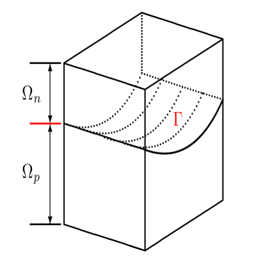
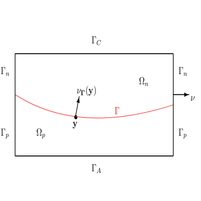
Figure 1. Left: device domain. Right: domain boundary and interface.

Inside $\Omega$ we admit the presence of an open, regular surface $\Gamma$ (called from now on the interface) that divides $\Omega$ into the two regions (connected open sets) $\Omega_{n}$ and $\Omega_{p}$ in such a way that $\Omega=\Omega_{n}\cup\Gamma\cup\Omega_{p}$. The unit normal vector oriented from $\Omega_{p}$ into $\Omega_{n}$ is denoted by $\nu_{\Gamma}$. A graphical plot of the three-dimensional (3D) domain comprising the interface is depicted in Fig. 1. The boundary of $\Omega$ is the union of two disjoint subsets, so that $\partial\Omega=\Gamma_{D}\cup\Gamma_{N}$. The unit outward normal vector on $\partial\Omega$ is denoted by $\nu$. Specifically, $\Gamma_{D}$ represents the contacts of the device, i.e. anode $\Gamma_{A}=\Gamma_{D}\cap\partial\Omega_{p}$ and cathode $\Gamma_{C}=\Gamma_{D}\cap\partial\Omega_{n}$. We assume that anode and cathode have nonzero areas and that $\Gamma_{D}$ and $\Gamma$ are strictly separated. Furthermore, $\Gamma_{N}$ is the (relatively open) part of its boundary where the device is insulated from the surrounding environment. We put $\Gamma_{n}=\Gamma_{N}\cap\partial\Omega_{n}$ and $\Gamma_{p}=\Gamma_{N}\cap\partial\Omega_{p}$. A graphical plot of a two-dimensional (2D) cross-section of the device domain comprising the interface and the boundary is depicted in Fig. 1.

The notation of function spaces in the present paper is as follows. We define $\mathcal{W}^{q}$ ($q\geq 2$) as the closure of the set

$$\left\{\left.w\right|_{\Omega}:w\in C^{\infty}\left(\mathbb{R}^{3}\right),\text{ supp}\left(w\right)\cap\Gamma_{D}=\varnothing\right\}$$

in $W^{1,q}\left(\Omega\right)$, that is, $\mathcal{W}^{q}$ is the subspace of functions belonging to $W^{1,q}\left(\Omega\right)$ which vanish on $\Gamma_{D}$ in the sense of traces

$$\mathcal{W}^{q}=\left\{w\in W^{1,q}\left(\Omega\right):\left.w\right|_{\Gamma_{D}}=0\right\}.$$

Furthermore, we define $\mathcal{W}^{-q^{\prime}}\equiv\left(\mathcal{W}^{q}\right)^{\prime}$ as the dual of $\mathcal{W}^{q}$ where $1/q+1/q^{\prime}=1$. $\mathcal{W}^{q}$ is a Banach space with respect to the usual norm in $W^{1,q}\left(\Omega\right)$. Due to meas$\left(\Gamma_{D}\right)>0$, the Poincaré inequality holds so that $\mathcal{W}^{q}$ can also be equipped with the equivalent norm

(1) $$\left\|w\right\|_{\mathcal{W}^{q}}=\left\|\nabla w\right\|_{L^{q}\left(\Omega\right)}.$$

In analogy with the definition of $\mathcal{W}^{q}$, we set

$$\mathcal{W}_{n}^{q}=\left\{w\in W^{1,q}\left(\Omega_{n}\right):\left.w\right|_{\Gamma_{C}}=0\right\},$$

$$\mathcal{W}_{p}^{q}=\left\{w\in W^{1,q}\left(\Omega_{p}\right):\left.w\right|_{\Gamma_{A}}=0\right\}$$

with norms ($i=n,p$)

(2) $$\left\|w\right\|_{\mathcal{W}_{i}^{q}}=\left\|\nabla w\right\|_{L^{q}\left(\Omega_{i}\right)}.$$

3. Model equations

In this section we illustrate the mathematical model of the OSC schematically represented in Fig. 1. For a detailed derivation of the equation system and the validation of its physical accuracy, we invite the reader to consult [11] and all references cited therein. For convenience, a list of all the variables and parameters of the cell model together with their units is contained in Tab. 1.

symbol	description	units
$e\left(t,\mathbf{x}\right)$	concentration of excitons	m-3
$n\left(t,\mathbf{x}\right)$	concentration of electrons	m-3
$p\left(t,\mathbf{x}\right)$	concentration of holes	m-3
$P\left(t,\mathbf{y}\right)$	areal concentration of polarons	m-2
$\tau_{d}$	exciton-polaron dissociation time	s
$\tau_{e}$	exciton lifetime	s
$k_{d}$	polaron dissociation rate	s-1
$k_{r}$	polaron-exciton recombination rate	s-1
$\gamma$	bimolecular recombination coefficient	m3s-1
$\eta$	polaron-exciton recombination fraction
$q$	quantum of charge	C
$D_{e}$, $D_{n}$, $D_{p}$	exciton (electron, hole) diffusion coefficient	m2s-1
$\mu_{n}$, $\mu_{p}$	electron (hole) mobility	m2V-1s-1
$Q$	exciton photogeneration rate	m-3s-1
$\mathbf{J}_{e}=-D_{e}\nabla e$	exciton flux density	m-2s-1
$\mathbf{J}_{n}=q\left(D_{n}\nabla n+\mu_{n}n\mathbf{E}\right)$	electron current density	Cm-2s-1
$\mathbf{J}_{p}=q\left(-D_{p}\nabla p+\mu_{p}p\mathbf{E}\right)$	hole current density	Cm-2s-1
$\varphi\left(t,\mathbf{x}\right)$	electric potential	V
$\mathbf{E}=-\nabla\varphi$	electric field	Vm${}^{-1}=$ NC-1
$E=\left|\mathbf{E}\right|=\left|\nabla\varphi\right|$	electric field intensity
$\widetilde{\varepsilon}$	electric permittivity	CV-1m${}^{-1}=$ C2N-1m-2
$\varepsilon=\widetilde{\varepsilon}/q$	electric permittivity per unit charge	V-1m${}^{-1}=$ C2N-1m-2
$H$	interface half- width	m

Table 1. Variables, coefficients and parameters of the solar cell model.

The equations for the description of exciton generation and dynamics inside the bulk of the device material read

(3a) $$\dfrac{\partial e}{\partial t}-\nabla\cdot\left(D_{e}\nabla e\right)=Q-\dfrac{e}{\tau_{e}} \text{in }\Omega\setminus\Gamma\qquad\text{for }t>0$$

(3b) $$\llbracket e\rrbracket=0 \text{on }\Gamma\qquad\text{for }t>0$$

(3c) $$\llbracket-D_{e}\dfrac{\partial e}{\partial\nu_{\Gamma}}\rrbracket=\eta k_{r}P-\dfrac{2H}{\tau_{d}}e \text{on }\Gamma\qquad\text{for }t>0$$

(3d) $$e=0 \text{on }\Gamma_{D}\qquad\text{for }t>0$$

(3e) $$\dfrac{\partial e}{\partial\nu}=0 \text{on }\Gamma_{N}\qquad\text{for }t>0$$

(3f) $$e\left(0,\mathbf{x}\right)=e_{0}\left(\mathbf{x}\right) \text{in }\Omega\qquad\text{for }t=0.$$

Remark 1.

The boundary condition (3d) corresponds to assuming that perfect exciton quenching occurs at the contacts (see [33]).

The equations for the description of electron generation and dynamics inside the donor phase of the solar cell material read

(4a) $$\dfrac{\partial n}{\partial t}-\nabla\cdot\left(D_{n}\nabla n-\mu_{n}n\nabla\varphi\right)=0 \text{in }\Omega_{n}\qquad\text{for }t>0$$

(4b) $$D_{n}\dfrac{\partial n}{\partial\nu_{\Gamma}}=\mu_{n}\dfrac{\partial\varphi}{\partial\nu_{\Gamma}}n\mathbf{-}k_{d}P+2H\gamma np \text{on }\Gamma\qquad\text{for }t>0$$

(4c) $$n\equiv 0 \text{in }\Omega_{p}\qquad\text{for }t>0$$

(4d) $$n=0 \text{on }\Gamma_{C}\qquad\text{for }t>0$$

(4e) $$D_{n}\dfrac{\partial n}{\partial\nu}=\mu_{n}\dfrac{\partial\varphi}{\partial\nu}n \text{on }\Gamma_{n}\qquad\text{for }t>0$$

(4f) $$n\left(0,\mathbf{x}\right)=n_{0}\left(\mathbf{x}\right) \text{in }\Omega_{n}\cup\Gamma\qquad\text{for }t=0.$$

Remark 2.

The boundary condition (4d) corresponds to assuming an infinite recombination velocity at the cathode.

The equations for the description of hole generation and dynamics inside the acceptor phase of the solar cell material read

(5a) $$\dfrac{\partial p}{\partial t}-\nabla\cdot\left(D_{p}\nabla p+\mu_{p}p\nabla\varphi\right)=0 \text{in }\Omega_{p}\qquad\text{for }t>0$$

(5b) $$D_{p}\dfrac{\partial p}{\partial\nu_{\Gamma}}=-\mu_{p}\dfrac{\partial\varphi}{\partial\nu_{\Gamma}}p\mathbf{+}k_{d}P-2H\gamma np \text{on }\Gamma\qquad\text{for }t>0$$

(5c) $$p\equiv 0 \text{in }\Omega_{n}\qquad\text{for }t>0$$

(5d) $$p=0 \text{on }\Gamma_{A}\qquad\text{for }t>0$$

(5e) $$D_{p}\dfrac{\partial p}{\partial\nu}=-\mu_{p}\dfrac{\partial\varphi}{\partial\nu}p \text{on }\Gamma_{p}\qquad\text{for }t>0$$

(5f) $$p\left(0,\mathbf{x}\right)=p_{0}\left(\mathbf{x}\right) \text{in }\Omega_{p}\cup\Gamma\qquad\text{for }t=0.$$

Remark 3.

The boundary condition (5d) corresponds to assuming an infinite recombination velocity at the anode.

The equations for the description of polaron generation and dynamics on the interface separating the two material phases of the solar cell material read

(6a) $$P\equiv 0 \text{in }\Omega_{n}\cup\Omega_{p}\qquad\text{for }t>0$$

(6b) $$\dfrac{\partial P}{\partial t}=\dfrac{2H}{\tau_{d}}e+2H\gamma np-\left(k_{d}+k_{r}\right)P \text{on }\Gamma\qquad\text{for }t>0$$

(6c) $$P\left(0,\mathbf{x}\right)=P_{0}\left(\mathbf{x}\right) \text{on }\Gamma\qquad\text{for }t=0.$$

The equations for the description of electric potential distribution inside the bulk of the device material read

(7a) $$-\nabla\cdot\left(\varepsilon\nabla\varphi\right)=-n \text{in }\Omega_{n}$$

(7b) $$-\nabla\cdot\left(\varepsilon\nabla\varphi\right)=+p \text{in }\Omega_{p}$$

(7c) $$\llbracket\varphi\rrbracket=0 \text{on }\Gamma$$

(7d) $$\llbracket\varepsilon\dfrac{\partial\varphi}{\partial\nu_{\Gamma}}\rrbracket=0 \text{on }\Gamma$$

(7e) $$\varphi=\varphi_{C}\left(\mathbf{x}\right) \text{on }\Gamma_{C}$$

(7f) $$\varphi=\varphi_{A}\left(\mathbf{x}\right) \text{on }\Gamma_{A}$$

(7g) $$\dfrac{\partial\varphi}{\partial\nu}=0 \text{on }\Gamma_{n}\cup\Gamma_{p}.$$

Remark 4.

Condition (7c) expresses the physical fact that the potential is continuous passing from the acceptor to the donor material phase of the cell. Condition (7d) means no charge density on the interface $\Gamma$.

The general assumptions satisfied by all model coefficients and parameters throughout the paper are collected in Tab. 2.

symbol	assumption	bounds
$\tau_{d}$	constant	$\tau_{d}>0$
$\tau_{e}$	constant	$\tau_{e}>0$
$k_{d}\left(\mathbf{y}\right)$	measurable	$k_{d}\left(\mathbf{\cdot}\right)\geq 0\quad$a.e. on $\Gamma$
$k_{r}$	constant	$k_{r}>0$
$\gamma\left(\mathbf{y}\right)$	$\in L^{\infty}\left(\Gamma\right)$	$\exists\underline{\gamma},\overline{\gamma}>0\qquad\underline{\gamma}\leq\gamma\left(\mathbf{\cdot}\right)\leq\overline{\gamma}\quad$a.e. on $\Gamma$
$\eta$	constant	$0\leq\eta\leq 1$
$D_{e}\left(\mathbf{x}\right)$	$\in L^{\infty}\left(\Omega\right)$	$\exists\underline{d}_{e},\overline{d}_{e}>0\qquad\underline{d}_{e}\leq D_{e}\left(\mathbf{\cdot}\right)\leq\overline{d}_{e}\quad$a.e. in $\Omega$
$D_{n}\left(\mathbf{x}\right)$	$\in L^{\infty}\left(\Omega_{n}\right)$	$\exists\underline{d}_{n},\overline{d}_{n}>0\qquad\underline{d}_{n}\leq D_{n}\left(\mathbf{\cdot}\right)\leq\overline{d}_{n}\quad$a.e. in $\Omega_{n}$
$D_{p}\left(\mathbf{x}\right)$	$\in L^{\infty}\left(\Omega_{p}\right)$	$\exists\underline{d}_{p},\overline{d}_{p}>0\qquad\underline{d}_{p}\leq D_{p}\left(\mathbf{\cdot}\right)\leq\overline{d}_{p}\quad$a.e. in $\Omega_{p}$
$\mu_{n}\left(\mathbf{x},E\right)$	$\in Car\left(\overline{\Omega_{n}}\times\mathbb{R}\right)$	$\exists\overline{\mu}_{n}>0\qquad 0\leq\mu_{n}\left(\mathbf{\cdot},E\right)\leq\overline{\mu}_{n}\quad$a.e. in $\overline{\Omega_{n}}$, $\forall E\geq 0$
$\mu_{p}\left(\mathbf{x},E\right)$	$\in Car\left(\overline{\Omega_{p}}\times\mathbb{R}\right)$	$\exists\overline{\mu}_{p}>0\qquad 0\leq\mu_{p}\left(\mathbf{\cdot},E\right)\leq\overline{\mu}_{p}\quad$a.e. in $\overline{\Omega_{p}}$, $\forall E\geq 0$
$Q\left(\mathbf{x}\right)$	$\in L^{2}\left(\Omega\right)$	$Q\left(\mathbf{\cdot}\right)\geq 0\quad$a.e. in $\Omega$
$\varepsilon\left(\mathbf{x}\right)$	$\in L^{\infty}\left(\Omega\right)$	$\exists\underline{\varepsilon},\overline{\varepsilon}>0\qquad\underline{\varepsilon}\leq\varepsilon\left(\mathbf{\cdot}\right)\leq\overline{\varepsilon}\quad$a.e. in $\Omega$
$H\left(\mathbf{y}\right)$	$\in L^{\infty}\left(\Gamma\right)$	$\exists\overline{h}>0\qquad 0\leq H\left(\mathbf{\cdot}\right)\leq\overline{h}\quad$a.e. on $\Gamma$

Table 2. Assumptions on model coefficients and parameters.

4. The auxiliary Poisson problem

The elliptic boundary value problem for the electric potential (7) can be written in more compact form as

(8a) $$-\nabla\cdot\left(\varepsilon\left(\cdot\right)\nabla\varphi\right)=g\left(n,p\right) \text{in }\Omega\diagdown\Gamma$$

(8b) $$\llbracket\varphi\rrbracket=\llbracket\varepsilon\left(\cdot\right)\dfrac{\partial\varphi}{\partial\nu_{\Gamma}}\rrbracket=0 \text{on }\Gamma$$

(8c) $$\varphi=\varphi_{D} \text{on }\Gamma_{D}$$

(8d) $$\dfrac{\partial\varphi}{\partial\nu}=0 \text{on }\Gamma_{N}$$

where

(9) $$g\left(n,p\right):=\left\{\begin{array}[]{ll}-n&\qquad\text{in }\Omega_{n}\\ +p&\qquad\text{in }\Omega_{p}\end{array}\right.$$

and

(10) $$\varphi_{D}:=\left\{\begin{array}[]{ll}\varphi_{C}&\qquad\text{on }\Gamma_{C}\\ \varphi_{A}&\qquad\text{on }\Gamma_{A}.\end{array}\right.$$

We assume that the electric permittivity $\varepsilon$ is as specified in Tab. 2 and that there exists $\widetilde{\varphi}\in H^{1}\left(\Omega\right)$ whose trace on $\partial\Omega$ is equal to $\varphi_{D}$ on $\Gamma_{D}$. Next, for the moment let $g\in L^{2}\left(\Omega\right)$ be a given function and consider the following linear elliptic transmission problem with mixed boundary conditions (from now on referred to as auxiliary Poisson problem):

(11a) $$-\nabla\cdot\left(\varepsilon\left(\cdot\right)\nabla\varphi\right)=g\left(\cdot\right) \text{in }\Omega\diagdown\Gamma$$

(11b) $$\llbracket\varphi\rrbracket=\llbracket\varepsilon\left(\cdot\right)\dfrac{\partial\varphi}{\partial\nu_{\Gamma}}\rrbracket=0 \text{on }\Gamma$$

(11c) $$\varphi=\varphi_{D} \text{on }\Gamma_{D}$$

(11d) $$\dfrac{\partial\varphi}{\partial\nu}=0 \text{on }\Gamma_{N}.$$

Let $u=\varphi-\widetilde{\varphi}$. Then the auxiliary problem (11) is equivalent to

(12a) $$-\nabla\cdot\left(\varepsilon\left(\cdot\right)\nabla u\right)=g\left(\cdot\right)+\nabla\cdot\left(\varepsilon\left(\cdot\right)\nabla\widetilde{\varphi}\right) \qquad\text{in }\Omega$$

(12b) $$u=0 \text{on }\Gamma_{D}$$

(12c) $$\dfrac{\partial u}{\partial\nu}=-\dfrac{\partial\widetilde{\varphi}}{\partial\nu} \text{on }\Gamma_{N}.$$

Definition 5.

$u\in\mathcal{W}^{2}$ is called a variational solution to the auxiliary Poisson problem (12) if

(13) $$a\left(u,v\right)=L\left(v\right)\qquad\forall v\in\mathcal{W}^{2}$$

where

$$a\left(u,v\right)=\int_{\Omega}\varepsilon\left(\cdot\right)\nabla u\cdot\nabla vdx \qquad u,v\in\mathcal{W}^{2},$$

$$L\left(v\right)=\int_{\Omega}g\left(\cdot\right)vdx-\int_{\Omega}\varepsilon\left(\cdot\right)\nabla\widetilde{\varphi}\cdot\nabla vdx \qquad v\in\mathcal{W}^{2}.$$

It is easily verified that $a$ and $L$ satisfy the hypotheses of the Lax-Milgram Lemma. As a consequence, the following result can be proved.

Lemma 6 (auxiliary Poisson problem, #1).

Assume $\varepsilon\left(\cdot\right)$ as specified in Tab. 2, $g\in L^{2}\left(\Omega\right)$ and that there exists $\widetilde{\varphi}\in H^{1}\left(\Omega\right)$ whose trace on $\partial\Omega$ is equal to $\varphi_{D}$ on $\Gamma_{D}$. Then there is a unique weak solution $\varphi$ to problem (11) in the function class $\varphi-\widetilde{\varphi}=u\in\mathcal{W}^{2}$ and the following estimate holds

(14) $$\left\|u\right\|_{\mathcal{W}^{2}}\leq\frac{c}{\underline{\varepsilon}}\left\|g\right\|_{L^{2}\left(\Omega\right)}+\frac{\overline{\varepsilon}}{\underline{\varepsilon}}\left\|\nabla\widetilde{\varphi}\right\|_{L^{2}\left(\Omega\right)}$$

for some $c=c\left(\Omega\right)>0$.

In order to prove the existence of a weak solution to the DD system we need a stronger solution to the auxiliary Poisson problem. To this end, consider the elliptic operator $-\nabla\cdot\varepsilon\nabla:\mathcal{W}^{2}\rightarrow\mathcal{W}^{-2}$ defined by

$$\left\langle-\nabla\cdot\left(\varepsilon\left(\cdot\right)\nabla u\right),v\right\rangle_{\mathcal{W}^{-2}}:=a\left(u,v\right),\qquad u,v\in\mathcal{W}^{2}$$

and use the same notation $-\nabla\cdot\varepsilon\nabla$ for the restriction of this operator to the spaces $\mathcal{W}^{q}$ ($q>2$). Then, it is clear that it is a continuous operator from $\mathcal{W}^{q}$ into $\mathcal{W}^{-q}\equiv\left(\mathcal{W}^{q^{\prime}}\right)^{\prime}$. However, it would be desirable that $-\nabla\cdot\varepsilon\nabla:\mathcal{W}^{q}\rightarrow\mathcal{W}^{-q}$ provides a topological isomorphism for some $q>2$, i.e. a one-to-one continuous mapping of $\mathcal{W}^{q}$ onto $\mathcal{W}^{-q}$ for which the inverse mapping is also continuous. Since it is well known that this isomorphism property is actually an assumption on $\Omega$, $\Gamma_{D}$ and $\Gamma_{N}$ (see [25, 5] and [16, 17, 6, 18, 19, 15]), we shall call $q-$admissible any triple $\left\{\Omega,\Gamma_{D},\Gamma_{N}\right\}$ such that the stated property holds.

Lemma 7 (auxiliary Poisson problem, #2).

Assume that $\left\{\Omega,\Gamma_{D},\Gamma_{N}\right\}$ is a $q-$admissible triple for some $q>2$, $\varepsilon\left(\cdot\right)$ as specified in Tab. 2, $g\in L^{q}\left(\Omega\right)$ and that there exists $\widetilde{\varphi}\in W^{1.q}\left(\Omega\right)$ whose trace on $\partial\Omega$ is equal to $\varphi_{D}$ on $\Gamma_{D}$. Then there is a unique solution $\varphi$ to problem (11) in the function class $\varphi-\widetilde{\varphi}=u\in\mathcal{W}^{q}$ and the following estimate holds

(15) $$\left\|u\right\|_{\mathcal{W}^{q}}\leq c\left\{\left\|g\right\|_{L^{q}\left(\Omega\right)}+\left\|\nabla\widetilde{\varphi}\right\|_{L^{q}\left(\Omega\right)}\right\}$$

for some $c=c\left(q,\Omega,\varepsilon\right)>0$.

Proof.

Set $\psi=g\left(\cdot\right)+\nabla\cdot\left(\varepsilon\left(\cdot\right)\nabla\widetilde{\varphi}\right)$. Then $\psi\in\left(W^{1,q^{\prime}}\left(\Omega\right)\right)^{\prime}$, the dual of $W^{1,q^{\prime}}\left(\Omega\right)$ (see [35], Th. 4.3.2, p.186). But the inclusion $\mathcal{W}^{q^{\prime}}\subset W^{1,q^{\prime}}\left(\Omega\right)$ implies $\left(W^{1,q^{\prime}}\left(\Omega\right)\right)^{\prime}\subset\left(\mathcal{W}^{q^{\prime}}\right)^{\prime}\equiv\mathcal{W}^{-q}$ so that the right-hand side of (12a) is an element of $\mathcal{W}^{-q}$. Then by $q-$admissibility there is a unique solution $u\in\mathcal{W}^{q}$ to problem (12) and

$$\left\|u\right\|_{\mathcal{W}^{q}}\leq c\left(q,\Omega,\varepsilon\right)\left\|\psi\right\|_{\mathcal{W}^{-q}}.$$

Now, $q>2$ implies $q^{\prime}<2$ so that $\mathcal{W}^{q}\subset\mathcal{W}^{2}\subset\mathcal{W}^{q^{\prime}}$. Then, for $v\in\mathcal{W}^{2}$, we have by Hölder’s inequality

$$\left|\left\langle\psi,v\right\rangle_{\mathcal{W}^{-q}}\right|=\left|\int_{\Omega}\left(gv-\varepsilon\nabla\widetilde{\varphi}\cdot\nabla v\right)dx\right|$$

$$\leq\left\|g\right\|_{L^{q}\left(\Omega\right)}\left\|v\right\|_{L^{q\prime}\left(\Omega\right)}+\overline{\varepsilon}\left\|\nabla\widetilde{\varphi}\right\|_{L^{q}\left(\Omega\right)}\left\|\nabla v\right\|_{L^{q\prime}\left(\Omega\right)}$$

$$\leq c\left(q,\Omega\right)\left(\left\|g\right\|_{L^{q}\left(\Omega\right)}+\overline{\varepsilon}\left\|\nabla\widetilde{\varphi}\right\|_{L^{q}\left(\Omega\right)}\right)\left\|v\right\|_{\mathcal{W}^{q^{\prime}}}.$$

By density the above estimate holds for all $v\in\mathcal{W}^{q^{\prime}}$ hence

$$\left\|\psi\right\|_{\mathcal{W}^{-q}}\leq c\left(q,\Omega\right)\left(\left\|g\right\|_{L^{q}\left(\Omega\right)}+\overline{\varepsilon}\left\|\nabla\widetilde{\varphi}\right\|_{L^{q}\left(\Omega\right)}\right)$$

and (15) follows. ∎

Remark 8.

Lemma 7 guarantees that $\varphi\in W^{1,q}\left(\Omega\right)$, hence (the restrictions) $\nabla\varphi\in L^{q}\left(\Omega_{n}\right)$ and $\nabla\varphi\in L^{q}\left(\Omega_{p}\right)$. Moreover, using (1) and (15), we get

$$\left\|\nabla\varphi\right\|_{L^{q}\left(\Omega_{n}\right)}\leq\left\|\nabla u\right\|_{L^{q}\left(\Omega_{n}\right)}+\left\|\nabla\widetilde{\varphi}\right\|_{L^{q}\left(\Omega_{n}\right)}\leq\left\|u\right\|_{\mathcal{W}^{q}}+\left\|\nabla\widetilde{\varphi}\right\|_{L^{q}\left(\Omega_{n}\right)}$$

$$\leq c\left(q,\Omega,\varepsilon\right)\left(\left\|g\right\|_{L^{q}\left(\Omega\right)}+\left\|\nabla\widetilde{\varphi}\right\|_{L^{q}\left(\Omega\right)}\right)+\left\|\nabla\widetilde{\varphi}\right\|_{L^{q}\left(\Omega_{n}\right)}$$

(16) $$\leq\left\{c\left(q,\Omega,\varepsilon\right)+1\right\}\left(\left\|g\right\|_{L^{q}\left(\Omega\right)}+\left\|\nabla\widetilde{\varphi}\right\|_{L^{q}\left(\Omega\right)}\right)$$

and a similar estimate holds true for $\left\|\nabla\varphi\right\|_{L^{q}\left(\Omega_{p}\right)}$.

5. The multiscale model in the stationary case

In this section we examine the multiscale model of Sect. 3 in stationary conditions. This corresponds to setting to zero all partial derivatives with respect to the time variable $t$ and to assuming that all coefficients and unknowns depend on the sole spatial variable $\mathbf{x}$.

5.1. Polarons

Eq. (6b) has the explicit stationary solution for $\mathbf{y}\in\Gamma$

(17) $$P\left(\mathbf{y}\right)=\dfrac{2H\left(\mathbf{y}\right)}{\left(k_{d}\left(\mathbf{y}\right)+k_{r}\right)\tau_{d}}\,e\left(\mathbf{y}\right)+\dfrac{2H\left(\mathbf{y}\right)\gamma\left(\mathbf{y}\right)}{k_{d}\left(\mathbf{y}\right)+k_{r}}\,n\left(\mathbf{y}\right)p\left(\mathbf{y}\right)$$

and this expression has to be inserted into the condition on $\Gamma$ of the stationary problems for excitons, electrons and holes. This is done in the next sections.

5.2. The auxiliary exciton problem

Upon inserting (17) into (3c) the stationary problem for the excitons reads

(18a) $$-\nabla\cdot\left(D_{e}\left(\cdot\right)\nabla e\right)+\tau_{e}^{-1}e=Q\left(\cdot\right) \qquad\text{in }\Omega\setminus\Gamma$$

(18b) $$\llbracket e\rrbracket=0 \qquad\text{on }\Gamma$$

(18c) $$\llbracket D_{e}\left(\cdot\right)\dfrac{\partial e}{\partial\nu_{\Gamma}}\rrbracket=\alpha\left(\cdot\right)e-\beta\left(\cdot\right)f\left(n,p\right) \text{on }\Gamma$$

(18d) $$e=0 \text{on }\Gamma_{D}$$

(18e) $$\dfrac{\partial e}{\partial\nu}=0 \text{on }\Gamma_{N}$$

where we have set (for all $\mathbf{y}\in\Gamma$)

(19) $$\alpha\left(\mathbf{y}\right):=\dfrac{2H\left(\mathbf{y}\right)}{\tau_{d}}\times\dfrac{k_{d}\left(\mathbf{y}\right)+\left(1-\eta\right)k_{r}}{k_{d}\left(\mathbf{y}\right)+k_{r}}=\dfrac{2H\left(\mathbf{y}\right)}{\tau_{d}}-\dfrac{\beta\left(\mathbf{y}\right)}{\gamma\left(\mathbf{y}\right)\tau_{d}}$$

(20) $$\beta\left(\mathbf{y}\right):=\dfrac{2\eta k_{r}\gamma\left(\mathbf{y}\right)H\left(\mathbf{y}\right)}{k_{d}\left(\mathbf{y}\right)+k_{r}}$$

(21) $$f\left(n,p\right):=np.$$

Taking into account the bounds stated in Tab. 2 the functions $\alpha$ and $\beta$ satisfy the following constraints:

$$0\leq\left(1-\eta\right)\dfrac{2H\left(\cdot\right)}{\tau_{d}}\leq\alpha\left(\cdot\right)\leq\dfrac{2H\left(\cdot\right)}{\tau_{d}}\leq\dfrac{2\overline{h}}{\tau_{d}}=:\overline{\alpha}$$

$$0\leq\beta\left(\cdot\right)\leq 2\eta H\left(\cdot\right)\gamma\left(\cdot\right)\leq 2\eta\overline{h}\overline{\gamma}=:\overline{\beta}$$

For the moment let $f$ be a given function. Then the transmission problem (18) is referred to as the auxiliary exciton problem:

(22a) $$-\nabla\cdot\left(D_{e}\left(\cdot\right)\nabla e\right)+\tau_{e}^{-1}e=Q\left(\cdot\right) \qquad\text{in }\Omega\setminus\Gamma$$

(22b) $$\llbracket e\rrbracket=0 \qquad\text{on }\Gamma$$

(22c) $$\llbracket D_{e}\left(\cdot\right)\dfrac{\partial e}{\partial\nu_{\Gamma}}\rrbracket=\alpha\left(\cdot\right)e-\beta\left(\cdot\right)f\left(\cdot\right) \text{on }\Gamma$$

(22d) $$e=0 \text{on }\Gamma_{D}$$

(22e) $$\dfrac{\partial e}{\partial\nu}=0 \text{on }\Gamma_{N}.$$

Definition 9.

$e\in\mathcal{W}^{2}$ is called a variational solution to the auxiliary exciton problem (22) if

(23) $$b\left(e,v\right)=\ell\left(v\right)\qquad\forall v\in\mathcal{W}^{2}$$

where

$$b\left(u,v\right)=\int_{\Omega}D_{e}\left(\cdot\right)\nabla u\cdot\nabla vdx+\tau_{e}^{-1}\int_{\Omega}uvdx+\int_{\Gamma}\alpha\left(\cdot\right)uvd\sigma$$

$$\ell\left(v\right)=\int_{\Omega}Q\left(\cdot\right)vdx+\int_{\Gamma}\beta\left(\cdot\right)f\left(\cdot\right)vd\sigma.$$

Lemma 10 (Auxiliary exciton problem).

Let $D_{e}$, $\tau_{e}$, $Q$ be as specified in Tab. 2; $f\in L^{2}\left(\Gamma\right)$; $\alpha,\beta\in L^{\infty}\left(\Gamma\right)$ and $0\leq\alpha\leq\overline{\alpha}$, $0\leq\beta\leq\overline{\beta}$ a.e. on $\Gamma$ for some constants $\overline{\alpha},\overline{\beta}>0$. Then there is a unique variational solution $e$ to (22). If in addition $f\geq 0$ a.e. on $\Gamma$, then the solution $e\geq 0$ a.e. in $\Omega$.

Proof.

(Existence and uniqueness) By the Sobolev Imbedding Theorem on submanifolds we have $H^{1}\left(\Omega\right)\hookrightarrow L^{q}\left(\Gamma\right)$ for all $q\in\left[2,4\right]$. Thus, there exists a constant $c=c\left(q,\Omega,\Gamma\right)$ such that

$$\left\|v\right\|_{L^{q}\left(\Gamma\right)}\leq c\left\|v\right\|_{H^{1}\left(\Omega\right)}\qquad\qquad\forall v\in H^{1}\left(\Omega\right)$$

hence we obtain, in particular,

(24) $$\left\|v\right\|_{L^{q}\left(\Gamma\right)}\leq c\left\|v\right\|_{\mathcal{W}^{2}}\qquad\forall v\in\mathcal{W}^{2}.$$

Then, using (24) with $q=2$, we have

$$\left|b\left(u,v\right)\right| \leq \int_{\Omega}\left|D_{e}\nabla u\cdot\nabla v\right|dx+\tau_{e}^{-1}\int_{\Omega}\left|uv\right|dx+\int_{\Gamma}\left|\alpha uv\right|d\sigma$$

$$\leq \overline{d}_{e}\left\|\nabla u\right\|_{L^{2}\left(\Omega\right)}\left\|\nabla v\right\|_{L^{2}\left(\Omega\right)}+\tau_{e}^{-1}\left\|u\right\|_{L^{2}\left(\Omega\right)}\left\|v\right\|_{L^{2}\left(\Omega\right)}+\overline{\alpha}\left\|u\right\|_{L^{2}\left(\Gamma\right)}\left\|v\right\|_{L^{2}\left(\Gamma\right)}$$

$$\leq \left(\overline{d}_{e}+\tau_{e}^{-1}c\left(\Omega\right)+c\left(\Omega,\Gamma\right)\overline{\alpha}\right)\left\|u\right\|_{\mathcal{W}^{2}}\left\|v\right\|_{\mathcal{W}^{2}}\qquad\qquad\qquad\forall u,v\in\mathcal{W}^{2}.$$

This shows that $b\left(u,v\right)$ is continuous on $\mathcal{W}^{2}\times\mathcal{W}^{2}$. Furthermore, $b\left(u,v\right)$ is coercive on $\mathcal{W}^{2}\times\mathcal{W}^{2}$ because

$$b\left(v,v\right)\geq\underline{d}_{e}\int_{\Omega}\left|\nabla v\right|^{2}dx=\underline{d}_{e}\left\|v\right\|_{\mathcal{W}^{2}}^{2} \qquad\forall v\in\mathcal{W}^{2}$$

(recall that $\tau_{e}>0$ and $\alpha\geq 0$). Finally, $\ell\left(v\right)$ is continuous on $\mathcal{W}^{2}$ because

$$\left|\ell\left(v\right)\right| \leq \left\|Q\right\|_{L^{2}\left(\Omega\right)}\left\|v\right\|_{L^{2}\left(\Omega\right)}+\overline{\beta}\left\|f\right\|_{L^{2}\left(\Gamma\right)}\left\|v\right\|_{L^{2}\left(\Gamma\right)}$$

$$\leq \left(c\left(\Omega\right)\left\|Q\right\|_{L^{2}\left(\Omega\right)}+c\left(\Omega,\Gamma\right)\overline{\beta}\left\|f\right\|_{L^{2}\left(\Gamma\right)}\right)\left\|v\right\|_{\mathcal{W}^{2}}\qquad\qquad\qquad\forall v\in\mathcal{W}^{2}.$$

Then the assertion follows by the Lax-Milgram Lemma.

(Positivity) Define $e^{+}=\max\left\{e,0\right\}$ and $e^{-}=\max\left\{-e,0\right\}$. Then $e^{+},e^{-}\geq 0$ and $e=e^{+}-e^{-}$. Since $e^{-}\in\mathcal{W}^{2}$, we can choose $v=e^{-}$ in (23) to get

$$b\left(e^{+}-e^{-},e^{-}\right)=\ell\left(e^{-}\right).$$

But $\ell\left(e^{-}\right)\geq 0$ so that

$$0\leq b\left(e^{-},e^{-}\right)\leq b\left(e^{+},e^{-}\right).$$

Let $\Omega_{+}=\left\{e\geq 0\right\}$ and $\Omega_{-}=\left\{e\leq 0\right\}$: then $\left.e^{+}\right|_{\Omega_{-}}=0$, $\left.e^{-}\right|_{\Omega_{+}}=0$, hence $e^{+}e^{-}=0$ in $\Omega=\Omega_{+}\cup\Omega_{-}$. As a consequence we have also $e^{+}e^{-}=0$ in $\Gamma$ and $\nabla e^{+}\cdot\nabla e^{-}=0$ in $\Omega$, so that $b\left(e^{+},e^{-}\right)=0$. In conclusion $b\left(e^{-},e^{-}\right)=0$, from which it follows $e^{-}=0$, i.e. $e=e^{+}\geq 0$ in $\Omega$. ∎

Remark 11.

From (23) where $v=e$ is chosen, we see that

$$\underline{d}_{e}\left\|e\right\|_{\mathcal{W}^{2}}^{2}\leq b\left(e,e\right)=\ell\left(e\right)\leq\left(c\left(\Omega\right)\left\|Q\right\|_{L^{2}\left(\Omega\right)}+c\left(\Omega,\Gamma\right)\overline{\beta}\left\|f\right\|_{L^{2}\left(\Gamma\right)}\right)\left\|e\right\|_{\mathcal{W}^{2}}$$

hence the variational solution $e$ of (22) satisfies the estimate

(25) $$\left\|e\right\|_{\mathcal{W}^{2}}\leq\frac{c\left(\Omega\right)}{\underline{d}_{e}}\left\|Q\right\|_{L^{2}\left(\Omega\right)}+\frac{c\left(\Omega,\Gamma\right)}{\underline{d}_{e}}\overline{\beta}\left\|f\right\|_{L^{2}\left(\Gamma\right)}$$

for some constants $c\left(\Omega\right)>0$, $c\left(\Omega,\Gamma\right)>0$.

5.3. The auxiliary electron problem

Upon inserting (17) into (4b) the stationary problem for the electrons reads

(26a) $$-\nabla\cdot\left(D_{n}\left(\cdot\right)\nabla n-\mu_{n}\left(\cdot,\left|\nabla\varphi\right|\right)n\nabla\varphi\right)=0 \qquad\text{in }\Omega_{n}$$

(26b) $$D_{n}\left(\cdot\right)\dfrac{\partial n}{\partial\nu_{\Gamma}}=\mu_{n}\left(\cdot,\left|\nabla\varphi\right|\right)\dfrac{\partial\varphi}{\partial\nu_{\Gamma}}n+h\left(\cdot,p\right)n\mathbf{-}h_{e}\left(\cdot,e\right) \qquad\text{on }\Gamma$$

(26c) $$n=0 \qquad\text{on }\Gamma_{C}$$

(26d) $$D_{n}\left(\cdot\right)\dfrac{\partial n}{\partial\nu}=\mu_{n}\left(\cdot,\left|\nabla\varphi\right|\right)\dfrac{\partial\varphi}{\partial\nu}n \qquad\text{on }\Gamma_{n}$$

where ($\mathbf{y}\in\Gamma$)

(27) $$\omega\left(\mathbf{y}\right):=\frac{k_{d}\left(\mathbf{y}\right)}{k_{d}\left(\mathbf{y}\right)+k_{r}}\dfrac{2H\left(\mathbf{y}\right)}{\tau_{d}}$$

(28) $$h\left(\mathbf{y},p\right):=\frac{\beta\left(\mathbf{y}\right)}{\eta}p$$

(29) $$h_{e}\left(\mathbf{y},e\right):=\omega\left(\mathbf{y}\right)e$$

and where $\beta$ is defined in (20). Note that we have

(30) $$0\leq\omega\left(\cdot\right)\leq\frac{2H\left(\cdot\right)}{\tau_{d}}\leq\dfrac{2\overline{h}}{\tau_{d}}=\overline{\alpha}.$$

Now assume that the function $\varphi$ in (26) is given by $\varphi=u+\widetilde{\varphi}$ where $u$ is the solution of the auxiliary Poisson problem (12). In addition, suppose that $\mu_{n}$, $h$ and $h_{e}$ are given and known (with $\mu_{n}$ satisfying the bounds of Tab. 2). Then the transmission problem (26) is referred to as the auxiliary electron problem:

(31a) $$-\nabla\cdot\left(D_{n}\left(\cdot\right)\nabla n-\mu_{n}\left(\cdot\right)n\nabla\varphi\right)=0 \qquad\text{in }\Omega_{n}$$

(31b) $$D_{n}\left(\cdot\right)\dfrac{\partial n}{\partial\nu_{\Gamma}}=\mu_{n}\left(\cdot\right)\dfrac{\partial\varphi}{\partial\nu_{\Gamma}}n+h\left(\cdot\right)n\mathbf{-}h_{e}\left(\cdot\right) \qquad\text{on }\Gamma$$

(31c) $$n=0 \qquad\text{on }\Gamma_{C}$$

(31d) $$D_{n}\left(\cdot\right)\dfrac{\partial n}{\partial\nu}=\mu_{n}\left(\cdot\right)\dfrac{\partial\varphi}{\partial\nu}n \qquad\text{on }\Gamma_{n}.$$

Definition 12.

$n\in\mathcal{W}_{n}^{2}$ is called a variational solution to the auxiliary electron problem (31) if

(32) $$a_{n}\left(n,v\right)=L_{n}\left(v\right)\qquad\forall v\in\mathcal{W}_{n}^{2}$$

where

$$a_{n}\left(n,v\right)=\int_{\Omega_{n}}D_{n}\left(\cdot\right)\nabla n\cdot\nabla vdx-\int_{\Omega_{n}}\mu_{n}\left(\cdot\right)n\left(\nabla v\cdot\nabla\varphi\right)dx+\int_{\Gamma}h\left(\cdot\right)nvd\sigma$$

$$L_{n}\left(v\right)=\int_{\Gamma}h_{e}\left(\cdot\right)vd\sigma.$$

Lemma 13 (Auxiliary electron problem).

Assume that $\left\{\Omega,\Gamma_{D},\Gamma_{N}\right\}$ is a $q-$admissible triple for some $q\geq 3$; let $\varphi$ be given by Lemma 7; $D_{n}$, $\mu_{n}\in L^{\infty}\left(\Omega_{n}\right)$ and satisfying the bounds of Tab. 2; $h,h_{e}\in L^{2}\left(\Gamma\right)$; $h\geq 0$ a.e. on $\Gamma$. Then there is a constant $\delta>0$ such that if $\left\|\nabla\varphi\right\|_{L^{q}\left(\Omega_{n}\right)}<\delta$ then problem (31) has a unique variational solution $n$. If in addition $h_{e}\geq 0$ a.e. on $\Gamma$, then the solution $n\geq 0$ a.e. in $\Omega_{n}$.

Proof.

(Existence and uniqueness) Let us show that $a_{n}\left(u,v\right)$ is continuous on $\mathcal{W}_{n}^{2}\times\mathcal{W}_{n}^{2}$. We have

$$\left|a_{n}\left(u,v\right)\right|\leq\overline{d}_{n}\left\|\nabla u\right\|_{L^{2}\left(\Omega_{n}\right)}\left\|\nabla v\right\|_{L^{2}\left(\Omega_{n}\right)}$$

(33) $$+\overline{\mu}_{n}\int_{\Omega_{n}}\left|u\right|\,\left|\nabla v\right|\,\left|\nabla\varphi\right|\,dx+\int_{\Gamma}h\left|uv\right|d\sigma.$$

By virtue of the Hölder’s inequality for three functions the following estimate holds

(34) $$\int_{\Omega_{n}}\left|u\right|\,\left|\nabla v\right|\,\left|\nabla\varphi\right|\,dx\leq\left\|u\right\|_{L^{r}\left(\Omega_{n}\right)}\left\|\nabla v\right\|_{L^{2}\left(\Omega_{n}\right)}\left\|\nabla\varphi\right\|_{L^{q}\left(\Omega_{n}\right)}$$

where $1/r+1/q=1/2$. The continuity of the embedding $H^{1}\left(\Omega_{n}\right)\rightarrow L^{r}\left(\Omega_{n}\right)$ ($2\leq r\leq 6$) yields

(35) $$\left\|u\right\|_{L^{r}\left(\Omega_{n}\right)}\leq c\left(q,\Omega_{n}\right)\left\|u\right\|_{H^{1}\left(\Omega_{n}\right)}\leq c\left(q,\Omega_{n}\right)\left\|u\right\|_{\mathcal{W}_{n}^{2}}$$

and $2\leq r\leq 6$ implies $q\geq 3$. Therefore

(36) $$\int_{\Omega_{n}}\left|u\right|\,\left|\nabla v\right|\,\left|\nabla\varphi\right|\,dx\leq c\left(q,\Omega_{n}\right)\left\|\nabla\varphi\right\|_{L^{q}\left(\Omega_{n}\right)}\left\|u\right\|_{\mathcal{W}_{n}^{2}}\left\|v\right\|_{\mathcal{W}_{n}^{2}}.$$

In addition, using the generalized Hölder’s inequality and the continuity of trace and embedding $H^{1}\left(\Omega_{n}\right)\longrightarrow H^{1/2}\left(\partial\Omega_{n}\right)\longrightarrow L^{4}\left(\partial\Omega_{n}\right)$, gives

(37) $$\int_{\Gamma}h\left|uv\right|d\sigma \leq \left\|h\right\|_{L^{2}\left(\Gamma\right)}\left\|uv\right\|_{L^{2}\left(\Gamma\right)}\leq\left\|h\right\|_{L^{2}\left(\Gamma\right)}\left\|u\right\|_{L^{4}\left(\Gamma\right)}\left\|v\right\|_{L^{4}\left(\Gamma\right)}$$

$$\leq \left\|h\right\|_{L^{2}\left(\Gamma\right)}\left\|u\right\|_{L^{4}\left(\partial\Omega_{n}\right)}\left\|v\right\|_{L^{4}\left(\partial\Omega_{n}\right)}$$

$$\leq c\left(\Omega_{n}\right)\left\|h\right\|_{L^{2}\left(\Gamma\right)}\left\|u\right\|_{H^{1}\left(\Omega_{n}\right)}\left\|v\right\|_{H^{1}\left(\Omega_{n}\right)}$$

$$\leq c\left(\Omega_{n}\right)\left\|h\right\|_{L^{2}\left(\Gamma\right)}\left\|u\right\|_{\mathcal{W}_{n}^{2}}\left\|v\right\|_{\mathcal{W}_{n}^{2}}.$$

Inserting (36) and (37) into (5.3) yields

$$\left|a_{n}\left(u,v\right)\right|\leq\left\{\overline{d}_{n}+c\left(q,\Omega_{n}\right)\overline{\mu}_{n}\left\|\nabla\varphi\right\|_{L^{q}\left(\Omega_{n}\right)}+c\left(\Omega_{n}\right)\left\|h\right\|_{L^{2}\left(\Gamma\right)}\right\}\left\|u\right\|_{\mathcal{W}_{n}^{2}}\left\|v\right\|_{\mathcal{W}_{n}^{2}}$$

which proves the continuity of $a_{n}\left(u,v\right)$. Concerning the coercivity of $a_{n}\left(u,v\right)$, we have for $v\in\mathcal{W}_{n}^{2}$ (recall that $h\geq 0$)

$$a_{n}\left(v,v\right) = \int_{\Omega_{n}}D_{n}\left|\nabla v\right|^{2}dx-\int_{\Omega_{n}}\mu_{n}\left(\nabla\varphi\cdot\nabla v\right)vdx+\int_{\Gamma}hv^{2}d\sigma$$

$$\geq \underline{d}_{n}\int_{\Omega_{n}}\left|\nabla v\right|^{2}dx-\int_{\Omega_{n}}\mu_{n}\left(\nabla\varphi\cdot\nabla v\right)vdx$$

$$\geq \underline{d}_{n}\left\|\nabla v\right\|_{L^{2}\left(\Omega_{n}\right)}^{2}-\overline{\mu}_{n}\int_{\Omega_{n}}\left|\nabla\varphi\right|\,\left|\nabla v\right|\,\left|v\right|\,dx$$

by (36)

$$\geq \underline{d}_{n}\left\|v\right\|_{\mathcal{W}_{n}^{2}}^{2}-c\left(q,\Omega_{n}\right)\overline{\mu}_{n}\left\|\nabla\varphi\right\|_{L^{q}\left(\Omega_{n}\right)}\left\|v\right\|_{\mathcal{W}_{n}^{2}}^{2}$$

hence

$$a_{n}\left(v,v\right)\geq\Lambda_{n}\left\|v\right\|_{\mathcal{W}_{n}^{2}}^{2}\qquad\qquad\qquad\forall v\in\mathcal{W}_{n}^{2}$$

where

(38) $$\Lambda_{n}:=\underline{d}_{n}-c\left(q,\Omega_{n}\right)\overline{\mu}_{n}\left\|\nabla\varphi\right\|_{L^{q}\left(\Omega_{n}\right)}.$$

Using again the continuity of trace and embedding allows us to prove that $L_{n}\left(v\right)$ is continuous on $\mathcal{W}_{n}^{2}$:

$$\left|L_{n}\left(v\right)\right| \leq \left\|h_{e}\right\|_{L^{2}\left(\Gamma\right)}\left\|v\right\|_{L^{2}\left(\Gamma\right)}\leq\left\|h_{e}\right\|_{L^{2}\left(\Gamma\right)}\left\|v\right\|_{L^{2}\left(\partial\Omega_{n}\right)}$$

$$\leq c\left(\Omega_{n}\right)\left\|h_{e}\right\|_{L^{2}\left(\Gamma\right)}\left\|v\right\|_{\mathcal{W}_{n}^{2}}\qquad\qquad\qquad\forall v\in\mathcal{W}_{n}^{2}.$$

Then we conclude that the existence of a unique solution follows by the Lax-Milgram Lemma provided that $\Lambda_{n}>0$, i.e if

(39) $$\left\|\nabla\varphi\right\|_{L^{q}\left(\Omega_{n}\right)}<\delta:=\frac{\underline{d}_{n}}{\overline{\mu}_{n}}c\left(q,\Omega_{n}\right).$$

(Positivity) Define $n^{+}=\max\left\{n,0\right\}$ and $n^{-}=\max\left\{-n,0\right\}$. Then $n^{+},n^{-}\geq 0$ and $n=n^{+}-n^{-}$. Since $n^{-}\in\mathcal{W}_{n}^{2}$, we can choose $v=n^{-}$ in (32) to get

$$a_{n}\left(n^{+}-n^{-},n^{-}\right)=L_{n}\left(n^{-}\right).$$

But $L_{n}\left(n^{-}\right)\geq 0$ so that

$$a_{n}\left(n^{-},n^{-}\right)\leq a_{n}\left(n^{+},n^{-}\right).$$

Let $\Omega_{n}^{+}=\left\{n\geq 0\right\}$ and $\Omega_{n}^{-}=\left\{n\leq 0\right\}$: then $\Omega_{n}=\Omega_{n}^{+}\cup\Omega_{n}^{-}$ and $\left.n^{+}\right|_{\Omega_{n}^{-}}=\left.n^{-}\right|_{\Omega_{n}^{+}}=0$, hence $a_{n}\left(n^{+},n^{-}\right)=0$. In conclusion

$$0\leq\Lambda_{n}\left\|\nabla n^{-}\right\|_{L^{2}\left(\Omega_{n}\right)}^{2}\leq a_{n}\left(n^{-},n^{-}\right)\leq 0$$

from which it follows $\nabla n^{-}=0$ in $\Omega_{n}$. Then $n^{-}=0$ in $\Omega_{n}$ i.e. $n=n^{+}\geq 0$ in $\Omega_{n}$. ∎

Remark 14.

From (32) where $v=n$ is chosen, we see that

$$\Lambda_{n}\left\|n\right\|_{\mathcal{W}_{n}^{2}}^{2}\leq a_{n}\left(n,n\right)=L_{n}\left(n\right)\leq c\left(\Omega_{n}\right)\left\|h_{e}\right\|_{L^{2}\left(\Gamma\right)}\left\|n\right\|_{\mathcal{W}_{n}^{2}}$$

hence the variational solution $n$ of (31) satisfies the estimate

(40) $$\left\|n\right\|_{\mathcal{W}_{n}^{2}}\leq\frac{c\left(\Omega_{n}\right)}{\Lambda_{n}}\left\|h_{e}\right\|_{L^{2}\left(\Gamma\right)}$$

for some $c=c\left(\Omega_{n}\right)>0$.

5.4. The auxiliary hole problem

Upon inserting (17) into (5b) the stationary problem for the holes reads

(41a) $$-\nabla\cdot\left(D_{p}\left(\cdot\right)\nabla p+\mu_{p}\left(\cdot,\left|\nabla\varphi\right|\right)p\nabla\varphi\right)=0 \qquad\text{in }\Omega_{p}$$

(41b) $$D_{p}\left(\cdot\right)\dfrac{\partial p}{\partial\nu_{\Gamma}}=-\mu_{p}\left(\cdot,\left|\nabla\varphi\right|\right)\dfrac{\partial\varphi}{\partial\nu_{\Gamma}}p\mathbf{+}h_{e}\left(\cdot,e\right)-h\left(\cdot,n\right)p \qquad\text{on }\Gamma$$

(41c) $$p=0 \qquad\text{on }\Gamma_{A}$$

(41d) $$D_{p}\left(\cdot\right)\dfrac{\partial p}{\partial\nu}=-\mu_{p}\left(\cdot,\left|\nabla\varphi\right|\right)\dfrac{\partial\varphi}{\partial\nu}p \qquad\text{on }\Gamma_{p}$$

where $$h h_{e}$$ and are defined as in (28) and (29). In analogy with the case of electrons, we consider the auxiliary hole problem:

(42a) $$-\nabla\cdot\left(D_{p}\left(\cdot\right)\nabla p+\mu_{p}\left(\cdot\right)p\nabla\varphi\right)=0 \qquad\text{in }\Omega_{p}$$

(42b) $$D_{p}\left(\cdot\right)\dfrac{\partial p}{\partial\nu_{\Gamma}}=-\mu_{p}\left(\cdot\right)\dfrac{\partial\varphi}{\partial\nu_{\Gamma}}p\mathbf{+}h_{e}\left(\cdot,e\right)-h\left(\cdot,n\right)p \qquad\text{on }\Gamma$$

(42c) $$p=0 \qquad\text{on }\Gamma_{A}$$

(42d) $$D_{p}\left(\cdot\right)\dfrac{\partial p}{\partial\nu}=-\mu_{p}\left(\cdot,\left|\nabla\varphi\right|\right)\dfrac{\partial\varphi}{\partial\nu}p \qquad\text{on }\Gamma_{p}.$$

Definition 15.

$p\in\mathcal{W}_{p}^{2}$ is called a variational solution to the auxiliary hole problem (42) if

(43) $$a_{p}\left(p,v\right)=L_{p}\left(v\right)\qquad\forall v\in\mathcal{W}_{p}^{2}$$

where

$$a_{p}\left(p,v\right)=\int_{\Omega_{p}}D_{p}\left(\cdot\right)\nabla p\cdot\nabla vdx+\int_{\Omega_{p}}\mu_{p}\left(\cdot\right)p\left(\nabla v\cdot\nabla\varphi\right)dx+\int_{\Gamma}h\left(\cdot\right)pvd\sigma,$$

$$L_{p}\left(v\right)=\int_{\Gamma}h_{e}\left(\cdot\right)vd\sigma.$$

Using the same arguments as in Sect. 5.3 we conclude that:

• the bilinear form $a_{p}\left(u,v\right)$ is continuous on $\mathcal{W}_{p}^{2}\times\mathcal{W}_{p}^{2}$ and

  $$\left|a_{p}\left(u,v\right)\right|\leq\left\{\overline{d}_{p}+c\left(q,\Omega_{p}\right)\overline{\mu}_{p}\left\|\nabla\varphi\right\|_{L^{q}\left(\Omega_{p}\right)}+c\left(\Omega_{p}\right)\left\|h\right\|_{L^{2}\left(\Gamma\right)}\right\}\left\|u\right\|_{\mathcal{W}_{p}^{2}}\left\|v\right\|_{\mathcal{W}_{p}^{2}}$$

• we have

  $$a_{p}\left(v,v\right)\geq\Lambda_{p}\left\|v\right\|_{\mathcal{W}_{p}^{2}}^{2}\qquad\qquad\qquad\forall v\in\mathcal{W}_{p}^{2}$$

  where

  (44) $$\Lambda_{p}:=\underline{d}_{p}-c\left(q,\Omega_{p}\right)\overline{\mu}_{p}\left\|\nabla\varphi\right\|_{L^{q}\left(\Omega_{p}\right)}$$

• the linear form $L_{p}\left(v\right)$ is continuous on $\mathcal{W}_{p}^{2}$ and

  $$\left|L_{p}\left(v\right)\right|\leq c\left(\Omega_{p}\right)\left\|h_{e}\right\|_{L^{2}\left(\Gamma\right)}\left\|v\right\|_{\mathcal{W}_{p}^{2}}\qquad\qquad\qquad\forall v\in\mathcal{W}_{p}^{2}.$$

The above properties allow us to prove the following result.

Lemma 16 (Auxiliary hole problem).

Assume that $\left\{\Omega,\Gamma_{D},\Gamma_{N}\right\}$ is a $q-$admissible triple for some $q\geq 3$; let $\varphi$ be given by Lemma 7; $D_{p}$, $\mu_{p}\in L^{\infty}\left(\Omega_{p}\right)$ and satisfying the bounds of Tab. 2; $h,h_{e}\in L^{2}\left(\Gamma\right)$; $h\geq 0$ a.e. on $\Gamma$. Then there is a $\delta>0$ such that if $\left\|\nabla\varphi\right\|_{L^{q}\left(\Omega_{p}\right)}<\delta$ then problem (42) has a unique variational solution $p$. If in addition $h_{e}\geq 0$ a.e. on $\Gamma$, then the solution $p\geq 0$ a.e. in $\Omega_{p}$.

Remark 17.

The above solution satisfies the estimate

(45) $$\left\|p\right\|_{\mathcal{W}_{p}^{2}}\leq\frac{c\left(\Omega_{p}\right)}{\Lambda_{p}}\left\|h_{e}\right\|_{L^{2}\left(\Gamma\right)}.$$

6. The fixed-point map

In this section we collect the various auxiliary problems introduced before to end up with a functional iteration that allows us to construct the solution of the multiscale solar cell stationary model described in Sect. 5.

6.1. Preparatory lemmas

Consider the ball of radius $R>0$ in the Hilbert direct sum $\mathcal{W}_{n}^{2}\oplus\mathcal{W}_{p}^{2}$

$$\mathcal{B}_{R}=\left\{\left(n,p\right)\in\mathcal{W}_{n}^{2}\oplus\mathcal{W}_{p}^{2}:\left\|n\right\|_{\mathcal{W}_{n}^{2}}^{2}+\left\|p\right\|_{\mathcal{W}_{p}^{2}}^{2}\leq R^{2}\right\}$$

and its intersection $\mathcal{B}_{R}^{+}$ with the cone of nonnegative functions $n\geq 0,p\geq 0$. Note that

$$\left(n,p\right)\in\mathcal{B}_{R}\qquad\Longrightarrow\qquad\left\|n\right\|_{\mathcal{W}_{n}^{2}}\leq R,\qquad\left\|p\right\|_{\mathcal{W}_{p}^{2}}\leq R.$$

Lemma 18.

Let $g\left(n,p\right)$ be given by (9) and $\left(n,p\right)\in\mathcal{B}_{R}$. Then $g\in L^{q}\left(\Omega\right)$ for $2\leq q\leq 6$ and there exists a constant $c=c\left(q,\Omega_{n},\Omega_{p}\right)=c\left(q,\Omega,\Gamma\right)$ such that

(46) $$\left\|g\left(n,p\right)\right\|_{L^{q}\left(\Omega\right)}\leq cR.$$

Proof.

By the Sobolev Imbedding Theorem we have $\mathcal{W}_{n}^{2}\hookrightarrow L^{q}\left(\Omega_{n}\right)$ and $\mathcal{W}_{p}^{2}\hookrightarrow L^{q}\left(\Omega_{p}\right)$ for $2\leq q\leq 6$, hence

$$\left\|g\right\|_{L^{q}\left(\Omega\right)}^{q} = \left\|n\right\|_{L^{q}\left(\Omega_{n}\right)}^{q}+\left\|p\right\|_{L^{q}\left(\Omega_{p}\right)}^{q}\leq c\left(q,\Omega_{n}\right)\left\|n\right\|_{\mathcal{W}_{n}^{2}}^{q}+c\left(q,\Omega_{p}\right)\left\|p\right\|_{\mathcal{W}_{p}^{2}}^{q}$$

$$< c\left(q,\Omega_{n}\right)R^{q}+c\left(q,\Omega_{p}\right)R^{q}$$

and the assertion follows. ∎

Lemma 19.

Let $f\left(n,p\right)$ be given by (21) and $\left(n,p\right)\in\mathcal{B}_{R}$. Then there exists a constant $c=c\left(\Omega,\Gamma\right)$ such that

(47) $$\left\|f\left(n,p\right)\right\|_{L^{2}\left(\Gamma\right)}\leq cR^{2}.$$

Proof.

Proceeding as for (24), where $q=4$ and $\Omega$ is replaced by $\Omega_{n}$ or $\Omega_{p}$, yields

$$\left\|n\right\|_{L^{4}\left(\Gamma\right)}\leq c\left(\Omega_{n},\Gamma\right)\left\|n\right\|_{\mathcal{W}_{n}^{2}} \qquad\forall n\in\mathcal{W}_{n}^{2},$$

$$\left\|p\right\|_{L^{4}\left(\Gamma\right)}\leq c\left(\Omega_{p},\Gamma\right)\left\|p\right\|_{\mathcal{W}_{p}^{2}} \qquad\qquad\forall p\in\mathcal{W}_{p}^{2}$$

for suitable constants $c\left(\Omega_{n},\Gamma\right)$ and $c\left(\Omega_{p},\Gamma\right)$. Then

$$\left\|np\right\|_{L^{2}\left(\Gamma\right)} \leq \left\|n\right\|_{L^{4}\left(\Gamma\right)}\left\|p\right\|_{L^{4}\left(\Gamma\right)}\leq c\left(\Omega_{n},\Gamma\right)c\left(\Omega_{p},\Gamma\right)\left\|n\right\|_{\mathcal{W}_{n}^{2}}\left\|p\right\|_{\mathcal{W}_{p}^{2}}$$

$$\leq c\left(\Omega_{n},\Gamma\right)c\left(\Omega_{p},\Gamma\right)R^{2}$$

and the assertion follows since $c\left(\Omega_{n},\Gamma\right)c\left(\Omega_{p},\Gamma\right)=c\left(\Omega,\Gamma\right)$. ∎

Our next aim is to prove the existence of a (unique) solution for the nonlinearly coupled system of partial differential equations (8), (18), (26) and (41). To this end we define a mapping $\mathbf{K}:\mathcal{B}_{R}^{+}\rightarrow\mathcal{W}_{n}^{2}\oplus\mathcal{W}_{p}^{2}$ and prove that under suitable conditions it satisfies the Contraction Mapping Theorem. Given the fixed point $\left(n,p\right)$ of $\mathbf{K}$, the potential $\varphi$ and the exciton concentration $e$ can be recovered as the solutions of the corresponding auxiliary problems.

6.2. The definition

Let $\left(n,p\right)\in\mathcal{B}_{R}^{+}$. Then, the flow-chart of the map $\left(n^{\ast},p^{\ast}\right)=\mathbf{K}\left(n,p\right)$ consists of three steps (illustrated in detail below) and is schematically depicted in Fig. 2. The proposed solution map is a variant of the classic Gummel iteration that is widely adopted in the treatment of the Drift-Diffusion and Quantum-Drift-Diffusion model for inorganic semiconductors. In this context, the Gummel map has been subject of extensive theoretical and computational investigation, see [25, 23, 10, 9].

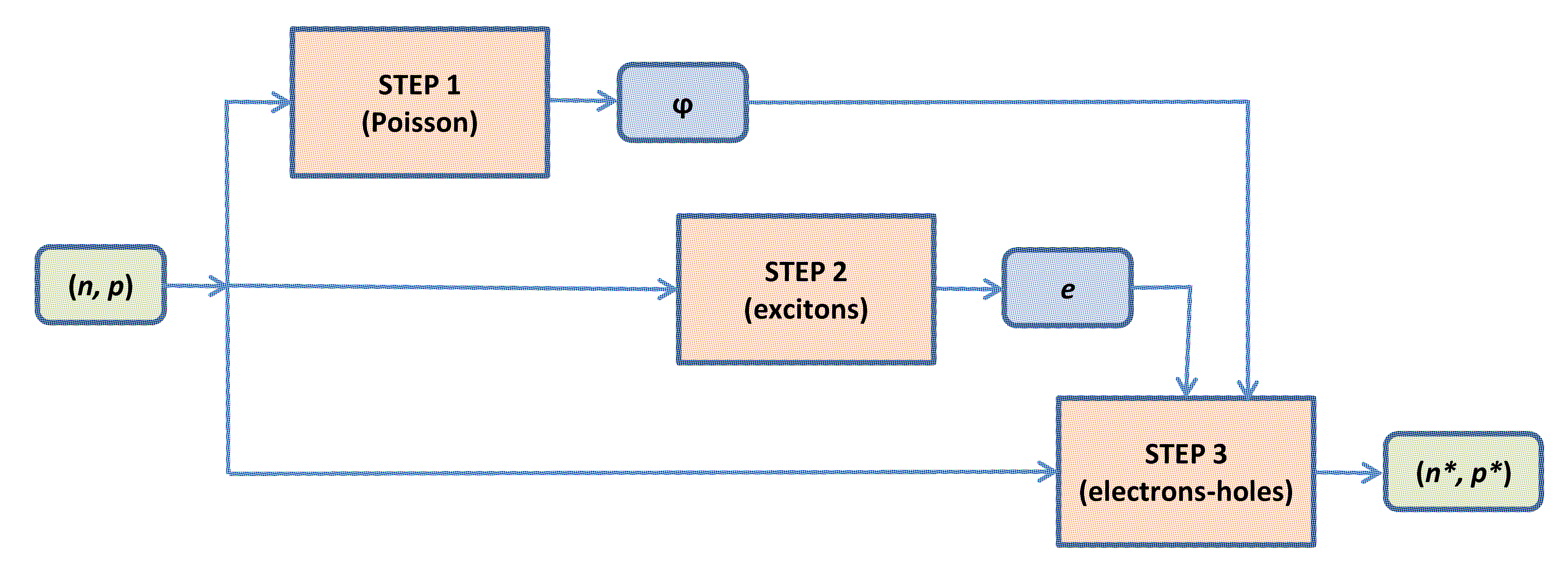
Figure 2. Flow-chart of the solution map.

STEP 1.:

Assume that $\left\{\Omega,\Gamma_{D},\Gamma_{N}\right\}$ is a $q-$admissible triple for some $q\geq 3$, $\varepsilon$ as specified in Tab. 2 and that there exists $\widetilde{\varphi}\in W^{1,q}\left(\Omega\right)$ whose trace on $\partial\Omega$ is equal to $\varphi_{D}$ on $\Gamma_{D}$. Take $g\left(\cdot\right)\equiv g\left(n\left(\cdot\right),p\left(\cdot\right)\right)$: then $g\left(\cdot\right)\in L^{q}\left(\Omega\right)$ by Lemma 18 so that there exists a unique weak solution $\varphi$ to the auxiliary Poisson problem (11). Moreover $\varphi\in W^{1,q}\left(\Omega\right)$ and for $i=n,p$, applying (16) and (46), we have

(48) $$\left\|\nabla\varphi\right\|_{L^{q}\left(\Omega_{i}\right)}\leq c\left(q,\Omega,\Gamma,\varepsilon\right)\left(R+\left\|\nabla\widetilde{\varphi}\right\|_{L^{q}\left(\Omega\right)}\right).$$

STEP 2.:

Assume $D_{e}$, $Q$, $H$, $\gamma$, $\tau_{e}$, $\tau_{d}$, $\eta$, $k_{d}$, $k_{r}$ to be as specified in Tab. 2. Take $f\left(\cdot\right)\equiv n\left(\cdot\right)p\left(\cdot\right)\geq 0$: then $f\left(\cdot\right)\in L^{2}\left(\Gamma\right)$ by Lemma 19. Let $e$ be the unique and nonnegative weak solution to the auxiliary exciton problem (22). Then, using (25), (47) and the fact that $\overline{\beta}=2\overline{h}\overline{\gamma}\eta$, we get

(49) $$\left\|e\right\|_{\mathcal{W}^{2}}\leq\frac{c\left(\Omega,\Gamma\right)}{\underline{d}_{e}}\left(\left\|Q\right\|_{L^{2}\left(\Omega\right)}+\overline{h}\overline{\gamma}\eta R^{2}\right).$$

STEP 3.:

Assume $D_{i}$, $\mu_{i}$, $i=n,p$, to be as specified in Tab. 2. Consider the auxiliary electron problem (31) where we take $\mu_{n}\left(\cdot\right)\equiv\mu_{n}\left(\cdot,\left|\nabla\varphi\left(\cdot\right)\right|\right)$, $h\left(\cdot\right)\equiv h\left(\cdot,p\left(\cdot\right)\right)\geq 0$, $h_{e}\left(\cdot\right)\equiv h_{e}\left(\cdot,e\left(\cdot\right)\right)\geq 0$. In particular it is $h\left(\cdot\right),h_{e}\left(\cdot\right)\in L^{2}\left(\Gamma\right)$ since $\beta,\omega\in L^{\infty}\left(\Gamma\right)$. Let $n^{\ast}$ be the unique and nonnegative weak solution to (31). Then, using (40), (30) and (24) we get

$$\left\|n^{\ast}\right\|_{\mathcal{W}_{n}^{2}}\leq\frac{c\left(\Omega_{n}\right)}{\Lambda_{n}}\left\|h_{e}\right\|_{L^{2}\left(\Gamma\right)}\leq\frac{\overline{h}c\left(\Omega_{n}\right)}{\tau_{d}\Lambda_{n}}\left\|e\right\|_{L^{2}\left(\Gamma\right)}\leq\frac{\overline{h}c\left(\Omega_{n}\right)}{\tau_{d}\Lambda_{n}}\left\|e\right\|_{\mathcal{W}^{2}}$$

and therefore, by (49),

(50) $$\left\|n^{\ast}\right\|_{\mathcal{W}_{n}^{2}}\leq c\left(\Omega,\Gamma\right)\frac{\overline{h}}{\underline{d}_{e}\tau_{d}\Lambda_{n}}\left(\left\|Q\right\|_{L^{2}\left(\Omega\right)}+\overline{h}\overline{\gamma}\eta R^{2}\right).$$

Applying similar arguments to the auxiliary hole problem (42) we obtain the following estimate for the function $p^{\ast}\geq 0$, unique and nonnegative weak solution to (42):

(51) $$\left\|p^{\ast}\right\|_{\mathcal{W}_{p}^{2}}\leq c\left(\Omega,\Gamma\right)\frac{\overline{h}}{\underline{d}_{e}\tau_{d}\Lambda_{p}}\left\{\left\|Q\right\|_{L^{2}\left(\Omega\right)}+\overline{h}\overline{\gamma}\eta R^{2}\right\}.$$

Remark 20.

From Lemmas 13 and 16 we know that $n^{\ast}$ and $p^{\ast}$ exist provided $\left\|\nabla\varphi\right\|_{L^{q}\left(\Omega_{i}\right)}<\delta$ ($i=n,p$) for a small enough $\delta$ or, equivalently, if $\Lambda_{n}>0$ and $\Lambda_{p}>0$.

6.3. The invariant set

In this section we seek a sufficient condition for $\mathbf{K}$ to act invariantly upon $\mathcal{B}_{R}^{+}$, i.e.

(52) $$\sqrt{\left\|n^{\ast}\right\|_{\mathcal{W}_{n}^{2}}^{2}+\left\|p^{\ast}\right\|_{\mathcal{W}_{p}^{2}}^{2}}\leq R.$$

Using (48) in (38) we get

$$\Lambda_{n}\geq\underline{d}_{n}-\overline{\mu}_{n}c\left(q,\Omega,\Gamma,\varepsilon\right)\left(R+\left\|\nabla\widetilde{\varphi}\right\|_{L^{q}\left(\Omega\right)}\right).$$

Set, for notational simplicity,

$$c_{0}:=c\left(q,\Omega,\Gamma,\varepsilon\right)$$

$$\underline{d}:=\min\left\{\underline{d}_{n};\underline{d}_{p}\right\}$$

$$\overline{\mu}:=\max\left\{\overline{\mu}_{n},\overline{\mu}_{p}\right\}$$

$$\overline{R}:=\frac{\underline{d}}{c_{0}\overline{\mu}}-\left\|\nabla\widetilde{\varphi}\right\|_{L^{q}\left(\Omega\right)}$$

Then

(53) $$\Lambda_{n}\geq\underline{d}-c_{0}\overline{\mu}\left(R+\left\|\nabla\widetilde{\varphi}\right\|_{L^{q}\left(\Omega\right)}\right)=c_{0}\overline{\mu}\left(\overline{R}-R\right).$$

Now assume $0<R<\overline{R}$ (so that $\Lambda_{n}>0$). Then by (50)

$$\left\|n^{\ast}\right\|_{\mathcal{W}_{n}^{2}}\leq\frac{c\left(\Omega,\Gamma\right)}{c_{0}}\frac{\overline{h}}{\underline{d}_{e}\tau_{d}\overline{\mu}}\frac{\left\|Q\right\|_{L^{2}\left(\Omega\right)}+\overline{h}\overline{\gamma}\eta R^{2}}{\overline{R}-R}.$$

A similar estimate holds for $\left\|p^{\ast}\right\|_{\mathcal{W}_{p}^{2}}$ so that

$$\sqrt{\left\|n^{\ast}\right\|_{\mathcal{W}_{n}^{2}}^{2}+\left\|p^{\ast}\right\|_{\mathcal{W}_{p}^{2}}^{2}}\leq c_{1}\frac{\overline{h}}{\underline{d}_{e}\tau_{d}\overline{\mu}}\frac{\left\|Q\right\|_{L^{2}\left(\Omega\right)}+\overline{h}\overline{\gamma}\eta R^{2}}{\overline{R}-R}$$

where $c_{1}=c_{1}\left(q,\Omega,\Gamma,\varepsilon\right)$. To satisfy (52) we have to require that

$$c_{1}\frac{\overline{h}}{\underline{d}_{e}\tau_{d}\overline{\mu}}\frac{\left\|Q\right\|_{L^{2}\left(\Omega\right)}+\overline{h}\overline{\gamma}\eta R^{2}}{\overline{R}-R}\leq R.$$

Write the above inequality as

(54) $$R^{2}-a\overline{R}R+ab\leq 0$$

where

(55) $$a:=\left(1+c_{1}\frac{\overline{h}^{2}\overline{\gamma}\eta}{\underline{d}_{e}\tau_{d}\overline{\mu}}\right)^{-1}\qquad;\qquad b:=c_{1}\frac{\overline{h}}{\underline{d}_{e}\tau_{d}\overline{\mu}}\left\|Q\right\|_{L^{2}\left(\Omega\right)}$$

Inequality (54) is solvable iff

$$\overline{R}\geq\sqrt{\frac{4b}{a}}$$

with solutions

(56) $$0<\underset{R_{1}}{\underbrace{\frac{a\overline{R}-\sqrt{a^{2}\overline{R}^{2}-4ab}}{2}}}\text{ }\leq R\leq\text{ }\underset{R_{2}}{\underbrace{\frac{a\overline{R}+\sqrt{a^{2}\overline{R}^{2}-4ab}}{2}}}.$$

In conclusion, the map $\mathbf{K}$ acts invariantly upon $\mathcal{B}_{R}^{+}$ (i.e., $\mathbf{K}\mathcal{B}_{R}^{+}\subset\mathcal{B}_{R}^{+}$) only for all the values of $R$ satisfying the set of conditions:

(57a) $$\overline{R}\geq\sqrt{\dfrac{4b}{a}}$$

(57b) $$0<R<\overline{R}$$

(57c) $$R_{1}\leq R\leq R_{2}.$$

Condition (57a) reads explicitly

(58) $$\left\|\nabla\widetilde{\varphi}\right\|_{L^{q}\left(\Omega\right)}+\sqrt{\dfrac{4c_{1}\overline{h}}{\underline{d}_{e}\tau_{d}\overline{\mu}}\left(1+\dfrac{c_{1}\overline{h}^{2}\overline{\gamma}\eta}{\underline{d}_{e}\tau_{d}\overline{\mu}}\right)\left\|Q\right\|_{L^{2}\left(\Omega\right)}}\leq\dfrac{\underline{d}}{c_{0}\overline{\mu}}$$

so it is certainly satisfied provided that

(59a) $$\left\|\nabla\widetilde{\varphi}\right\|_{L^{q}\left(\Omega\right)}\text{ and }\dfrac{\overline{h}}{\underline{d}_{e}\tau_{d}\overline{\mu}}\left\|Q\right\|_{L^{2}\left(\Omega\right)}\text{ are small enough, or}$$

(59b) $$\dfrac{\,\underline{d}\,}{\overline{\mu}}\text{ is large enough.}$$

From (54) and the fact that $0<a<1$ it follows that

$$0<R_{1}\leq R_{2}<R_{1}+R_{2}=a\overline{R}<\overline{R}$$

which implies that (57c) is more restrictive than (57b). We have thus proved the following result.

Proposition 21 (Existence of an invariant set for $\mathbf{K}$).

Let $\mathbf{K}:\mathcal{B}_{R}^{+}\longrightarrow\mathcal{W}_{n}^{2}\oplus\mathcal{W}_{p}^{2}$ be the map $\left(n^{\ast},p^{\ast}\right)=\mathbf{K}\left(n,p\right)$ defined through Steps 1-3. Assume that (59) holds. Then $\mathbf{K}\mathcal{B}_{R}^{+}\subset\mathcal{B}_{R}^{+}$ for all $R$ satisfying $R_{1}\leq R\leq R_{2}$, where the values of $R_{1}$ and $R_{2}$ are given in (56).

6.4. Fixed-point by contraction

The goal of this section is to prove that $\mathbf{K}$ is a strict contraction mapping of $\mathcal{B}_{R}^{+}$ into itself. This ensures that $\mathbf{K}$ admits a unique fixed point. Let $\left(n_{i},p_{i}\right)\in\mathcal{B}_{R}^{+}$ and $\left(n_{i}^{\ast},p_{i}^{\ast}\right)=\mathbf{K}\left(n_{i},p_{i}\right)$ ($i=1,2$): then we seek a constant $\lambda\in\left(0,1\right)$ such that

(60) $$\sqrt{\left\|n_{2}^{\ast}-n_{1}^{\ast}\right\|_{\mathcal{W}_{n}^{2}}^{2}+\left\|p_{2}^{\ast}-p_{1}^{\ast}\right\|_{\mathcal{W}_{p}^{2}}^{2}}\leq\lambda\sqrt{\left\|n_{2}-n_{1}\right\|_{\mathcal{W}_{n}^{2}}^{2}+\left\|p_{2}-p_{1}\right\|_{\mathcal{W}_{p}^{2}}^{2}}.$$

Lemma 22.

Let $\left(n_{i},p_{i}\right)\in\mathcal{B}_{R}^{+}$ and

(61) $$g\left(\cdot\right)=g\left(n_{2},p_{2}\right)-g\left(n_{1},p_{1}\right)=\left\{\begin{array}[]{ll}-\left(n_{2}-n_{1}\right)&\text{in \ }\Omega_{n}\\ p_{2}-p_{1}&\text{in }\Omega_{p}.\end{array}\right.$$

Then $g\in L^{q}\left(\Omega\right)$ for $2\leq q\leq 6$ and there exists a constant $c=c\left(q,\Omega,\Gamma\right)$ such that

(62) $$\left\|g\right\|_{L^{q}\left(\Omega\right)}\leq c\sqrt{\left\|n_{2}-n_{1}\right\|_{\mathcal{W}_{n}^{2}}^{2}+\left\|p_{2}-p_{1}\right\|_{\mathcal{W}_{p}^{2}}^{2}}.$$

Proof.

Proceeding as in the proof of Lemma 18 we have

$$\left\|g\right\|_{L^{q}\left(\Omega\right)}^{q} \leq c\left(q,\Omega_{n}\right)\left\|n_{2}-n_{1}\right\|_{\mathcal{W}_{n}^{2}}^{q}+c\left(q,\Omega_{p}\right)\left\|p_{2}-p_{1}\right\|_{\mathcal{W}_{p}^{2}}^{q}$$

$$\leq c\left(q,\Omega,\Gamma\right)\left(\left\|n_{2}-n_{1}\right\|_{\mathcal{W}_{n}^{2}}^{q}+\left\|p_{2}-p_{1}\right\|_{\mathcal{W}_{p}^{2}}^{q}\right).$$

Then the assertion follows from the inequality

$$\left(a^{q}+b^{q}\right)^{1/q}\leq\left(a^{2}+b^{2}\right)^{1/2}$$

with $a>0$, $b>0$, $q\geq 2$. ∎

Lemma 23.

Let $\left(n_{i},p_{i}\right)\in\mathcal{B}_{R}^{+}$ and

(63) $$f\left(\cdot\right)=n_{2}p_{2}-n_{1}p_{1}$$

Then $f\in L^{2}\left(\Gamma\right)$ and there exists a constant $c=c\left(\Omega,\Gamma\right)$ such that

(64) $$\left\|f\right\|_{L^{2}\left(\Gamma\right)}\leq cR\sqrt{\left\|n_{2}-n_{1}\right\|_{\mathcal{W}_{n}^{2}}^{2}+\left\|p_{2}-p_{1}\right\|_{\mathcal{W}_{p}^{2}}^{2}}$$

Proof.

We have

$$n_{2}p_{2}-n_{1}p_{1}=p_{2}\left(n_{2}-n_{1}\right)+n_{1}\left(p_{2}-p_{1}\right)$$

so that, by (24) (where $\mathcal{W}^{2}$ is substituted by $\mathcal{W}_{p}^{2}$ and $\mathcal{W}_{n}^{2}$), we obtain

$$\left\|f\right\|_{L^{2}\left(\Gamma\right)} \leq \left\|p_{2}\left(n_{2}-n_{1}\right)\right\|_{L^{2}\left(\Gamma\right)}+\left\|n_{1}\left(p_{2}-p_{1}\right)\right\|_{L^{2}\left(\Gamma\right)}$$

$$\leq \left\|p_{2}\right\|_{L^{4}\left(\Gamma\right)}\left\|n_{2}-n_{1}\right\|_{L^{4}\left(\Gamma\right)}+\left\|n_{1}\right\|_{L^{4}\left(\Gamma\right)}\left\|p_{2}-p_{1}\right\|_{L^{4}\left(\Gamma\right)}$$

$$\leq c\left(\Omega,\Gamma\right)\left(\left\|p_{2}\right\|_{\mathcal{W}_{p}^{2}}\left\|n_{2}-n_{1}\right\|_{\mathcal{W}_{n}^{2}}+\left\|n_{1}\right\|_{\mathcal{W}_{n}^{2}}\left\|p_{2}-p_{1}\right\|_{\mathcal{W}_{p}^{2}}\right)$$

$$\leq c\left(\Omega,\Gamma\right)R\sqrt{\left\|n_{2}-n_{1}\right\|_{\mathcal{W}_{n}^{2}}^{2}+\left\|p_{2}-p_{1}\right\|_{\mathcal{W}_{p}^{2}}^{2}}.$$

∎

Given $\left(n_{i},p_{i}\right)\in\mathcal{B}_{R}^{+}$, $i=1,2$, we call $\varphi_{i}=u_{i}+\widetilde{\varphi}$ and $e_{i}$ the corresponding functions computed by Steps 1 and 2, respectively. Each of the $u_{i}$’s satisfies problem (13) so that, taking the difference, we obtain

(65) $$a\left(u_{2}-u_{1},v\right)=\int_{\Omega}\left(g\left(n_{2},p_{2}\right)-g\left(n_{1},p_{1}\right)\right)v\,dx$$

Problem (65) looks like the auxiliary Poisson problem (see Lemma 7 where $g$ is given by (61) and $\widetilde{\varphi}=0$), hence by (15) and (62) we have

$$\left\|u_{2}-u_{1}\right\|_{\mathcal{W}^{q}}\leq c\left(q,\Omega,\Gamma,\varepsilon\right)\sqrt{\left\|n_{2}-n_{1}\right\|_{\mathcal{W}_{n}^{2}}^{2}+\left\|p_{2}-p_{1}\right\|_{\mathcal{W}_{p}^{2}}^{2}}.$$

In particular: $u_{2}-u_{1}=\left(\varphi_{2}-\widetilde{\varphi}\right)-\left(\varphi_{1}-\widetilde{\varphi}\right)=\varphi_{2}-\varphi_{1}$ and

(66) $$\left\|\nabla\varphi_{2}-\nabla\varphi_{1}\right\|_{L^{q}\left(\Omega\right)}\leq c\left(q,\Omega,\Gamma,\varepsilon\right)\sqrt{\left\|n_{2}-n_{1}\right\|_{\mathcal{W}_{n}^{2}}^{2}+\left\|p_{2}-p_{1}\right\|_{\mathcal{W}_{p}^{2}}^{2}}.$$

Let us now consider the $e_{i}$’s. Each of them satisfies problem (23), so that

(67) $$b\left(e_{2}-e_{1},v\right)=\int_{\Gamma}\beta\left(\cdot\right)\left(n_{2}p_{2}-n_{1}p_{1}\right)v\,d\sigma.$$

Problem (67) looks like the auxiliary exciton problem (see Lemma 10 where $f$ is given by (63) and $Q=0$), hence by (25) and (64) we have

(68) $$\left\|e_{2}-e_{1}\right\|_{\mathcal{W}^{2}}\leq\frac{c\left(\Omega,\Gamma\right)\overline{\beta}R}{\underline{d}_{e}}\sqrt{\left\|n_{2}-n_{1}\right\|_{\mathcal{W}_{n}^{2}}^{2}+\left\|p_{2}-p_{1}\right\|_{\mathcal{W}_{p}^{2}}^{2}}.$$

Now we need the following assumption: the drift velocities $\mu_{i}\left(\cdot,E\right)\mathbf{E}$ ($i=n,p$) are Lipschitzian with respect to $\mathbf{E}$, namely

(69a) $$\left|\mu_{i}\left(\cdot,E_{2}\right)\mathbf{E}_{2}-\mu_{i}\left(\cdot,E_{1}\right)\mathbf{E}_{1}\right|\leq\mu_{i,0}\left(\cdot\right)\left|\mathbf{E}_{2}-\mathbf{E}_{1}\right|$$

where

(69b) $$0\leq\mu_{i,0}\left(\cdot\right)\in L^{\infty}\left(\Omega_{i}\right).$$

Remark 24.

Assumption (69) is trivially satisfied if $\mu_{i}\left(\cdot,E\right)\equiv\mu_{i,0}\left(\cdot\right)\in L^{\infty}\left(\Omega_{i}\right)$. It is also satisfied by the model proposed in [30], i.e. the functions $\mu_{i}\left(\mathbf{x},\cdot\right)$ enjoy the conditions stated in Tab. 2 and, in addition, they are Lipschitzian ($L_{i}\in L^{\infty}\left(\Omega_{i}\right)$)

$$\left|\mu_{i}\left(\cdot,E_{2}\right)-\mu_{i}\left(\cdot,E_{1}\right)\right|\leq L_{i}\left(\cdot\right)\left|E_{2}-E_{1}\right|$$

and there exists a cutoff field $E^{\ast}$ above which $\mu_{i}\left(\mathbf{x},\cdot\right)\equiv\mu_{i,0}\left(\mathbf{x}\right)$. As a matter of fact, for $0\leq E_{1}<E_{2}$, we have

$$\left|\mu_{i}\left(\cdot,E_{2}\right)\mathbf{E}_{2}-\mu_{i}\left(\cdot,E_{1}\right)\mathbf{E}_{1}\right| = \left|\mu_{i}\left(\cdot,E_{2}\right)\left(\mathbf{E}_{2}-\mathbf{E}_{1}\right)+\left(\mu_{i}\left(\cdot,E_{2}\right)-\mu_{i}\left(\cdot,E_{1}\right)\right)\mathbf{E}_{1}\right|$$

$$\leq \mu_{i}\left(\cdot,E_{2}\right)\left|\mathbf{E}_{2}-\mathbf{E}_{1}\right|+\left|\mu_{i}\left(\cdot,E_{2}\right)-\mu_{i}\left(\cdot,E_{1}\right)\right|E_{1}.$$

Let $E^{\ast}\leq E_{1}$. Then $\mu_{i}\left(\cdot,E_{1}\right)=\mu_{i}\left(\cdot,E_{2}\right)=\mu_{i,0}\left(\cdot\right)$ so that (69) are obtained. On the other hand, if $E_{1}\leq E^{\ast}$, we have

$$\left|\mu_{i}\left(\cdot,E_{2}\right)\mathbf{E}_{2}-\mu_{i}\left(\cdot,E_{1}\right)\mathbf{E}_{1}\right| \leq \overline{\mu}_{i}\left|\mathbf{E}_{2}-\mathbf{E}_{1}\right|+L_{i}\left(\cdot\right)\left|E_{2}-E_{1}\right|E^{\ast}$$

$$\leq \left(\overline{\mu}_{i}+L_{i}\left(\cdot\right)\right)\left|\mathbf{E}_{2}-\mathbf{E}_{1}\right|$$

since $\left|E_{2}-E_{1}\right|\leq\left|\mathbf{E}_{2}-\mathbf{E}_{1}\right|$, and (69) are again obtained.

Let us now consider the outputs of the solution map, $\left(n_{i}^{\ast},p_{i}^{\ast}\right)$, $i=1,2$. Each of the $n_{i}^{\ast}$’s satisfies problem (32), so that

$$\int_{\Omega_{n}}D_{n}\left(\cdot\right)\nabla n_{i}^{\ast}\cdot\nabla vdx-\int_{\Omega_{n}}\mu_{n}\left(\cdot,\left|\nabla\varphi_{i}\right|\right)n_{i}^{\ast}\nabla\varphi_{i}\cdot\nabla vdx+\eta^{-1}\int_{\Gamma}\beta\left(\cdot\right)p_{i}n_{i}^{\ast}vd\sigma=\int_{\Gamma}\omega\left(\cdot\right)e_{i}vd\sigma$$

Setting $\mu_{i}\left(\cdot\right)\equiv\mu_{n}\left(\cdot,\left|\nabla\varphi_{i}\right|\right)$ for brevity and subtracting $i=1$ from $i=2$, we obtain

$$\int_{\Omega_{n}}D_{n}\left(\cdot\right)\nabla\left(n_{2}^{\ast}-n_{1}^{\ast}\right)\cdot\nabla vdx+\eta^{-1}\int_{\Gamma}\beta\left(\cdot\right)\left(p_{2}n_{2}^{\ast}-p_{1}n_{1}^{\ast}\right)vd\sigma$$

$$=\int_{\Omega_{n}}\left(n_{2}^{\ast}\mu_{2}\left(\cdot\right)\nabla\varphi_{2}-n_{1}^{\ast}\mu_{1}\left(\cdot\right)\nabla\varphi_{1}\right)\cdot\nabla vdx+\int_{\Gamma}\omega\left(\cdot\right)\left(e_{2}-e_{1}\right)vd\sigma.$$

Choose $v=n_{2}^{\ast}-n_{1}^{\ast}$ and use the identity

$$p_{2}n_{2}^{\ast}-p_{1}n_{1}^{\ast}=p_{2}\left(n_{2}^{\ast}-n_{1}^{\ast}\right)+\left(p_{2}-p_{1}\right)n_{1}^{\ast}.$$

Then

$$\int_{\Omega_{n}}D_{n}\left(\cdot\right)\left|\nabla\left(n_{2}^{\ast}-n_{1}^{\ast}\right)\right|^{2}dx+\eta^{-1}\int_{\Gamma}\beta\left(\cdot\right)p_{2}\left(n_{2}^{\ast}-n_{1}^{\ast}\right)^{2}d\sigma$$

$$= \int_{\Omega_{n}}\left(n_{2}^{\ast}\mu_{2}\left(\cdot\right)\nabla\varphi_{2}-n_{1}^{\ast}\mu_{1}\left(\cdot\right)\nabla\varphi_{1}\right)\cdot\nabla\left(n_{2}^{\ast}-n_{1}^{\ast}\right)dx$$

$$-\eta^{-1}\int_{\Gamma}\beta\left(\cdot\right)\left(p_{2}-p_{1}\right)n_{1}^{\ast}\left(n_{2}^{\ast}-n_{1}^{\ast}\right)d\sigma+\int_{\Gamma}\omega\left(\cdot\right)\left(e_{2}-e_{1}\right)\left(n_{2}^{\ast}-n_{1}^{\ast}\right)d\sigma$$

from which it follows

(70) $$\underline{d}\left\|n_{2}^{\ast}-n_{1}^{\ast}\right\|_{\mathcal{W}_{n}^{2}}^{2} \leq \int_{\Omega_{n}}D_{n}\left(\cdot\right)\left|\nabla\left(n_{2}^{\ast}-n_{1}^{\ast}\right)\right|^{2}dx+\eta^{-1}\int_{\Gamma}\beta\left(\cdot\right)p_{2}\left(n_{2}^{\ast}-n_{1}^{\ast}\right)^{2}d\sigma$$

$$\leq \int_{\Omega_{n}}\left|n_{2}^{\ast}\mu_{2}\left(\cdot\right)\nabla\varphi_{2}-n_{1}^{\ast}\mu_{1}\left(\cdot\right)\nabla\varphi_{1}\right|\left|\nabla\left(n_{2}^{\ast}-n_{1}^{\ast}\right)\right|dx$$

$$+\eta^{-1}\overline{\beta}\int_{\Gamma}\left|\left(p_{2}-p_{1}\right)n_{1}^{\ast}\left(n_{2}^{\ast}-n_{1}^{\ast}\right)\right|d\sigma+\overline{\alpha}\int_{\Gamma}\left|\left(e_{2}-e_{1}\right)\left(n_{2}^{\ast}-n_{1}^{\ast}\right)\right|d\sigma$$

$$= I_{1}+\eta^{-1}\overline{\beta}I_{2}+\overline{\alpha}I_{3}.$$

Use of the identity

$$n_{2}^{\ast}\mu_{2}\nabla\varphi_{2}-n_{1}^{\ast}\mu_{1}\nabla\varphi_{1}=n_{2}^{\ast}\left(\mu_{2}\nabla\varphi_{2}-\mu_{1}\nabla\varphi_{1}\right)+\left(n_{2}^{\ast}-n_{1}^{\ast}\right)\mu_{1}\nabla\varphi_{1}$$

gives

$$I_{1} \leq \int_{\Omega_{n}}\left|n_{2}^{\ast}\left(\mu_{2}\nabla\varphi_{2}-\mu_{1}\nabla\varphi_{1}\right)\right|\left|\nabla\left(n_{2}^{\ast}-n_{1}^{\ast}\right)\right|dx$$

$$+ \int_{\Omega_{n}}\left|\left(n_{2}^{\ast}-n_{1}^{\ast}\right)\mu_{1}\nabla\varphi_{1}\right|\left|\nabla\left(n_{2}^{\ast}-n_{1}^{\ast}\right)\right|dx=J_{1}+J_{2}$$

But

$$J_{1}\leq\left\|n_{2}^{\ast}\right\|_{L^{r}\left(\Omega_{n}\right)}\left\|\mu_{2}\nabla\varphi_{2}-\mu_{1}\nabla\varphi_{1}\right\|_{L^{q}\left(\Omega_{n}\right)}\left\|\nabla\left(n_{2}^{\ast}-n_{1}^{\ast}\right)\right\|_{L^{2}\left(\Omega_{n}\right)}$$

where $1/r+1/q=1/2$ (see (34)). We have

$$\left\|n_{2}^{\ast}\right\|_{L^{r}\left(\Omega_{n}\right)}\leq c\left(q,\Omega_{n}\right)\left\|n_{2}^{\ast}\right\|_{\mathcal{W}_{n}^{2}}\leq c\left(q,\Omega_{n}\right)R$$

(see (35)) and, by (69) and (66),

$$\left\|\mu_{2}\nabla\varphi_{2}-\mu_{1}\nabla\varphi_{1}\right\|_{L^{q}\left(\Omega_{n}\right)} \leq \overline{\mu}\left\|\nabla\varphi_{2}-\nabla\varphi_{1}\right\|_{L^{q}\left(\Omega_{n}\right)}$$

$$\leq c\left(q,\Omega,\Gamma,\varepsilon\right)\overline{\mu}\sqrt{\left\|n_{2}-n_{1}\right\|_{\mathcal{W}_{n}^{2}}^{2}+\left\|p_{2}-p_{1}\right\|_{\mathcal{W}_{p}^{2}}^{2}}.$$

Finally, the application of (2) with $i=n$ and $q=2$ gives

$$\left\|\nabla\left(n_{2}^{\ast}-n_{1}^{\ast}\right)\right\|_{L^{2}\left(\Omega_{n}\right)}=\left\|n_{2}^{\ast}-n_{1}^{\ast}\right\|_{\mathcal{W}_{n}^{2}}.$$

Collecting the above estimates, we obtain

$$J_{1}\leq c\left(q,\Omega,\Gamma,\varepsilon\right)\overline{\mu}R\sqrt{\left\|n_{2}-n_{1}\right\|_{\mathcal{W}_{n}^{2}}^{2}+\left\|p_{2}-p_{1}\right\|_{\mathcal{W}_{p}^{2}}^{2}}\left\|n_{2}^{\ast}-n_{1}^{\ast}\right\|_{\mathcal{W}_{n}^{2}}.$$

Similarly,

$$J_{2} \leq \overline{\mu}\int_{\Omega_{n}}\left|\left(n_{2}^{\ast}-n_{1}^{\ast}\right)\nabla\varphi_{1}\right|\left|\nabla\left(n_{2}^{\ast}-n_{1}^{\ast}\right)\right|dx$$

$$\leq \overline{\mu}\left\|n_{2}^{\ast}-n_{1}^{\ast}\right\|_{L^{r}\left(\Omega_{n}\right)}\left\|\nabla\varphi_{1}\right\|_{L^{q}\left(\Omega_{n}\right)}\left\|\nabla\left(n_{2}^{\ast}-n_{1}^{\ast}\right)\right\|_{L^{2}\left(\Omega_{n}\right)}$$

$$\leq \overline{\mu}c\left(q,\Omega_{n}\right)\left\|\nabla\varphi_{1}\right\|_{L^{q}\left(\Omega_{n}\right)}\left\|n_{2}^{\ast}-n_{1}^{\ast}\right\|_{\mathcal{W}_{n}^{2}}^{2}.$$

Moreover, we have

$$I_{2} = \int_{\Gamma}\left|\left(p_{2}-p_{1}\right)n_{1}^{\ast}\left(n_{2}^{\ast}-n_{1}^{\ast}\right)\right|d\sigma$$

$$\leq \left\|n_{1}^{\ast}\right\|_{L^{4}\left(\Gamma\right)}\left\|p_{2}-p_{1}\right\|_{L^{4}\left(\Gamma\right)}\left\|n_{2}^{\ast}-n_{1}^{\ast}\right\|_{L^{2}\left(\Gamma\right)}$$

$$\leq \left\|n_{1}^{\ast}\right\|_{L^{4}\left(\partial\Omega_{n}\right)}\left\|p_{2}-p_{1}\right\|_{L^{4}\left(\partial\Omega_{p}\right)}\left\|n_{2}^{\ast}-n_{1}^{\ast}\right\|_{L^{2}\left(\partial\Omega_{n}\right)}$$

$$\leq c\left(\Omega,\Gamma\right)\left\|n_{1}^{\ast}\right\|_{H^{1}\left(\Omega_{n}\right)}\left\|p_{2}-p_{1}\right\|_{H^{1}\left(\Omega_{p}\right)}\left\|n_{2}^{\ast}-n_{1}^{\ast}\right\|_{H^{1}\left(\Omega_{n}\right)}$$

$$\leq c\left(\Omega,\Gamma\right)\left\|n_{1}^{\ast}\right\|_{\mathcal{W}_{n}^{2}}\left\|p_{2}-p_{1}\right\|_{\mathcal{W}_{p}^{2}}\left\|n_{2}^{\ast}-n_{1}^{\ast}\right\|_{\mathcal{W}_{n}^{2}}$$

$$\leq c\left(\Omega,\Gamma\right)R\sqrt{\left\|n_{2}-n_{1}\right\|_{\mathcal{W}_{n}^{2}}^{2}+\left\|p_{2}-p_{1}\right\|_{\mathcal{W}_{p}^{2}}^{2}}\left\|n_{2}^{\ast}-n_{1}^{\ast}\right\|_{\mathcal{W}_{n}^{2}}$$

and, using (30), (24) and (68),

$$I_{3} = \int_{\Gamma}\left|\left(e_{2}-e_{1}\right)\left(n_{2}^{\ast}-n_{1}^{\ast}\right)\right|d\sigma\leq\left\|e_{2}-e_{1}\right\|_{L^{2}\left(\Gamma\right)}\left\|n_{2}^{\ast}-n_{1}^{\ast}\right\|_{L^{2}\left(\Gamma\right)}$$

$$\leq c\left(\Omega,\Gamma\right)\left\|e_{2}-e_{1}\right\|_{\mathcal{W}^{2}}\left\|n_{2}^{\ast}-n_{1}^{\ast}\right\|_{\mathcal{W}_{n}^{2}}$$

$$\leq \frac{c\left(\Omega,\Gamma\right)\overline{\beta}R}{\underline{d}_{e}}\sqrt{\left\|n_{2}-n_{1}\right\|_{\mathcal{W}_{n}^{2}}^{2}+\left\|p_{2}-p_{1}\right\|_{\mathcal{W}_{p}^{2}}^{2}}\left\|n_{2}^{\ast}-n_{1}^{\ast}\right\|_{\mathcal{W}_{n}^{2}}.$$

Inserting the obtained estimates for $I_{1}$, $I_{2}$ and $I_{3}$ into (70) yields

$$\left(\underline{d}-c\left(q,\Omega,\Gamma,\varepsilon\right)\overline{\mu}\left\|\nabla\varphi_{1}\right\|_{L^{q}\left(\Omega_{n}\right)}\right)\left\|n_{2}^{\ast}-n_{1}^{\ast}\right\|_{\mathcal{W}_{n}^{2}}$$

$$\leq\left(\overline{\mu}c\left(q,\Omega,\Gamma,\varepsilon\right)+\left(\frac{\overline{\beta}}{\eta}+\frac{\overline{\alpha}\overline{\beta}}{\underline{d}_{e}}\right)c\left(\Omega,\Gamma\right)\right)R\sqrt{\left\|n_{2}-n_{1}\right\|_{\mathcal{W}_{n}^{2}}^{2}+\left\|p_{2}-p_{1}\right\|_{\mathcal{W}_{p}^{2}}^{2}}$$

But using (48) gives

$$\underline{d}-\overline{\mu}c\left(q,\Omega,\Gamma,\varepsilon\right)\left\|\nabla\varphi_{1}\right\|_{L^{q}\left(\Omega_{n}\right)}\geq\underline{d}-\overline{\mu}c\left(q,\Omega,\Gamma,\varepsilon\right)\left(R+\left\|\nabla\widetilde{\varphi}\right\|_{L^{q}\left(\Omega\right)}\right)=c_{0}\overline{\mu}\left(\overline{R}-R\right)$$

where $c_{0}$ can be chosen as in (38) without loss of generality. Then

$$\left\|n_{2}^{\ast}-n_{1}^{\ast}\right\|_{\mathcal{W}_{n}^{2}}\leq\left(1+\left(\frac{\overline{\beta}}{\overline{\mu}\eta}+\frac{\overline{\alpha}\overline{\beta}}{\overline{\mu}\underline{d}_{e}}\right)c_{1}\right)\frac{R}{\overline{R}-R}\sqrt{\left\|n_{2}-n_{1}\right\|_{\mathcal{W}_{n}^{2}}^{2}+\left\|p_{2}-p_{1}\right\|_{\mathcal{W}_{p}^{2}}^{2}}$$

where $c_{1}$ can be chosen as in (55). A similar estimate can be proved to hold also for $\left\|p_{2}^{\ast}-p_{1}^{\ast}\right\|_{\mathcal{W}_{p}^{2}}$, so that, in conclusion, we get (60) where

$$\lambda=\frac{\widehat{c}R}{\overline{R}-R}$$

having set

$$\widehat{c}:=\sqrt{2}\left(1+c_{1}\frac{\overline{\beta}}{\overline{\mu}}\left(\frac{1}{\eta}+\frac{\overline{\alpha}}{\underline{d}_{e}}\right)\right).$$

By Proposition 21 we know that $0<R_{1}\leq R\leq R_{2}<\overline{R}$. Now, it is $0<\lambda<1$ if and only if

$$0<R<\frac{\overline{R}}{1+\widehat{c}}<\overline{R}$$

so that the map $\mathbf{K}$ is a contraction provided that

$$R_{1}<\frac{\overline{R}}{1+\widehat{c}}$$

i.e.

(71) $$\underset{=\text{ }\widehat{a}}{\underbrace{\left(a-\frac{2}{1+\widehat{c}}\right)}}\,\overline{R}<\sqrt{a^{2}\overline{R}^{2}-4ab}.$$

Two cases are in order:

• if $\widehat{a}\leq 0$, then condition (71) is satisfied, hence under condition (58) the map $\mathbf{K}:\mathcal{B}_{R}^{+}\longrightarrow\mathcal{B}_{R}^{+}$ is a contraction for all $R$ satisfying $R_{1}\leq R<\min\left\{R_{2};\frac{\overline{R}}{1+\widehat{c}}\right\}$;

• if $\widehat{a}>0$, then condition (71) reads

  (72) $$\overline{R}>\sqrt{\frac{4ab}{a^{2}-\widehat{a}^{2}}}=\frac{1}{\sqrt{1-\left(\dfrac{\widehat{a}}{a}\right)^{2}}}\sqrt{\dfrac{4b}{a}}$$

  which is stronger than condition (57a) since $\widehat{a}<a$. Moreover, in this case it is always $\dfrac{\overline{R}}{1+\widehat{c}}<R_{2}$. Therefore: under condition (72) the map $\mathbf{K}:\mathcal{B}_{R}^{+}\longrightarrow\mathcal{B}_{R}^{+}$ is a contraction for all $R$ satisfying $R_{1}\leq R<\frac{\overline{R}}{1+\widehat{c}}$.

Condition (72) can be written as $\overline{R}>\sigma\sqrt{\dfrac{4b}{a}}$ with $\sigma>1$ and it reads explicitly

(73) $$\left\|\nabla\widetilde{\varphi}\right\|_{L^{q}\left(\Omega\right)}+\sigma\sqrt{\dfrac{4c_{1}\overline{h}}{\underline{d}_{e}\tau_{d}\overline{\mu}}\left(1+\dfrac{c_{1}\overline{h}^{2}\overline{\gamma}\eta}{\underline{d}_{e}\tau_{d}\overline{\mu}}\right)\left\|Q\right\|_{L^{2}\left(\Omega\right)}}<\dfrac{\underline{d}}{c_{0}\overline{\mu}}$$

to be compared with (58). Both (58) and (73) are satisfied under condition (59).

We have thus proved the following result.

Theorem 25.

Let $\mathbf{K}:\mathcal{B}_{R}^{+}\longrightarrow\mathcal{W}_{n}^{2}\oplus\mathcal{W}_{p}^{2}$ be the map $\left(n^{\ast},p^{\ast}\right)=\mathbf{K}\left(n,p\right)$ defined through Steps 1-3. In addition, assume that (59) and (69) hold. Then there exist $R_{2}>R_{1}>0$ such that $\mathbf{K}\mathcal{\ }$is a strict contraction on $\mathcal{B}_{R}^{+}$ for all $R$ satisfying $R_{1}<R<R_{2}$. Thus, $\mathbf{K}$ admits a unique fixed point in $\mathcal{B}_{R}^{+}$.

7. Solution map validation through numerical simulation

In this section we carry out a computational validation of the theoretical properties of the fixed-point map introduced and analyzed in Sect. 6. To this purpose, we consider the realistic three-dimensional solar cell geometry shown in Fig. 3 which represents the unit cell of an ideal lattice of chessboard-shaped nanostructures of donor and acceptor materials.

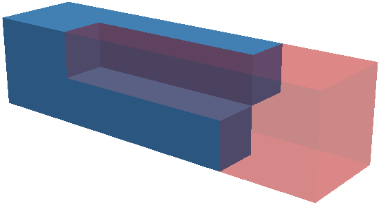
Figure 3. Simulation domain scheme (a) and 3D representation (b).

The whole cell domain is obtained by symmetrically repeating the module of Fig. 3 with respect to the lateral faces on the part of the boundary denoted with $\Gamma_{N}=\partial\Omega\setminus(\Gamma_{C}\cup\Gamma_{A})$ in Fig. 3. Since $\Omega$ is a convex polyhedron and the border between $\Gamma_{D}$ and $\Gamma_{N}$ consists of a finite number of segments, then the triple $\left\{\Omega,\Gamma_{D},\Gamma_{N}\right\}$ associated with the geometry depicted in Fig. 3 is $q-$admissible for a $q>3$ (see [6, 18, 19]).

The electrochemical behaviour of the cell can be described by equations (3)-(7) enforcing symmetry conditions on $\Gamma_{N}$, i.e. applying zero-flux conditions. The iterative map illustrated in Sect. 6 is then applied to the model equations that are numerically solved upon using a suitable finite element discretization scheme.

According to the theoretical results of Theorem 25, the map should converge to a unique fixed point if conditions (59) and (69) are met. In particular we analyzed the behaviour of the map by systematically changing the value of:

• the exciton photogeneration term $Q$;

• the electron and hole mobilities $\mu_{n}$ and $\mu_{p}$;

• the voltage $\varphi_{C}-\varphi_{A}$ applied to the electrodes.

Conditions (59) suggest that there might be particular threshold values for such parameters above or below which the convergence of the map is compromised. We want to investigate whether such values exist and to study the dependence of the convergence speed of the map on the value attained by such parameters.

The following assumptions are made on the functional form of the model parameters:

1. The light absorption is uniform through the entire cell, i.e. $Q(\mathbf{x})=Q$;

2. Electron and hole mobility parameters $\mu_{n}$ and $\mu_{p}$ depend on the local electric field according to the functional form ($i=n,p$)

   (74) $$\mu_{i}\left(E\right)=\left\{\begin{tabular}[]{lll}$\mu_{i,0}\exp\left(\dfrac{\beta_{i}\sqrt{E}}{k_{B}T}\right)$&if&$E<E^{\ast}$\\ $\mu_{i,0}\exp\left(\dfrac{\beta_{i}\sqrt{E^{\ast}}}{k_{B}T}\right)$&if&$E\geq E^{\ast}$\end{tabular}\right.$$

   where $E$ is the electric field intensity, $\mu_{i,0}$ is the zero-field mobility of the charge carrier, $\beta_{i}$ is a modulation parameter, $K_{B}$ is the Boltzmann constant and $T$ is the temperature. Definition (74) is a modified version of a model widely used in the literature, see e.g. [2, 3, 22, 31, 32], where the ceiling for values of $E$ above the cutoff level $E^{\ast}$ has been introduced to be consistent with the assumptions reported in Tab. 2.

3. Electron and hole diffusion coefficients have been assumed to be constant consistently with the assumptions of Tab. 2 and given by

   (75) $$D_{i}=\dfrac{k_{B}T}{q}\ \dfrac{\mu_{i}\left(0\right)+\mu_{i}\left(E^{\ast}\right)}{2}$$

   where $q$ denotes the elementary electric charge. The second term at the right-hand side of (75) represents the average between the value of the mobility at zero electric field and that at the cutoff level $E^{\ast}$ introduced in (74).

4. The bimolecular recombination rate $\gamma$ is defined with the formula described in [28, 2] with the dependence on the electric field removed to be compliant with the assumption made in Tab. 2, i.e.

   (76) $$\gamma=\dfrac{q}{\varepsilon^{\ast}}\min\left\{\mu_{n,0};\mu_{p,0}\right\}$$

   where $\varepsilon^{\ast}$ is defined as the harmonic average of the dielectric permittivities of the acceptor and donor materials

   (77) $$\varepsilon^{\ast}=\left(\dfrac{\varepsilon_{\mathrm{acc}}^{-1}+\varepsilon_{\mathrm{don}}^{-1}}{2}\right)^{-1}.$$

In Tab. 3 we provide a list of the values of model parameters values used in the simulations. Numbers are in agreement with realistic data in solar cell modeling and design (see [2, 3, 22, 31, 32]).

parameter	value
$L_{\mathrm{acc}}$	25 nm
$L_{\mathrm{int}}$	50 nm
$L_{\mathrm{don}}$	25 nm
$L_{\mathrm{y}}$	25 nm
$L_{\mathrm{z}}$	25 nm
$\varepsilon_{\mathrm{acc}}$	$4\varepsilon_{0}$
$\varepsilon_{\mathrm{don}}$	$4\varepsilon_{0}$
$\varphi_{C}-\varphi_{A}$	0.4 V or 0 V
$D_{e}$	$100\cdot 10^{-9}$ m2s-1
$Q$	$10^{28}$ m-3s-1
$T$	298.16   K

parameter	value
$H$	1 nm
$\mu_{n,0}$	$300\cdot 10^{-9}$ m2V-1s-1
$\mu_{p,0}$	$100\cdot 10^{-9}$ m2V-1s-1
$\beta_{n}$	$3\cdot 10^{-4}K_{B}T$ V1/2m-1/2
$\beta_{p}$	$3\cdot 10^{-4}K_{B}T$ V1/2m-1/2
$E^{*}$	$10^{7}$ V m-1
$\tau_{d}$	1 ps
$\tau_{e}$	1 ns
$k_{d}$	$1\cdot 10^{9}$ s-1
$k_{r}$	$0.1\cdot 10^{9}$ s-1
$\eta$	0.25

Table 3. Model parameter values used in the performed simulations.

For the spatial discretization of the PDE system (3)-(7) we adopt the Galerkin Finite Element Method stabilized by an Exponential Fitting technique (see  [12, 28, 1, 13, 34, 4, 28, 27]) implemented in the Octave package bim[7] and we use the software GMSH[14] and the Octave package msh[8] to generate the triangulation of the computational domain into an unstructured mesh with local refinements in the regions close to the interface $\Gamma$.

In the implementation of the code we followed the structure of the map presented in Sect. 6.2 and we used the following stopping criterion on the $H^{1}$-norm of the increments of the numerical solutions $n_{h}$ and $p_{h}$

(78) $$\left\|n_{h}^{k}-n_{h}^{k-1}\right\|_{H^{1}\left(\Omega_{n}\right)}+\left\|p_{h}^{k}-p_{h}^{k-1}\right\|_{H^{1}\left(\Omega_{p}\right)}<\varepsilon\qquad k\geq 1,$$

where $\varepsilon$ is the tolerance and $(\cdot)^{k}$ indicates the solution obtained at the $k$-th iteration of the map. In all the simulations we set $\varepsilon=10^{-9}$ and

(79) $$n_{h}^{0}(\mathbf{x})=0,\ \mathbf{x}\in\Omega_{n}\quad\text{and}\quad p_{h}^{0}(\mathbf{x})=0,\ \mathbf{x}\in\Omega_{p}.$$

7.1. Changing the exciton generation rate $Q$

Conditions (59) for the contractivity of the map defined in Sect. 6.2 state that the exciton generation rate term $Q$ has to be small enough, i.e. there is an upper limit for it above which Theorem 25 does not hold and the map is not guaranteed to converge to a unique point. Thus, progressively increasing the value of $Q$ we expect the map to perform less and less efficiently. This means that we expect the parameter $\lambda$ in (60) to increase when approaching the upper limit $\lambda=1$, or, equivalently, the number of iterations to satisfy (78) to increase.

We consider two configurations of applied voltage that correspond to different operation modes of the solar cell:

• $\varphi_{C}-\varphi_{A}$ = 0.4 V. A potential difference exists between the electrodes, whether due to the difference in work function of the materials or to some voltage applied externally. This configuration is representative of the typical operation mode of a solar cell generating electric current.

• $\varphi_{C}-\varphi_{A}$ = 0 V. The two electrodes are at the same potential. This configuration represents a suboptimal operation mode as the electric field in the cell is small, and the electric charges are not collected efficiently at the electrodes.

The two configurations are interesting for the analysis of the performance of the iterative map because the different electric field profiles, which are determined by the applied electric potential, result in significantly different profiles for the charge carrier densities. As the electric field in the cell is almost negligible in configuration 2, electrons and holes move slowly towards the electrodes and their density is expected to be high at the interface between the donor and acceptor materials where they are generated. As a consequence the bimolecular second order term $2H\gamma np$ in Eqs. (4b), (5b) and (6b) is expected to be large and to determine a reduction of the performance of the iterative map.

In Fig. 4 we report the number of iterations needed by the map to converge to the fixed point in the two configurations for increasing values of the exciton generation rate $Q$. The results are in line with our expectations as the number of iterations increases with $Q$, and in both cases there seems to exist a specific threshold value such that when $Q$ approaches it the number of iterations increases exponentially until no convergence is achieved. It is interesting to notice that such limit value is lower in the configuration with no applied potential, as a consequence of the different characteristics of such operation mode discussed in the previous paragraph.

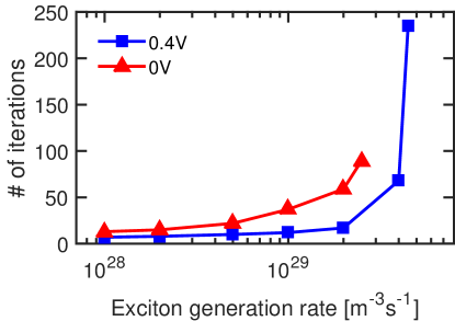
Figure 4. Number of iterations needed by the map to converge changing the value of the exciton generation rate.

7.2. Changing the zero-field charge carrier mobility

Contractivity conditions (59) depend also on the parameter $\overline{\mu}$, the maximum between the largest values of electron and hole mobilities, but, unlike the case of parameter $Q$ in Sect. 7.1, the role of $\overline{\mu}$ is far less immediate to characterize because it appears in both (59a) and (59b). Moreover, based on the mechanism of photogenerated charge transport in the acceptor and donor materials, we expect, similarly to Sect. 7.1, that a lower limit exists for the mobility parameters below which the map is not guaranteed to converge, and that the performance of the map is progressively reduced when the model parameters approach such value.

For these reasons, in the present section we carry out a numerical sensitivity analysis of $\overline{\mu}$ on the convergence of the fixed-point iteration. As both hole and electron mobilities play a role in determining the behaviour of the map and as the model we considered for them is parametrised on the mobility values at zero electric field $\mu_{n,0}$ and $\mu_{p,0}$, we decided to perform the following analyses:

• decreasing $\mu_{p,0}$ and keeping $\mu_{n,0}$ fixed at the reference value;

• decreasing $\mu_{n,0}$ and keeping $\mu_{p,0}$ fixed at the reference value;

• setting $\mu_{p,0}=\mu_{n,0}=\tilde{\mu}$ and decreasing them.

We expect the first two analyses to provide similar results as the effect of the two charge carrier densities on the model is symmetrical whereas in the third case we aim to assess whether the simultaneous change of the two mobilities results in a combined effect. Moreover, as previously done in Sect. 7.1, we consider the same two operation modes characterised by different values of the applied potential $\varphi_{C}-\varphi_{A}$ in order to determine whether this quantity has an impact on the convergence of the map while changing the mobility parameter.

In Fig. 5 we report the graphs of the number of iterations needed by the map to converge as a function of the mobility parameter, for an applied voltage equal to 0.4 V (Fig. 5) and 0 V (Fig. 5) respectively. We notice that in both cases the map performs almost similarly with the reduction of either $\mu_{p,0}$ or $\mu_{n,0}$, requiring a slightly larger number of iterations for the $p$ case at 0.4 V and for the $n$ case at 0 V. This asymmetry in the behaviour could be attributed to the marginally different reference values for the hole and electron mobilities or to a difference in the discretisation of domains $\Omega_{n}$ and $\Omega_{p}$ due to the algorithm for the generation of the anisotropic meshes. It is interesting though that when both mobilities are decreased simultaneously, the convergence to the fixed point is slower and the threshold value is considerably higher. This can be explained by the fact that by decreasing both mobilities, the charge carrier density in the donor and acceptor materials increase and, as highlighted in the discussion of Sect. 7.1, the second order term $2H\gamma np$ at the interface becomes more relevant, as both $n$ and $p$ increase.

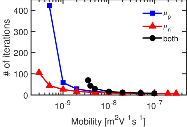
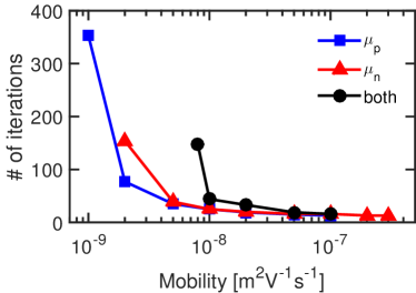
Figure 5. Number of iterations needed by the map to converge changing the value of the hole and electron mobility or both simultaneously with 0.4 V (a) or 0 V (b).

7.3. Changing the applied electric potential

Finally we want to analyse the impact of the difference in the electric potential between the electrodes $\varphi_{C}-\varphi_{A}$ on the convergence properties of the map. The obtained analytical result states that convergence to a unique fixed point is guaranteed if the applied voltage is small enough, similarly to what happens in semiconductor device modelling using the Drift-Diffusion model [25, 23], and we want to test if the map has a similar behaviour as that observed when changing $Q$ and $\mu$.

Fig. 6 shows the number of iterations needed by the map to satisfy (78) in a range of applied voltages between $-1.5$ V and $1.5$ V. Interestingly, convergence is observed for all the considered values and by increasing the applied voltage (both for negative and positive values) the convergence speed is enhanced.

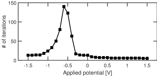
Figure 6. Number of iterations needed by the map to converge changing the value of the potential difference $\varphi_{C}-\varphi_{A}$ at the electrodes.

We already analyzed the operation mode with applied voltage equal to $0.4$ V, which can be assimilated to all the other configurations between $0$ V and $1.5$ V. The generated electric field helps charges migrate towards the electrodes, generating electric current. The charge densities in device are hence relatively small and the nonlinear terms in equations (3)-(7) are not dominant, so the map does not need to perform many steps to meet the tolerance.

Convergence has been proven more difficult in the range of values between $-0.8$ V and $-0.4$ V, with a distinct spike at $-0.6$ V. In this regime the applied voltage counteracts the potential difference determined by the displacement of the dissociated charges generating an electric field that tends to drive these latter back to the interface where they can recombine. The main consequence is that the generated output current is close to zero (open circuit regime) and also the charge carrier densities in the device are significantly larger than in the current extracting operation mode, making the nonlinear terms more important and reducing the convergence speed of the iteration map.

Furtherly decreasing the applied potential below $-0.8$ V, we observe again an improvement in the performance of the map. In these configurations, the applied electric field is strong enough to move most of the generated charge carriers back to the interface where they recombine, reducing considerably the carrier densities and hence the nonlinear effects.

7.4. Further testing of map convergence: the use of Einstein’s relation

The aim of this section is to analyse the behaviour of the iterative map in configurations where the model parameter definitions do not satisfy the assumptions of Tab. 2 made in order to prove the results of Sect. 6. A significant case is that obtained by considering the mobility parameter definition as in (74) but with no ceiling for high electric field values

(80) $$\mu_{i}\left(E\right)=\mu_{i,0}\exp\left(\dfrac{\beta_{i}\sqrt{E}}{k_{B}T}\right)$$

and assuming the Einstein-Smoluchowski relation to hold [23], i.e.

(81) $$D_{i}^{\mathrm{einstein}}\left(E\right)=\dfrac{k_{B}T}{q}\,\mu_{i}\left(E\right).$$

The study of this configuration is of particular interest as it is frequently used in the literature on the topic [28, 11, 32, 33].

Upon changing the values for the generation term $Q$ (see Fig. 7) and the zero-field mobility (see Fig. 8), the map shows a performance similar to that observed in the previous analyses. In particular, comparing with results presented in Sections 7.1 and 7.2 the number of iterations needed by the map to converge is generally higher in the configurations with no applied potential (0 V). In such configuration, the electric field in the device is close to zero, so that the diffusion coefficients are smaller than predicted by (75), that is

(82) $$D_{i}^{\mathrm{einstein}}(E\simeq 0)\simeq\dfrac{k_{B}T}{q}\mu_{i}(0)<\dfrac{k_{B}T}{q}\ \dfrac{\mu_{i}(0)+\mu_{i}(E^{\ast})}{2}=D_{i}^{\mathrm{const}}$$

as (74) is a monotonically increasing function of $E$.

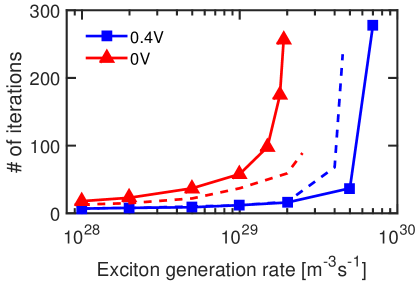
Figure 7. Number of iterations needed by the map to converge changing the value of the exciton generation rate. Results of Section 7.1 are displayed with dotted lines.

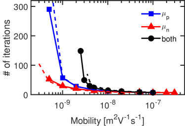
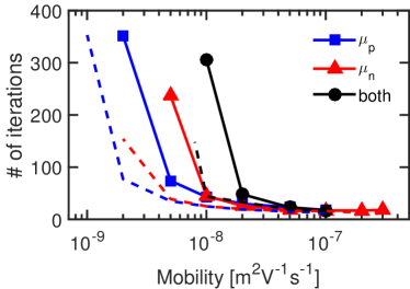
Figure 8. Number of iterations needed by the map to converge changing the value of the hole and electron mobility or both simultaneously with 0.4 V (a) or 0 V (b). Results of Section 7.2 are displayed with dotted lines.

Upon changing the value of the applied potential, we can observe an interesting behaviour of the iterative map, see Fig. 9.

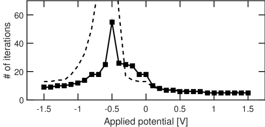
Figure 9. Number of iterations needed by the map to converge changing the value of the potential difference $\varphi_{C}-\varphi_{A}$ at the electrodes. Results of Section 7.3 are displayed with the dotted line.

The number of iterations needed for the map to converge are the same as reported in Sect. 7.3 for values of applied voltage strictly greater than 0 V. This is to be ascribed to the fact that the electric field in the device is large enough to make the drift term in the current density for electrons and holes dominant with respect to the diffusive term, in such a way that the different mathematical representations of the diffusion coefficient play no role in this branch of values of the applied external electric force. Things change in the range of values of applied potential between 0 V and -0.3 V. Indeed, in this working regime the electric field is close to zero, or small, so that relation (82) predicts $D_{i}^{\mathrm{einstein}}<D_{i}^{\mathrm{const}}$ and thus, consistently, photogenerated electrons and holes hardly diffuse from the interface region making the effect of nonlinear bimolecular recombination terms more relevant and requiring a (slightly) higher number of iterations for the map to converge. However, furtherly increasing the (negative) value of the applied voltage produces an increase of the strength of the electric field in the device, so that relation (82) does no longer hold and we have that $D_{i}^{\mathrm{einstein}}>D_{i}^{\mathrm{const}}$. As a consequence, the diffusive term in the current density helps photogenerated charges to detach from the interface region and move towards the contacts, this having the effect to reduce considerably the number of iterations for the map to converge as illustrated by the dashed line in Fig. 9. The sharp peak at -0.5 V corresponds to the open circuit conditions, and this explains the sharp increase of number of iterations: drift and diffusive current densities mutually cancel so that charges are confined at the interface and nonlinear recombination makes the convergence of the map to slow down. Then, for larger negative values of the applied voltage the behaviour of the device is again dominated by drift current densities, so that the convergence of the functional iteration becomes insensitive to the adopted model of the diffusion coefficient.

8. Conclusions and perspectives

In this article we have addressed the analytical study of a multidomain system of nonlinearly coupled PDEs, with nonlinear transmission conditions at the material interface, that represents the mathematical modeling picture of an organic solar cell. The system is constituted by a set of conservation laws for four distinct species: excitons and polarons (electrically neutral), and electrons and holes (negatively and positively charged). The analysis is conducted in the stationary regime and under assumptions on the parameters and data that make the considered problem a close representation of a realistic nanoscale device for energy photoconversion. The resulting problem is a highly nonlinearly coupled system of advection-diffusion-reaction PDEs for which existence and uniqueness of weak solutions, as well as nonnegativity of concentrations, is proved via a solution map that is a variant of the Gummel iteration commonly used in the treatment of the DD model for inorganic semiconductors. Results are established upon assuming suitable restrictions on the data and some regularity property on the mixed boundary value problem for the Poisson equation. The main analytical conclusions are numerically validated through an extensive sensitivity analysis devoted to characterizing the dependence of the convergence of the fixed-point iteration on the most relevant physical parameters of the OSC. Simulation predictions are in excellent agreement with theoretical limitations and suggest that failure to convergence may principally occur in the following three distinct conditions:

• when the exciton generation rate $Q$ becomes too large;

• when carrier mobility becomes too small;

• when the device works close to open-circuit conditions.

We believe that such conclusions may provide useful indications to improve, on the one hand, the development of efficient solution algorithms to be implemented in computational tools, and, on the other hand, the search of suitable materials in view of an optimal design of a organic solar cell of the next generation. We also believe that the functional techniques employed in the present article may be profitably adopted in the analysis of well-posedness of the multidomain nonlinear model in the time-dependent case. This aspect will be the object of our next investigation.

References

- [1] R. E. Bank, W. M. Coughran, Jr., and L. C. Cowsar. The Finite Volume Scharfetter-Gummel method for steady convection diffusion equations. Comput Vis Sci., 1(3):123–136, 1998.
- [2] J.A. Barker, C.M. Ramsdale, and N.C. Greenham. Modeling the current-voltage characteristics of bilayer polymer photovoltaic devices. Phys. Rev. B, 67:075205, 2003.
- [3] G.A. Buxton and N. Clarke. Computer simulation of polymer solar cells. Modelling Simul. Mater. Sci. Eng., 15:13–26, 2007.
- [4] M. Cogliati and M. Porro. Third generation solar cells: modeling and simulations. Master’s thesis, Politecnico di Milano, Italy, 2010.
- [5] H. Beirao da Veiga. On the semiconductor drift diffusion equations. Diff. and Int. Eqs., 9:729–744, 1996.
- [6] M. Dauge. Neumann and mixed problems on curvilinear polyhedra. Integ Equat Oper Th, 15(2):227–261, 1992.
- [7] C. de Falco and M. Culpo. bim octave-forge package. http://octave.sourceforge.net/bim/index.html.
- [8] C. de Falco and M. Culpo. msh octave-forge package. http://octave.sourceforge.net/msh/index.html.
- [9] C. de Falco, J. W. Jerome, and R. Sacco. Quantum-corrected drift-diffusion models: Solution fixed point map and finite element approximation. J. Comp. Phys., 228(5):1770 – 1789, 2009.
- [10] C. de Falco, A. L. Lacaita, E. Gatti, and R. Sacco. Quantum-corrected drift-diffusion models for transport in semiconductor devices. J. Comp. Phys., 204:533–561, 2005.
- [11] C. de Falco, M. Porro, R. Sacco, and M. Verri. Multiscale modeling and simulation of organic solar cells. Comp Meth Appl Mech Engrg, 245 - 246:102 – 116, 2012.
- [12] C. de Falco, R. Sacco, and M. Verri. Analytical and numerical study of photocurrent transients in organic polymer solar cells. Comp Meth Appl Mech Engrg, 199(25-28):1722 – 1732, 2010.
- [13] E. Gatti, S. Micheletti, and R. Sacco. A new Galerkin framework for the drift-diffusion equation in semiconductors. East-West J. Numer. Math., 6:101–136, 1998.
- [14] C. Geuzaine and J.-F. Remacle. Gmsh: A 3-d finite element mesh generator with built-in pre- and post-processing facilities. Int J Numer Meth Eng, 79(11):1309–1331, 2009.
- [15] A. Glitzky. An electronic model for solar cells including active interfaces and energy resolved defect densities. SIAM J. Math. Anal., 44:3874–3900, 2012.
- [16] K. Gröger. Initial-boundary value problems describing mobile carrier transport in semiconductor devices. Comment. Math. Univ. Carolin., 26:75–89, 1985.
- [17] K. Gröger. A -estimate for solutions to mixed boundary value problems for second order elliptic differential equations. Math. Ann., 283:679–687, 1989.
- [18] R. Haller-Dintelmann, H.-C. Kaiser, and J. Rehberg. Elliptic model problems including mixed boundary conditions and material heterogeneities. J. Math. Pures Appl., 89(1):25 – 48, 2008.
- [19] M. Hieber and J. Rehberg. Quasilinear parabolic systems with mixed boundary conditions on nonsmooth domains. SIAM J. Math. Anal., 40(1):292–305, 2008.
- [20] H. Hoppe and N. S. Sariciftci. Organic solar cells: An overview. J. Mater. Res., 19(7):1924–1945, 2004.
- [21] A. K. Hussein. Applications of nanotechnology in renewable energies - a comprehensive overview and understanding. Renew Sust Energ Rev, 42:460 – 476, 2015.
- [22] I. Hwang and N.C. Greenham. Modeling photocurrent transients in organic solar cells. Nanotechnology, 19:424012 (8pp), 2008.
- [23] J. W. Jerome. Analysis of Charge Transport. Springer, New York, 1996.
- [24] M. Lundstrom. Fundamentals of Carrier Transport, Edition 2. University Press, Cambridge, 2009.
- [25] P.A. Markowich. The Stationary Semiconductor Device Equations. Computational Microelectronics. Springer-Verlag, 1986.
- [26] P.A. Markowich, C.A. Ringhofer, and C. Schmeiser. Semiconductor Equations. Springer-Verlag, 1990.
- [27] M. Porro. Bio-polymer interfaces for optical cellular stimulation: a computational modeling approach. PhD thesis, Politecnico di Milano, Italy, 2014.
- [28] M. Porro, C. de Falco, M. Verri, G. Lanzani, and R. Sacco. Multiscale simulation of organic heterojunction light harvesting devices. COMPEL, 33(4):1107–1122, 2014.
- [29] K. Seyboth, P. Eickemeier, P. Matschoss, G. Hansen, S. Kadner, S. Schlömer, T. Zwickel, and C. von Stechow. Renewable energy sources and climate change mitigation. Special report of the intergovernmental panel on climate change. Technical report, Intergovernmental Panel on Climate Change, 2012.
- [30] S.L.M. van Mensfoort and R. Coehoorn. Effect of gaussian disorder on the voltage dependence of the current density in sandwitch-type devices based on organic semiconductors. Phys. Rev B, 78:085207, 2008.
- [31] J. Williams. Finite element simulations of excitonic solar cells and organic light emitting diodes. Master’s thesis, University of Bath, UK, 2008.
- [32] J. Williams and A.B. Walker. Two-dimensional simulations of bulk heterojunction solar cell characteristics. Nanotechnology, 19:424011, 2008.
- [33] J. H. T. Williams and A. B. Walker. Two-dimensional simulations of bulk heterojunction solar cell characteristics. Nanotechnology, 19:424011, 2008.
- [34] J. Xu and L. Zikatanov. A monotone finite element scheme for convection-diffusion equations. Math Comp, 68(228):pp. 1429–1446, 1999.
- [35] W. Ziemer. Weakly differentiable functions. Springer Verlag, New York, 1991.