Effect of electron-hole asymmetry on optical conductivity in 8-$Pmmn$ borophene

Abstract

We present a detail theoretical study of the Drude weight and optical conductivity of 8-$Pmmn$ borophene having tilted anisotropic Dirac cones. We provide exact analytical expressions of $xx$ and $yy$ components of the Drude weight as well as maximum optical conductivity. We also obtain exact analytical expressions of the minimum energy ($\epsilon_{1}$) required to trigger the optical transitions and energy ($\epsilon_{2}$) needed to attain maximum optical conductivity. We find that the Drude weight and optical conductivity are highly anisotropic as a consequence of the tilted Dirac cone. The tilted parameter can be extracted by knowing $\epsilon_{1}$ and $\epsilon_{2}$ from optical measurements. The maximum values of the components of the optical conductivity do not depend on the carrier density and the tilted parameter. The product of the maximum values of the anisotropic conductivities has the universal value $(e^{2}/4\hbar)^{2}$. The tilted anisotropic Dirac cones in 8-$Pmmn$ borophene can be realized by the optical conductivity measurement.

I introduction

Graphene is the first atomically thin two-dimensional (2D) material having isotropic Dirac cones realized in a laboratory graphene1 ; graphene2 . Since then, there have been numerous attempts to synthesize more and more new 2D materials having Dirac cones. Several quasi-2D materials possessing Dirac cones such as silicenesilicene , germanenegermanene , and MoS₂ mos2 have been synthesized experimentally and are being studied theoretically.

Recently, there has been intense research interest in synthesis of 2D crystalline boron structures, referred to as borophene. Several attempts have been made to synthesize a stable structure of borophene but only three different quasi-2D structures of borophene have been synthesized boron-syn . Various numerical experiments have predicted a large number of borophene structures with various geometries and symmetries boron0 ; boron1 . The orthorhombic 8-$Pmmn$ borophene is one of the energetically stable structures, having ground state energy lower than that of the $\alpha$-sheet structures and its analogues. The $Pmmn$ boron structures have two non-equivalent sub-lattices. The coupling and buckling between two sub-lattices and vacancy give rise to the energetic stability as well as tilted anisotropic Dirac cones boron2 . The coupling between different sub-lattices enhances the strength of the boron-boron bonds and hence gives rise to structural stability. The finite thickness is required for energetic stability of 2D boron allotropes. The orthorhombic 8-$Pmmn$ borophene possesses tilted anisotropic Dirac cones and is a zero-gap semiconductor. It can be thought of as topologically equivalent to the distorted graphene.

In the last couple of years, there have been several theoretical studies on 8-$Pmmn$ borophene. Very recently, electronic properties of 8-$Pmmn$ borophene have been studied using the first-principle calculations and have shown the Dirac cones arising from the $p_{z}$ orbitals of one of the two inequivalent sub-lattices boron2 . Zabolotskiy and Lozovik proposed a tight-binding Hamiltonian for 8-$Pmmn$ borophene and obtained a low-energy effective Hamiltonian in the continuum limit boron3 . The effective Hamiltonian successfully described all the main features of the quasi-particle spectrum as predicted in ab initio calculation. A similar Hamiltonian has been considered in Ref. hamil for studying quinoid-type graphene due to mechanical deformation and organic compound $\alpha$-(BEDT-TTF)₂I₃. The anisotropic plasmon dispersion of borophene is predicted in Ref. amit . The magnetotransport coefficients have been investigated very recently firoz .

The frequency-dependent optical conductivity is associated with the transitions from a filled band to an empty band, whereas the zero-frequency Drude weight is due to the intra-band transitions. The real part of the complex optical conductivity is connected with the absorption of the incident photon energy. Its measurement is an important tool for extracting the shape and nature of the energy bands. There are several theoretical and experimental studies on the optical conductivity in various monolayer quantum materials such as graphene graphene-op-con ; graphene-op-con1 ; op-con-exp , silicene silicene-op-con ; silicene-op-con1 ; silicene-op-con2 , MoS₂ mos2-op-con ; mos2-op-con1 , and surface states of topological insulators ti-op-con ; ti-op-con1 ; ti-op-con2 .

In this paper, we study zero-frequency Drude weight and frequency-dependent optical conductivity of 8-$Pmmn$ borophene. We find that the Drude weight and optical conductivity are highly anisotropic due to tilted Dirac cones. We obtain an analytical expression of the minimum photon energy required for triggering the optical transitions and of the photon energy at which the conductivities attain maximum value. The maximum value of the optical conductivity along the tilted and perpendicular directions are obtained, which are independent of the carrier density and tilting parameter. The spectroscopic measurement of the absorptive part of the optical conductivity can shed some light on the anisotropic but tilted Dirac cone.

This paper is organized as follows. In Sec. II, we provide basic information of 8-$Pmmn$ borophene in detail. We discuss the Drude weight and absorptive part of the optical conductivity in Sec. III. An alternate derivation of the optical conductivity using Green’s function method is provided in the Appendix. We provide a summary and conclusions in Sec. IV.

II Basic information

The massless Dirac Hamiltonian associated with the 8-$Pmmn$ borophene in the vicinity of one of the two independent Dirac points is given by boron3

$$H=v_{x}\sigma_{x}p_{x}+v_{y}\sigma_{y}p_{y}+v_{t}\sigma_{0}p_{y},$$ (1)

where $p_{\mu}$ with $\mu=x,y$ are the momentum operators, $\sigma_{\mu}$ are the $2\times 2$ Pauli matrices, and $\sigma_{0}$ is the $2\times 2$ identity matrix. The velocities are given boron3 as $v_{x}=0.86v_{F}$, $v_{y}=0.69v_{F}$, and $v_{t}=0.32v_{F}$ with $v_{F}=10^{6}$ ms^-1. The Hamiltonian associated with the second Dirac cone has the opposite sign of $v_{t}$.

The energy dispersion and the corresponding wave functions are given by

$$E_{\lambda}({\bf k})=\hbar k[v_{t}\sin{\theta_{\bf k}}+\lambda\Delta(\theta_{\bf k})]$$ (2)

and

$$\psi_{\bf k}^{\lambda}({\bf r})=\frac{e^{i\textbf{k}\cdot\textbf{r}}}{\sqrt{2}}\begin{pmatrix}1\\ \lambda e^{i\phi}\end{pmatrix},$$ (3)

where $\lambda=\pm$ denotes the conduction and valence bands, respectively, $\theta_{\bf k}=\tan^{-1}(k_{y}/k_{x})$, $\Delta(\theta_{\bf k})=\sqrt{v_{x}^{2}\cos^{2}{\theta_{\bf k}}+v_{y}^{2}\sin^{2}{\theta_{\bf k}}}$ describes anisotropy of the spectrum and $\phi=\tan^{-1}(v_{y}k_{y}/v_{x}k_{x})$. The energy difference between the conduction and valence bands at a given ${\bf k}$ is $E_{g}({\bf k})=E_{+}({\bf k})-E_{-}({\bf k})=2\hbar k\Delta(\theta_{\bf k})$. Note that the first term in the energy spectrum tilts the Dirac cone and breaks the electron-hole symmetry $E_{\lambda}({\bf k})=-E_{-\lambda}({\bf k})$, even for the isotropic case $v_{x}=v_{y}$. The tilted Dirac cones are depicted in Fig. 1.

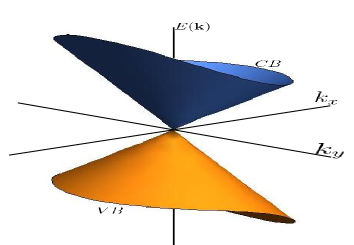
Figure 1: Plots of $E$-${\bf k}$ dispersion displaying the tilted anisotropic Dirac cones.

The Berry connection of 8-$Pmmn$ borophene is given by

$${\bf A}_{\lambda}({\bf k})=-\frac{v_{x}v_{y}}{2\Delta^{2}(\theta_{\bf k})}\,\frac{\hat{\theta}_{\bf k}}{k},$$ (4)

where $\hat{\theta}_{\bf k}=-\sin\theta_{\bf k}\,\hat{x}+\cos\theta_{\bf k}\,\hat{y}$ is the unit polar angle. The corresponding Berry phase is $\gamma_{\lambda}=\oint{\bf A}_{\lambda}({\bf k})\cdot d{\bf k}=\pi$, exactly the same as in the monolayer graphene case.

The chirality operator can be defined as

$${\hat{\Lambda}}=\frac{v_{x}\cos\theta_{\bf k}\,\sigma_{x}+v_{y}\sin\theta_{\bf k}\,\sigma_{y}}{\Delta(\theta_{\bf k})}.$$ (5)

It can be easily checked that the chirality operator ${\hat{\Lambda}}$ commutes with the Hamiltonian $H$ even in the presence of the tilted Dirac cone and the eigenfunctions $\psi_{\bf k}^{\lambda}({\bf r})$ are also eigenfunctions of the chirality operator with the eigenvalues $\lambda=\pm 1$, respectively.

The role of the Berry phase $\gamma_{\lambda}=\pi$ and of the chiral symmetry preservation must be reflected in the scattering process. This can be easily understood by analyzing the angular scattering probability for the borophene. This is given by the squared moduli of the overlap matrix element between the initial spinor ($\chi_{\lambda}(\theta_{\bf k})$) and the final spinor ($\chi_{\lambda}(\theta_{\bf k}^{\prime})$) with $|{\bf k}|=|{\bf k}^{\prime}|$. The angular scattering probability is then

$$|f(\theta_{\bf k},\theta_{{\bf k}^{\prime}})|^{2} = |\langle\chi_{\lambda}(\theta_{\bf k})|\chi_{\lambda}(\theta_{{\bf k}^{\prime})}\rangle|^{2}$$

$$= \frac{1}{2}\Big{[}1+\frac{v_{x}^{2}\cos\theta_{\bf k}\cos\theta_{{\bf k}^{\prime}}+v_{y}^{2}\sin\theta_{\bf k}\sin\theta_{{\bf k}^{\prime}}}{\Delta(\theta_{\bf k})\Delta(\theta_{{\bf k}^{\prime}})}\Big{]}.$$

It is to be noted that the wave functions do not depend on the tilt parameter $v_{t}$. Hence the Berry connection and $|f(\theta_{\bf k},\theta_{{\bf k}^{\prime}})|^{2}$ are also independent of the tilt parameter. It also shows that $|f(\theta_{\bf k},\theta_{{\bf k}^{\prime}})|^{2}$ is independent of the bands and vanishes exactly when $\theta_{{\bf k}^{\prime}}-\theta_{\bf k}=\pi$. It implies that the backscattering is completely absent, similar to the graphene case. The absence of backscattering survives even for tilted anisotropic energy spectrum. This is due to the conservation of the chirality and/or the $\mp\pi$ Berry phase.

The density of states is given by

$$D(E) = g_{s}g_{v}\int\frac{d^{2}k}{(2\pi)^{2}}\delta(E-E_{\lambda}({\bf k}))$$ (6)

$$= N_{0}\frac{|E|}{\pi^{2}\hbar^{2}v_{F}^{2}},$$

where the spin degeneracy $g_{s}=2$ and the “valley degeneracy” $g_{v}=2$ lozovik1 . Also, the constant $N_{0}$ is given by

$$N_{0}=\int_{0}^{2\pi}\frac{v_{F}^{2}\;d\theta_{\bf k}}{[v_{t}\sin\theta_{\bf k}+\lambda\Delta(\theta_{\bf k})]^{2}}=15.2263.$$

For a given carrier density $n_{c}$, the Fermi energy is $E_{F}=\hbar\tilde{v}_{F}\sqrt{\pi n_{c}}$ with $\tilde{v}_{F}=\sqrt{2\pi/N_{0}}v_{F}$ and the associated anisotropic Fermi wave vectors are obtained as

$$k_{F}^{\lambda}(\theta_{\bf k}) = \frac{E_{F}}{\hbar|v_{t}\sin\theta_{\bf k}+\lambda\Delta(\theta_{\bf k})|}.$$ (7)

The components of the velocity operator along the $x$- and $y$-directions are $\hat{v}_{x}=v_{x}\sigma_{x}$ and $\hat{v}_{y}=v_{t}\sigma_{0}+v_{y}\sigma_{y}$. The expectation values of these operators are given by $\langle\hat{v}_{x}\rangle_{\lambda}=[v_{x}^{2}/\Delta(\theta_{\bf k})]\cos{\theta_{\bf k}}$ and $\langle\hat{v}_{y}\rangle_{\lambda}=v_{t}+[v_{y}^{2}/\Delta(\theta_{\bf k})]\sin{\theta_{\bf k}}$, respectively.

III optical conductivity

We consider $n$-doped 8-$Pmmn$ borophene subjected to zero-momentum electric field ${\bf E}\sim\hat{\boldsymbol{\mu}}E_{0}e^{i\omega t}$ with oscillation frequency $\omega$ ($\hat{\boldsymbol{\mu}}=\hat{\bf x},\hat{\bf y}$). The complex charge optical conductivity tensor is given by $\Sigma_{\mu\nu}(\omega)=\delta_{\mu\nu}\sigma_{D}(\omega)+\sigma_{\mu\nu}(\omega)$, where $\mu,\nu=x,y$, $\sigma_{D}(\omega)=\sigma_{d}/(1-i\omega\tau)$ is the dynamic Drude conductivity due to the intra-band transitions, with $\sigma_{d}$ being the static Drude conductivity and $\sigma_{\mu\nu}(\omega)$ being the complex optical conductivity due to transitions between valence and conduction bands. It should be mentioned here that Re $\sigma_{D}$ and Re $\sigma_{\mu\nu}$ correspond to the absorption of the photon energy.

Drude weight: The Drude weight at vanishingly low-temperature is given by mermin

$$D_{\mu\nu}=\frac{g_{s}g_{v}e^{2}}{4\pi}\int d^{2}k\,\langle\hat{v}_{\mu}\rangle\langle\hat{v}_{\nu}\rangle\delta(E({\bf k})-E_{F}),$$ (8)

On further simplification, we obtain

$$D_{\mu\nu}=\frac{e^{2}}{\hbar}\frac{E_{F}}{\pi\hbar}\delta_{\mu\nu}(\delta_{\mu x}N_{1}+\delta_{\nu y}N_{2}),$$ (9)

where $N_{1}=4.686$ and $N_{2}=2.673$. In this case, the Drude weight is anisotropic, unlike the monolayer graphene case where the Drude weight $D_{w}^{G}=(v_{F}e^{2}/\hbar)\sqrt{\pi n_{c}}$ is isotropic.

Optical Conductivity: Within the linear response theory, the Kubo formula for the optical conductivity tensor $\sigma_{\mu\nu}(\omega)$ is given by

$$\sigma_{\mu\nu}(\omega) = \frac{1}{\hbar(\omega+i\eta)}\int_{0}^{\infty}dte^{i(\omega+i\eta)t}\langle[\hat{j}_{\mu}(t),\hat{j}_{\nu}(0)]\rangle,$$

where $\langle[\hat{j}_{\mu}(t),\hat{j}_{\nu}(0)]\rangle=\sum_{m,n}[f(E_{n})-f(E_{m})]e^{i(E_{n}-E_{m})t/\hbar}j_{\mu}^{nm}j_{\nu}^{mn}$, $\hat{j}_{\mu}=e\hat{v}_{\mu}$ is the charge current density with $\mu=x,y$, $f(E)$ is the Fermi-Dirac distribution function and $\eta\rightarrow 0^{+}$. Here $E_{n}$ and $E_{m}$ are the discrete energy levels of the system. So changing the sum into integration over momentum space, the real part of the charge optical conductivity is given by

$${\rm Re\;\sigma_{\mu\nu}(\omega)} = \frac{e^{2}}{4\pi\omega}\int d^{2}k[f(E_{-}(\textbf{k}))-f(E_{+}(\textbf{k}))]$$ (10)

$$v_{\mu}^{-+}({\bf k})v_{\nu}^{+-}({\bf k})\delta(E_{g}({\bf k})-\hbar\omega).$$

The final expression of the real part of the optical conductivity tensor is given by

$${\rm Re\;\sigma_{\mu\nu}}(\omega)=\frac{e^{2}}{4\pi\hbar}\int_{0}^{2\pi}d\theta_{\bf k}\frac{v_{x}^{2}v_{y}^{2}}{\Delta^{4}(\theta_{\bf k})}[f(E_{-})-f(E_{+})][(\delta_{\mu x}\sin^{2}{\theta_{\bf k}}+\delta_{\nu y}\cos^{2}{\theta_{\bf k}})\delta_{\mu\nu}-(1-\delta_{\mu\nu})\sin{\theta_{\bf k}}\cos{\theta_{\bf k}}],$$ (11)

where $E_{\pm}(k_{\omega}(\theta_{\bf k}),\theta_{\bf k})\equiv E_{\pm}$ with $k_{\omega}(\theta_{\bf k})=\omega/[2\Delta(\theta_{\bf k})]$.

First of all, we find that the real part of the off-diagonal optical conductivity ${\rm Re}\;\sigma_{xy}(\omega)$ vanishes exactly. For monolayer graphene ($v_{t}=0$ and $v_{x}=v_{y}=v_{F}$), Eq. (11) gives featureless isotropic optical conductivity which has a step-like shape with a step height $\sigma_{0}=e^{2}/4\hbar$ at $\hbar\omega=2E_{F}^{0}=2\hbar v_{F}\sqrt{\pi n_{c}}$. Whereas tilted Dirac cones in borophene provide a distinct anisotropic optical conductivity which can be seen in the subsequent discussion.

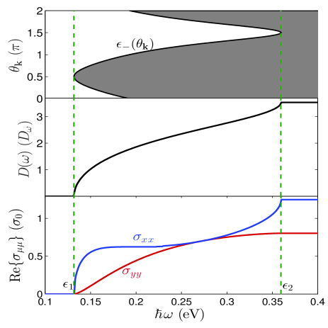
Figure 2: Top panel: Plots of $\epsilon_{-}(\theta_{\bf k})$ versus $\theta_{\bf k}$. Middle panel: plots of the joint density of states versus photon energy $\hbar\omega$. Bottom panel: Plots of the optical conductivities ${\rm Re}\;\sigma_{xx}(\omega)$ and ${\rm Re}\;\sigma_{yy}(\omega)$ in units of $\sigma_{0}=e^{2}/4\hbar$ versus photon energy $\hbar\omega$.

We analyze the real part of the optical conductivity by solving Eq. (11) numerically for electron density $n_{c}=1.0\times 10^{16}$ m^-2 at $T=0$. The plots of ${\rm Re}\;\sigma_{xx}(\omega)$ and ${\rm Re}\;\sigma_{yy}(\omega)$ as a function of photon energy $\hbar\omega$ are shown in the lower panel of Fig. 2. It exhibits anisotropic nature of the optical conductivity. We plot $\epsilon_{-}(\theta_{\bf k})=2\hbar k_{F}^{-}(\theta_{\bf k})\Delta(\theta_{\bf k})$ in the top panel of Fig. 2. The shaded region in the top panel contributes to the optical conductivity. The optical transition from the valence band to the conduction band takes place when the photon energy satisfies the inequality $\hbar\omega\geq\epsilon_{-}(\theta_{\bf k})$. The optical transition begins at $\hbar\omega=0.113$ eV, which corresponds to $\epsilon_{1}=\epsilon_{-}(\pi/2)=2E_{F}\frac{v_{y}}{v_{y}+v_{t}}<2E_{F}$. Moreover, the optical conductivities attain a maximum value when $\hbar\omega=0.359$ eV, which corresponds to $\epsilon_{2}=\epsilon_{-}(3\pi/2)=2E_{F}\frac{v_{y}}{v_{y}-v_{t}}>2E_{F}$. Note that the two energy scales $\epsilon_{1}$ and $\epsilon_{2}$ depend on the carrier density, tilted parameter $v_{t}$ and the velocity $v_{y}$ along the tilted direction. We have checked numerically that ${\rm Re}\;\sigma_{xx}(\omega)={\rm Re}\;\sigma_{yy}(\omega)$ when $\hbar\omega\simeq 2E_{F}$. By knowing the energies $\epsilon_{1}$ and $\epsilon_{2}$ from an experimental measurement, one can extract the tilted parameter $v_{t}$ using the relation

$$v_{t}=v_{y}E_{F}\Big{[}\frac{1}{\epsilon_{1}}-\frac{1}{\epsilon_{2}}\Big{]}.$$ (12)

Analyzing the lower panel of Fig. 2, the maximum attainable absorptive part of the conductivity along the tilted direction is $\sigma_{yy}^{\rm max}=\sigma_{0}(v_{y}/v_{x})<\sigma_{0}$ and its orthogonal axis is $\sigma_{xx}^{\rm max}=\sigma_{0}(v_{x}/v_{y})>\sigma_{0}$. It is interesting to note that $\sigma_{xx}^{\rm max}$ and $\sigma_{yy}^{\rm max}$ do not depend on the carrier density as well as the tilted parameter $v_{t}$. Moreover, $\sigma_{xx}^{\rm max}>\sigma_{yy}^{\rm max}$ and the product of these two conductivities $\sigma_{xx}^{\rm max}\cdot\sigma_{yy}^{\rm max}=\Big{(}\frac{e^{2}}{4\hbar}\Big{)}^{2}$ is universal.

To confirm the results of the optical conductivity, we analyze the joint density of states which is given by

$$D(\omega)=\int_{0}^{2\pi}\frac{dC[f(E_{-}(k_{\omega},\theta_{\bf k}))-f(E_{+}(k_{\omega},\theta_{\bf k}))]}{4\pi^{2}|\partial_{k}E_{g}({\bf k})|_{E_{g}=\hbar\omega}},$$ (13)

where $C$ is the line element along the contour. In the middle panel of Fig. 2, we show the joint density of states versus the photon energy $\hbar\omega$. One can easily see that that the van Hove singular points are at $\theta_{\bf k}=\theta_{s}=\pi/2,3\pi/2$. The region of zero optical conductivity is nicely captured by the joint density of states.

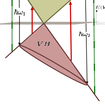
Figure 3: Sketch of the allowed (dotted-dash-green) and forbidden (solid-red) inter-band transitions for $n$-doped borophene.

The absorptive part of the optical conductivity arises due to the transitions from the valence band to the conduction band for a given momentum as demonstrated in Fig. 3. The green (dashed) and red (solid) arrows indicate the allowed and forbidden transitions, respectively. One can easily see from this sketch that there are no allowed transitions for the photon energy $\hbar\omega<\epsilon_{1}$ as a result of the Pauli blocking. One can also notice that the transitions are allowed even for $\hbar\omega>\epsilon_{2}$.

IV Summary and conclusions

We have presented detailed theoretical studies of the Drude weight and optical conductivity of the 8-$Pmmn$ borophene. The exact analytical expressions of the Drude weight, components of the optical conductivity and the onset energy needed for initiating the optical transitions are provided. We also obtain an analytical expression for the photon energy required to attain maximum optical conductivity. We find that the Drude weight and the absorptive parts of the optical conductivity are strongly anisotropic as a result of the tilted Dirac cones. The tilted parameter $v_{t}$ and the velocity components ($v_{x},v_{y}$) can be extracted from experimental measurements. We have shown that the product of the maximum values of the anisotropic conductivities is always universal.

V Acknowledgements

We would like to thank Arijit Kundu and SK Firoz Islam for useful discussion.

Appendix A Alternative derivation of the optical conductivity

We provide an alternative derivation of the optical conductivity using Green’s function method.. The Kubo formula for the optical conductivity is given by

$$\sigma_{\mu\nu}(\omega)=i\frac{e^{2}}{\omega}\frac{1}{(2\pi)^{2}}\int d^{2}k$$

$$\times T\sum_{n}\textrm{Tr}\langle\hat{v}_{\mu}\hat{G}({\bf k},\omega_{n})\hat{v}_{\nu}\hat{G}({\bf k},\omega_{n}+\omega_{l})\rangle_{i\omega_{n}\rightarrow\omega+i\delta}.$$ (14)

Here, $T$ is the temperature and $n$ and $l$ are integers, where $\omega_{l}=(2l+1)\pi T$ and $\omega_{n}=2n\pi T$ are the fermionic and bosonic Matsubara frequencies, respectively.

The Green’s function of the Hamiltonian in Eq. (1) is given by

$$\hat{G}({\bf k},\omega) = \sum_{\lambda}\Big{[}\sigma_{0}-\frac{\lambda}{\Delta(\theta_{\bf k})}\big{(}v_{x}\cos\theta_{\bf k}\;\sigma_{x}+v_{y}\sin\theta_{\bf k}\;\sigma_{y}\big{)}\Big{]}$$ (15)

$$\times G_{\lambda}({\bf k},\omega),$$

where $G_{\lambda}({\bf k},\omega)=[i\hbar\omega+\mu-E_{\lambda}({\bf k})]^{-1}$. Using this Green’s function, the following trace is obtained as

$$\textrm{Tr}\langle\hat{v}_{x}\hat{G}({\bf k},\omega_{n})\hat{v}_{x}\hat{G}({\bf k},\omega_{n}+\omega_{l})\rangle=\sum_{\lambda,\lambda^{\prime}}\Big{[}\frac{v_{x}^{2}}{2}(1-\lambda\lambda^{\prime})+\lambda\lambda^{\prime}\frac{v_{x}^{4}\cos^{2}\theta_{\bf k}}{\Delta^{2}(\theta_{\bf k})}\Big{]}G_{\lambda}({\bf k},\omega_{l})G_{\lambda^{\prime}}({\bf k},\omega_{l}+\omega_{n}).$$ (16)

Using the well-known identity

$$T\sum_{s}\bigg{[}\frac{1}{i\hbar\omega_{n}+\mu-E_{\lambda}}\cdot\frac{1}{i\hbar(\omega_{l}+\omega_{n})+\mu-E_{\lambda^{\prime}}}\bigg{]}=\begin{cases}\frac{f(E_{\lambda})-f(E_{\lambda^{\prime}})}{i\hbar\omega_{n}-E_{\lambda^{\prime}}+E_{\lambda}},&\text{if }\lambda\neq\lambda^{\prime}\\ 0,&\text{otherwise.}\end{cases}$$ (17)

One can further simply the above equation as

$$T\sum_{n}\textrm{Tr}\langle\hat{v}_{x}\hat{G}({\bf k},\omega_{n})\hat{v}_{x}\hat{G}({\bf k},\omega_{l}+\omega_{n})\rangle=\frac{v_{x}^{2}v_{y}^{2}\sin^{2}\theta_{\bf k}}{\Delta^{2}(\theta_{\bf k})}\Big{[}\frac{f[E_{-}({\bf k})]-f[E_{+}({\bf k})]}{i\hbar\omega_{n}-E_{+}({\bf k})+E_{-}({\bf k})}+\frac{f[E_{+}({\bf k})]-f[E_{-}({\bf k})]}{i\hbar\omega_{n}-E_{-}({\bf k})+E_{+}({\bf k})}\Big{]}.$$ (18)

It can be seen that the second term turns out to be zero as a result of the conservation of energy. Using the result of Eq. (18) into Eq. (A), we have

$$\sigma_{xx}(\omega)=\frac{ie^{2}}{(2\pi)^{2}\omega}\int_{0}^{\infty}\int_{0}^{2\pi}dkd\theta_{\bf k}\frac{v_{x}^{2}v_{y}^{2}\;k\sin^{2}\theta_{\bf k}}{\Delta^{2}(\theta_{\bf k})}\frac{f[E_{-}({\bf k})]-f[E_{+}({\bf k})]}{i\hbar\omega_{n}-E_{+}({\bf k})+E_{-}({\bf k})}\Big{|}_{i\omega_{n}\rightarrow\omega+i\delta}.$$ (19)

The real part of the optical conductivity is given by

$${\rm Re}\;\sigma_{xx}(\omega)=\frac{e^{2}}{4\pi}\int dkd\theta_{\bf k}\frac{v_{x}^{2}v_{y}^{2}\;k\sin^{2}\theta_{\bf k}}{\Delta^{2}(\theta_{\bf k})}\Big{[}f(E_{-}({\bf k}))-f(E_{+}({\bf k}))\Big{]}\delta(\hbar\omega-2\hbar k\Delta(\theta_{\bf k})).$$ (20)

The above Eq. (20) can be further simplified to

$${\rm Re}\;\sigma_{xx}(\omega)=\frac{e^{2}}{16\pi}\int_{0}^{2\pi}d\theta_{\bf k}\frac{v_{x}^{2}v_{y}^{2}\sin^{2}\theta_{\bf k}}{\Delta^{4}(\theta_{\bf k})}\Big{[}f(E_{-}({k_{\omega}(\theta_{\bf k})}))-f(E_{+}(k_{\omega}(\theta_{\bf k})))\Big{]}$$ (21)

where $k_{\omega}(\theta_{\bf k})=\omega/2\Delta(\theta_{\bf k})$.

Similarly, the $yy$ and $yx$ components of the optical conductivity can be obtained as

$${\rm Re}\;\sigma_{yy}(\omega) = -\frac{e^{2}}{16\pi}\int_{0}^{2\pi}d\theta_{\bf k}\frac{v_{x}^{2}v_{y}^{2}\cos^{2}\theta_{\bf k}}{\Delta^{4}(\theta_{\bf k})}\Big{[}f(E_{+}(k_{\omega}(\theta_{\bf k})))-f(E_{-}(k_{\omega}(\theta_{\bf k})))\Big{]},$$ (22)

$${\rm Re}\;\sigma_{yx}(\omega) = \frac{e^{2}}{16\pi}\int_{0}^{2\pi}d\theta_{\bf k}\frac{v_{x}^{2}v_{y}^{2}\sin\theta_{\bf k}\cos\theta_{\bf k}}{\Delta^{4}(\theta_{\bf k})}\Big{[}f(E_{+}(k_{\omega}(\theta_{\bf k})))-f(E_{-}(k_{\omega}(\theta_{\bf k})))\Big{]}.$$ (23)

Equations (21), (22) and (23) can be written in a compact form as given in Eq. (11).

References

• (1) A. K. Geim and K. S. Novoselov, Nature Materials 6, 183-191 (2007).
• (2) D. Pesin and A. H. MacDonald, Nature Materials 11, 409 (2012).
• (3) B. Feng, H. Li, C. Liu, T. Shao, P. Cheng, Y. Yao, S. Meng, L. Chen, and K. Wu, ACS Nano, 7 (10), pp 9049–9054 (2013).
• (4) R. Quhe, Y. Yuan, J. Zheng, Y. Wang, Z. Ni, J. Shi, D. Yu, J. Yang, and J. Lu, Scientific Reports 4, 5476 (2014).
• (5) K. F. Mak, C. Lee, J. Hone, J. Shan, and T. F. Heinz, Phys. Rev. Lett. 105, 136805 (2010).
• (6) A. J. Mannix, X. F. Zhou, B. Kiraly, J. D. Wood, D. Alducin, B. D. Myers, X. Liu, B. L. Fisher, U. Santiago, J. R. Guest, M. J. Yacaman, A. Ponce, A. R. Oganov, M. C. Hersam, and N. P. Guisinger, Science 350, 1513 (2015).
• (7) L. Xu, A. Du, and L. Kou, Phys. Chem. Chem. Phys. 18, 27284 (2016).
• (8) X. F. Zhou, X. Dong, A. R. Oganov, Q. Zhu, Y. Tian, and H. T. Wang, Phys. Rev. Lett 112, 085502 (2014).
• (9) A. L. Bezanilla and P. B. Littlewood, Phys. Rev. B 93, 241405 (2016).
• (10) A. D. Zabolotskiy and Yu. E. Lozovik, Phys. Rev. B 94, 165403 (2016).
• (11) M. O. Goerbig, J.-N. Fuchs, G. Montambaux, and F. Piechon, Phys. Rev. B 78, 045415 (2008).
• (12) K. Sadhukhan and A. Agarwal, Phys. Rev. B 96, 035410 (2017).
• (13) SK F. Islam and A. Jayannavar, arXiv: 1707.05578
• (14) V. P. Gusynin, S. G. Sarapov, and J. P. Carbotte, Phys. Rev. B 75, 165407 (2007).
• (15) T. Stauber, N. M. R. Peres, and A. K. Geim, Phys. Rev. B, 78, 085432 (2008).
• (16) K. F. Mak, M. Y. Sfeir, Y. Wu, C. H. Lui, J. A. Misewich, and T. F. Heinz, Phys. Rev. Lett. 101, 196405 (2008).
• (17) L. Stille, C. J. Tabert, and E. J. Nicol, Phys. Rev. B 86, 195405 (2012).
• (18) L. Mathes, P. Gori, O. Pulci, and F. Bechstedt, Phys. Rev. B 87, 035438 (2013).
• (19) C. J. Tabert and E. J. Nicol, Phys. Rev. B 87, 235426 (2013).
• (20) Z. Li and J. P. Carbotte, Phys. Rev. B 86, 205425 (2012).
• (21) I. Milosevic, B. Nikolic, E. Dobardzic, M. Damnjanovic, I. Popov, and G. Seifert, Phys. Rev. B 76, 234414 (2007).
• (22) P. D. Pietro, F. M. Vitucci, D. Nicoletti, L. Baldassarre, P. Calvani, R. Cava, Y. S. Hor, U. Schade, and S. Lupi, Phys. Rev. B 86, 045439 (2012).
• (23) Z. Li and J. P. Carbotte, Phys. Rev. B 87, 155416 (2013).
• (24) X. Xiao and W. Wen, Phys. Rev. B 88, 045442 (2013).
• (25) Y. E. Lozovik (private communication, September 2016).
• (26) N. W. Ashcroft and N. D. Mermin, Solid State Physics, (Harcourt College Publishes-2001).