Inference from Randomized Transmissions by Many Backscatter Sensors

Abstract

Attaining the vision of Smart Cities requires the deployment of an enormous number of sensors for monitoring various conditions of the environment ranging from air quality to traffic. Backscatter sensors have emerged to be a promising solution for two reasons. First, transmissions by backscattering allow sensors to be powered wirelessly by radio-frequency (RF) waves, overcoming the difficulty in battery recharging for billions of sensors. Second, the simple backscatter hardware leads to low-cost sensors suitable for large-scale deployment. On the other hand, backscatter sensors with limited signal-processing capabilities are unable to support conventional algorithms for multiple access and channel training. Thus, the key challenge in designing backscatter sensor networks is to enable readers to accurately detect sensing values given simple ALOHA random access, primitive transmission schemes, and no knowledge of channel states and statistics. We tackle this challenge by proposing the novel framework of backscatter sensing (BackSense) featuring random encoding at backscatter sensors and statistical inference at readers. Specifically, assuming the widely used on/off keying for backscatter transmissions, the practical random-encoding scheme causes the on/off transmission of a sensor to be randomized and follow a distribution parameterized by the sensing values. Facilitated by the scheme, statistical inference algorithms are designed to enable a reader to infer sensing values from randomized transmissions by multiple backscatter sensors. The specific design procedure involves the construction of Bayesian networks, namely deriving conditional distributions for relating unknown parameters and variables (including sensing values, noise power, sensing measurements, number of active sensors) to signals observed by the reader. Then based on the Bayesian networks and the well-known expectation-maximization (EM) principle, inference algorithms are derived to recover sensing values. Simulation of the BackSense system demonstrates high accuracy in reader inference despite the mentioned limitations of backscatter sensors, which grows with increasing numbers of received symbols and reader antennas.

I Introduction

Realizing the visions of Internet-of-Things (IoT) and Smart Cities will require the deployment of billions of wireless IoT sensors in our society for automating a wide range of applications such as health care, smart homes, pollution and traffic monitoring, and industrial control. Backscatter transmission has emerged to be a promising solution for tackling some key challenges on deploying large-scale sensor networks. The main feature of a backscatter radio is to transmit by backscattering and modulating an incident radio-frequency (RF) wave [1]. This allows backscatter sensors to be powered wirelessly by a reader, overcoming the difficulty of battery recharging for a massive number of sensors. Furthermore, requiring no oscillators and RF components, backscatter sensors can be manufactured to have a small form factor and low cost. Thereby, they are suitable for large-scale deployment. Last, with recent advancements in multi-antenna beamforming and low-power electronics, the ranges for backscatter links have been increased from several meters in the classic RFID applications to tens of meters in state-of-the-art systems [2, 3]. This makes it possible to collect measurement data from backscatter sensors using versatile mobile readers mounted on vehicles and unmanned aerial vehicles (UAVs) (see Fig. 1). Motivated by the potential of backscatter sensor networks, this work presents a novel design framework, called randomized backscatter sensing (BackSense), for sensing-data uploading and detection based on random access and machine learning. To be specific, to resolve transmission collisions, statistical-inference algorithms are designed for readers to directly infer sensing values from collided signals by exploiting their spatial correlation and partial information of their distributions. The algorithms build on a proposed scheme of randomized on/off transmissions targeting backscatter sensors.

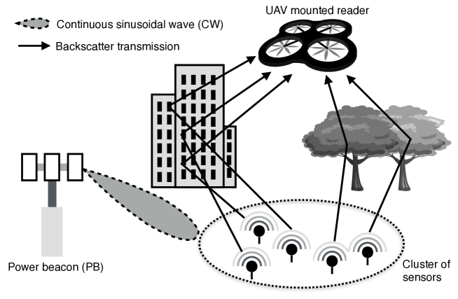
Figure 1: A BackSense system comprising a cluster of sensors deployed at a remote or hazardous location, a PB wirelessly powering the sensors, and a UAV mounted reader for collecting sensing data.

I-A Backscatter Communications and Networking

Backscatter communications are expected to play a key role in next-generation sensor systems e.g., IoT and Smart Cities. These applications motivate growing research on developing advanced techniques for backscatter communications that are more complex than those for the traditional RFID applications [1, 4, 5, 6, 7, 8]. The modulation and space-time coding schemes were designed in [1] for enhancing the rate and reliability of backscatter communication links. Traditionally, a reader transmits a single sinusoidal wave for powering a backscatter tag but such a design is sub-optimal in terms of energy harvesting efficiency. Instead, a waveform design superimposing multiple sinusoidal waves was proposed in [4] for enhancing the efficiency, via optimization based on the harvester-response function. For backscatter tags with low-complexity, non-coherent detection schemes are preferred due to the simple transmitter architecture. Specific schemes based on on/off keying or frequency-shift keying were proposed in [5] and [6], respectively. The channel-utilization efficiency for backscatter communications tends to be low as the primitive backscatter architecture is incapable of supporting sophisticated transmission designs such as high-order modulation or spatial multiplexing. An attempt was made in [7] on improving the efficiency by designing full-duplex backscatter communication networks. In this design, full-duplexing is realized by double (coherent and non-coherent) modulating backscattered signals and using time-hopping spread spectrum to mitigate interference. Last, to extend the ranges as well as simultaneoully power a large number of sensors, a novel architecture for backscatter communication networks was recently proposed in [8] where tags are powered by distributed power beacons (PBs) instead of readers. Then the tradeoff between network coverage and PB density was studied therein using a stochastic-geometric network model.

A key design issue for backscatter sensor networks is multiple access by sensors. The natural design approach is to adopt classic multiple-access schemes including random access [9, 10], time division multiple access (TDMA) [11, 12], space-division multiple access (SDMA) [13, 14], and code division multiple access (CDMA) [15, 16]. As mentioned, for large-scale sensors networks, these schemes have the drawbacks of excessive network overhead due to protocols and algorithms for orthogonalizing transmissions as well as long latency and low spectrum-utilization efficiency. Moreover, the required signal processing (e.g., FFT, channel estimation and feedback) are impractical for backscatter sensors with a primitive hardware architecture. On the other hand, ALOHA-type random access does not have the above drawbacks but suffers from performance degradation caused by transmission collisions. A novel approach for resolving collisions is proposed in [16]. Specifically, assuming sparse random access by backscatter tags, collided signals are treated as a sparse code and recovered using the techniques of compressive sensing and rateless coding. The design is effective only in the scenario of dense but mostly inactive sensors and thus cannot support the deployment of dense sensor networks with many active sensors.

I-B Machine Learning for Wireless Sensor Networks

Machine learning provides a rich set of techniques for learning and prediction of data. Recent breakthroughs in the field especially the area of artificial intelligence motivated researchers to apply relevant techniques for bringing intelligence to communication systems and networks (e.g., UAV assisted networking [17] and molecular communication [18]). In particular, a thrust of the research focuses on applying machine-learning techniques to streamline various operations of sensors networks such as routing [19], abnormality detection [20], positioning and network topology discovery [21], and sensing-data compression and feature extraction [22].

The existing research most relevant to the current work is the application of statistical-learning techniques to detection of sensing values from signals transmitted by wireless sensors based on random access [23, 24, 25, 26, 27]. In [23, 24], the sensors are designed such that their noisy measurements received by the reader provide sufficient statistics of the measured environmental parameter, thereby allowing it to be inferred using the classic maximum-likelihood algorithm. This requires each sensor to estimate and inverse its channel to the reader and furthermore map the noisy measurement to a pre-determined set of orthogonal waveforms. Such operations, however, are too complex for a backscatter sensor that usually supports only primitive signal processing and modulates signals using the simple on/off keying. In a series of other research, advanced machine-learning techniques were applied to enhance the performance of the carrier-sensing multiple access (CSMA) scheme [25, 26, 27]. In [25], cognitive transmitting sensors rely on statistical inference to infer the channel status (idle or busy) at the receiver based on local measurements. Such information allows the sensors to intelligently switch between active and sleep modes to avoid collision and reduce energy consumption. A different kind of cognitive sensor is designed in [26] based on reinforcement learning to have the capability of adapting its duty cycle according to the traffic load and channel state, thereby reducing its energy consumption as well as enhancing network throughput. Another technique, namely neural network, is applied in [27] to learn the optimal scheduling policy that minimizes a schedule cycle such that all sensors can be scheduled within each cycle without any collision. The existing designs of cognitive transmitters are impractical for backscatter sensors again due to their low complexity and limited signal-processing capability. The more practical approach, especially for large-scale sensor networks, should be one reducing sensor complexity and compensating for it by centralized machine learning at readers or in the cloud.

I-C Contributions and Organization

Based on this approach, we design techniques for efficient implementation of backscatter sensor networks. Specifically, adopting the network architecture proposed in [8], we consider a system illustrated in Fig. 1 where a cluster of backscatter sensors are powered wirelessly by a PB for transmission to a mobile reader (also called an information collector) mounted on e.g., a UAV. The BackSense framework for designing such a system satisfies several practical constraints. First, the transmission of each sensor is based on on/off keying. Second, multiple access by sensors is based on the simple ALOHA-type random access (without carrier sensing and scheduling). Last, both sensors and reader have neither channel state information (CSI) nor parameters of channel distribution. The only knowledge the reader has about the channels is their distribution type. Under these constraints, the BackSense framework is designed for efficient sensing-data uploading and accurate detection. To the best of the authors’ knowledge, this current work represents the first attempt on applying machine learning to the design of backscatter-sensor systems. The resultant BackSense framework comprises two key components: one is randomized transmissions by sensors and the other statistical inference at the reader, described as follows.

Randomized transmission for a backscatter sensor: Under the constraint of on/off keying, a novel random-encoding scheme for sensor transmission is proposed for embedding the sensing value into the distribution of backscattered signals. Mathematically, the sensor state (backscatter or not) is distributed as a Bernoulli random variable (r.v.) whose distribution is parameterized by the sensing value. In other words, the sensing value governs the transmission probability. The randomized transmission is realized by the proposed encoder design that one-to-one maps the sensing value using a sigmoid function (one with a “S” shape) to yield a variable with a normalized range and then comparing the result with a uniform r.v. in the same range, generating a sequence of binary bits. The bits switch the connection of the sensor antenna with either of two load impedances and as the result, randomly turn backscatter transmission on/off, thereby modulating the bits by on/off keying.

Statistical inference at the reader: Statistical inference is capable of estimating parameters of a signal distribution based on signal observation. Using the theory and given randomized transmission by sensors, the reader is designed to infer their transmission probabilities (or equivalently their sensing values) from observations over time and antennas. To this end, algorithms for reader inference are designed based on the expectation-maximization (EM) framework. A simpler version of the algorithms are designed assuming no measurement noise and the assumption is relaxed subsequently. To design the algorithms, a Bayesian network is constructed that relates the signals received by the reader to the sensing values via a number of fixed or random variables including the mapped sensing values, number of active sensors, variances of channel noise and channel gains. Their relations are specified by their conditional distributions as derived. Building on the Bayesian network, the specific EM-based algorithms targeting the BackSense system are developed by deriving two iterative steps, called the Expectation and Maximization steps, for both the criteria of maximum likelihood (ML) and maximum a posteriori (MAP).

The inference algorithms are extended to the case with measurement noise. As a result, the Bayesian network in the preceding case should be modified to include a set of new r.v., modelling measurement noise, as many as the number of sensors. This dramatically increases the dimensionality of the latent-space, the space of latent variables (r.v. unobserved by the reader). As the result, the corresponding EM-based algorithms become computationally demanding and thus impractical. To overcome the difficulty, we exploit an approximate implementation of the EM-framework based on the variational-inference method [28]. Its basic idea for complexity reduction is to restrict the approximate posterior distribution of the latent variables to take a factorized form. This converts the required a larger number of nested integrals over the latent-variable space in the EM framework to parallel integrals, enabling computationally-efficient implementation. Based on the method, we develop the EM-based algorithms for inference at the reader for the ML and MAP criteria.

The remainder of the paper is organized as follows. Section II introduces the system model and problem formulation. Section III presents the randomized transmission scheme at tags. The EM-based algorithms for reader inference are designed in Sections IV and V for the cases without and with measurement noise, respectively. Simulation results are provided in Section VI, followed by concluding remarks in Section VII.

II System Model and Problem Formulation

II-A System Model

We consider a sensing system (see Fig. 2) comprising a PB, a reader equipped with $M$ antennas, and $N$ single-antenna backscatter sensors. Provisioned with reliable power supply, the PB is equipped with an antenna array and able to power the sensors by energy beamforming. The reader uses the antennas for receiving simultaneous signals transmitted by the sensors. In the following, the models of backscatter sensor, wireless channels and sensing values are described.

Provisioned with a backscatter antenna, each sensor reflects a fraction of continuous wave (CW) back to the reader and harvests the energy of the remaining fraction for powering the sensor circuit. In the process, the sensor modulates the reflected CW as follows. First of all, note that the reflection coefficient $S$, the ratio between incident and reflected CWs, depends on the level of mismatch between the antenna and load impedances. Mathematically, $S=\frac{Z_{L}-{Z_{A}}^{*}}{Z_{L}+{Z_{A}}^{*}}$, where $Z_{L}$ and $Z_{A}$ are load and antenna impedances, respectively [1]. The sensor modulates the backscattered CW by adapting the reflection coefficient that determines the phase and magnitude of the wave [1]. The coefficient variation can be implemented by switching over a set of load impedances (see Fig. 2). We consider the modulation scheme based on on/off keying that is widely used for backscatter transmission for its simplicity. The scheme requires switching between two load impedances $Z_{1}$ and $Z_{2}$ with $Z_{1}\neq Z_{A}^{*}$ and $Z_{2}=Z_{A}^{*}$. In other words, for a sensor, switching to $Z_{1}$ turn on backscatter transmission ($S=\frac{Z_{1}-{Z_{A}}^{*}}{Z_{1}+{Z_{A}}^{*}}=\bar{\rho}$) and to $Z_{2}$ turns transmission off ($S=0$).

The channel model is described as follows. Two kinds of channels are cascaded. One is from the PB to the sensors for energy transfer (ET) and the other is from the sensors to the reader for information transfer (IT). First, given energy beamforming and assuming that the size of the sensor cluster is much smaller than its distance to the PB, ET channels can be modelled as line-of-sight (LOS) channels with identical path losses. Second, with longer distances and isotropic wave propagation, IT channels are assumed to be characterized by rich scattering and hence modelled as Rayleigh fading. Specifically, time is slotted into symbol durations and we consider block fading where channels coefficients are independent and identically distributed (i.i.d.) over different time slots. The IT channel in slot $i$ is denoted as a $M\times N$ matrix $\mathbf{H}^{(i)}$, whose $(\ell,n)^{\mathrm{th}}$ element, denoted by $h_{\ell,n}^{(i)}$, represents the coefficient from sensor $n$ to the reader’s antenna $\ell$. It is assumed that all channel coefficients $\{h_{\ell,n}^{(i)}\}$ are i.i.d. $\mathcal{CN}(0,\sigma_{h}^{2})$ r.v.. Let $S_{n}^{(i)}$ be the reflection coefficient of sensor $n$ in slot $i$. The vector collecting the reflection coefficients for all $N$ sensors in slot $i$ is then denoted by ${\mathbf{s}}^{(i)}=[S_{1}^{(i)},S_{2}^{(i)},\cdots,S_{N}^{(i)}]^{\mathsf{T}}$. Given ${\mathbf{s}}^{(i)}$, the received signal at the reader in slot $i$, denoted by $\mathbf{y}^{(i)}=[y_{1}^{(i)},y_{2}^{(i)},\cdots,y_{M}^{(i)}]^{\mathsf{T}}$, is as follows

$$\mathbf{y}^{(i)}=\sqrt{GP_{t}}\mathbf{H}^{(i)}{\mathbf{s}}^{(i)}+\mathbf{w}^{(i)},\qquad i=1,\cdots,L,$$ (1)

where $\mathbf{w}^{(i)}=[w_{1}^{(i)},w_{2}^{(i)},\cdots,w_{M}^{(i)}]^{\mathsf{T}}$ is the additive white Gaussian noise (AWGN) with the entries following i.i.d. $\mathcal{CN}(0,\sigma_{w}^{2})$ distributions, $L$ denotes the length of the observation period in slot, $G$ captures the energy beamforming gain, and $P_{t}$ is the transmit power of the PB. Without loss of generality, $G$ and $P_{t}$ are set as one to simplify notation.

Assumption 1 (CSI Free).

No CSI of individual backscatter channels is available at both of the reader and the sensors. The reader only has the knowledge of distribution type of ${\bf H}^{(i)}$ and ${\bf w}^{(i)}$ (i.e., complex Gaussians), but not the distribution parameters $\sigma_{h}^{2}$ and $\sigma_{w}^{2}$.

The sensing values measured by different sensors are spatially correlated (e.g., temperature, humidity, and wind strength). The model of their joint distribution is described as follows. Let the sensing values to be measured by $N$ sensors be denoted by ${\mathbf{x}}=[x_{1},x_{2},\cdots,x_{N}]^{\mathsf{T}}$. It is assumed that the prior knowledge of the distribution of ${\mathbf{x}}$ is available at reader by estimation using historical measurement data. For tractability, ${\mathbf{x}}$ is assumed to follow the multivariate Gaussian distribution ${\mathbf{x}}\sim{\cal N}(\boldsymbol{\mu}_{\mathbf{x}},\boldsymbol{\Sigma}_{\mathbf{x}})$ with mean $\boldsymbol{\mu}_{\mathbf{x}}$ and covariance matrix $\boldsymbol{\Sigma}_{\mathbf{x}}$. The probability density function (PDF) of ${\mathbf{x}}$ is then given by

$$p({\mathbf{x}})=\frac{1}{(2\pi)^{\frac{N}{2}}|\boldsymbol{\Sigma}_{\mathbf{x}}|^{\frac{1}{2}}}\exp\left(-\frac{1}{2}({\mathbf{x}}-\boldsymbol{\mu}_{\mathbf{x}})^{T}\boldsymbol{\Sigma}_{\mathbf{x}}^{-1}({\mathbf{x}}-\boldsymbol{\mu}_{\mathbf{x}})\right).$$ (2)

Assumption 2 (Time-Scale Differentiation).

The environmental features usually vary much slower than wireless channels especially given reader mobility. Thereby, the sensing values $\mathbf{x}$ are assumed to remain unchanged during the whole observation window of $L$ time slots, while wireless channels are i.i.d. over slots.

In addition, the sensor measurement of a sensing value $x$, denoted as $\tilde{x}$, is corrupted by measurement noise: $\tilde{x}=x+\Delta$ where the r.v. $\Delta$ represents the noise and assumed to follow the $\mathcal{N}(0,\delta^{2})$ distribution. Moreover, measurement noises at different sensors and slots are i.i.d..

II-B Problem Formulation

The conventional deterministic transmission design that first quantizes the sensing value and then transmits the output bits is unsuitable for a backscatter sensor without an analog-to-digital converter and under the constraint of on/off keying. To overcome the limitations, the proposed BackSense design framework relies on a randomized design for sensor transmission and matching statistical-inference algorithms for the reader to recover the transmitted sensing values. Two corresponding design problems are formulated as follows.

II-B1 Randomized Transmission Problem for Backscatter Sensors

Consider an arbitrary symbol duration. Let $S_{n}$ with $S_{n}\in\{0,\bar{\rho}\}$ denote the symbol transmitted by sensor $n$. The symbols from $N$ sensors are grouped as a vector ${\mathbf{s}}=[S_{1},S_{2},\cdots,S_{N}]^{T}$. The design objective is to randomize sensor transmissions such that the sensing value vector ${\mathbf{x}}$ is encoded into a sequence of realizations of the random vector $\{{\mathbf{s}}^{(i)}\}$, whose distribution function, $p({\mathbf{s}}^{(i)})$, is parameterized by the sensing values in ${\mathbf{x}}$. Designing the mentioned random-encoding scheme is challenging. First, it should be implementable under the constraint of on/off keying and using the simple backscatter hardware architecture. Next, the scheme should yield a distribution function $p({\mathbf{s}}^{(i)})$ that allows tractable design of statistical-inference algorithms for the reader.

II-B2 Statistical Inference Problem for Reader

The algorithms for statistical inference at the reader are designed targeting randomized transmissions by backscatter sensors from solving the preceding design problem. Furthermore, under the constraints of ALOHA-type random access and no CSI, the algorithms should be capable of scaling up the inference accuracy with growing correlation between sensing values and the number of received observations. To this end, we design the inference algorithms based on the ML or MAP criterion. Let ${\mathbf{y}}^{(i)}$ denote the symbol vector received by the multi-antenna reader in the slot $i$. The set of data received over $L$ slots is represented by $\cal{D}$. Moreover, let $\boldsymbol{\Phi}=\{{\mathbf{x}},\sigma_{h}^{2},\sigma_{w}^{2},\delta^{2}\}$ denote the set of all the unknown parameters including the desired sensing value ${\mathbf{x}}$. Then the ML problem formulation is given as follows:

$$({\bf ML})\qquad\max_{\boldsymbol{\Phi}}\log p({\cal D}|\boldsymbol{\Phi})\iff\max_{\boldsymbol{\Phi}}\sum_{i=1}^{L}\log p({\mathbf{y}}^{(i)}|\boldsymbol{\Phi}).$$ (3)

If the prior distribution of $\boldsymbol{\Phi}$ is available, the MAP algorithms can be obtained using the following MAP-to-ML conversion:

$$({\bf MAP})\qquad\max_{\boldsymbol{\Phi}}\log p({\mathbf{x}}|{\cal D}) \iff\max_{\boldsymbol{\Phi}}\log\frac{p({\cal D}|\boldsymbol{\Phi})p(\boldsymbol{\Phi})}{p(\cal D)}$$

$$\iff\max_{\boldsymbol{\Phi}}\sum_{i=1}^{L}\log p({\mathbf{y}}^{(i)}|\boldsymbol{\Phi})+\log p(\boldsymbol{\Phi}).$$ (4)

The challenge for designing the inference algorithms based on the ML or MAP criteria arises from the existence of latent variables. In statistics, a latent variable is defined as a variable not directly observed but has a direct or indirect impact on the observed variables. Denote ${\mathbf{z}}$ as the vector that collects all the involved latent variables, which capture the randomized effect of the measurement noise, random transmitted symbols at sensors, and channel noise and coefficients as specified in the sequel. Note that, via the latent variables, the design of random-encoding scheme in the preceding problem formulation affects the design of inference algorithms. The difficulty of solving (3) or (4) lies in the computation of the likelihood function therein which requires marginalization over the latent variables: $p({\mathbf{y}}|{\mathbf{x}})=\int p({\mathbf{y}},{\mathbf{z}}|{{\mathbf{x}}}){\text{d}}{\mathbf{z}}$. Essentially, the marginalization leads to undesired integrals inside the logarithm operation before the likelihood function, making the direct optimization on (3) or (4) intractable. Furthermore, one can observe that given a large set of latent variables (corresponding to a high-dimension space for ${\mathbf{z}}$), such marginalization involving many nested integrals can be computationally demanding. We tackle the challenge by applying theories of EM and variational inference in the algorithmic design.

III BackSense Design: Randomized Sensor Transmission

In this section, the design of random-encoding scheme is presented that solves the design problem formulated in Section II-B1. Its implementation on the BackSense architecture is illustrated in Fig. 2. Then the distributions of the randomized sensor signals are analyzed. The results facilitate the design of reader inference algorithms in the following two sections.

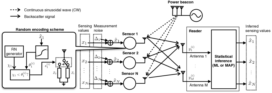
Figure 2: The design of BackSense system.

III-A random-encoding scheme

As shown in Fig. 2, the random-encoding scheme consists of the following two key steps.

Step 1) Range normalization. Distributed as a continuous variable in real domain, a measured sensing value has an infinite range. The goal of the current step is to map it to a new variable with a unit range so as to facilitate random encoding in Step 2. Consider the sensor measurement $\tilde{x}$ of a sensing value $x$. Let $\theta$ be a variable within the range $[0,1]$. Then $\tilde{x}$ can be one-to-one mapped to $\theta$ using the well-known sigmoid function (a function characterized by a S-shaped curve), denoted as $\mathcal{F}$:

$$\theta=\mathcal{F}(\tilde{x})=\frac{1}{1+\exp\left(-\frac{\tilde{x}-\mu}{\sigma}\right)},$$ (5)

where $\mu$ and $\sigma$ are mean and variance of $x$, respectively. This gives the name of $\theta$ as the mapped sensing value. It is assumed that the parameters $\mu$ and $\sigma$ are known by the sensor and reader via estimation using historical sensing data. Consider the sensing values and their measurements for all $N$ sensors, represented by the vectors $\mathbf{x}$ and $\mathbf{\tilde{x}}$, respectively, with $\mathbf{\tilde{x}}=\mathbf{x}+\boldsymbol{\Delta}$. The vector $\boldsymbol{\Delta}$ groups i.i.d. measurement-noise r.v. The element-wise mapping using (5) is represented by $\mathcal{F}(\mathbf{\tilde{x}})$, where the mapping of the $n$-th element is specified by the corresponding parameters $\mu_{n}$ and $\sigma_{n}$. The result is denoted as $\boldsymbol{\theta}$, namely $\boldsymbol{\theta}=\mathcal{F}(\mathbf{\tilde{x}})$. Since the mapping $\mathcal{F}$ is one-to-one, the mapped sensing values $\boldsymbol{\theta}$ are used in place of $\mathbf{\tilde{x}}$ in the subsequent analysis and design.

Step 2) Encoding by comparison with a uniform distributed r.v. Consider an arbitrary sensor. As shown in Fig. 2, the mapped sensing value $\theta$ is compared with a r.v., denoted as $\chi$, uniformly distributed in the same range of $[0,1]$. The r.v. is generated independently for different symbol durations. Then, the comparison yields a random sequence of binary bits for turning on/off backscattering of the sensor (see Fig. 2). The r.v. $\chi$ can be generated locally using a simple circuit (see e.g., [29, 30]). Let $S$ denote an arbitrary symbol transmitted by the sensor using on/off keying. Then $S=\bar{\rho}$ if $\chi<\theta$ or otherwise $S=0$. Thereby, the distribution of $S$ is parameterized by the mapped sensing value $\theta$ as follows:

$$S=\left\{\begin{aligned} &\bar{\rho},&&\text{w.p}\ \theta\\ &0,&&\text{w.p}\ 1-\theta.\end{aligned}\right.$$ (6)

Remark 1 (How to decode the sensing value?).

Given random encoding, the sensing value can be decoded at the reader by inferring the statistics of many observed symbols transmitted by sensors as illustrated by the following toy example case where all $N$ sensors with identical and fixed channel gains: $h_{n}^{(i)}=h$ for all $1\leq n\leq N$, $1\leq i\leq L$ and have uniform mapped sensing value $\theta$ to deliver. As a result, the reader receives a set of $L$ symbols transmitted by sensors, $\{\sum_{n=1}^{N}h_{n}^{(i)}S_{n}^{(i)}+w^{(i)}\}$, where $\{w^{(i)}\}$ represent the set of i.i.d. samples of the channel-noise process. If $L$ is sufficiently large and applying the law of large numbers, then the mapped sensing value can be recovered as

$$\theta=\lim_{L\rightarrow\infty}\frac{1}{\bar{\rho}hNL}\sum_{i=1}^{L}\sum_{n=1}^{N}h_{n}^{(i)}S_{n}^{(i)}+w^{(i)}.$$

The measured sensing value is then obtained as $\tilde{x}=\mathcal{F}^{-1}(\theta)$. The above illustration shows how the sensing value can be decoded in a simplified scenario and the performance of sensing-data uploading improves with the growth of observation duration. However, the target scenario is more complex involving practical factors including transmissions over multi-antenna channels, unknown and fluctuating channel states, spatial variation of sensing values, and finite numbers of observed symbols. This is the reason why the powerful statistical inference is needed for recovering sensing values (see Sections IV and V).

III-B Distributions of Randomized Transmissions

To facilitate statistical inference at the reader, we derive in this subsection the distributions of some r.v. arising from randomized transmissions using the proposed random-encoding scheme.

III-B1 Distribution of mapped sensing values

First, consider the case without measurement noise. For the current case, the mapping between $\boldsymbol{\theta}$ and ${\mathbf{x}}$ is one-to-one and thus $\boldsymbol{\theta}$ can be considered as an equivalence of ${\mathbf{x}}$. Using the mapping in (5), the prior distribution of $\boldsymbol{\theta}$, denoted as $p(\boldsymbol{\theta})$, can be derived based on that of ${\mathbf{x}}$, i.e., $p({\mathbf{x}})$ given in (2), as presented below.

Lemma 1.

For the case of heterogeneous sensing values without measurement noise, the distribution of $\boldsymbol{\theta}$ is specified by

$$p(\boldsymbol{\theta})=\left(\prod_{n=1}^{N}\frac{\sigma_{n}}{\theta_{n}-\theta_{n}^{2}}\right)\frac{1}{(2\pi)^{\frac{N}{2}}|\boldsymbol{\Sigma}_{\mathbf{x}}|^{\frac{1}{2}}}\exp\left(-\frac{1}{2}{\mathbf{r}}(\boldsymbol{\theta})^{T}\boldsymbol{\Sigma}_{\mathbf{x}}^{-1}{\mathbf{r}}(\boldsymbol{\theta})\right),$$ (7)

where ${\mathbf{r}}(\boldsymbol{\theta})$ is an element-wise function of $\boldsymbol{\theta}$ given by

$${\mathbf{r}}(\boldsymbol{\theta})=\left[-\sigma_{1}\log\left(\frac{1}{\theta_{1}}-1\right),\cdots,-\sigma_{N}\log\left(\frac{1}{\theta_{N}}-1\right)\right]^{T}.$$ (8)

Proof: See Appendix -A.  $\Box$

For the simplified case of uniform sensing values (all elements of ${\mathbf{x}}$ are equal), the expression given in (2) no longer holds as the covariance matrix $\boldsymbol{\Sigma}_{\mathbf{x}}$ becomes singular. Alternatively, note that ${\mathbf{x}}$ is specified by the scalar uniform value $x$ only and whose distribution can be modelled by a univariate Gaussian $x\sim{\cal N}(\mu_{0},\sigma_{0}^{2})$, where $\mu_{0}$ and $\sigma_{0}^{2}$ denote the mean and variance respectively. Thus the PDF of $x$ is then given by $p(x)=\frac{1}{\sqrt{2\pi\sigma_{0}^{2}}}\exp\left(-\frac{(x-\mu_{0})^{2}}{2\sigma_{0}^{2}}\right).$

Accordingly, following the similar procedure as for deriving Lemma 1, the distribution of $\theta={1}/\left({1+\exp\left(-\frac{x-\mu_{0}}{\sigma_{0}}\right)}\right)$ can be derived as follows:

$$p(\theta)=\frac{1}{(\theta-\theta^{2})\sqrt{2\pi}}\exp\left(-\frac{\left(\log\left(\frac{1}{\theta}-1\right)\right)^{2}}{2}\right).$$ (9)

Next, consider the case with measurement noise. For this case, the mapped sensing-value vector $\boldsymbol{\theta}$ is a function of both the sensing values ${\mathbf{x}}$ and measurement noise $\boldsymbol{\Delta}$. The randomized effect of the measurement noise on the mapping between $\boldsymbol{\theta}$ and ${\mathbf{x}}$ is captured by the conditional distribution of $\boldsymbol{\theta}$ (a latent variable) given ${\mathbf{x}}$ (a parameter) which is required in the subsequent reader inference. The result is derived using a similar method as Lemma 1 and given as follows.

Lemma 2.

For the case of heterogeneous sensing values with measurement noise, the conditional distribution function of $\boldsymbol{\theta}$ given ${\mathbf{x}}$ is given as:

$$p(\boldsymbol{\theta}|{\mathbf{x}})=\left(\prod_{n=1}^{N}\frac{\sigma_{n}}{\theta_{n}-\theta_{n}^{2}}\right)\frac{1}{(2\pi)^{\frac{N}{2}}\delta^{N}}\exp\left(-\frac{\sum_{n=1}^{N}(-\sigma_{n}\log\left(\frac{1}{\theta_{n}}-1\right)+\mu_{n}-x_{n})^{2}}{2\delta^{2}}\right).$$ (10)

III-B2 Distribution of the number of active sensors

A latent variable that affects the distribution of received signal at the reader is the number of active (on) sensors, denoted as $T^{(i)}$ for the $i$-th slot (see Fig. 3 and 4). Given on/off keying, $T^{(i)}$ is the sum over a sequence of Bernoulli r.v. that represent the $i$-th symbols transmitted by all sensors: $T^{(i)}=\sum_{n=1}^{N}S^{(i)}_{n}$ where $\{S^{(i)}_{n}\}$ follow the distribution in (6). Consider the case where the mapped sensing values differ over sensors, denoted as $\theta_{1},\theta_{2},\cdots,\theta_{N}$. The r.v. is a Poisson-Binomial r.v. that describes the numbers of successes in $N$ independent Bernoulli trails with different individual success probabilities, denoted by ${\cal PB}(N,\theta_{1},\theta_{2},\cdots,\theta_{N})$. The corresponding probability mass function (PMF) is given as [31]:

$$p(T^{(i)}=m|\boldsymbol{\theta})=\frac{1}{N+1}\sum_{\ell=0}^{N}c^{-\ell m}\prod_{n=1}^{N}[1+(c^{\ell}-1)\theta_{n}],\qquad m=0,1,\cdots,N,$$ (11)

where $c=\exp\left(\frac{2\pi j}{N+1}\right)$ with $j=\sqrt{-1}$. For the special case of uniform mapped sensing values denoted as $\theta$, the distribution of $T^{(i)}$ reduces to the Binomial distribution:

$$p(T^{(i)}=m|\theta)={N\choose m}\theta^{m}(1-\theta)^{N-m},\qquad m=0,1,\cdots,N.$$ (12)

IV BackSense Design: Reader Inference with Ideal Measurements

This section addresses the design problem of reader inference formulated in Section II-B2. To this end, statistical inference algorithms are designed based on the EM framework, which enable the reader to recover the sensing values form the received signals. Ideal measurements are assumed and the effect of measurement noise on the design is addressed in the next section. We start with a brief introduction to the basic principle of the EM framework. Then a Bayesian network is constructed for specifying the statistical dependencies between the observations and unknowns (including the latent variables and model parameters). Based on the Bayesian network, EM algorithms targeting BackSense are designed for both the criteria of ML and MAP.

IV-A Principle of the EM Framework

Due to the existence of latent variables, directly solving the potentially non-convex ML and MAP problems formulated in Section II-B2 is intractable. Alternatively, the EM framework tempts to find local-optimal solutions by an iterative procedure, involving iterations between two main steps, i.e., the Expectation step (E-step) and the Maximization step (M-step) (see e.g., [32]). In the E-step, the expectation of the complete-data log likelihood is used as a surrogate of the required incomplete-data log likelihood as defined later. Then in the M-step, the surrogate is maximized instead of the actual incomplete-data log likelihood. The use of the surrogate makes finding the solution more tractable without compromizing its local-optimality. For exposition, the details are discussed in the sequel based on the ML criterion while the same principle also applies to the MAP criterion.

Assume that we have $L$ i.i.d. observations. We denote all of the observed variables as ${\mathbf{Y}}=[{\mathbf{y}}^{(1)},{\mathbf{y}}^{(2)},\cdots,{\mathbf{y}}^{(L)}]$, all of the latent variables as ${\mathbf{Z}}=[{\mathbf{z}}^{(1)},{\mathbf{z}}^{(2)},\cdots,{\mathbf{z}}^{(L)}]$, and all of the parameters as $\bf\Phi$. By introducing an auxiliary distribution $q({\mathbf{Z}})$ defined over the latent variables ${\mathbf{Z}}$, the incomplete-data log likelihood can be decomposed by

$$\log p({\mathbf{Y}}|{\bf\Phi})={\cal L}(q,{\bf\Phi})+\text{KL}(q||p),$$ (13)

where ${\cal L}(q,{\bf\Phi})={\int}q({\mathbf{Z}})\log\left\{\frac{p({\mathbf{Y}},{\mathbf{Z}}|{\bf\Phi})}{q({\mathbf{Z}})}\right\}{\text{d}}{{\mathbf{Z}}}$ is the expectation of the complete-data log likelihood and the $\text{KL}(q||p)=-\int q({\mathbf{Z}})\log\left\{\frac{p({\mathbf{Z}}|{\mathbf{Y}},{\bf\Phi})}{q({\mathbf{Z}})}\right\}{\text{d}}{{\mathbf{Z}}}$ is known as Kullback-Leibler (KL) divergence. Note that the KL divergence measures the “similarity” between the two distributions of $q$ and $p$. Hence the measure is a non-negative function attaining the minimum when $q$ and $p$ are identically distributed. Therefore, it follows from (13) that ${\cal L}(q,{\bf\Phi})$ lower bounds $\log p({\mathbf{Y}}|{\bf\Phi})$. One can see that the bound reaches equality, namely $\text{KL}(q||p)=0$, by letting $q({\mathbf{Z}})=p({\mathbf{Z}}|{\mathbf{Y}},{\bf\Phi})$. This essentially gives the E-step. The resultant tight lower bound can then serve as a surrogate of $\log p({\mathbf{Y}}|{\bf\Phi})$ that is optimized to provide updated parameters $\bf\Phi$, constituting the M-step. As a result, the maximization of (13) can be solved by repeating the following EM cycle, where the subscript $(t)$ is used to denote the iteration index:

$${\bf E\!-\!step}:\qquad q^{(t+1)}({\mathbf{Z}})\leftarrow\arg\max_{q}{\cal L}(q,{\bf\Phi}^{(t)})$$ (14)

$$\implies q^{(t+1)}({\mathbf{Z}})=p({\mathbf{Z}}|{\mathbf{Y}},{\bf\Phi}^{(t)}).$$ (15)

$${\bf M\!-\!step}:\qquad {\bf\Phi}^{(t+1)}\leftarrow\arg\max_{\bf\Phi}{\cal L}(q^{(t+1)},{\bf\Phi})$$ (16)

$$\implies {\bf\Phi}^{(t+1)}\leftarrow\arg\max_{\bf\Phi}\int p({\mathbf{Z}}|{\mathbf{Y}},{\bf\Phi}^{(t)})\log p({\mathbf{Y}},{\mathbf{Z}}|{\bf\Phi}^{(t)}){\text{d}}{\mathbf{Z}}.$$ (17)

The above EM cycle starts from some initial values for the parameters ${\bf\Phi}$ and keep repeating until convergence. The convergence of the EM framework to at least a local optimum is guaranteed since both the E-step (14) and M-step (16) lead to a non-decreasing objective ${\cal L}(q,{\bf\Phi})$ at each EM cycle [32].

IV-B Construction of Bayesian Network

Designing the BackSense inference algorithms begins with constructing a Bayesian network that specifies the set of parameters and latent variables affecting the received signal as well as their interdependence characterized by their conditional distributions. The set of parameters are unknown to the readers and thus the target of inference. The parameter set $\bf\Phi$ comprises the mapped sensing values $\boldsymbol{\theta}$, channel variance $\sigma_{h}^{2}$ and channel-noise variance $\sigma_{w}^{2}$: ${\bf\Phi}=\{{\boldsymbol{\theta}},\sigma_{h}^{2},\sigma_{w}^{2}\}$. For the current case without measurement noise, there exists only one type of latent variables, namely the set of randomized symbols transmitted by sensors, that affect the observed variable, namely the received symbols over multiple antennas.

Consider the $i$-th slot. To complete the construction of the Bayesian network, the conditional distribution of the received symbol vector ${\mathbf{y}}^{(i)}$ given the transmitted symbol vector ${\mathbf{s}}^{(i)}$ is derived as follows. Note that the elements of the additive noise and the channel matrix in (1) are complex Gaussians. It follows from (1) that given ${\mathbf{s}}^{(i)}$, ${\mathbf{y}}^{(i)}$ is a sum of complex Gaussian vectors that also follows the complex Gaussian distribution. Specifically, conditioned on ${\mathbf{s}}^{(i)}$, ${\mathbf{y}}^{(i)}\sim{\cal CN}(0,\sigma_{h}^{2}\sum_{n=1}^{N}S^{(i)}_{n}+\sigma_{w}^{2})$. One can see that given on/off keying for sensor transmissions, the sum $\sigma_{h}^{2}\sum_{n=1}^{N}S^{(i)}_{n}$ is equal to $\bar{\rho}T^{(i)}$ where $T^{(i)}$ is the number of active tags and $\bar{\rho}$ is the reflection coefficient for an active sensor. Without loss of generality, we set $\bar{\rho}=1$ in the subsequent analysis for ease of notation. Mathematically,

$$p(\mathbf{y}^{(i)}\mid{\mathbf{s}}^{(i)})=p(\mathbf{y}^{(i)}\mid T^{(i)})=\frac{1}{\left[2\pi(\sigma_{h}^{2}T^{(i)}+\sigma_{w}^{2})\right]^{M}}\exp\left(-\frac{{\|\mathbf{y}^{(i)}\|_{2}^{2}}}{2(\sigma_{h}^{2}T^{(i)}+\sigma_{w}^{2})}\right).$$ (18)

This suggests that the latent variable ${\mathbf{s}}^{(i)}$ can be replaced with $T^{(i)}$ without changing the distribution of ${\mathbf{y}}^{(i)}$. The distribution of $T^{(i)}$ is derived earlier as given in (11) and (12). Note that the variable replacement reduces the dimensions of latent space from $N$ to just $1$, reducing the complexity of inference. Based on the above discussion, the Bayesian network corresponding to the $i$-th received symbol is illustrated in Fig. 3.

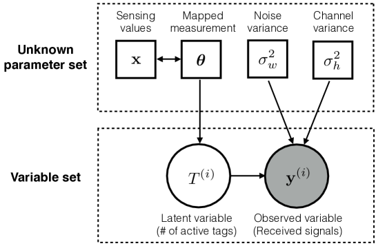
Figure 3: Bayesian network for BackSense inference without measurement noise.

IV-C Reader ML Inference with Uniform Sensing Values

In this subsection, we consider the simple case of uniform sensing values $\theta$ and the ML criterion for designing the reader-inference algorithm. The design is subsequently extended to the case of heterogeneous sensing values as well as the MAP criterion. Based on the EM framework introduced in Section IV-A, the algorithm for inferring $\theta$ is designed for BackSense by driving the corresponding E-step and M-step shortly. The resultant procedure is summarized in Algorithm 1. Given the inferred sensing value $\hat{\theta}$ and the mapping in (5), the inferred sensing value is then obtained as

$$\hat{x}=\sigma_{0}\log\left(\frac{1}{\hat{\theta}}-1\right)+\mu_{0}.$$ (19)

a) Derivation of E-step
Consider the Bayesian network in Fig. 3. Given the parameter set ${\bf\Phi}_{\sf uni}=\{\theta,\sigma_{h}^{2},\sigma_{w}^{2}\}$, the required posterior distribution of the latent variable $T^{(i)}$ can be computed via Bayes’ Law as

$$q(T^{(i)}=m)=p(T^{(i)}=m\mid{\mathbf{y}}^{(i)},{\bf\Phi}_{\sf uni})=\frac{f_{m}}{\sum_{n}f_{n}},$$ (20)

where $f_{m}$ is defined as

$$f_{m}=\frac{1}{\left[2\pi(\sigma_{h}^{2}m+\sigma_{w}^{2})\right]^{M}}\exp\left(-\frac{{\|{{\mathbf{y}}^{(i)}}\|_{2}^{2}}}{2(\sigma_{h}^{2}m+\sigma_{w}^{2})}\right){N\choose m}\theta^{m}(1-\theta)^{N-m},\;\;m=0,1,\cdots,N.$$ (21)

This completes the derivation of the E-step as indicated in (15). For ease of notation, let $q^{(i)}_{T}(m)$ denote $q(T^{(i)}=m)$ in the rest of the paper.

Initialization:

Initialize the model parameters $\theta$, $\sigma_{h}^{2}$, $\sigma_{w}^{2}$ properly.

Iteration:

1) E-step: Update the posterior distribution of the latent variable, $\{q^{(i)}_{T}(m)\}$, according to (20).

2) M-step: Update the parameter $\theta$ and $\sigma_{h}^{2}$, $\sigma_{w}^{2}$ by substituting the latest values of $\{q^{(i)}_{T}(m)\}$ into (25) and (29), respectively.

Until Convergence.

Algorithm 1 EM algorithm for ML reader inference

b) Derivation of M-step
According to the M-step in (17), the parameter set ${\bf\Phi}_{\sf uni}$ should be optimized by solving

$${\bf\Phi}_{\sf uni}^{*}=\arg\max_{{\bf\Phi}_{\sf uni}}\sum_{i=1}^{L}\sum_{m=0}^{N}q^{(i)}_{T}(m)\log p({\mathbf{y}}^{(i)},T^{(i)}=m\mid{{\bf\Phi}_{\sf uni}}),$$ (22)

where the joint distribution over the observed and latent variables is given by

$$p({\mathbf{y}}^{(i)},T^{(i)}=m\mid{{\bf\Phi}_{\sf uni}})=f_{m},\qquad m=0,1,\cdots,N,$$ (23)

where $f_{m}$ is defined in (21). Recall that the parameter set ${\bf\Phi}_{\sf uni}=\{\theta,\sigma_{h}^{2},\sigma_{w}^{2}\}$. A close observation of (22) and (23) reveals that $\theta$ and $\{\sigma_{w}^{2},\sigma_{h}^{2}\}$ are decoupled in the objective function in (22) and thereby they can be optimized separately.

Firstly, we derive the updating formula for the parameter $\theta$ by considering those terms in (22) that are related to $\theta$ only, the corresponding optimization problem is given as

$$\theta^{*}=\arg\max_{\theta\in(0,1)}\sum_{i=1}^{L}\sum_{m=0}^{N}q^{(i)}_{T}(m)[m\log\theta+(N-m)\log(1-\theta)],$$ (24)

Proposition 1.A.

The value of $\theta$ that solves the optimization problem in (24) is given by

$$\theta^{*}=\frac{1}{LN}{\sum_{i=1}^{L}\sum_{m=1}^{N}q^{(i)}_{T}(m)m}.$$ (25)

Proof: See Appendix -B.  $\Box$

The above result yields the formula for updating the parameter $\theta$ in the M-step.

Next, to derive the updating formula for the parameters $\sigma_{w}^{2}$ and $\sigma_{h}^{2}$ , group the relevant terms in the objective function in (22). The corresponding optimization problem is

$$\max_{\sigma_{h}^{2},\sigma_{w}^{2}}\sum_{i=1}^{L}\sum_{m=0}^{N}q^{(i)}_{T}(m)\left[-M\log(\sigma_{h}^{2}m+\sigma_{w}^{2})-\frac{\|{{\mathbf{y}}^{(i)}}\|_{2}^{2}}{2(\sigma_{h}^{2}m+\sigma_{w}^{2})}\right].$$ (26)

The problem is non-convex and thus it is difficult to find its solution in closed form. To overcome the difficulty, we develop a sub-optimal approach that relaxes the problem to a quasiconvex one and solving it provides closed-form updates for the target parameters $\sigma_{h}^{2}$ and $\sigma_{w}^{2}$. For this purpose, one can observe that the objective function depends on $\sigma_{h}^{2}$ and $\sigma_{w}^{2}$ via a weighted sum, defined as $\Sigma_{m}=\sigma_{h}^{2}m+\sigma_{w}^{2}$. By substituting $\Sigma_{m}$, the optimization problem in (26) is converted to the following quasiconvex problem:

$$\max_{\{\Sigma_{m}\}}\sum_{i=1}^{L}\sum_{m=0}^{N}q^{(i)}_{T}(m)\left(-M\log(\Sigma_{m})-\frac{\|{{\mathbf{y}}^{(i)}}\|_{2}^{2}}{2\Sigma_{m}}\right).$$ (27)

Proposition 1.B.

The optimal values of $\{\Sigma_{m}\}$ that solve the problem in (27) are given by

$$\Sigma_{m}^{*}=\frac{\sum_{i=1}^{L}q^{(i)}_{T}(m)\|{{\mathbf{y}}^{(i)}}\|_{2}^{2}}{2M\sum_{i=1}^{L}q^{(i)}_{T}(m)},\qquad m=0,1,\cdots,N.$$ (28)

Proof: See Appendix -C.  $\Box$

Note that in general, it is infeasible to find the values of $\sigma_{h}^{2}$ and $\sigma_{w}^{2}$ that satisfy $(N+1)$ equations: $\Sigma_{m}=\sigma_{h}^{2}m+\sigma_{w}^{2}$ with $m=0,1,\cdots,N$. Thus, we resort to finding approximate values, denoted as $(\sigma_{w}^{2*},\sigma_{h}^{2*})$, by linear regression:

$$(\sigma_{h}^{2*},\sigma_{w}^{2*}) =\arg\min_{(\sigma_{w}^{2},\sigma_{h}^{2})}\sum_{m=0}^{N}\left(\sigma_{w}^{2}+m\sigma_{h}^{2}-\Sigma_{m}^{*}\right)^{2}$$

$$=\left(\frac{\sum_{m=0}^{N}(m-\frac{N}{2})(\Sigma_{m}^{*}-\bar{\Sigma})}{\sum_{m=0}^{N}(m-\frac{N}{2})^{2}},\bar{\Sigma}-\frac{N}{2}\sigma_{h}^{2*}\right)$$ (29)

where $\bar{\Sigma}$ denotes the mean of the optimal values of $\{\Sigma_{m}^{*}\}$ derived in (28). The above result gives the formula for updating the parameters $\sigma_{h}^{2}$ and $\sigma_{w}^{2}$ for the M-step. Combining this result and that in Proposition 1.A completes the derivation of the M-step.

IV-D Extension: Reader MAP Inference

The EM algorithm based on the ML criterion as shown in Algorithm 1 is extended to the MAP criterion as follows. Comparing (3) and (4), one can see that the objective function for the MAP problem differs from the ML counterpart only by the extra term $\log p(\boldsymbol{\Phi})$, corresponding to the “log-prior” of the unknown parameters. Thus, deriving the MAP algorithm requires only modifying the M-step of the ML counterpart that updates the estimation of the parameters. Specifically, the M-step for the MAP algorithm can be written as

$$\boldsymbol{\Phi}_{\sf uni}^{*}=\arg\max_{{\bf\Phi}_{\sf uni}}\sum_{i=1}^{L}\sum_{m=0}^{N}q^{(i)}_{T}(m)\log p({\mathbf{y}}^{(i)},T^{(i)}=m\mid{{\bf\Phi}_{\sf uni}})+\log p({\bf\Phi}_{\sf uni}).$$ (30)

Recall that $\boldsymbol{\Phi}_{\sf uni}=\{\theta,\sigma_{h}^{2},\sigma_{w}^{2}\}$. The prior distribution of $\theta$ is derived as shown in (9). However, for those of $\sigma_{h}^{2}$ and $\sigma_{w}^{2}$, in practice, such information is difficult to obtain from historical inference results or estimate due to lack of training signals. A common technique to tackle the difficulty is to replace the required prior distributions with some constants, known as non-informative priors (see e.g., [33]). To some extent, the technique reduces the performance gain of MAP interference over ML inference. Using the technique and prior distribution of $\theta$ in (9), the optimization problem for updating $\theta$ in the M-step for the MAP inference is modified from the ML counterpart in (24) as

$$\max_{\theta\in(0,1)}\sum_{i=1}^{L}\sum_{m=0}^{N}q^{(i)}_{T}(m)[m\log\theta+(N-m)\log(1-\theta)]-\log\theta(1-\theta)-\frac{\left[\log\left(\frac{1}{\theta}-1\right)\right]^{2}}{2}.$$ (31)

Proposition 2.

The optimal value of $\theta$ that solves the optimization problem in (31) satisfies

$$e^{(LN-2)\theta^{*}}=a\left(\frac{1}{\theta^{*}}-1\right),$$ (32)

where $a$ is a constant and given by $a=\exp\left(\sum_{i=1}^{L}\sum_{m=0}^{N}q^{(i)}_{T}(m)m-1\right)$.

The proof is straightforward and omitted here for brevity. Though $\theta^{*}$ has no closed form, it can be computed by a simple numerical search. On the other hand, due to the use of non-informative priors, the procedure for updating the other parameters, i.e., $\sigma_{h}^{2}$ and $\sigma_{w}^{2}$, remains the same as the ML counterpart.

In summary, the iterative algorithm for MAP inference for the current case can be modified from Algorithm 1 by replacing (25) in Step 2) with solving the equation in (32).

Remark 2.

(ML versus MAP) A comparison between (22) and (30) reveals that, for MAP inference, the reader’s knowledge of parameters’ prior distributions servers as an additional regularization term in the objective function to avoid overfitting to the potential outliers in the data set. This makes the performance more robust even when there are errorneous data points in the data set or its size is not large enough.

IV-E Extension: Heterogeneous Sensing Values

In the preceding sub-sections, we designed inference algorithms for the simple case of uniform sensing values. They are extended in this sub-section to the general case of heterogeneous sensing values. The corresponding parameter $\boldsymbol{\theta}$ is a vector comprising $N$ elements instead of being a scalar in the preceding case. Their joint distribution is derived earlier as shown in (7). Given their relation shown in Fig. 3, the change in $\boldsymbol{\theta}$ causes the number of active tags, $T^{(i)}$, to follow the Poisson-Binomial distribution in (11) instead of the Binomial distribution in the case of uniform sensing values. The above changes in parametric distributions require the EM algorithms for reader inference to be modified as follows.

a) Derivation of E-step
According to (15), given initial values of the unknown parameters ${\bf\Phi}_{\sf cor}=\{\boldsymbol{\theta},\sigma_{h}^{2},\sigma_{w}^{2}\}$, the E-step calculates the posterior distribution of the latent variable by Bayes’ law as follows.

$$q(T^{(i)}=m) =p(T^{(i)}=m\mid{\mathbf{y}}^{(i)},{\bf\Phi}_{\sf cor})=\frac{g_{m}}{\sum_{n}g_{n}},$$ (33)

where $g_{m}$ with $m=0,1,\cdots,N$ is defined as

$$g_{m} =\frac{1}{\left[2\pi(\sigma_{h}^{2}m+\sigma_{w}^{2})\right]^{M}}\exp\left(-\frac{{\|{{\mathbf{y}}^{(i)}}\|_{2}^{2}}}{2(\sigma_{h}^{2}m+\sigma_{w}^{2})}\right)\frac{1}{N+1}\sum\limits_{\ell=0}^{N}c^{-\ell m}\prod_{n=1}^{N}[1+(c^{\ell}-1)\theta_{n}].$$ (34)

b) Derivation of M-step
The formulas for updating the parameters $\sigma_{w}^{2}$ and $\sigma_{h}^{2}$ remain the same as in (29). Only that for updating $\boldsymbol{\theta}$ needs to be modified as follows. Similar to (24), by considering only those terms related to $\boldsymbol{\theta}$ in the M-step optimization, the update of $\boldsymbol{\theta}$ requires to solve the following two optimization problems based on the ML and MAP criteria, respectively:

(ML) $$\max_{\boldsymbol{\theta}}\tilde{g}(\boldsymbol{\theta}),$$ (35)

(MAP) $$\max_{\boldsymbol{\theta}}\left[\tilde{g}(\boldsymbol{\theta})-\sum_{n=1}^{N}\log(\theta_{n}-\theta_{n}^{2})-\frac{1}{2}{\mathbf{r}}(\boldsymbol{\theta})^{T}\boldsymbol{\Sigma}_{\mathbf{x}}^{-1}{\mathbf{r}}(\boldsymbol{\theta})\right],$$ (36)

where $\tilde{g}(\boldsymbol{\theta})$ is defined as

$$\tilde{g}(\boldsymbol{\theta})=\sum_{i=1}^{L}\sum_{m=0}^{N}q^{(i)}_{T}(m)\log\left\{\sum_{\ell=0}^{N}c^{-\ell m}\prod_{n=1}^{N}[1+(c^{\ell}-1)\theta_{n}]\right\}.$$ (37)

It can be observed from the above two optimization problems that the mapped sensing values $\{\theta_{n}\}$ are coupled with each other, making the problem non-convex and the direct solutions intractable. In the area of statistical inference, a common approach for tackling this challenge, known as the generalized EM (GEM) framework (see e.g., [34]), is to update the parameters in a tractable way to increase the M-step objective in (35) or (36) (e.g., using gradient ascent) instead of exactly maximizing it. Using this technique, each complete EM cycle of the GEM algorithm is guaranteed to increase the value of the log likelihood objective until converging to a local optimum [34]. Specifically, the iterative equation for updating ${\boldsymbol{\theta}}$ can be derived as shown below:

$$\boldsymbol{\theta}^{(t+1)}=\boldsymbol{\theta}^{(t)}+\alpha\nabla\mathcal{L}(\boldsymbol{\theta}^{(t)}),$$ (38)

where $\alpha$ is the step size and $\nabla\mathcal{L}(\boldsymbol{\theta})$ denotes the derivative of the objective function in either (35) or (36), representing the gradient direction, and whose the $n$-th element is given by:

$$\left[\nabla\mathcal{L}(\boldsymbol{\theta})\right]_{n}(\text{ML}) =\sum_{i=1}^{L}\sum_{m=0}^{N}q^{(i)}_{T}(m)\frac{\sum_{\ell=0}^{N}c^{-\ell m}(c^{\ell}-1)\prod_{n^{\prime}\neq n}^{N}[1+(c^{\ell}-1)\theta_{n^{\prime}}]}{\sum_{\ell=0}^{N}c^{-\ell m}\prod_{n=1}^{N}[1+(c^{\ell}-1)\theta_{n}]}.$$ (39)

$$\left[\nabla\mathcal{L}(\boldsymbol{\theta})\right]_{n}(\text{MAP}) =\left[\nabla_{\boldsymbol{\theta}}\tilde{\cal L}(\boldsymbol{\theta})\right]_{n}(\text{ML})-\frac{1-2\theta_{n}}{\theta_{n}(1-\theta_{n})}-\frac{\sigma_{n}}{(\theta_{n}-\theta_{n}^{2})}\left[\boldsymbol{\Sigma}_{\mathbf{x}}^{-1}{\mathbf{r}}(\boldsymbol{\theta})\right]_{n}.$$ (40)

In summary, the iterative algorithm for reader inference in the current case can be modified from Algorithm 1 by simply replacing (20) in the E-step with (33) and (25) in M-step with (38).

V BackSense Design: Reader Inference with Noisy Measurements

In the preceding section, the mapped sensing value vector $\boldsymbol{\theta}$ is a parameter in the Bayesian network (see Fig. 3) since it is one-to-one mapped from the sensing-value vector ${\mathbf{x}}$ and remains fixed throughout the observation duration. In this section, in the presence of measurement noise, $\boldsymbol{\theta}$ is a random vector conditioned on ${\mathbf{x}}$ and varies from symbol-to-symbol, making it a latent variable in the Bayesian network. This causes the dimensionality of the latent space increasing linearly with the number of sensors. To overcome the resultant prohibitive complexity of statistical inference for a large number of sensors, we design practical approximate EM algorithms using the method of variational inference. The details are presented targeting ML inference. The extension to the MAP inference is straightforward and omitted for brevity.

V-A Construction of Bayesian Network

With the addition of measurement noise, the corresponding Bayesian network is modified from the noise-free counterpart (see Fig. 3) as shown in Fig. 4 and described as follows. First of all, the mapped sensing vector $\boldsymbol{\theta}^{(i)}$ is changed from a parameter to a latent variable. Moreover, an extra parameter $\delta^{2}$, namely the measurement-noise variance, is included that affects the latent variable $\boldsymbol{\theta}^{(i)}$ together with the sensing-value vector ${\mathbf{x}}$. The corresponding conditional distribution of $\boldsymbol{\theta}^{(i)}$ for given $\delta^{2}$ and ${\mathbf{x}}$ is derived earlier as shown in (10). On the other hand, the conditional distributions of the other latent variable $T^{(i)}$ and the observed variable ${\mathbf{y}}^{(i)}$ are identical as their measurement-noise-free counterparts given in (11) and (18), respectively.

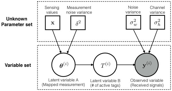
Figure 4: Bayesian network for BacksSense with the measurement noise.

V-B Reader Inference Based on Approximate EM Implementation

V-B1 Principle of the Variational Inference

The method of variation inference is one low-complexity approximation of the EM framework. The key idea is to apply the mean field theory [35] that constrains the variational distribution $q({\mathbf{Z}})$ in the EM framework [see (14): E-step and (16): M-step] to belong to a family of distribution functions charaterized by the factorized form $q({\mathbf{Z}})=\prod_{k}q_{k}({\mathbf{z}}_{k})$, where ${\mathbf{z}}_{k}^{T}$ is the $k$-th row of ${\mathbf{Z}}$ and $q_{k}$ is the corresponding factor function [28]. When a Bayesian network can be decoupled into sub-networks or the complete data likelihood can be factorized into product form, the approximation can reduce integrals over a high-dimensional latent space to multiple parallel integrals with low dimensionality and hence low complexity. By substituting the approximate form of $q({\mathbf{Z}})=\prod_{k}q_{k}({\mathbf{z}}_{k})$, the two steps of EM framework in (15) and (17) can be modified and written as follows [28]:

$${\bf Variational\;\;E\!-\!step}:\quad q^{(t+1)}({\mathbf{Z}})=b\prod_{\ell}\exp\left(\int\log p\left({\mathbf{Y}},{\mathbf{Z}}|{\bf\Phi}^{(t)}\right)\prod_{k\neq\ell}q_{k}({\mathbf{z}}_{k})d{\mathbf{z}}_{k}\right),$$ (41)

$${\bf Variational\;\;M\!-\!step}:\quad {\bf\Phi}^{(t+1)}\leftarrow\arg\max_{\bf\Phi}\int q^{(t+1)}({\mathbf{Z}})\log p({\mathbf{Y}},{\mathbf{Z}}|{\bf\Phi}^{(t)}){\text{d}}{\mathbf{Z}},$$ (42)

where $b$ is a normalization constant whose value can be computed by inspection. One can observe from (41) and (42) that the high-dimensional integrals therein can be reduced into low-dimensional ones if the term $p\left({\mathbf{Y}},{\mathbf{Z}}|{\bf\Phi}^{(t)}\right)$ can be decomposed as the product of factors that are functions of non-overlapping subsets of the rows of ${\mathbf{Z}}$.

V-B2 Inference Algorithm Derivation

Based on the Bayesian network in Fig. 4 and applying the mean field approximation, the variational distribution in the EM framework is constrained to take the fully factorized form $q({\mathbf{z}}^{(i)})=q(T^{(i)})\prod_{n}q(\theta_{n}^{(i)})$. Then according to (41) we have

$$q^{*}(T^{(i)}) =b_{0}\exp\left\{\mathbb{E}_{\boldsymbol{\theta}}\left[\log p({\mathbf{y}}^{(i)},T^{(i)},\boldsymbol{\theta}^{(i)}\mid{\bf\Phi}_{\sf noi})\right]\right\},$$ (43)

$$q^{*}(\theta_{n}^{(i)}) =b_{n}\exp\left\{\mathbb{E}_{T,\boldsymbol{\theta}\backslash\theta_{n}}\left[\log p({\mathbf{y}}^{(i)},T^{(i)},\boldsymbol{\theta}^{(i)}\mid{\bf\Phi}_{\sf noi})\right]\right\},\qquad\forall n,$$ (44)

where $\{b_{n}\}$ are normalization constants. The explicit expressions of the approximate marginal distributions of individual latent variables shown in (43) and (44) can be derived based on the following procedure. Considering (43), apply the conditional distributions derived earlier as shown in (10), (11), (18) and together with the chain rule, followed by separating the terms depending on $T$ in (43) from those on $\theta_{n}$. Similar procedure can be applied to (44). As the result, we can obtain the said marginal distributions as shown below, giving the variational E-step.

Proposition 3.A.

The variational E-step involves calculation of the approximate marginal distributions of latent variables given as:

$$q^{*}(T^{(i)}=m)=\frac{g_{a}(m)}{\sum_{k}g_{a}(k)},\qquad q^{*}(\theta_{n}^{(i)}=z_{n})=\frac{g_{b}(z_{n})}{\int_{0}^{1}g_{b}(z_{n})dz_{n}},\;\;\forall n,$$ (45)

where $g_{a}(m)$ and $g_{b}(z_{n})$ are given as

$$g_{a}(m) =\frac{\mathcal{F}_{1}(m)}{\sigma^{2}_{w}+m\sigma_{h}^{2}}\exp\left\{-\frac{\|{\mathbf{y}}^{(i)}\|_{2}^{2}}{2(\sigma^{2}_{w}+m\sigma_{h}^{2})}\right\},$$

$$g_{b}(z_{n}) =\frac{\mathcal{F}_{2}(z_{n})}{z_{n}(1-z_{n})}\exp\left\{-\frac{1}{2\delta^{2}}\left(-\sigma_{n}\log\left(\frac{1}{z_{n}}-1\right)+\mu_{n}-x_{n}\right)^{2}\right\},$$

wherein we define two functions for ease of notation:

$$\mathcal{F}_{1}(m) =\exp\left\{\mathbb{E}_{\boldsymbol{\theta}}\left(\log\left(\sum\nolimits_{\ell=0}^{N}c^{-\ell m}\prod\nolimits_{k=1}^{N}[1+(c^{\ell}-1)\theta_{k}]\right)\right)\right\}.$$ (46)

$$\mathcal{F}_{2}(z_{n}) =\left.\exp\left\{\mathbb{E}_{T,\boldsymbol{\theta}\backslash\theta_{n}}\left(\log\left(\sum\nolimits_{\ell=0}^{N}c^{-\ell T}\prod\nolimits_{k=1}^{N}[1+(c^{\ell}-1)\theta_{k}]\right)\right)\right\}\right|_{\theta_{n}=z_{n}}.$$ (47)

Next, we derive the variational M-step. To this end, substitute the marginal distributions of latent variables in (45) into (42), and solve the resultant optimization problems. Thereby, we have the following set of equations for parametric updating, constituting the variational M-step.

Proposition 3.B.

For the variational M-step, the parameters $\{{\mathbf{x}},\delta^{2},\sigma^{2}_{h},\sigma_{w}^{2}\}$ are updated as:

$$x_{n}^{*} =\mu_{n}-\frac{1}{L}\sum_{i=1}^{L}\int q(\theta_{n}^{(i)})\sigma_{n}\log\left({1}/{\theta_{n}^{(i)}}-1\right)\text{d}\theta_{n}^{(i)}\qquad n=1,2,\cdots,N.$$

$${\delta^{2}}^{*} =\frac{1}{LN}\sum_{i=1}^{L}\sum_{n=1}^{N}\int q(\theta_{n}^{(i)})(-\sigma_{n}\log(1/\theta_{n}^{(i)}-1)+\mu_{n}-x_{n})^{2}\text{d}\theta_{n}^{(i)}.$$

$$\Sigma_{m}^{*} =\frac{\sum_{i=1}^{L}q(T^{(i)}=m)\|{{\mathbf{y}}^{(i)}}\|_{2}^{2}}{2M\sum_{i=1}^{L}q(T^{(i)}=m)},\qquad m=0,1,\cdots,N$$

$$(\sigma^{2*}_{h},\sigma_{w}^{2*}) =\left(\frac{\sum_{m=0}^{N}(m-\frac{N}{2})(\Sigma_{m}^{*}-\bar{\Sigma})}{\sum_{m=0}^{N}(m-\frac{N}{2})^{2}},\bar{\Sigma}-\frac{N}{2}\sigma_{h}^{2*}\right)$$

Finally, the main steps of the approximate EM algorithm is summarized in Algorithm 2.

Remark 3.

(Complexity Reduction by Variational Inference) It can be observed from Proposition 3.B that only one-dimension integrals are required in the variational M-step. However, high dimension integrals are still needed in the variational E-step (see Proposition 3.A) for the reason that given the parameters, the joint distribution function of observation and latent variables cannot be decomposed into the fully factorized form. Despite this, the method of variation inference still leads to substantial complexity reduction with respect to the exact EM inference where both the E-step and M-step involve $N$-dimension integrals over the full latent space.

Initialization:

Initialize the model parameters ${\mathbf{x}}$, $\delta^{2}$, $\sigma_{h}^{2}$, $\sigma_{w}^{2}$, and the marginal posteriors $q(T^{(i)})$ and $\{q(\theta_{n}^{(i)})\}$; Iteration:

1) E-step: Compute the approximate marginal posteriors of latent variables iteratively by cycling the variational distributions presented in (45) in Proposition 3.A for rounds until convergence;

2) M-step: Update the parameters according to the formulas in Proposition 3.B;

Until Convergence.

Algorithm 2 Summary of the approximate EM algorithm using variational inference

VI Simulation Results

For simulation, the performance metric is the inference error, defined by $\frac{\|\hat{\mathbf{x}}-{\mathbf{x}}\|}{\|{\mathbf{x}}\|}$. The simulation parameters are set as follows unless specified otherwise. The average transmit signal-and-noise ratio (SNR), defined as ${P_{t}}/{\sigma_{w}^{2}}$, is set to be $10$ dB. The variances of the wireless channel and the additive Gaussian noise are $\sigma_{h}^{2}=\sigma_{w}^{2}=1$. For the prior distribution of ${\mathbf{x}}$, the mean is $\mu_{n}=25,\forall n$, and the covariance matrix $\boldsymbol{\Sigma}_{\mathbf{x}}$ can be decomposed as $\boldsymbol{\Sigma}_{\mathbf{x}}$ = ${\mathbf{D}}^{1/2}{\mathbf{C}}_{\mathbf{x}}{\mathbf{D}}^{1/2}$, where ${\mathbf{D}}$ is a diagonal matrix with the diagonal elements collecting the variances of the elements of ${\mathbf{x}}$, namely $[{\mathbf{D}}]_{n,n}=\sigma_{n}^{2}$, and we set $\sigma_{n}^{2}=1,\forall n$. Moreover, the correlation matrix ${\mathbf{C}}_{\mathbf{x}}$ is assumed to have the linear exponent autoregressive structure [36]:

$${\mathbf{C}}_{\mathbf{x}}=\left[{\begin{array}[]{*{20}{c}}1&\rho&{{\rho^{2}}}&\cdots&{{\rho^{N-1}}}\\ \rho&1&\rho&\cdots&{\rho^{N-2}}\\ \vdots&\vdots&\vdots&{}\hfil&\vdots\\ \rho^{N-1}&\rho^{N-2}&\rho^{N-3}&\cdots&1\end{array}}\right],$$ (52)

in which the parameter $\rho\in[0,1)$ controls the level of correlation between the adjacent sensor tags, the correlation between tags further away is assumed to decrease with the growth of their spatial separation following a geometric sequence $1,\rho,\rho^{2},\cdots$.

VI-A Effect of Observation Duration

Consider the scenario without the measurement noise with $N=4$ and $\rho=0.5$. Increasing the observation duration, namely $L$ slots (or symbol durations), generates a larger data set and thereby improves the inference accuracy. The gain is evaluated in Fig 5(a). It is observed that the inference errors for both the cases of ML and MAP inference are monotonic decreasing functions of $L$. MAP inference outperforms ML especially in the regime with a relatively short observation duration (small $L$) and the difference diminishes as $L$ increases. In this data-deficient regime, ML tends to overfit the potential outliners arising from noise corruption. On the other hand, overfitting is mitigated by MAP due to a regularization term that attempts to align inference results with the prior distribution (see Remark 2). The performance convergence between ML and MAP in the data-sufficient regime (large $L$) is due to the increasingly dominant contribution from the likelihood function to the posterior objective as indicated in (4), which reduces that of the regularization imposed by the prior distribution. Furthermore, the inference accuracy is also observed to increase with the number of reader’s receive antenna $M$. The multi-antenna gain arises from the diversity gain resulting from the increased observation dimension. The same observations also hold for the scenario with measurement noise.

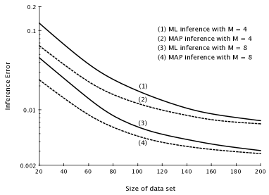
(a) Effect of Observation Duration

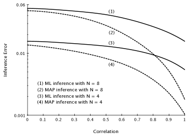
(b) Effect of Spatial Correlation of Sensing Values

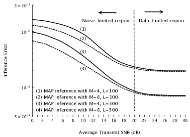
(c) Effect of Average Transmit SNR

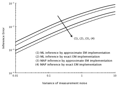
(d) Effect of Measurement Noise

Figure 5: The effects of system parameters on the accuracy of reader’s statistical inference.

VI-B Effect of Spatial Correlation of Sensing Values

The impact of the correlation coefficient $\rho$ on the inference accuracy is evaluated in Fig. 5(b). The measurement noise is assumed negligible, and we set $M=4$ and $L=100$. One can observe from the curves that spatial correlation between sensing values helps reader inference by improving its accuracy. In particular, MAP inference sees a much more significant performance improvement compared with the ML counterpart as $\rho$ increases. The reason is that the correlation information is explicitly encoded in the prior distribution and exploited by the MAP inference but not ML. In other words, the accessibility of the prior distribution of the environment variables plays a critical role in determining how much gain can be exploited from the spatial correlation between them. The above observation hold for different $N$ settings. However, increasing $N$ leads to a decline in decoding accuracy as the number of unknown to be inferred by the reader grows.

VI-C Effect of Average Transmit SNR

Fig. 5(c) displays the curves of inference error versus the average transmit SNR for different values of $M$ and $L$. The figure only shows the curves for MAP inference without measurement noise. Simulation results for other cases (e.g., ML inference and the presence of measurement noise) are omitted as they all show similar trends. One can observe that as the SNR increases, the inference error sees fast decrease in the low-to-moderate SNR regime. However when the SNR is large (exceeds about $20$ dB), the accuracy cannot be further improved by simply increasing the transmission power. The reason is that in the high SNR regime the bottleneck of accurate inference is no longer the noise but the data-set size. Increasing the size (or equivalently the observation duration) can lower the error-saturation level. Furthermore, it is also noted that increasing the number of receive antenna $M$ can considerably alleviate the distortion from noise when SNR is low due to the said diversity gain, but still suffer from the same error floor in the high SNR regime.

VI-D Tightness of Variational-Inference Approximation

Consider the scenario with presence of measurement noise, resulting in the dimensionality of the latent space linearly growing with the number of sensors. The performance of the exact EM implementation is compared with its approximate implementation by variational inference in Fig. 5(d) over varying the variance of measurement noise. It is observed that, for both the cases of ML and MAP inference, the approximation leads to only a marginal performance loss compared with exact EM but leads to reduced computation complexity. This confirms the effectiveness of variational inference. Moreover, one can also observe that the inference performance is satisfactory even in the regime of strong measurement noise (e.g., the error is less than $0.1$ when $\delta^{2}=10$). This shows the robustness of reader inference against the corruption of measurement noise.

VII Concluding Remarks

The work presents a novel design framework for backscatter sensor systems. The design features the application of machine learning to tackle hardware and signal processing limitations of backscatter sensors as well as reducing overhead (due to e.g., scheduling protocol and channel estimation and feedback). This work represents an initial investigation of a promising approach of leveraging powerful techniques from machine learning to implement intelligent sensor networks. There are many interesting directions warranting further research. For instance, for large-scale networks with mobile readers (e.g., for Smart Cities), machine learning can be applied to jointly design reader inference and path planning. As another example, inference from large-scale sensing data can be centralized in the cloud using advanced machine learning such as deep learning. Alternatively, a hierarchical framework can be developed for data inference combining centralized and distributed inference. All such interesting directions call for novel designs integrating machine learning and wireless communications in the same vein as the current work but in potentially more complex ways.

-A Proof of Lemma 1

Starting from the cumulative distribution function (CDF) of $\boldsymbol{\theta}$, denoted by $F_{\boldsymbol{\theta}}({\mathbf{u}})$, by definition and the mapping function shown in (5) we have

$$F_{\boldsymbol{\theta}}({\mathbf{u}}) =\text{Prob}\left(\frac{1}{1+\exp\left(-\frac{x_{1}-\mu_{1}}{\sigma_{1}}\right)}<u_{1},\cdots,\frac{1}{1+\exp\left(-\frac{x_{N}-\mu_{N}}{\sigma_{N}}\right)}<u_{N}\right)$$

$$=\text{Prob}\left(x_{1}<-\sigma_{1}\log\left(\frac{1}{u_{1}}-1\right)+\mu_{1},\cdots,x_{N}<-\sigma_{N}\log\left(\frac{1}{u_{N}}-1\right)+\mu_{N}\right)$$

$$=F_{{\mathbf{x}}}\left(-\sigma_{1}\log\left(\frac{1}{u_{1}}-1\right)+\mu_{1},\cdots,-\sigma_{N}\log\left(\frac{1}{u_{N}}-1\right)+\mu_{N}\right),$$ (53)

in which $F_{{\mathbf{x}}}(\cdot)$ represent the CDF of ${\mathbf{x}}$. Then the PDF of $\boldsymbol{\theta}$ can be evaluated by taking derivative of (-A) with respect to ${\mathbf{u}}=[u_{1},u_{2},\cdots,u_{N}]^{T}$, namely

$$p(\boldsymbol{\theta}) =\left.\frac{\partial}{\partial{\mathbf{u}}}F_{{\mathbf{x}}}\left(-\sigma_{1}\log\left(\frac{1}{u_{1}}-1\right)+\mu_{1},\cdots,-\sigma_{N}\log\left(\frac{1}{u_{N}}-1\right)+\mu_{N}\right)\right|_{{\mathbf{u}}=\boldsymbol{\theta}}$$

$$=\prod_{n=1}^{N}\frac{\sigma_{n}}{\theta_{n}-\theta_{n}^{2}}f_{{\mathbf{x}}}\left(-\sigma_{1}\log\left(\frac{1}{\theta_{1}}-1\right)+\mu_{1},\cdots,-\sigma_{N}\log\left(\frac{1}{\theta_{N}}-1\right)+\mu_{N}\right),$$ (54)

where $f_{{\mathbf{x}}}(\cdot)=p({\mathbf{x}})$ denotes the PDF of ${\mathbf{x}}$ as given by (2). Then the desired result can be obtained by substituting (2) into (-A), completing the proof.

-B Proof of Proposition 1.A

Let $\tilde{\cal L}(\theta)$ denote the objective function shown in (24), then the first and second derivatives of $\tilde{\cal L}(\theta)$ with respect to $\theta$ can be expressed as follows

$$\tilde{\cal L}^{\prime}(\theta) =\sum_{i=1}^{L}\sum_{m=0}^{N}q^{(i)}_{T}(m)\left(\frac{m}{\theta}-\frac{N-m}{1-\theta}\right).$$ (55)

$$\tilde{\cal L}^{\prime\prime}(\theta) =-\sum_{i=1}^{L}\sum_{m=0}^{N}q^{(i)}_{T}(m)\left(\frac{m}{\theta^{2}}+\frac{N-m}{(1-\theta)^{2}}\right).$$ (56)

Note that $q^{(i)}_{T}(m)$ is non-negative as it is a probability measure, hence it is easy to see that $\tilde{\cal L}^{\prime\prime}(\theta)<0,\;\;\forall\theta\in(0,1)$, suggesting $\tilde{\cal L}(\theta)$ is a concave function over its domain $\theta\in(0,1)$. As a result, the maximum of $\tilde{\cal L}(\theta)$ can be achieved by setting its first derivative to zero, leading to the desired result in (25). However, one should take note that the zero of $\tilde{\cal L}^{\prime}(\theta)$ may not lie in the range of $(0,1)$, thereby requiring further validation of the solution. Fortunately, the result shown in (25) is guaranteed to meet the constraint $\theta\in(0,1)$. To see this, let’s rewrite (25) as $\theta^{*}=\frac{1}{L}\sum_{i=1}^{L}\left(\frac{1}{N}\sum_{m=0}^{N}q^{(i)}_{T}(m)m\right)$. Note that the term inside the bracket can be identified as the expectation of $T^{(i)}$ with respect to its posterior distribution $q^{(i)}$ normalized by its maximum value $N$ which should fall in the range $(0,1)$ for each $i$. Hence a further average over $i$ still keeps the value within $(0,1)$, which completes the proof.

-C Proof of Proposition 1.B

Denoting $\tilde{\cal L}(\Sigma_{m})$ as the objective function shown in (27). Then taking the first and second derivatives of $\tilde{\cal L}(\Sigma_{m})$ with respect to $\Sigma_{m}$ gives

$$\nabla_{\Sigma_{m}}\tilde{\cal L}(\Sigma_{m})=\sum_{i=1}^{L}q^{(i)}_{T}(m)\left(-\frac{M}{\Sigma_{m}}-\frac{\|{\mathbf{y}}^{(i)}\|^{2}}{2\Sigma_{m}^{2}}\right).$$ (57)

$$\nabla^{2}_{\Sigma_{m}}\tilde{\cal L}(\Sigma_{m})=-\sum_{i=1}^{L}q^{(i)}_{T}(m)\left(\frac{M\Sigma_{m}-\|{\mathbf{y}}^{(i)}\|^{2}}{\Sigma_{m}^{3}}\right)=\frac{\Sigma_{m}-\frac{\sum_{i=1}^{L}q^{(i)}_{T}(m)\|{{\mathbf{y}}^{(i)}}\|_{2}^{2}}{M\sum_{i=1}^{L}q^{(i)}_{T}(m)}}{\Sigma_{m}^{3}/(M\sum_{i=1}^{L}q^{(i)}_{T}(m))}.$$ (58)

Although $\nabla^{2}_{\Sigma_{m}}\tilde{\cal L}(\Sigma_{m})$ is not non-positive for all $\Sigma_{m}\in\mathbb{R^{+}}$, in other words, $\tilde{\cal L}(\Sigma_{m})$ is not a concave function on its domain $\Sigma_{m}\in\mathbb{R}$, we can still prove that the maximum of $\tilde{\cal L}(\Sigma_{m})$ is attained at the zero of its first derivative due to its quasi-concavity as shown below. Particularly, note that there is only one root for $\nabla_{\Sigma_{m}}\tilde{\cal L}(\Sigma_{m})=0$, namely $\Sigma_{m}^{*}$ derived in (28). Furthermore, as can be seen from (58) that the second derivative at that critical point is strictly less than zero, i.e., $\nabla^{2}_{\Sigma_{m}}\tilde{\cal L}(\Sigma_{m}^{*})<0$. The above observations plus the fact that $\tilde{\cal L}(\Sigma_{m})$ is a continuous function and differentiable everywhere on its domain $\Sigma_{m}>0$ lead to the desired result.

References

- [1] C. Boyer and S. Roy, “Backscatter communication and RFID: Coding, energy, and MIMO analysis,” IEEE Trans. Commun., vol. 62, no. 3, pp. 770–785, Mar. 2014.
- [2] G. Yang, C. K. Ho, and Y. L. Guan, “Multi-antenna wireless energy transfer for backscatter communication systems,” IEEE J. Sel. Areas Commun., vol. 33, no. 12, pp. 2974–2987, Dec. 2015.
- [3] J. Kimionis, A. Bletsas, and J. N. Sahalos, “Increased range bistatic scatter radio,” IEEE Trans. Commun., vol. 62, no. 3, pp. 1091–1104, Mar. 2014.
- [4] B. Clerckx, Z. B. Zawawi, and K. Huang, “Wirelessly powered backscatter communications: Waveform design and snr-energy tradeoff,” to appear in IEEE Commun. Lett.
- [5] J. Qian, F. Gao, G. Wang, S. Jin, and H. Zhu, “Noncoherent detections for ambient backscatter system,” IEEE Trans. Wireless Commun., vol. 16, no. 3, pp. 1412–1422, Mar. 2017.
- [6] P. N. Alevizos, A. Bletsas, and G. N. Karystinos, “Noncoherent short packet detection and decoding for scatter radio sensor networking,” IEEE Trans. Commun., vol. 65, no. 5, pp. 2128–2140, May 2017.
- [7] W. Liu, K. Huang, X. Zhou, and S. Durrani, “Full-duplex backscatter interference networks based on time-hopping spread spectrum,” IEEE Trans. Wireless Commun., vol. 16, no. 7, pp. 4361–4377, Jul. 2017.
- [8] K. Han and K. Huang, “Wirelessly powered backscatter communication networks: Modeling, coverage, and capacity,” IEEE Trans. Wireless Commun., vol. 16, no. 4, pp. 2548–2561, Apr. 2017.
- [9] B. Zhen, M. Kobayashi, and M. Shimizu, “Framed ALOHA for multiple RFID objects identification,” IEICE Trans. Commun., vol. E88-B, no. 3, pp. 991–999, Mar. 2005.
- [10] M. T. Isik and O. B. Akan, “PADRE: Modulated backscattering-based passive data retrieval in wireless sensor networks,” in Proc. IEEE Wireless Commun. Networking Conf. (WCNC), Budapest, Hungary, Apr. 2009, pp. 1–6.
- [11] Y. Zheng, M. Li, Y. Zheng, and M. Li, “Read bulk data from computational RFIDs,” IEEE/ACM Trans. Netw., vol. 24, no. 5, pp. 3098–3108, Oct. 2016.
- [12] D. T. Hoang, D. Niyato, P. Wang, D. I. Kim, and L. B. Le, “Optimal data scheduling and admission control for backscatter sensor networks,” IEEE Trans. Commun., vol. 65, no. 5, pp. 2062–2077, May 2017.
- [13] C. Angerer, R. Langwieser, and M. Rupp, “RFID reader receivers for physical layer collision recovery,” IEEE Trans. Commun., vol. 58, no. 12, pp. 3526–3537, Dec. 2010.
- [14] S. Kim, S. Kwack, S. Choi, and B. G. Lee, “Enhanced collision arbitration protocol utilizing multiple antennas in RFID systems,” in Proc. 17th Asia Pacific Conf. on Commun., Sabah, Malaysia, Oct. 2011, pp. 925–929.
- [15] T. Demeechai and S. Siwamogsatham, “Using CDMA to enhance the MAC performance of ISO/IEC 18000-6 Type C,” IEEE Commun. Lett., vol. 15, no. 10, pp. 1129–1131, Oct. 2011.
- [16] J. Wang, H. Hassanieh, D. Katabi, and P. Indyk, “Efficient and reliable low-power backscatter networks,” in Proc. ACM SIGCOMM, Helsinki, Finland, Aug. 2012, pp. 61–72.
- [17] J. Chen, U. Yatnalli, and D. Gesbert, “Learning radio maps for UAV-aided wireless networks: A segmented regression approach,” in Proc. IEEE Int. Conf. Commun. (ICC), Paris, France, May 2017.
- [18] N. Farsad and A. Goldsmith, “Detection algorithms for communication systems using deep learning,” arXiv preprint arXiv:1705.08044, 2017.
- [19] J. Barbancho, C. León, F. J. Molina, and A. Barbancho, “A new QoS routing algorithm based on self-organizing maps for wireless sensor networks,” Telecommun. Syst.,, vol. 36, no. 1-3, pp. 73–83, Mov. 2007.
- [20] B. Krishnamachari and S. Iyengar, “Distributed Bayesian algorithms for fault-tolerant event region detection in wireless sensor networks,” IEEE Trans. Comput., vol. 53, no. 3, pp. 241–250, Mar. 2004.
- [21] M. R. Morelande, B. Moran, and M. Brazil, “Bayesian node localisation in wireless sensor networks,” in Proc. IEEE Int. Conf. Acousti., Speech Signal Process., Mar. 2008, pp. 2545–2548.
- [22] J. Kho, A. Rogers, and N. R. Jennings, “Decentralized control of adaptive sampling in wireless sensor networks,” ACM Trans. Sen. Netw., vol. 5, no. 3, pp. 19:1–19:35, May 2009.
- [23] G. Mergen and L. Tong, “Type based estimation over multiaccess channels,” IEEE Trans. on Signal Process., vol. 54, no. 2, pp. 613–626, Feb. 2006.
- [24] B. Chen, L. Tong, and P. K. Varshney, “Channel-aware distributed detection in wireless sensor networks,” IEEE Signal Processing Mag., vol. 23, no. 4, pp. 16–26, Jul. 2006.
- [25] I. Glaropoulos, M. Laganà, V. Fodor, and C. Petrioli, “Energy efficient COGnitive-MAC for sensor networks under WLAN co-existence,” IEEE Trans. Wireless Commun., vol. 14, no. 7, pp. 4075–4089, Jul. 2015.
- [26] Z. Liu and I. Elhanany, “RL-MAC: a reinforcement learning based mac protocol for wireless sensor networks,” International Journal of Sensor Networks, vol. 1, no. 3-4, pp. 117–124, 2006.
- [27] Y.-J. Shen and M.-S. Wang, “Broadcast scheduling in wireless sensor networks using fuzzy Hopfield neural network,” Expert systems with applications, vol. 34, no. 2, pp. 900–907, 2008.
- [28] M. J. Beal, Variational algorithms for approximate Bayesian inference. University of London United Kingdom, 2003.
- [29] W. Che, H. Deng, W. Tan, and J. Wang, “A random number generator for application in RFID tags,” in Networked RFID Systems and Lightweight Cryptography. Springer Berlin Heidelberg, 2008, pp. 279–287.
- [30] G. K. Balachandran and R. E. Barnett, “A 440-nA true random number generator for passive RFID tags,” IEEE Trans. Circuits Syst. I, Reg. Papers, vol. 55, no. 11, pp. 3723–3732, Dec. 2008.
- [31] M. Fernández and S. Williams, “Closed-form expression for the poisson-binomial probability density function,” IEEE Trans. Aerosp. Electron. Syst., vol. 46, no. 2, pp. 803–817, Apr. 2010.
- [32] M. R. Gupta and Y. Chen, “Theory and use of the EM algorithm,” Foundations and Trends® in Signal Processing, vol. 4, no. 3, pp. 223–296, 2011.
- [33] K. P. Murphy, Machine learning: a probabilistic perspective. MIT press, 2012.
- [34] R. M. Neal and G. E. Hinton, “A view of the EM algorithm that justifies incremental, sparse, and other variants,” in Learning in graphical models. Springer, 1998, pp. 355–368.
- [35] L. P. Kadanoff, “More is the same; phase transitions and mean field theories,” Journal of Statistical Physics, vol. 137, no. 5-6, pp. 777–797, 2009.
- [36] S. L. Simpson, L. J. Edwards, K. E. Muller, P. K. Sen, and M. A. Styner, “A linear exponent AR (1) family of correlation structures,” Statistics in medicine, vol. 29, no. 17, pp. 1825–1838, 2010.