Congestion Barcodes: Exploring the Topology of Urban Congestion Using Persistent Homology

Abstract.

This work presents a new method to quantify connectivity in transportation networks. Inspired by the field of topological data analysis, we propose a novel approach to explore the robustness of road network connectivity in the presence of congestion on the roadway. The robustness of the pattern is summarized in a congestion barcode, which can be constructed directly from traffic datasets commonly used for navigation. As an initial demonstration, we illustrate the main technique on a publicly available traffic dataset in a neighborhood in New York City.

1. Introduction

1.1. Motivation

Not only are today’s cities challenged with an excess of congestion, they now are faced with an array of routing algorithms, apps, and other tools which can easily lead to unexpected and emergent behaviors. On the other hand, with more data now available, it is becoming possible to think of big-data approaches to understanding large-scale mobility problems and compare cities  [1, 2, 3, 4, 5, 6].

Our effort here is to understand the topology of congestion. Road infrastructure, passenger travel demands, and real-time information systems all can interact to create complex behaviors on road networks. An important analytical challenge is to construct coarse (e.g., low dimensional) descriptions of the transportation system from the high dimensional datasets, from which one can then draw conclusions and make data driven decisions. Our interest is to apply some recent characterizations of general networks to understand large-scale behaviors, with the hope it will eventually support new ways to understand and compare mobility behaviors.

1.2. Problem statement and related work

The focus of the present work is to uncover the topology of traffic congestion. This is relevant in addressing questions about its spatial variability. For example, trips between OD regions might pass through congested road segments, or multiple “islands” of smooth flowing traffic might exist in the interior of a set of congested links. More broadly, the interrelationship between congestion and connectedness can lead to traffic frustration, emergent behaviors, and exacerbated gridlock, and we consequently seek methods to quantify this structure.

Our interest here is applying topological data analysis to traffic behavior and predictability. To facilitate new approaches to address urban traffic, cities (viz. Chicago [7] and New York City [8]) are releasing large mobility datasets. We believe that this line of inquiry may give some new types of useful insights which “coarse-grain” behaviors in such a way that we can seek to compare cities and transfer quantitative knowledge from one place to another.

A variety of topological information can be studied. The simplest “homology” counts the number of connected components in the topology. One can also construct homologies reflecting the structure of paths; this has implications for robotic path planning in the face of uncertainty [9] and also connectivity in the brain [10]. By way of precedence, the article [11], uses persistent homology to measure similarities between road maps.

Persistent homology, introduced by [12] and [13], (see also [13, 14, 9, 15]) seeks to “unfold” geometries of datasets, giving new insights into the structure of the data and the robustness of this structure. Many datasets naturally have an unfolding parameter, and one can compute how various topological objects (characterized as null spaces, ranges, and other linear-algebraic objects) appear and disappear as the parameter changes. Topological objects which persist over large ranges of parameter values can be interpreted as stable and robust, while those which are short-lived in parameter space might be thought of as noise. A barcode, described in detail later, allows one to graphically capture dependence on parameters.

When applied to traffic networks, these techniques can help us analyze large travel datasets and generate useful insights. In particular, it provides a way to capture the relationships between the following aspects of a transportation network with respect to a given speed threshold: number of connected links that meet such threshold, sizes of such connected links, and coverage of the region given a speed thresholds.

The original motivation for persistent homology was in understanding stable aspects of point clouds of data (see [16]). In that case, a distance parameter $\varepsilon$ can be used to connect points (the Čech or Rips complexes). As the parameter $\varepsilon$ is increased, more points are included in the simplices; understanding the robust aspect of these simplices allows one to reconstruct the essential features of the point cloud in ways which are somewhat impervious to noise. This has been adapted to image processing [17] and analysis of coverage of sensor networks [18], and the structure of some data in global development [19]. Persistence of more complicated geometric invariants have been used to study feasibility sets in robotics; see [20].

1.3. Outline and contributions

The main contribution of this work is the application of persistent homology to understanding road traffic networks. To our knowledge, this is the first application of topological data analysis to traffic. Our hope is that this line of research will lead to some new and robust techniques of capturing the structure of congestion in ways which can be used to compare different cities and regions.

In Section  2, we provide a brief introduction of persistent homology and explain how it is applied to road networks. In Section 3, we provide the algorithms used to construct a ”congestion barcode”, before applying it in Section 4 to a small example from New York City.

2. Background on Persistent Homology

We briefly review the main ideas of persistent homology and explain how it can be applied to road networks. The interested reader is referred to [15, 16] for a detailed description and survey of applications. We develop the notion of persistence for the simplest invariant; the number of connected components (corresponding to the zero-th Betti number; see [21]). We will here develop the notion of connectedness as, informally, a set of good (e.g., fast) roads, all of which one can traverse without ever needing to drive on a bad (slow) road.

Abstractly, we have a weighted undirected finite graph $G=(V,E)$ where $V$ is a finite set of vertices, which we interpret as intersections, and $E$ is the set of edges, which we interpret as roads or links. Each edge $e$ is a set $\{v_{1},v_{2}\}$ of two distinct vertices; $e$ connects $v_{1}$ and $v_{2}$. Each edge $e$ has a nonnegative weight $W_{e}$. For specificity, we will think of the weights as speeds, so higher weights correspond to better traffic conditions. For simplicity, we assume that each $v\in V$ is in one of the edges $e\in E$ (i.e., $G$ has no disconnected vertices).

If $G^{\prime}=(V^{\prime},E^{\prime})$ is a finite graph, we say that a subset $C\subset V^{\prime}$ is connected if, for every pair $v^{\prime}_{a}$ and $v^{\prime}_{b}$ of vertices in $C$, there is a sequence $\{v^{\prime}_{n}\}_{n=1}^{N}$ of vertices with $v^{\prime}_{1}=v^{\prime}_{a}$ and $v^{\prime}_{N}=v^{\prime}_{b}$, such that $\{v^{\prime}_{n},v^{\prime}_{n+1}\}\in E^{\prime}$; i.e., there is a path leading from $v^{\prime}_{a}$ to $v^{\prime}_{b}$ along the edges in $E^{\prime}$. We can decompose $V^{\prime}$ into a finite collection of maximal connected components.

We finally introduce a concept of a level, or persistence parameter, which is used to construct and compare subgraphs. For each level $\lambda\in[0,\infty)$, define a subgraph $G(\lambda)$ generated by edges whose weight is greater than $\lambda$ as

(1) $$G(\lambda)\overset{\text{def}}{=}(V_{\lambda},E_{\lambda}),$$

where

(2) $$E_{\lambda}=\{e\in E:W_{e}>\lambda\},$$

and where

(3) $$V_{\lambda}=\bigcup_{e\in E_{\lambda}}e.$$

2.1. Barcodes explained

The focus of persistent homology is understanding how the topology of $G(\lambda)$ changes as $\lambda$ changes. To start, we note that

$$G(\lambda_{1})\subset G(\lambda_{2})$$

if $\lambda_{1}\geq\lambda_{2}$ (i.e., $V_{\lambda_{1}}\subset V_{\lambda_{2}}$ and $E_{\lambda_{1}}\subset E_{\lambda_{2}}$). Intuitively, as $\lambda$ decreases, we include more links in the definition of $E_{\lambda}$ (and thus $V_{\lambda}$). The map $\lambda\mapsto G(\lambda)$ is a reverse filtration (the $G(\lambda)$’s get larger as $\lambda$ decrease, as opposed to getting larger as $\lambda$ increases).

Our goal here is to understand how the connected components of $G(\lambda)$ change as $\lambda$ decreases and $G(\lambda)$ fills in more and more of $G$. Informally, we think of the parameter $\lambda$ as reversed time (we want to use reversed time, since connected components appear as the “time” parameter $\lambda$ decreases). For $\lambda_{1}$ and $\lambda_{2}$ with $\lambda_{1}>\lambda_{2}$, we want to compare the connected components of $G(\lambda_{1})$ with those of $G(\lambda_{2})$. Several things can happen. $G(\lambda_{2})$ can contain a new connected component (a “birth”). Connected components can merge and some of them will “die”. Finally, a connected component can grow in size without merging with other connected components.

A barcode focuses on the evolution the connected components of $G(\lambda)$ by mapping each connected component into a different line, or bar. A bar starts when the corresponding component is born, and ends when it merges (the bar reflects the growth of a connected component as long as it does not merge). The structure of the different bars will help us visualize how connected components of the good parts of the traffic network appear and merge.

We can think of each bar in the barcode as a key-value dictionary which evolves with the parameter $\lambda$. The bar consists of a start value when the barcode was born, an end value when the bar merged and died (if it has in fact already merged), and a state consisting of the current connected component. The state of the bar keeps the information we need to compare the current (i.e., the current value of $\lambda$) connected set to a connected set at a later time. The barcode is a list of bars.

Focusing on the death of bars, we need to agree on which bar to extend when two connected components merge. When bars merge, we say that the oldest bar–i.e., the one with the highest start value (recall that we are reversing time, so “older” means larger starting values)–survives, while the younger ones (the ones with lower starting value) die.

We define the persistence of each bar as the absolute difference between its start and end $\lambda$-values. We represent these bars in a plot with the length of each bar being proportional to its persistence, ordering the bars by total length with the longest bars on the bottom. we call this plot the barcode diagram, or simply the barcode.

If a component exists for wide range of levels $\lambda$ i.e. its bar has a high persistence, we can think of it as robust; if a component exists only for a short range of parameter values, one might interpret it as result of noise.

3. Algorithm

The first step is to decompose each $G(\lambda)$ into connected components. A depth-first search  [22] can efficiently do this; see Algorithm 1.

Algorithm 1 Create list of connected components of $G(\lambda)$ using depth first search

1:Label all vertices in $V_{\lambda}$ as “unvisited”$\triangleright$ We relabel the vertices as they appear in connected subsets of $G(\lambda)$

2:Let $\mathcal{W}$ be a list of connected components of $G(\lambda)$$\triangleright$ Initially empty

3:for each vertex $v\in V_{\lambda}$ which is still “unvisited” do

4:     Start a new connected component $C$ which contains (is “rooted” at) $v$ $\triangleright$ $C=\{v\}$

5:     function DFS(node v’) $\triangleright$ Define recursive function which adds new vertices to $C$ and “visits” vertices

6:         for each unvisited vertex $v^{\prime\prime}\in V_{\lambda}$ with $W_{v^{\prime},v^{\prime\prime}}>\lambda$ do $\triangleright$ $v^{\prime\prime}$ is connected to $v^{\prime}$ in $G(\lambda)$

7:              label $v^{\prime\prime}$ as visited

8:              add $v^{\prime\prime}$ to $C$

9:              DFS($v^{\prime\prime}$)$\triangleright$ Recursive step

10:         end for

11:     end function$\triangleright$ DFS has modified $C$ and ”visited” vertices

12:      DFS(v)$\triangleright$ Apply DFS to $v$

13:     Add $C$ to $\mathcal{W}$ $\triangleright$ $C$ is the unique connected component of $G(\lambda)$ which contains $v$

14:end for

This gives us the connected components of $G(\lambda)$. We visit each vertex in $V(\lambda)$ and recursively find the other vertices which are connected by a weight of more than $\lambda$.

One of the computational challenges of constructing barcodes is efficiently carrying out the comparisons between the components of the current $G(\lambda)$, which we compute via the depth-first search algorithm, and the state values (i.e., connected sets) of the bars at the prior values. Note that the $G(\lambda)$’s (and thus their connected components) only change at the different values of

(4) $$\Lambda\overset{\text{def}}{=}\{W_{e}:e\in E\}.$$

To facilitate merging, let’s organize the list of bars in the barcode by start time, with larger start time (i.e., older age) being first. The merging order outlined in Subsection 2.1 thus corresponds to the bars with the higher list index merging into the one with the lower list index. We carry this out in Algorithm 2; when a bar b dies, we cease updating its end value. To aid in the clarity of the merging process, we could also, in Algorithm 2 set the state of a dead bar to $\emptyset$.

Algorithm 2 Create barcodes. A bar b is a key-value dictionary consisting of a start, end, and state.

1:Create ordered list $B$ of bars$\triangleright$ Initially empty.

2:for each $\lambda\in\Lambda$ of (4), ordered by decreasing value do$\triangleright$ Reverse time

3:     for each connected component $C$ of $G(\lambda)$ do$\triangleright$ Use DFS

4:         for each barcode $b\in B$, with oldest bars first do

5:              if $C$ and b[state] intersect then

6:                  if we have not yet declared a merge then

7:                       Declare a merge$\triangleright$ Occurs for oldest intersecting bar; extend this bar

8:                       b[end]$\leftarrow\lambda$$\triangleright$ extend bar to at least current time

9:                       b[state]$\leftarrow C$

10:                  else$\triangleright$ $C$ intersects with younger bar

11:                       bar dies

12:                  end if

13:              end if

14:         end for

15:         if a merge has not yet been declared then$\triangleright$ $C$ has not intersected with any bar

16:              start a new bar with start set to $\lambda$ and state set to $C$.

17:         end if

18:     end for

19:end for

Each connected component can merge several bars, extending only one of them (the oldest). Since $\lambda\mapsto G(\lambda)$ is a reverse filtration (i.e., $\lambda\mapsto G(\lambda)$ is decreasing in $\lambda$), different connected components of $G(\lambda)$ cannot affect the same bar.

4. Description of the dataset: New York City traffic speeds

We are interested in developing our ideas for a restricted dataset. We start with a dataset of 2011 taxi data [8] as processed by [23] and look at traffic speeds in the Diamond district between 9 and 10 AM on workdays during June, July and August of 2011. Roughly, this dataset should reflect traffic behavior which is fairly homogeneous in time, allowing us to focus on spatial fluctuations. The roads are highlighted in Figure 1. We consider $152$ one-directional links, corresponding to 144 roads; there are 8 two-way roads. The dataset has $D\overset{\text{def}}{=}66$ days in it.

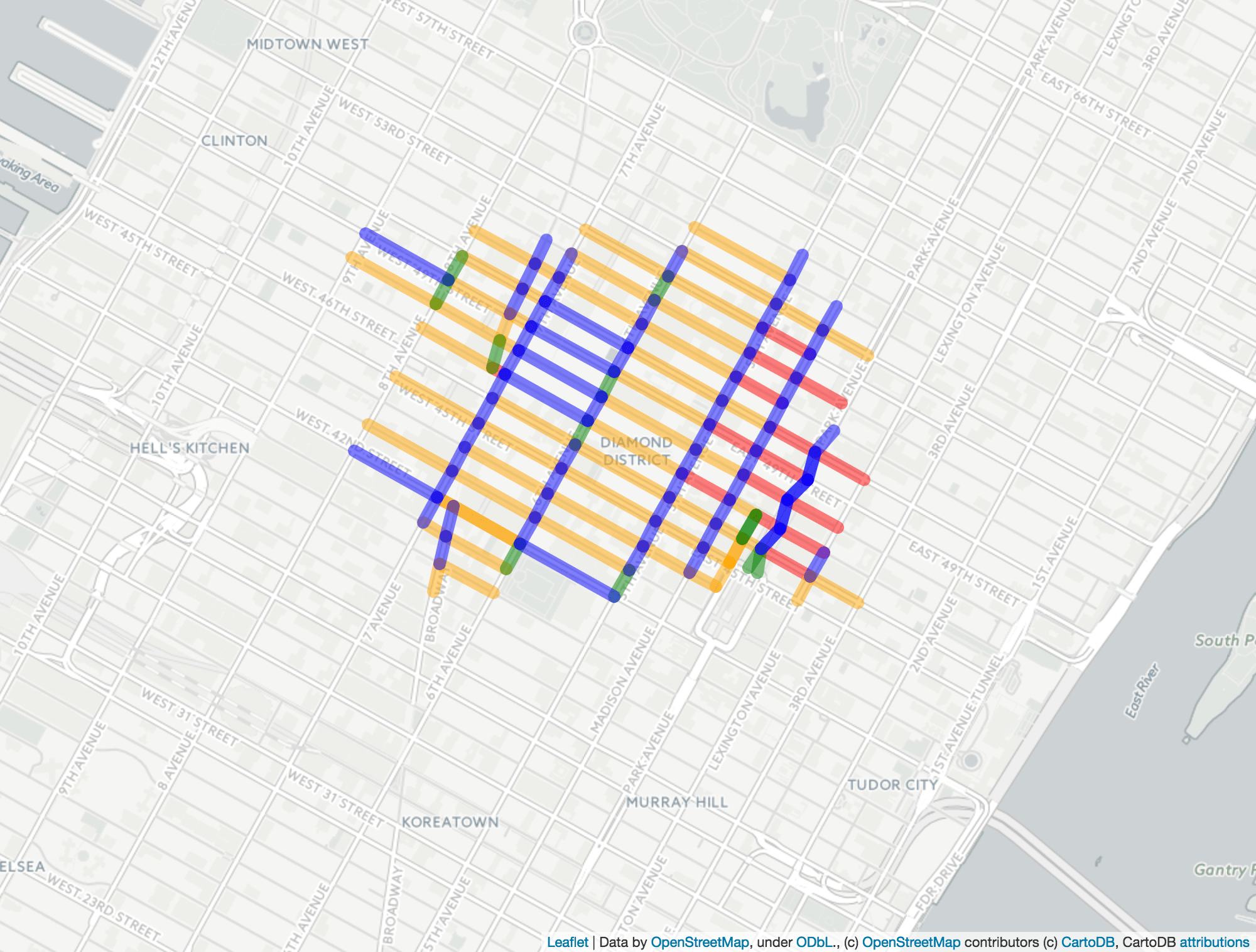
Figure 1. Case study network. Diamond District streets (144 links, and 74 nodes) in New York City. The red roads correspond to speeds in $[0,2)$, the orange roads correspond to speeds in $[2,3)$, the blue roads correspond to speeds in $[3,4)$, and the green roads correspond to speeds in $[4,\infty)$.

If we let $s_{\ell,t}$ correspond to the speed in link $\ell$ on day $t$, let’s define

(5) $$W_{\ell}\overset{\text{def}}{=}\frac{1}{D}\sum_{d=1}^{D}s_{\ell,t}$$

as the average speed on link $\ell$. To resolve the ambiguity of this definition on the $8$ two-way roads, we replace (5) by the average over both directions during this time; we average over the $132$ speeds corresponding to $66$ speeds in one direction, and $66$ speeds in the other. This affects only 8 roads, and reflects a somewhat justifiable assumption that congestion in one direction may cause congestion, both by proximity and by left turns.

The $S_{\ell}$’s, the average speeds on the different links, range from 1.5 m/s to 5.00 m/s (all speeds are in meters/second), with average of 3.0 m/s and standard deviation of 0.78 m/s. The low speeds come from the fact that the area is highly congested in the late morning hour from which the data was obtained. See Figure 2 for a histogram of the speed distribution on the graph.

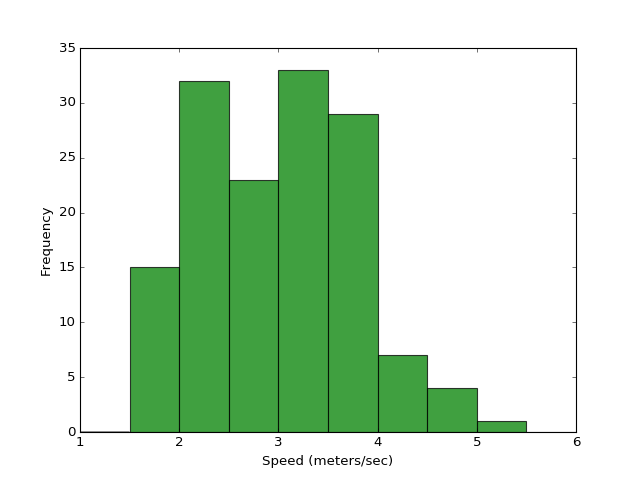
Figure 2. Histogram of the average road speed in the Diamond District from 9-10 AM in the summer of 2011.

We are primarily interested in how these speeds are spatially distributed. In Figure 3(a), the streets with speeds greater than 4.0 m/s are highlighted in red; these are the fastest streets. In Figure 3(b), the streets with speeds between 3.5 and 4 m/s are highlighted; these are slightly slower. Figure 3(f) gives roads with speeds less than 2, while Figure 3(e) gives roads with speeds between 2 and 2.5; these are the slowest and second-slowest roads.

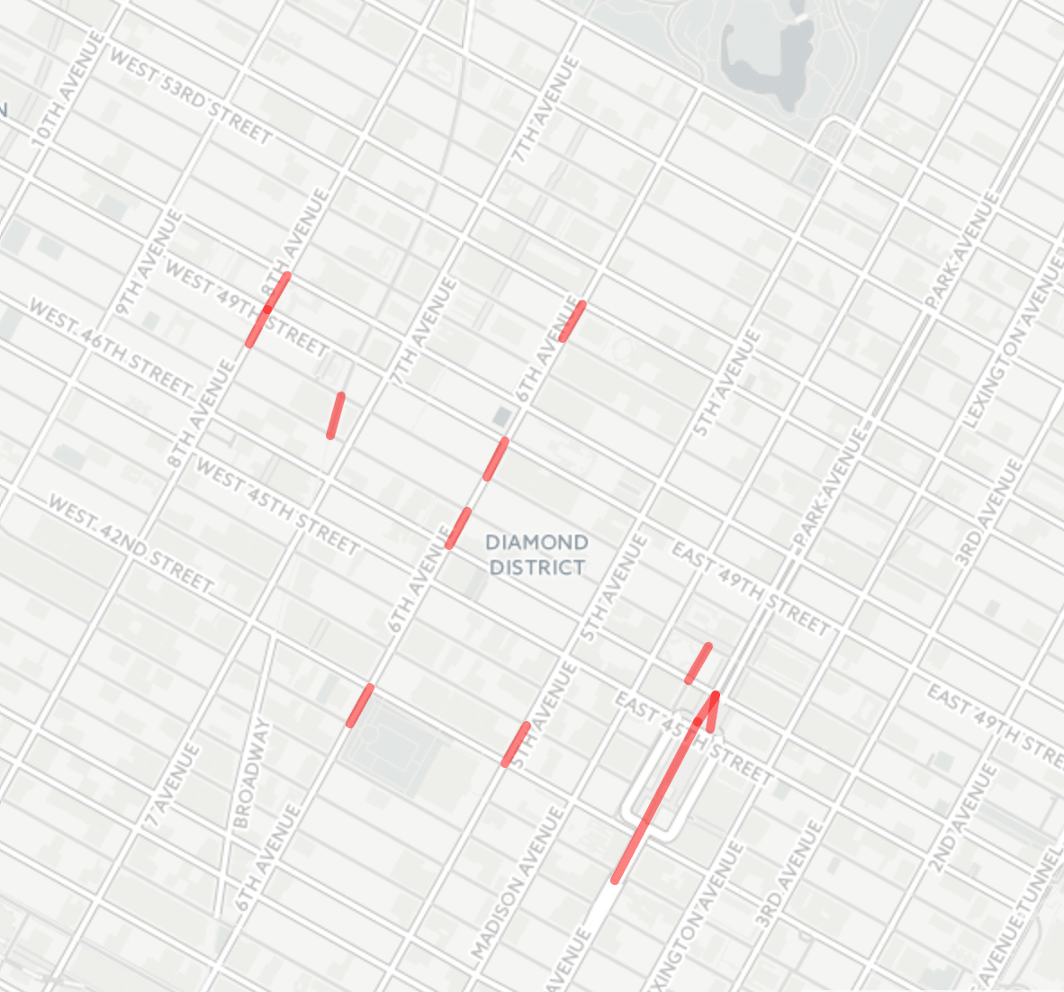
(a) Roads with speeds in $[4,\infty)$.

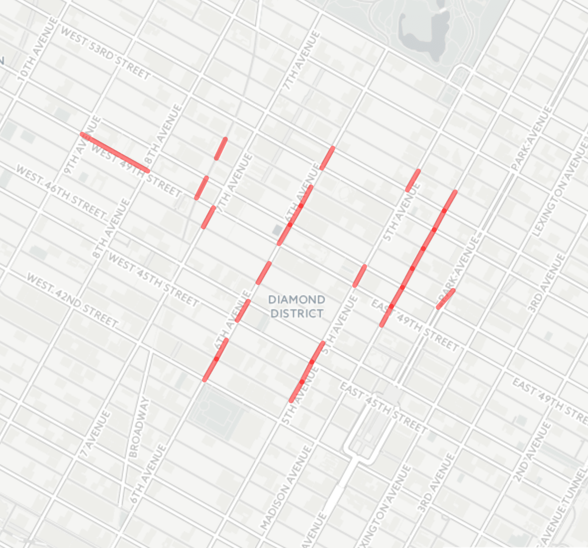
(b) Roads with speeds in $[3.5,4)$.

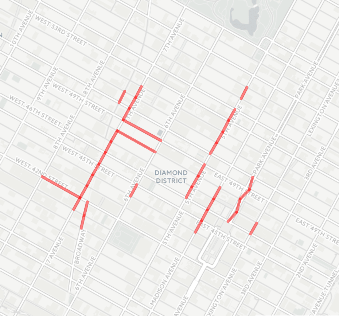
(c) Roads with speeds in $[3,3.5)$.

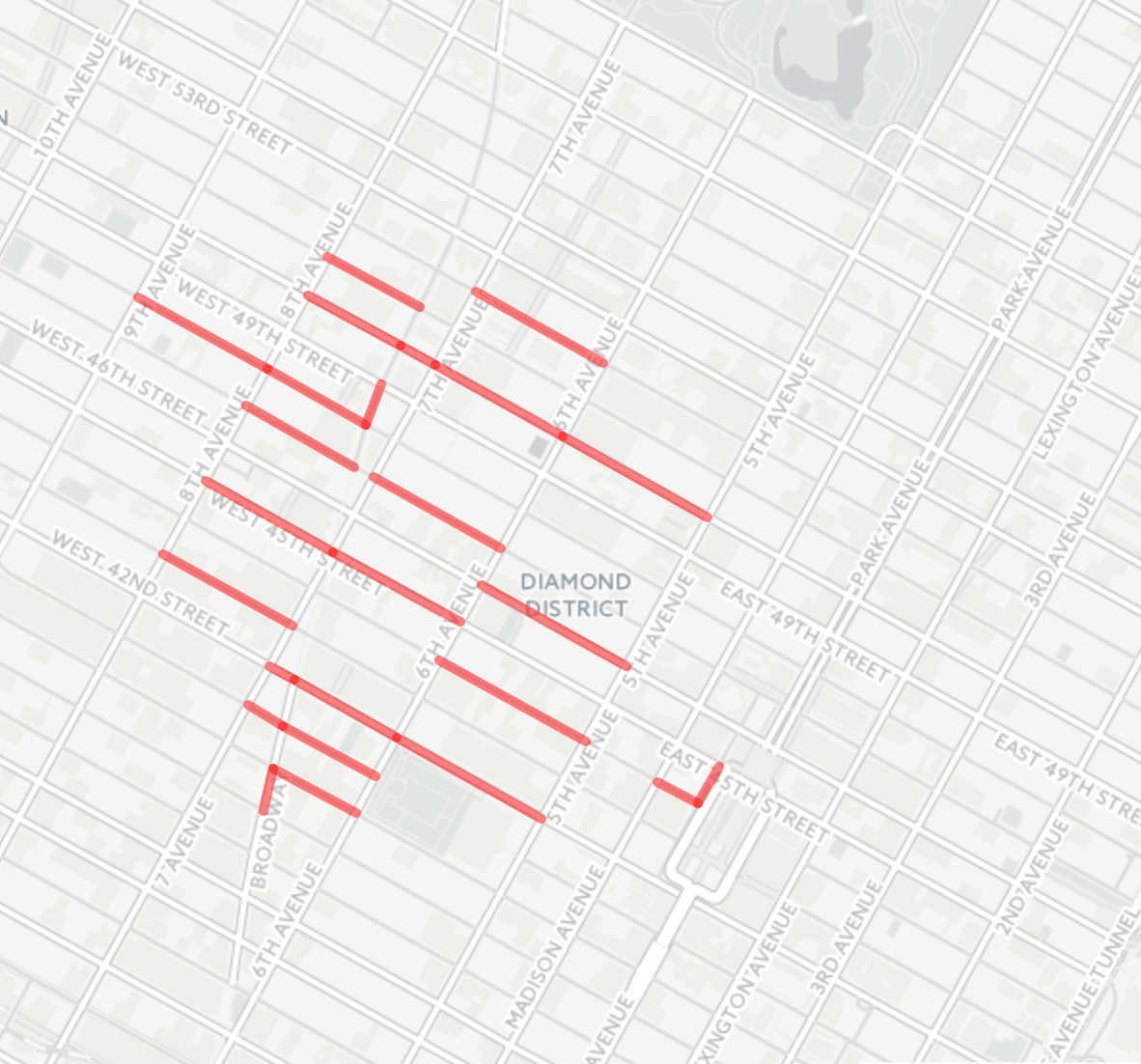
(d) Roads with speeds in $[2.5,3)$.

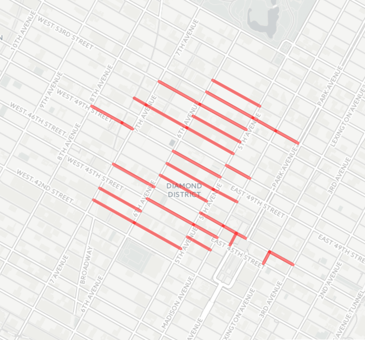
(e) Roads with speeds in $[2,2.5)$

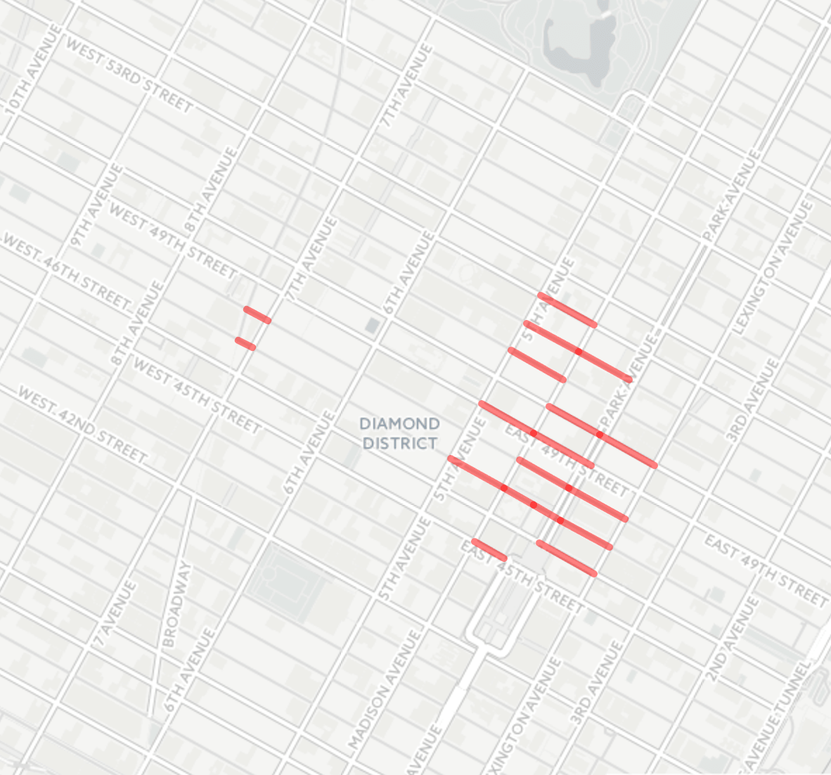
(f) Roads with speeds in $(0,2)$

Figure 3. Spatial distribution of the average road speed in the Diamond District from 9-10 AM in the summer of 2011.

Let’s look at the connectedness of the roads in Figures 3(a)–3(f). Since connectedness of the partially uncongested roads is our primary interest, the actual length of the various links plays no role. Figure 3(a) has 9 connected components, Figure 3(b) has 14 connected components, Figure 3(c) has 11 connected components and Figure 3(d) has 14 connected components. The connectivity of the components gives an idea of how ”big” a region of good or bad traffic is. Informally, traffic congestion refers to a large connected cluster of slow roads. Most of the NE-SW roads are fast (Figures 3(a)–3(c)), and the NW-SE roads are slower (Figures 3(d)–3(f)). The system seems to become a solid connected component at around 2.5.

We can reinterpret Figures 3(a)–3(f) via barcodes. Figure 4(a) consists of the roads with speeds faster than 4. We can add together the links of Figures 3(a) and 3(b) and get the roads with speeds larger than 3.5; see Figure 4(b). At the other extreme, if we augment Figure 3(d) with all the roads with speeds at least 2.5, we get Figure 4(d). Figure 1 implicitly consists of all roads with nonnegative speeds.

(a) Roads with speeds in $[4,\infty)$. There are 9 connected components.

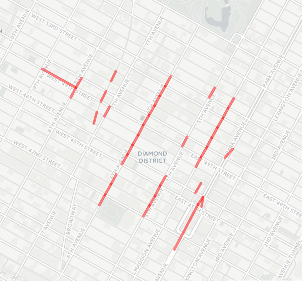
(b) Roads with speeds in $[3.5,\infty)$. There are 14 connected components.

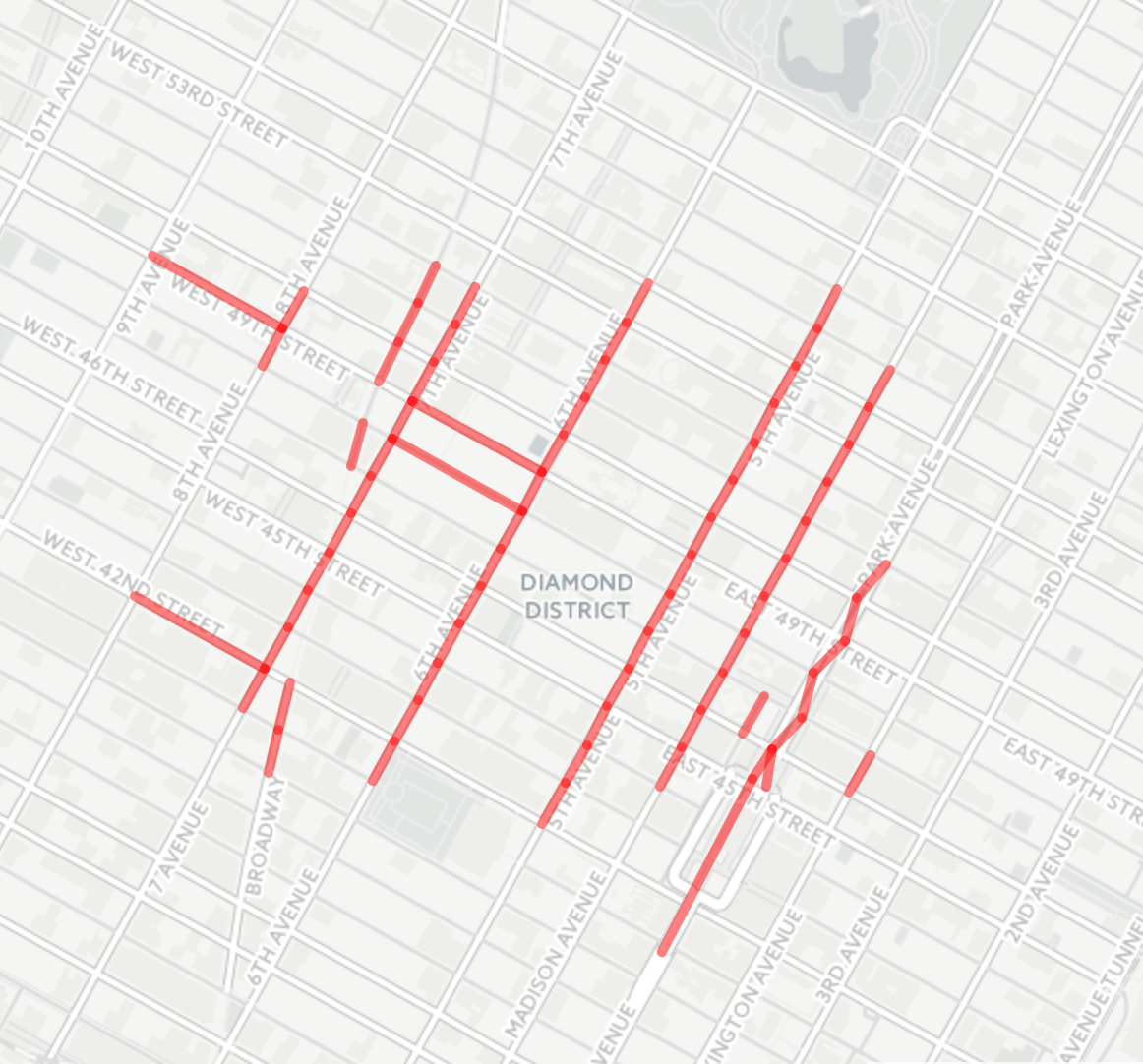
(c) Roads with speeds in $[3,\infty)$. There are 10 connected components.

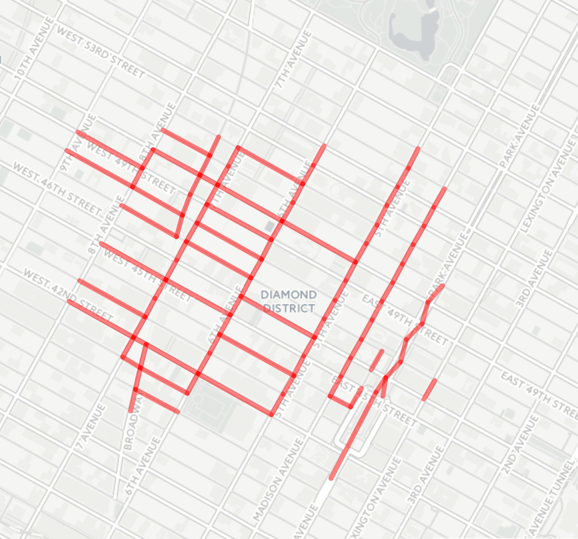
(d) Roads with speeds in $[2.5,\infty)$. There are 5 connected components.

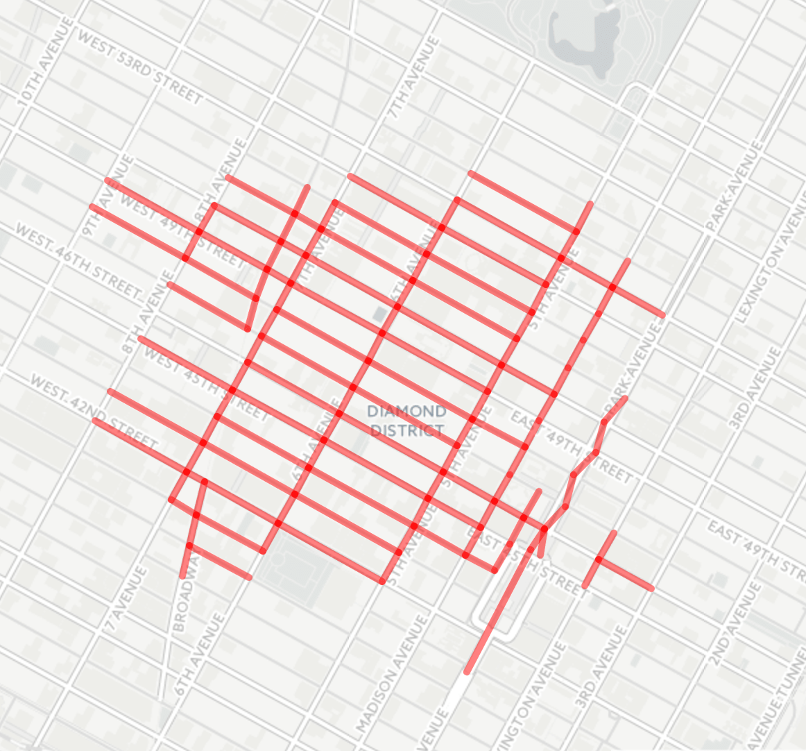
(e) Roads with speeds in $[2,\infty)$. There are 2 connected components.

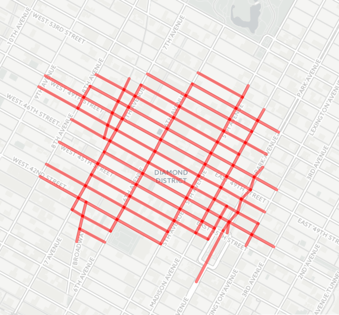
(f) Roads with speeds in $(0,\infty)$. There is one connected component.

Figure 4. $G(\lambda)$ for $\lambda\in\{4,3.5,3,2.5,2,0\}$

The barcode for the Diamond district is in Figure 5. Reflecting Figures 4(a)–4(f), there are nine bars above $\lambda=4$, 14 bars above $\lambda=3.5$ (some start or end close to 3.5), 10 bars above $\lambda=3$ (some end near 3), five bars above 2.5, two bars above 2, and one bar above 0. There is a fair amount of instability near 3.5. Connected components appear, before being merged into other connected components. There are about 7 ’long’ bars (longer than length about 1). We can think of these as robust components. Three connected regions with speeds larger than about 2, but beyond, all of the diamond district becomes one connected component.

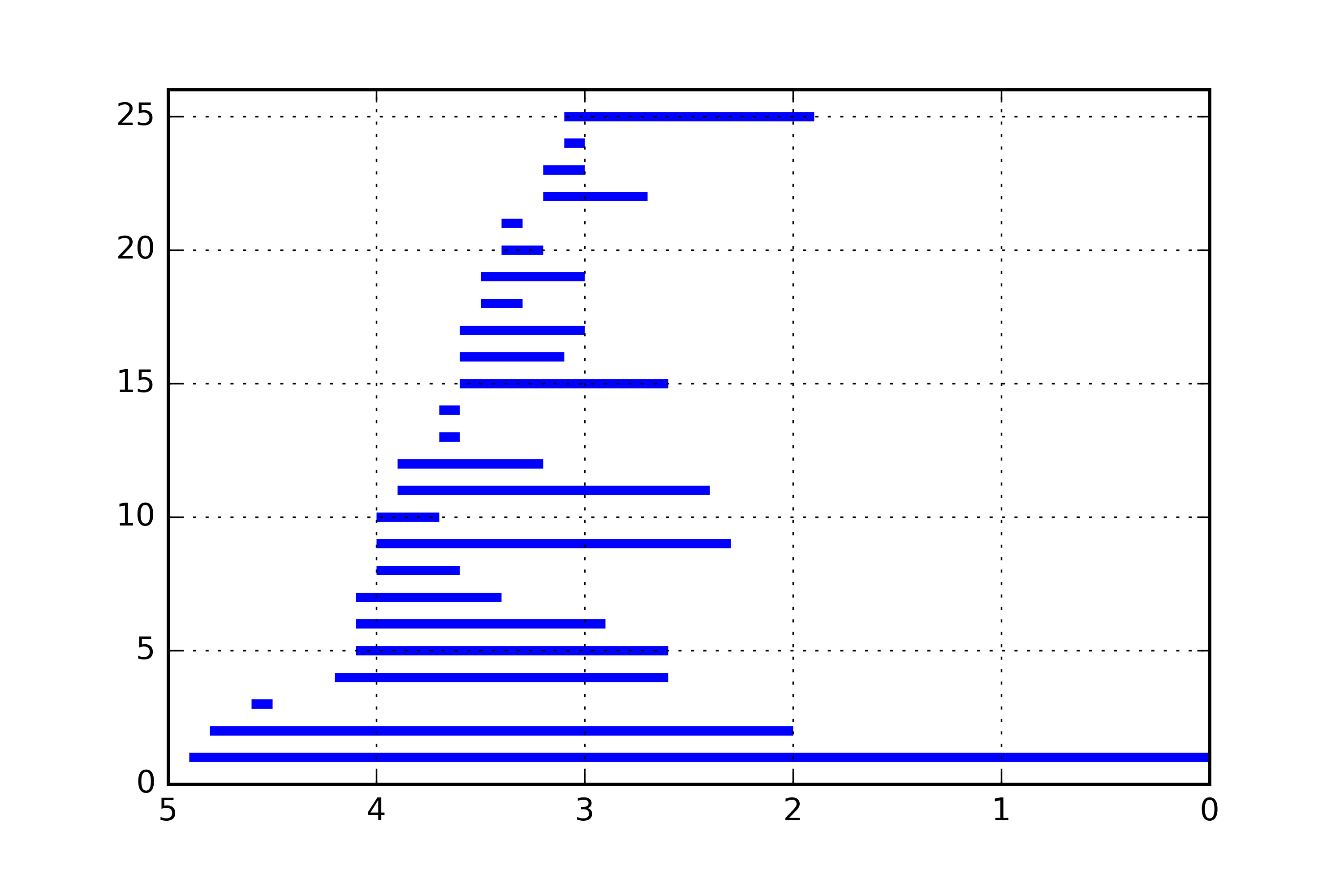
Figure 5. barcode diagram for Diamond District. Horizontal axis is $\lambda$, and vertical axis is the list index in barcode.

5. Conclusions and future work

We have developed a barcode representation of congestion of a reduced dataset. This visualization gives an alternate way of looking at connectedness of congestion and gives us an understanding of robustness of congestion.

Applying this technique to Diamond District in New York shows that there are only a few small pockets where speeds are above 4 m/s, whereas in most of the region the speeds are between 2 and 4 m/s (Table 1). It also shows that speeds are faster on North-South “Avenues” than on East-West “Streets”. These observations can be compared with neighboring areas and can show whether Diamond District is more or less congested than surrounding areas during observed times and if it offers greater uniformity in travel speeds.

This technique can also be applied to a much larger network of roads and in combination with other factors such as, time of day. For example, if a trip originates north of the Diamond District and concludes south of it during the evening rush hour, and the traveler has the option to either drive through or around the district, an understanding of congestion and variability of speeds during that time would assist in deciding an appropriate route. Overall, such analysis could also help identify areas in a city where traffic is significantly faster and areas that are severely congested, in turn assisting drivers avoid some areas, if possible, or plan for extra time. For planners, understanding the pattern, severity, and frequency of such congestion may help identify locations where infrastructure upgrade or congestion relief measures may be needed. For first responders, areas of chronic congestion may require additional resources or contingency plans.

Table 1. Observations under different speed thresholds

Although our dataset is small enough that direct visual inspection of speeds on maps is feasible, our techniques can give quantifiable information for larger and more complex datasets.

The notion of persistence can be taken in several new directions. In this dataset, we have ignored directionality of streets (which in our case affects only a small number of streets). A proper treatment of direction requires deeper theoretical innovations and will be developed elsewhere.

An interesting aspect of persistent homology lies in understanding the effects of boundaries. The roads in a network surround land which has a variety of uses. One might, for example, fill in land which has a certain population density. That would leadto thinking of roads as networks which allow inhabitants access to neighborhoods. One might also turn around and think of congestion as obstacles, much as in the robotics path planning work of [9].

References

- [1] J. A. Deri and J. M. F. Moura. Taxi data in new york city: A network perspective. In 2015 49th Asilomar Conference on Signals, Systems and Computers, pages 1829–1833, Nov 2015.
- [2] Yuan Zhu, Kaan Ozbay, Kun Xie, and Hong Yang. Using big data to study resilience of taxi and subway trips for hurricanes sandy and irene. Transportation Research Record: Journal of the Transportation Research Board, (2599):70–80, 2016.
- [3] Xianyuan Zhan, Satish V. Ukkusuri, and Feng Zhu. Inferring urban land use using large-scale social media check-in data. Networks and Spatial Economics, 14(3):647–667, 2014.
- [4] Xiangyang Guan, Cynthia Chen, and Dan Work. Tracking the evolution of infrastructure systems and mass responses using publicly available data. PloS one, 11(12):e0167267, 2016.
- [5] Javier Alonso-Mora, Samitha Samaranayake, Alex Wallar, Emilio Frazzoli, and Daniela Rus. On-demand high-capacity ride-sharing via dynamic trip-vehicle assignment. Proceedings of the National Academy of Sciences, page 201611675, 2017.
- [6] Nivan Ferreira, Jorge Poco, Huy T Vo, Juliana Freire, and Cláudio T Silva. Visual exploration of big spatio-temporal urban data: A study of new york city taxi trips. IEEE Transactions on Visualization and Computer Graphics, 19(12):2149–2158, 2013.
- [7] Chicago Data Portal taxi trips. https://data.cityofchicago.org/Transportation/Taxi-Trips/wrvz-psew.
- [8] NYC Taxi and Limousine Commission tlc trip record data.
- [9] Subhrajit Bhattacharya, Robert Ghrist, and Vijay Kumar. Persistent homology for path planning in uncertain environments. IEEE Transactions on Robotics, 31(3):578–590, 2015.
- [10] Hyekyoung Lee, Hyejin Kang, Moo K Chung, Bung-Nyun Kim, and Dong Soo Lee. Persistent brain network homology from the perspective of dendrogram. IEEE transactions on medical imaging, 31(12):2267–2277, 2012.
- [11] Mahmuda Ahmed, Brittany Terese Fasy, and Carola Wenk. Local persistent homology based distance between maps. In Proceedings of the 22nd ACM SIGSPATIAL International Conference on Advances in Geographic Information Systems, pages 43–52. ACM, 2014.
- [12] Herbert Edelsbrunner, David Letscher, and Afra Zomorodian. Topological persistence and simplification. In Foundations of Computer Science, 2000. Proceedings. 41st Annual Symposium on, pages 454–463. IEEE, 2000.
- [13] Afra Zomorodian and Gunnar Carlsson. Computing persistent homology. Discrete Comput. Geom., 33(2):249–274, 2005.
- [14] Dane Taylor, Florian Klimm, Heather A. Harrington, Miroslav Kramár, Konstantin Mischaikow, Mason A. Porter, and Peter J. Mucha. Topological data analysis of contagion maps for examining spreading processes on networks. Nature Communications, 6:7723 EP –, Jul 2015. Article.
- [15] Herbert Edelsbrunner and John Harer. Persistent homology-a survey. Contemporary mathematics, 453:257–282, 2008.
- [16] Robert Ghrist. Barcodes: the persistent topology of data. Bulletin of the American Mathematical Society, 45(1):61–75, 2008.
- [17] Gunnar Carlsson, Tigran Ishkhanov, Vin De Silva, and Afra Zomorodian. On the local behavior of spaces of natural images. International journal of computer vision, 76(1):1–12, 2008.
- [18] Pawel Dłotko, Robert Ghrist, Mateusz Juda, and Marian Mrozek. Distributed computation of coverage in sensor networks by homological methods. Applicable Algebra in Engineering, Communication and Computing, 23(1-2):29–58, 2012.
- [19] Andrew Banman and Lori Ziegelmeier. Mind the gap: A study in global development through persistent homology. arXiv preprint arXiv:1702.08593, 2017.
- [20] Robert Ghrist. Barcodes: the persistent topology of data. Bull. Amer. Math. Soc. (N.S.), 45(1):61–75, 2008.
- [21] James R Munkres. Elements of algebraic topology, volume 2. Addison-Wesley Menlo Park, 1984.
- [22] Shimon Even. Graph algorithms. Cambridge University Press, 2011.
- [23] Brian Donovan and Daniel B Work. Using coarse gps data to quantify city-scale transportation system resilience to extreme events. arXiv preprint arXiv:1507.06011, 2015.