A Two-Stage Architecture for Differentially Private Kalman Filtering and LQG Control

Abstract

Large-scale monitoring and control systems enabling a more intelligent infrastructure increasingly rely on sensitive data obtained from private agents, e.g., location traces collected from the users of an intelligent transportation system. In order to encourage the participation of these agents, it becomes then critical to design algorithms that process information in a privacy-preserving way. This article revisits the Kalman filtering and Linear Quadratic Gaussian (LQG) control problems, subject to privacy constraints. We aim to enforce differential privacy, a formal, state-of-the-art definition of privacy ensuring that the output of an algorithm is not too sensitive to the data collected from any single participating agent. A two-stage architecture is proposed that first aggregates and combines the individual agent signals before adding privacy-preserving noise and post-filtering the result to be published. We show a significant performance improvement offered by this architecture over input perturbation schemes as the number of input signals increases and that an optimal static aggregation stage can be computed by solving a semidefinite program. The two-stage architecture, which we develop first for Kalman filtering, is then adapted to the LQG control problem by leveraging the separation principle. Numerical simulations illustrate the performance improvements over differentially private algorithms without first-stage signal aggregation.

I Introduction

To monitor and control intelligent infrastructure systems such as smart grids, smart buildings or smart cities, data needs to be continuously collected from the people interacting with these systems, either through sensors installed in the environment such as cameras and smart meters, or through personal devices such as smartphones. Hence, in contrast to more traditional control systems, the measured signals for such systems often contain highly privacy-sensitive information, e.g., related to the real-time location or health of a person. For example, the accuracy of crowd-sourced traffic maps and congestion-aware routing applications is increased by using data provided by smartphones and connected vehicles [2]. However, individual location data turns out to be very difficult to properly anonymize because individuals have highly unique mobility patterns [3, 4], and in fact individual trajectories can be reconstructed even from just aggregate location data [5, 6]. Similarly, fine-grained measurements of a house’s electric power consumption collected by a smart meter can enable demand-response schemes, but can also be used to infer the activities of the occupants, by identifying the usage of individual appliances [7, 8, 9, 10]. Therefore, it is necessary to implement privacy-preserving mechanisms when sensitive data must be shared to improve a system’s performance.

Various definitions of privacy have been proposed that are amenable to formal analysis. While a survey of such definitions is out of the scope of this paper, we can mention some recent work focusing on signal processing and control problems. Privacy is measured by a lower bound on the mutual information between published and private signals in [11], on the Fisher information in [12], or on the error covariance of the estimator of a sensitive signal in [13, 14]. The concept of $k$-anonymity and its extensions has been applied to the publication of location traces in [15]. But much of the recent research on privacy-preserving data analysis relies on the notion of differential privacy [16, 17, 18]. In the standard set-up, which is also the situation considered in this article, a data holder aims to release the results of computations based on private data. Differential privacy is enforced by adding an appropriate amount of noise to the published results, in such a way that the probability distribution over the outputs does not depend too much on the data of any single individual. As a result, the ability of a third party observing the outputs to make new inferences about a given person is roughly the same, whether or not that person chooses to contribute its data. This guarantee can then be used to weigh the risks of information disclosure against the benefits of publishing more accurate analyses.

A large number of techniques have been developed to compute differentially private versions of various statistics, see [18] for an overview. Nevertheless, the differentially private analysis of streaming data remains relatively less explored [19, 11, 20], despite its importance for signal processing and control applications. Some previous work has focused on the design of differentially private dynamic estimators [21, 22, 23, 24], controllers [25, 26], consensus algorithms [27, 28], or anomaly detectors [29, 30, 31]. In particular, [21] discusses the Kalman filtering problem under a differential privacy constraint and compares schemes introducing noise either directly on the measured signals (input perturbation mechanisms) or on the published estimate (output perturbation mechanisms). Output perturbation provides better performance as the number of input signals increases, but has the drawback of leaving unfiltered noise on the output, which motivates the two-stage architecture that we consider here. In [25], the authors consider a multi-agent linear quadratic tracking problem where the trajectory tracked by each agent should remain private, while [26] considers an LQG control problem where each agent wishes to keep its individual state private. In both cases, noise is added directly on the individual measurements, a form of input perturbation.

In this paper we study the design of Kalman filters and LQG controllers subject to a differential privacy constraint on the measured signals. These problems, stated formally in Section II, arise when a data collector measures private signals originating from a population of agents, whose dynamics can be modeled as linear Gaussian systems, in order to publish in real-time either an estimate of an aggregate state of the agent population, or a control signal shared by the agents and aimed at regulating such an aggregate state. As a motivating example, one can consider the problem of controlling the distribution of vehicles on a road network by means of traffic messages broadcasted to all cars, with the current density estimated from location data obtained from the smartphones of individual drivers.

Section III presents the main contribution of this paper, namely, a two-stage architecture for differentially private Kalman filtering, where the privacy-preserving noise is added only after an input stage appropriately combining the measured signals of the individual agents, while an output stage filters out this noise. Such two-stage architectures were discussed in [21] but have not yet been applied to the Kalman filtering problem, and we argue first in Section III-A via a simple example that significant performance improvements can be expected compared to input perturbation mechanisms. We show that the optimal input stage can be computed by solving a semidefinite program (SDP), hence, a tractable convex optimization problem. The fact that the input stage design problem admits an SDP formulation is reminiscent of other Kalman filtering problems subject to resource or communication constraints, see, e.g., [32, 33, 34], but the SDP capturing specifically the differential privacy constraint is new. The design procedure is then adapted in Section IV to the LQG control problem. By exploiting the classical properties of the optimal LQG controller (linearity and separation principle), we can view the control problem as the problem of estimating a certain linear combination of the agent states as in Section III, but for a specific cost on the estimation error.

A conference version of this paper appeared in [1], but contained no proof and did not discuss the LQG control problem. The numerical examples discussed in Sections III-D and IV-B are also new. Finally, we introduce some notation used throughout this paper. We fix a generic probability triple $(\Omega,\mathcal{F},\mathbb{P})$, where $\mathcal{F}$ is a $\sigma$-algebra on $\Omega$ and $\mathbb{P}$ a probability measure defined on $\mathcal{F}$. The notation $X\sim\mathcal{N}(\mu,\Sigma)$ means that $X$ is a Gaussian random vector with mean vector $\mu$ and covariance matrix $\Sigma$. “Independent and identically distributed” is abbreviated iid. We denote the $p$-norm of a vector $x\in\mathbb{R}{}^{k}$ by $|x|_{p}:=(\sum_{i=1}^{k}|x_{i}|^{p})^{1/p}$, for $p\in[1,\infty)$. For a matrix $A$, the induced 2-norm (maximum singular value of $A$) is denoted $\|A\|_{2}$ and the Frobenius norm $\|A\|_{F}:=\sqrt{\text{Tr}(A^{\text{T}}A)}$. If $A$ and $B$ are symmetric matrices, $A\succeq B$ (resp. $A\succ B$) means that $A-B$ is positive semi-definite (resp. positive definite). We use the notation $\text{diag}(A_{1},\ldots,A_{n})$ to represent a block-diagonal matrix with the matrices $A_{i}$ on the diagonal. The column vector of size $n$ with all components equal to $1$ is denoted $\mathbf{1}_{n}$. Finally, for a discrete-time signal $x$ we denote $x_{0:t}:=\{x_{0},\ldots,x_{t}\}$.

II Problem Statement

II-A Privacy-Preserving State Estimation and LQG Control for a Population of Dynamic Agents

Consider a set of $n$ privacy-sensitive signals $\{y_{i,t}\}_{0\leq t\leq T}$, $i=1,\ldots,n$, with $y_{i,t}\in\mathbb{R}^{p_{i}}$, collected by a data aggregator, and which could originate from $n$ distinct agents. Let $p=\sum_{i=1}^{n}p_{i}$. We assume that a mathematical model capturing known dynamic and statistical properties of these signals is publicly available, consisting of a linear system with $n$ independent (vector-valued) states associated to the $n$ measured signals

$$\begin{split}x_{i,t+1}&=A_{i,t}\,x_{i,t}+B_{i,t}\,u_{t}+w_{i,t},\;\;0\leq t\leq T-1,\\ y_{i,t}&=C_{i,t}\,x_{i,t}+v_{i,t},\;\;0\leq t\leq T,\end{split}$$ (1)

for $i=1,\ldots,n$, where $x_{i,t},w_{i,t}\in\mathbb{R}^{m_{i}}$. Here $w_{i,t}\sim\mathcal{N}(0,W_{i,t})$ and $v_{i,t}\sim\mathcal{N}(0,V_{i})$ are independent sequences of iid zero-mean Gaussian random vectors with covariance matrices $W_{i,t}\succ 0,V_{i}\succ 0$, for $i=1,\ldots,n$. In particular, assuming that the matrices $W_{i,t}$ are invertible is necessary in the following to be able to use the “information filter” form of the Kalman filter equations [35]. The sequence $u$ with $u_{t}\in\mathbb{R}^{h}$ represents a control input that is shared by the $n$ individuals. This is motivated by scenarios in which a common signal is broadcast to drive the aggregate state of a population, while individual signals can still be subject to privacy constraints. The initial conditions $x_{i,0}$ are independent Gaussian random vectors that are also independent of the noise processes $w$ and $v$, with mean $\overline{x}_{i,0}$ and covariance matrices $\Sigma_{i,0}^{-}\succ 0$. Let $x_{t}:=[x_{1,t}^{T},\ldots,x_{n,t}^{T}]^{T}$, $y_{t}:=[y_{1,t}^{T},\ldots,y_{n,t}^{T}]^{T}$, $w_{t}=[w_{1,t}^{T},\ldots,w_{n,t}^{T}]^{T}$ and $v_{t}=[v_{1,t}^{T},\ldots,v_{n,t}^{T}]^{T}$ denote the global state, measurement and noise signals of (1). Define $A_{t}:=\textup{diag}(A_{1,t},\ldots,A_{n,t})$, $B_{t}=[B_{1,t}^{T},\ldots,B_{n,t}^{T}]^{T}$, $C_{t}=\textup{diag}(C_{1,t},\ldots,C_{n,t})$, $W_{t}=\textup{diag}(W_{1,t},\ldots,W_{n,t})$, $V=\textup{diag}(V_{1},\ldots,V_{n})$. Then the system (1) can be rewritten more compactly as

$$x_{t+1} =A_{t}\,x_{t}+B_{t}\,u_{t}+w_{t},\;\;0\leq t\leq T-1,$$ (2)

$$y_{t} =C_{t}\,x_{t}+v_{t},\;\;0\leq t\leq T,$$ (3)

with $w_{t}\sim\mathcal{N}(0,W_{t})$ and $v_{t}\sim\mathcal{N}(0,V)$. Throughout the paper, the model parameters $\overline{x}_{i,0}$, $\Sigma^{-}_{i,0}$, $A_{i,t}$, $B_{i,t}$, $C_{i,t}$, $W_{i,t}$, $V_{i}$, are assumed to be publicly known information.

In Section III, we first consider a filtering problem (with $u$ a known signal) where the data aggregator aims to publish at each period $t$ a causal estimate $\hat{z}_{t}$ of a linear combination $z_{t}=L_{t}x_{t}=\sum_{i=1}^{n}L_{i,t}x_{i,t}$ of the individual states, computed from the signals $y_{i}$, with $L_{t}:=\begin{bmatrix}L_{i,t},\ldots,L_{n,t}\end{bmatrix}$ some given (publicly known) matrices. This estimator should minimize the Mean Square Error (MSE) performance measure

$$E_{T}:=\frac{1}{T+1}\sum_{t=0}^{T}\mathbb{E}\left[\|z_{t}-\hat{z}_{t}\|_{2}^{2}\right].$$ (4)

For privacy reasons, the signals $y_{i}$ are not released by the data aggregator and moreover the publicly released estimate $\hat{z}$ should also guarantee the differential privacy of the input signals $y_{i}$, as defined precisely in Section II-B. For example, the signals $y_{i}$ could represent position measurements of $n$ individuals, each state $x_{i}$ could consist of the position and velocity of individual $i$, and the goal might be to publish only a real-time estimate of the average velocity of all individuals. Note that in the absence of privacy constraint, the optimal estimator is $\hat{z}_{t}=\sum_{i=1}^{n}L_{i,t}\hat{x}_{i,t}$, with $\hat{x}_{i,t}$ provided by the (time-varying) Kalman filter estimating the state $x_{i}$ of subsystem $i$ from the signal $y_{i}$ [35], and in particular the estimation problem then decouples for the $n$ subsystems.

Next, in Section IV we build on the results obtained for the filtering problem to study the following privacy-constrained Linear Quadratic Gaussian (LQG) regulation problem. The data aggregator uses the measured signals $y_{i},1\leq i\leq n$, to compute and broadcast a (causal) control signal $u$ that minimizes the following quadratic cost for the $n$ agents

$$J_{T}=\frac{1}{T+1}\mathbb{\mathbb{E}}\left[\sum_{t=0}^{T-1}\left(x_{t}^{T}Q_{t}x_{t}+u_{t}^{T}R_{t}u_{t}\right)+x_{T}^{T}Q_{T}x_{T}\right],$$ (5)

where $Q_{t}\succeq 0$ for $0\leq t\leq T$ and $R_{t}\succ 0$ for $0\leq t\leq T-1$ are publicly known weight matrices. Again, only the signal $u$ is published (in particular, it is available to the $n$ agents), and releasing $u$ must guarantee the differential privacy of the measured signals $y_{i}$. It is worth noting that the cost function (5) can be used to drive an aggregate value of the global population state toward $0$ rather than the individual agent states, since trying to do the latter might be in direct conflict with the privacy requirement (which, essentially, aims to hide the value of the individual signals $y_{i}$, and hence indirectly of the individual states $x_{i}$). For example, we can have $x_{t}Q_{t}x_{t}=\left(\frac{1}{n}\sum_{i=1}^{n}x_{i,t}\right)^{2}$ if $Q_{t}=\frac{1}{n^{2}}\mathbf{1}_{n}\mathbf{1}_{n}^{T}$, in order to regulate the average population state. Figure 1 represents the estimation and control problem setups, including a basic scheme to enforce differential privacy by injecting noise directly in the signals $\{y_{i}\}_{1\leq i\leq n}$, as described in Section II-C.

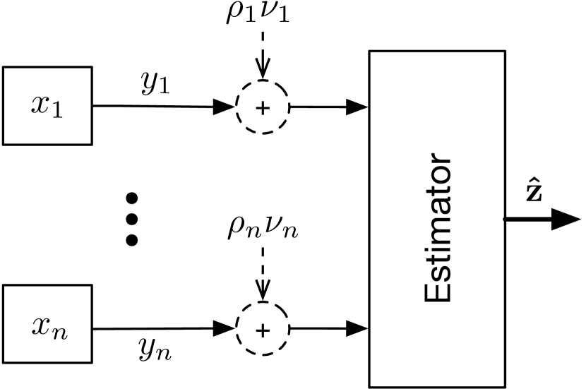
(a) Estimation Problem

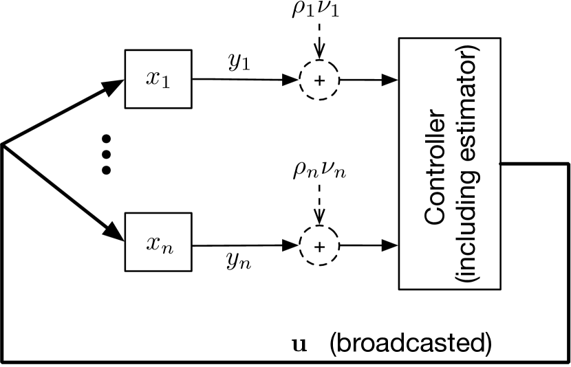
(b) Control Problem

Figure 1: Estimation and control problem setup. Signals $\{y_{i}\}_{1\leq i\leq n}$ produced by $n$ independent agents with states $\{x_{i}\}_{1\leq i\leq n}$ are collected for monitoring or control purposes. The thicker lines correspond to published signals (estimate $\hat{z}$ or broadcasted control input $u$). Dashed lines represent the injection of privacy-preserving noise by the input perturbation mechanism, a simple scheme to enforce differential privacy described in Section II-C.

Note that the steady-state versions of both the filtering and LQG control problems are also considered, with the model (2)-(3) in this case assumed time-invariant and the performance measures defined as

$$E_{\infty}:=\lim_{T\to\infty}E_{T},\;\;J_{\infty}:=\lim_{T\to\infty}J_{T}.$$ (6)

To finish stating the above problems formally, we define in the next section the differential privacy constraint imposed on the signal $\hat{z}$ for the filtering problem and $u$ for the LQG problem.

II-B Differential Privacy Constraint

Differential privacy [18] is a property satisfied by certain randomized algorithms (also called mechanisms), which in an abstract setting compute outputs in a space $\mathsf{R}$ based on sensitive data in a space $\mathsf{D}$. To be differentially private, the algorithm must ensure that the probability distribution of its randomized output is not very sensitive to certain variations in the input data, which are specified as part of the privacy requirement.

More concretely, we equip the input space $\mathsf{D}$ with a symmetric binary relation called adjacency and denoted Adj, which captures the variations in the input datasets that we want to make hard to detect by observing the outputs. In our case, the input space $\mathsf{D}$ is the vector space $\mathbb{R}^{p(T+1)}$ of global measurement signals $y$, and a mechanism is a causal stochastic system producing an output signal ($\hat{z}$ or $u$ in the previous section) based on its input $y$. We define two measured signals to be adjacent if the following condition holds

$$\begin{split}\text{Adj}(y,y^{\prime})\,\text{iff for some}\,1\leq i\leq n,\,\|y_{i}-y_{i}^{\prime}\|_{2}\leq\rho_{i},\\ \text{and}\,y_{j}=y_{j}^{\prime}\,\text{for all}\,j\neq i,\end{split}$$ (7)

with $\{\rho_{i}\}_{i=1}^{n}\in\mathbb{R}_{+}^{n}$ a given set of positive numbers and with the definition of the $\ell_{2}$-norm $\|v\|_{2}:=\left(\sum_{t=0}^{T}|v_{t}|_{2}^{2}\right)^{1/2}$ for a vector-valued signal $v$. In other words, two adjacent measurement signals can differ by the values of a single participant, with only $\ell_{2}$-bounded signal deviations allowed for each individual. For any two inputs that satisfy the adjacency relation, the following definition characterizes the deviation that is allowed for a differentially private mechanism’s output distribution.

Definition 1.

Let $\mathsf{D}$ be a space equipped with a symmetric binary relation denoted Adj and let $(\mathsf{R},\mathcal{R})$ be a measurable space, where $\mathcal{R}$ is a given $\sigma$-algebra over $\mathsf{R}$. Let $\epsilon\geq 0$, $1\geq\delta\geq 0$. A randomized mechanism $M$ from $\mathsf{D}$ to $\mathsf{R}$ is $(\epsilon,\delta)$-differentially private (for Adj) if for all $d,d^{\prime}\in\mathsf{D}$ such that $\text{Adj}(d,d^{\prime})$,

$$\mathbb{P}(M(d)\in S)\leq e^{\epsilon}\,\mathbb{P}(M(d^{\prime})\in S)+\delta,\,\forall S\in\mathcal{R}.$$ (8)

In Definition 1, smaller values of $\epsilon$ and $\delta$ correspond to stronger privacy guarantees, i.e., distributions for $M(d)$ and $M(d^{\prime})$ that are closer in (8). Next, we need tools that can be used to enforce the property of Definition 1. The following definition is useful for mechanisms such as ours that produce outputs in vector spaces.

Definition 2.

Let $\mathsf{D}$ be a space equipped with an adjacency relation Adj. Let $\mathsf{R}$ be a vector space equipped with a norm $\|\cdot\|_{\mathsf{R}}$. The sensitivity of a mapping $q:\mathsf{D}\mapsto\mathsf{R}$ is defined as

$$\triangle q:=\sup_{\{d,d^{\prime}:\text{Adj}(d,d^{\prime})\}}\|q(d)-q(d^{\prime})\|_{\mathsf{R}}.$$

For $\mathsf{R}=\mathbb{R}^{h(T+1)}$ or $(\mathbb{R}^{h})^{\mathbb{N}}$ equipped with the $\ell_{2}$-norm, this defines the $\ell_{2}$-sensitivity of $q$, denoted $\triangle_{2}q$.

The Gaussian mechanism [36] consists in adding Gaussian noise proportional to the $\ell_{2}$-sensitivity of a mapping to enforce $(\epsilon,\delta)$-differential privacy. A fairly tight upper bound on the proportionality constant is provided in [21]. Recall first the definition of the $\mathcal{Q}$-function $\mathcal{Q}(x):=\frac{1}{\sqrt{2\pi}}\int_{x}^{\infty}\exp(-\frac{u^{2}}{2})du$, which is monotonically decreasing from $(-\infty,\infty)$ to $(0,1)$. Then, for $1>\delta>0$, define $\kappa_{\delta,\epsilon}:=\frac{1}{2\epsilon}\left(Q^{-1}(\delta)+\sqrt{(Q^{-1}(\delta))^{2}+2\epsilon}\right)$. The following theorem can be found in [21].

Theorem 1.

Let $\epsilon>0$, $1>\delta>0$. Let $G$ be a dynamic system with $p$ inputs and $q$ outputs. Then the mechanism $M(y)=Gy+\nu$, where $\nu$ is a white Gaussian noise (sequence of iid zero-mean Gaussian vectors) with $\nu_{t}\sim\mathcal{N}(0,\kappa_{\delta,\epsilon}^{2}(\Delta_{2}G)^{2}I_{q})$, is $(\epsilon,\delta)$-differentially private.

In other words, Theorem 1 says that we can produce a differentially private signal by adding white Gaussian noise at the output of a system $G$ processing the sensitive signal $y$, with covariance matrix $\sigma^{2}I_{q}$, and $\sigma$ proportional to the $\ell_{2}$-sensitivity of $G$.

II-C A First Solution: Input Perturbation Mechanism

An important property of differential privacy is its resilience to post-processing [18], i.e., applying further computations to an output that is differentially private does not degrade the differential privacy guarantee, as long as the original dataset is not reaccessed for these computations. This leads immediately to a first solution for the estimation and control problems stated in the previous section, called the input perturbation mechanism, which consists in perturbing each measured signal $y_{i}$ directly to release differentially private versions of these signals.

First, note that the memoryless system defined by $(Gy)_{t}=My_{t}$, where $M$ is the diagonal matrix $M=\text{diag}(1/\rho_{1},\ldots,1/\rho_{n})$, has the sensibility bound

$$\Delta G:=\sup_{\text{Adj(y,y')}}\|My-My^{\prime}\|_{2}\leq 1$$

for the adjacency relation (7). Hence, by Theorem 1, releasing the signals $\{y_{i}/\rho_{i}+\nu_{i}\}_{1\leq i\leq n}$, where each signal $\nu_{i}$ is a white Gaussian noise with covariance matrix $\kappa_{\delta,\epsilon}^{2}I_{p_{i}}$, is $(\epsilon,\delta)$-differentially private. Equivalently, using the resilience to post-processing to multiply this output by $M^{-1}$, we see that releasing the signals $\{\tilde{y}_{i}:=y_{i}+\rho_{i}\nu_{i}\}_{1\leq i\leq n}$ is $(\epsilon,\delta)$-differentially private. Once these signals are released, applying further processing on them does not impact the differential privacy guarantee. Moreover, these signals are of the same form as the outputs of system (1), except for a higher level of (still Gaussian) noise due to the addition of the artificial privacy-preserving noise. One can therefore produce an $(\epsilon,\delta)$-differentially private estimate $\hat{z}$ or control signal $u$ discussed in Section II-A by applying standard Kalman filtering and LQG design techniques to the signals $\tilde{y}_{i}$, see Figure 1. An advantage of input perturbation mechanisms is that each agent can release directly the differentially private signal $\tilde{y}_{i}$, and hence does not need to trust the data aggregator to enforce the differential privacy property. Moreover, this mechanism has the potentially useful feature of publishing the individual signals $\tilde{y}_{i}$, which could be used for other purposes than the original estimation or control problem. Nonetheless, as we discuss in the following sections, input perturbation typically leads to a high level of noise and hence performance degradation, which motivates the search for better mechanisms.

III Differentially Private Kalman Filtering

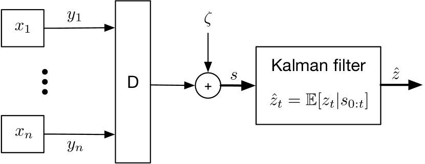
Figure 2: Differentially private Kalman filtering architecture with first-stage aggregation. $D$ is a matrix to design, used to combine the individual measured signals appropriately. The signal $s$ is differentially private ($\zeta$ is a privacy-preserving white Gaussian noise signal), and so is the released estimate $\hat{z}$ by resilience to post-processing.

Input perturbation for the differentially private Kalman filtering problem, as discussed in Section II-C and represented on Figure 1(a), was considered in [37]. Here, we show first in Section III-A via a simple example that the performance of this mechanism can be significantly improved by combining the individual input signals before adding the privacy preserving noise. This leads to the two-stage mechanism of Figure 2, whose systematic design is discussed in Section III-B.

III-A A Scalar Example

Consider a scalar homogeneous version of model (1) with $A_{i,t}=a\in\mathbb{R}$, $B_{i,t}=b$, $C_{i,t}=c$, $W_{i,t}=\sigma_{w}^{2}$, $V_{i}=\sigma_{v}^{2}$ and $L_{i,t}=1$ (so $z_{t}=\sum_{i=1}^{n}x_{i,t}$), and assume $\rho_{i}=\rho$ for all $i$ in (7). In other words, $A_{t}=aI_{n}$, $B_{t}=b\mathbf{1}_{n}$, $C_{t}=cI_{n}$, $W_{t}=\sigma_{w}^{2}I_{n}$, $V=\sigma_{v}^{2}I_{n}$ in (2). We also let $T\to\infty$ in the problem statement and consider the steady-state MSE $E_{\infty}$, see (6), as performance measure for a given estimator $\hat{z}$ of $z$. Moreover in this section we consider for simplicity the minimum mean square error (MMSE) estimate $\hat{z}_{t}$ of $x_{t}$ given the measurements up to time $t-1$ only, since the corresponding MSE is directly obtained by solving an algebraic Riccati equation (ARE).

Let $\alpha:=\kappa_{\delta,\epsilon}\,\rho$. Since $\sup_{y,y^{\prime}:\text{Adj}(y,y^{\prime})}\left\|y-y^{\prime}\right\|_{2}=\rho$, by Theorem 1 and as explained in Section II-C, releasing the signal $r_{t}=y_{t}+\nu_{t}$, with white noise $\nu$ such that $\nu_{t}\sim\mathcal{N}(0,\alpha^{2}I_{n})$, is $(\epsilon,\delta)$-differentially private for the adjacency relation (7). The steady-state MSE of a Kalman filter estimating $z$ for the system with dynamics as in (2) and measurements $r$ is obtained by solving a scalar ARE, which leads to the following expression

$$E_{\infty}^{1}=\frac{n}{2c^{2}}\left(-\beta+\sqrt{\beta^{2}+4(\alpha^{2}+\sigma_{v}^{2})\sigma_{w}^{2}c^{2}}\right),$$ (9)

where $\beta=(1-a^{2})(\sigma_{v}^{2}+\alpha^{2})-c^{2}\sigma_{w}^{2}$.

Instead of input perturbation, we can use the architecture shown on Fig. 2 with $D=\mathbf{1}_{n}^{T}$, a $1\times n$ row vector of ones. Consider the same adjacency relation (7) and denote $\eta_{t}=Dy_{t}=\sum_{i=1}^{n}y_{i,t}$, $\theta_{t}=\sum_{i=1}^{n}w_{i,t}$ and $\lambda_{t}=\sum_{i=1}^{n}v_{i,t}$. We have

$$z_{t+1} =az_{t}+\theta_{t},$$

$$\eta_{t} =cz_{t}+\lambda_{t}.$$

Since again $\sup_{y,y^{\prime}:\text{Adj}(y,y^{\prime})}\left\|Dy-Dy^{\prime}\right\|_{2}=\rho$, releasing the scalar signal $s_{t}=\eta_{t}+\zeta_{t}$, with $\zeta_{t}\sim\mathcal{N}(0,\alpha^{2})$, is $(\epsilon,\delta)$-differentially private for the adjacency relation (7). The MSE of a Kalman filter estimating $z$ from this signal $s$, with the dynamics of the model (2), can again be obtained by solving an ARE, which leads to the following expression

$$E_{\infty}^{2}=\frac{n}{2c^{2}}\left(-\beta_{(n)}+\sqrt{\beta_{(n)}^{2}+4\left(\frac{\alpha^{2}}{n}+\sigma_{v}^{2}\right)\sigma_{w}^{2}c^{2}}\right),$$ (10)

where $\beta_{(n)}=(1-a^{2})\left(\sigma_{v}^{2}+\frac{\alpha^{2}}{n}\right)-c^{2}\sigma_{w}^{2}$.

Comparing (9) and (10), we see that the only difference is the vanishing influence of the privacy preserving noise on $E_{\infty}^{2}$ as $n$ increases, with the term $\alpha^{2}/n$ replacing $\alpha^{2}$ in $E_{\infty}^{1}$. For example, if $n=100$, $a=1$, $c=1$, $\rho=50$, $\epsilon=\ln(3)$, $\delta=0.05$, $\sigma_{w}^{2}=0.5$, $\sigma_{v}^{2}=0.9$, we obtain $E_{\infty}^{1}\approx 6235$ and $E_{\infty}^{2}\approx 650$. It is indeed desirable that as the number of agents $n$ increases, differential privacy becomes easier to enforce and the impact of the privacy requirement on achievable performance decreases, a feature that the architecture of Figure 2 has the potential to achieve. The design of this architecture is discussed in the next section for the general filtering problem of Section II.

III-B Design of the Two-Stage Mechanism

Following Figure 2, we construct a differentially private estimate $\hat{z}_{t}$ of $z_{t}$ by first multiplying the global signal $y$ with a constant matrix

$$D=\begin{bmatrix}D_{1}&D_{2}&\ldots&D_{n}\end{bmatrix},$$ (11)

with the matrices $D_{i}\in\mathbb{R}^{q\times p_{i}}$, $1\leq i\leq n$, to be designed and $q$ to be determined. Then, we add white Gaussian noise $\zeta$ according to the Gaussian mechanism, in order to make the signal $s$ differentially private, with

$$s_{t}=Dy_{t}+\zeta_{t}=DC_{t}x_{t}+Dv_{t}+\zeta_{t},\;0\leq t\leq T.$$ (12)

Therefore, the role of the matrix $D$ is to combine the individual signals appropriately before adding the privacy-preserving noise, in order to decrease the overall sensitivity (see Definition 2), while preserving enough information for $z$ to be estimated with sufficient accuracy. Finally, we construct a causal MMSE estimator $\hat{z}$ of $z$ from $s$, a task for which it is optimal to use a Kalman filter, since the system model producing $s$ with the state dynamics of (2) is still linear and Gaussian. This Kalman filter produces a state estimate $\hat{x}$ of $x$ and then $\hat{z}_{t}=L_{t}\hat{x}_{t}$ for all $t$.

Given $D$, for measurement signals $y$ and $y^{\prime}$ adjacent according to (7) and differing at index $i$, we have

$$\|Dy-Dy^{\prime}\|_{2}=\|D_{i}y_{i}-D_{i}y_{i}^{\prime}\|_{2}\leq\rho_{i}\|D_{i}\|_{2},$$

where $\|D_{i}\|_{2}$ denotes the maximum singular value of the matrix $D_{i}$, and there are adjacent signals $y_{i},y_{i}^{\prime}$ achieving the bound. Hence, we can bound the sensitivity of the memoryless system $y\mapsto Dy$ as follows

$$\triangle_{2}D :=\sup_{y,y^{\prime}:\text{Adj}(y,y^{\prime})}\left\|Dy-Dy^{\prime}\right\|_{2}$$

$$=\underset{1\leq i\leq n}{\max}\{\rho_{i}\|D_{i}\|_{2}\}.$$ (13)

Therefore, from Theorem 1, for any matrix $D$, releasing $s_{t}=Dy_{t}+\zeta_{t}$, with $\zeta_{t}\sim\mathcal{N}(0,(\kappa_{\delta,\epsilon}\,\triangle_{2}D)^{2}I_{q})$, is $(\epsilon,\delta)$-differentially private for the adjacency relation (7). The estimate $\hat{z}$ is then also $(\epsilon,\delta)$-differentially private, since it is obtained by post-processing $s$, without re-accessing the sensitive signal $y$.

III-B1 Input Transformation Optimization

We can now consider the problem of optimizing the choice of matrix $D$. Let $\hat{x}_{t}^{-}=\mathbb{E}[x_{t}|s_{0:t-1}]$ and $\hat{x}_{t}=\mathbb{E}[x_{t}|s_{0:t}]$ be the state estimates produced by the Kalman filter of Figure 2 after the prediction step and the measurement update step respectively [35]. Let $\bar{\Sigma}_{t}=\mathbb{E}[(x_{t}-\hat{x}_{t}^{-})(x_{t}-\hat{x}_{t}^{-})^{T}|s_{0:t-1}]$ and $\Sigma_{t}=\mathbb{E}[(x_{t}-\hat{x}_{t})(x_{t}-\hat{x}_{t})^{T}|s_{0:t}]$ be the corresponding error covariance matrices. We also denote by $\bar{\Sigma}_{0}=\text{diag}(\Sigma^{-}_{1,0},\ldots\Sigma^{-}_{n,0})$ the covariance matrix for the initial state $x_{0}$. For completeness, we recall here the equations of the Kalman filter. Given the dynamics (2) and the measurement equation (12), with $\zeta$ a Gaussian noise with covariance matrix $(\kappa_{\delta,\epsilon}\,\triangle_{2}D)^{2}I_{q}$, we have for $t\geq 0$ and starting from $\hat{x}_{0}^{-}:=\bar{x}_{0}$

$$\begin{split}\hat{x}_{t}&=\hat{x}_{t}^{-}+K^{f}_{t}(s_{t}-DC_{t}\hat{x}_{t}^{-}),\\ \hat{x}_{t+1}^{-}&=A_{t}\hat{x}_{t}+B_{t}u_{t},\quad\quad\text{with }\end{split}$$ (14)

$$K^{f}_{t} =\bar{\Sigma}_{t}C_{t}^{T}D^{T}(D(C_{t}\bar{\Sigma}_{t}C_{t}^{T}+V)D^{T}+\kappa_{\delta,\epsilon}^{2}\Delta_{2}D^{2}I_{q})^{-1}.$$

The error covariance matrices evolve for $t\geq 0$ as

$$\Sigma_{t}^{-1}=\bar{\Sigma}_{t}^{-1}+C_{t}^{T}\Pi C_{t},\;\;\bar{\Sigma}_{t+1} =A_{t}\Sigma_{t}A_{t}^{T}+W_{t},$$

where $\Pi=D^{T}(DVD^{T}+(\kappa_{\delta,\epsilon}\,\triangle_{2}D)^{2}I_{q})^{-1}D$. With $z=L_{t}x_{t}$ and its estimator $\hat{z}_{t}=L_{t}\hat{x}_{t}$, we can rewrite the MSE $E_{T}$ in (4) as

$$E_{T}=\frac{1}{T+1}\sum_{t=0}^{T}\text{Tr}(L_{t}\Sigma_{t}L_{t}^{T}).$$

As a result, a matrix $D$ minimizing the MSE can be found by solving the following optimization problem

$$\min_{q\in\mathbb{N},D\in\mathbb{R}^{q\times p}} \quad\frac{1}{T+1}\sum_{t=0}^{T}\text{Tr}\left(L_{t}\Sigma_{t}L_{t}^{T}\right)$$ (15a)

$$\text{s.t.}\;\Sigma_{0}^{-1} =\;\bar{\Sigma}_{0}^{-1}+C_{0}^{T}\Pi C_{0},$$ (15b)

$$\Sigma_{t+1}^{-1} =(A_{t}\Sigma_{t}A_{t}^{T}+W_{t})^{-1}+C_{t+1}^{T}\Pi C_{t+1},$$ (15c)

$$\hskip 85.35826pt0\leq t\leq T-1,$$

$$\Pi =D^{T}(DVD^{T}+\kappa_{\delta,\epsilon}^{2}(\Delta_{2}D)^{2}I_{q})^{-1}D.$$ (15d)

In the minimization (15a), we have emphasized that finding the first dimension $q$ of the matrix $D$ is part of the optimization problem. Note also that we can write the optimization problem above equivalently as a minimization over the variables $D$, $\Pi$, and $\{\Sigma_{t}\}_{0\leq t\leq T}$, but the variables other than $D$ can be immediately eliminated using the equality constraints (15b)-(15d).

With our assumption $V\succ 0$, we obtain an equivalent form for (15d) by using the matrix inversion lemma

$$\Pi =V^{-1}-V^{-1}\left(V^{-1}+\frac{D^{T}D}{(\kappa_{\delta,\epsilon}\Delta_{2}D)^{2}}\right)^{-1}V^{-1},$$ (16)

or, alternatively,

$$\kappa_{\delta,\epsilon}^{2}\left[\left(V-V\Pi V\right)^{-1}-V^{-1}\right]=\frac{D^{T}D}{\Delta_{2}D^{2}}\;\;.$$ (17)

III-B2 Semidefinite Programming-based Synthesis

In this section, we show that the optimization problem (15a)-(15d) can be recast as a semidefinite program (SDP) and hence solved efficiently [38], if we impose the following additional constraints on $D$

$$\Delta_{2}D=1=\rho_{1}\|D_{1}\|_{2}=\ldots=\rho_{n}\|D_{n}\|_{2}.$$ (18)

First, the following Lemma shows that in fact no loss of performance occurs by adding the constraint (18) to (15a)-(15d), i.e., that this constraint is satisfied automatically by some matrix $D^{*}$ that is optimal for (15a)-(15d).

Lemma 1.

For any feasible solution $D$ of (15b)-(15d) that does not satisfy (18), there exists a feasible solution that does satisfy this constraint and gives a lower or equal cost in (15a). In particular, adding the constraint (18) to the problem (15a)-(15d) does not change the value of the minimum nor the existence of a minimizer.

Proof.

Consider a matrix $D$ and a corresponding sequence $\{\Sigma_{t}\}_{0\leq t\leq T}$ defined by the iterations (15b)-(15d). First, rescaling $D$ to $\lambda D$ for any $\lambda\neq 0$ does not impact the constraint (15d) (note that $\Delta_{2}(\lambda D)=\lambda\Delta_{2}D$), and so we can add the constraint $\Delta_{2}D=1$ without changing the solution of the optimization problem (15a)-(15d).

Next, if the other constraints of (18) are not satisfied by $D$, construct the $p\times p$ matrix $M=D^{T}D+\text{diag}\left(\left\{\eta_{i}I_{p_{i}}\right\}_{1\leq i\leq n}\right)$, with $\eta_{i}=(\Delta_{2}D/\rho_{i})^{2}-\|D_{i}\|^{2}_{2}$. Since $\eta_{i}\geq 0$ by (13), $M$ is positive semi-definite. The $i^{\text{th}}$ diagonal block of $M$ is $M_{ii}=D_{i}^{T}D_{i}+[(\Delta_{2}D/\rho_{i})^{2}-\|D_{i}\|^{2}_{2}]I_{p_{i}}$, which has maximum eigenvalue $(\Delta_{2}D/\rho_{i})^{2}$. Define some matrix $\tilde{D}$ such that $\tilde{D}^{T}\tilde{D}=M$ and group the columns of $\tilde{D}$ as $\tilde{D}=\begin{bmatrix}\tilde{D}_{1}&\ldots\tilde{D}_{n}\end{bmatrix}$ as for $D$, so that $\tilde{D}_{i}$ consists of $p_{i}$ columns. In particular $M_{ii}=\tilde{D}_{i}^{T}\tilde{D}_{i}$, so $\tilde{D}_{i}^{T}\tilde{D}_{i}$ has maximum eigenvalue $(\Delta_{2}D/\rho_{i})^{2}$ and hence $\tilde{D}_{i}$ has maximum singular value $(\Delta_{2}D/\rho_{i})$. In other words, $\tilde{D}$ satisfies (18) with a sensibility $\Delta_{2}D=\Delta_{2}\tilde{D}$ that is unchanged, and moreover $\tilde{D}^{T}\tilde{D}=M\succeq D^{T}D$.

Therefore, when we replace $D$ by $\tilde{D}$, $\Delta_{2}D$ in the denominator of (16) remains unchanged, and moreover

$$\left(V^{-1}+\frac{\tilde{D}^{T}\tilde{D}}{(\kappa_{\delta,\epsilon}\Delta_{2}\tilde{D})^{2}}\right)^{-1} \preceq\left(V^{-1}+\frac{D^{T}D}{(\kappa_{\delta,\epsilon}\Delta_{2}D)^{2}}\right)^{-1}$$

hence $\tilde{\Pi}\succeq\Pi$, where $\tilde{\Pi}$ and $\Pi$ are defined according to (16) or equivalently (15d) for $\tilde{D}$ and $D$ respectively. Let $K:=\tilde{\Pi}-\Pi\succeq 0$. Replacing $\Pi$ by $\tilde{\Pi}$ in (15b), we obtain a matrix $\tilde{\Sigma}_{0}$ satisfying $\tilde{\Sigma}_{0}^{-1}=\Sigma_{0}^{-1}+C_{0}^{T}KC_{0}\succeq\Sigma_{0}^{-1}$, so $\tilde{\Sigma}_{0}\preceq\Sigma_{0}$. Now if we have two matrices $\tilde{\Sigma}_{t}\preceq\Sigma_{t}$, and we use these two matrices together with $\tilde{\Pi}$ and $\Pi$ to define $\tilde{\Sigma}_{t+1},\Sigma_{t+1}$ according to (15c), then immediately

$$\tilde{\Sigma}_{t+1}^{-1} =(A_{t}\tilde{\Sigma}_{t}A_{t}^{T}+W_{t})^{-1}+C_{t+1}^{T}\tilde{\Pi}C_{t+1}$$

$$\succeq(A_{t}\Sigma_{t}A_{t}^{T}+W_{t})^{-1}+C_{t+1}^{T}\tilde{\Pi}C_{t+1}$$

$$=\Sigma_{t+1}^{-1}+C_{t+1}^{T}KC_{t+1}\succeq\Sigma^{-1}_{t+1}.$$

Therefore, $\tilde{\Sigma}_{t+1}\preceq\Sigma_{t+1}$. Hence, by induction, starting from $\tilde{D}$ we obtain a sequence $\{\tilde{\Sigma}_{t}\}_{t}$ such that $\tilde{\Sigma}_{t}\preceq\Sigma_{t}$ for all $t\geq 0$. This gives a smaller or equal cost

$$\frac{1}{T+1}\sum_{t=0}^{T+1}\text{Tr}(L_{t}\tilde{\Sigma}_{t}L_{t}^{T})\leq\frac{1}{T+1}\sum_{t=0}^{T+1}\text{Tr}(L_{t}\Sigma_{t}L_{t}^{T}),$$

and so the lemma is proved. ∎

By Lemma 1, we can add without loss of optimality the constraints (18) to (15a)-(15d), which allows us in the following to recast the problem as an SDP. Let $\alpha_{i}=\kappa_{\delta,\epsilon}\rho_{i}$, for all $1\leq i\leq n$. Denote $E_{i}=\begin{bmatrix}0&\ldots&I_{p_{i}}&\ldots&0\end{bmatrix}^{T}$ the $p\times p_{i}$ matrix whose elements are zero except for an identity matrix in its $i^{\text{th}}$ block. The next lemma converts the constraints (17)-(18) to linear matrix inequalities.

Lemma 2.

If $\Pi,D$ satisfy the constraints (17)-(18), then $\Pi$ satisfies $V-V\Pi V\succeq 0$ together with the following constraints, for all $1\leq i\leq n$,

$$\begin{bmatrix}I_{p_{i}}/\alpha_{i}^{2}+V_{i}^{-1}&E_{i}^{T}\\ E_{i}&V-V\Pi V\end{bmatrix}\succeq 0,$$

$$\textup{and not}\hskip 5.69054pt\begin{bmatrix}I_{p_{i}}/\alpha_{i}^{2}+V_{i}^{-1}&E_{i}^{T}\\ E_{i}&V-V\Pi V\end{bmatrix}\succ 0.$$

Conversely, if $\Pi$ satisfies these constraints, then there exists a matrix $D$ such that $\Pi,D$ satisfy (17)-(18). One such $D$ can be obtained by the factorization of

$$\kappa_{\delta,\epsilon}^{2}\left[\left(V-V\Pi V\right)^{-1}-V^{-1}\right]=D^{T}D$$ (19)

(e.g., via singular value decomposition (SVD)) and will then satisfy $\Delta_{2}D=1$.

Proof.

$V-V\Pi V\succeq 0$ is immediate from (16), since it is equal to $\left(V^{-1}+\frac{D^{T}D}{(\kappa_{\delta,\epsilon}\Delta_{2}D)^{2}}\right)^{-1}$. Together with (18), the right-hand side of (17) then represents any positive semidefinite matrix $M=D^{T}D$ such that its diagonal blocks $M_{ii}=D^{T}_{i}D_{i}$ have maximum eigenvalue equal to $1/\rho_{i}^{2}$, since $\|D_{i}\|_{2}=1/\rho_{i}$ by (18). These constraints are equivalent to saying that for all $1\leq i\leq n$,

$$E_{i}^{T}\left[\left(V-V\Pi V\right)^{-1}-V^{-1}\right]E_{i}\preceq I_{p_{i}}/\alpha_{i}^{2},$$ (20)

$$\text{and not}\hskip 2.84526ptE_{i}^{T}\left[\left(V-V\Pi V\right)^{-1}-V^{-1}\right]E_{i}\prec I_{p_{i}}/\alpha_{i}^{2}.$$ (21)

Indeed, this comes from the standard fact that the maximum value $\lambda_{i,max}$ of $M_{ii}$ is the smallest $\lambda$ satisfying $M_{ii}\preceq\lambda I_{p_{i}}$. The constraints given in the Lemma are obtained by noting that $E_{i}^{T}V^{-1}E_{i}=V_{i}^{-1}$ and taking Schur complements in (20) and (21).

Note that the fact that the left-hand side of (17) is positive semidefinite is a simple consequence of $V\succeq V-V\Pi V$, hence adding the constraint $\left(V-V\Pi V\right)^{-1}-V^{-1}\succeq 0$ is unnecessary. ∎

Next, define the information matrices $\Omega_{t}=\Sigma_{t}^{-1}$, for $0\leq t\leq T$. If the matrices $W_{t}$ are invertible, denoting $\Xi_{t}=W_{t}^{-1}$ and using the matrix inversion lemma in (15c), one gets

$$C_{t+1}^{T}\Pi C_{t+1}-\Omega_{t+1}+\Xi_{t}$$

$$\;\;-\Xi_{t}A_{t}(\Omega_{t}+A_{t}^{T}\Xi_{t}A_{t})^{-1}A_{t}^{T}\Xi_{t}=0.$$ (22)

Replacing the equality in (III-B2) by $\succeq 0$ and taking a Schur complement, together with the inequalities of Lemma 2, leads to the following SDP with variables $\Pi\succeq 0,\{X_{t}\succeq 0,\Omega_{t}\succ 0\}_{0\leq t\leq T}$

$$\min_{\Pi\succeq 0,\{X_{t},\Omega_{t}\}_{0\leq t\leq T}}\quad\frac{1}{T+1}\sum_{t=0}^{T}\text{Tr}(X_{t})\quad\text{s.t.}$$ (23a)

$$\begin{bmatrix}X_{t}&L_{t}\\ L_{t}^{T}&\Omega_{t}\end{bmatrix}\succeq 0,\;\;0\leq t\leq T,$$ (23b)

$$\Omega_{0}=\bar{\Sigma}_{0}^{-1}+C_{0}^{T}\Pi C_{0},$$ (23c)

$$\begin{bmatrix}C_{t+1}^{T}\Pi C_{t+1}-\Omega_{t+1}+\Xi_{t}&\Xi_{t}A_{t}\\ A_{t}^{T}\Xi_{t}&\Omega_{t}+A_{t}^{T}\Xi_{t}A_{t}\end{bmatrix}\succeq 0,$$

$$0\leq t\leq T-1,$$ (23d)

$$\begin{bmatrix}I_{p_{i}}/\alpha_{i}^{2}+V_{i}^{-1}&E_{i}^{T}\\ E_{i}&V-V\Pi V\end{bmatrix}\succeq 0,\;\;1\leq i\leq n.$$ (23e)

Here the minimization of the cost (15a) has been replaced by the minimization of (23a), after introducing the slack variable $X_{t}$ satisfying (23b), or equivalently $X_{t}\succeq L_{t}\Omega_{t}^{-1}L_{t}^{T}$ by taking a Schur complement. Since we replaced the equality in (III-B2) by an inequality, the SDP above is a relaxation of the original problem (15a)-(15d). The purpose of the next theorem is to show that this relaxation is tight. Once an optimal solution for this SDP is obtained, we recover an optimal matrix $D$ from $\Pi$ by the factorization (19).

Theorem 2.

Let $\Pi^{*}\succeq 0$,$\{X^{*}_{t}\succeq 0,\Omega^{*}_{t}\succ 0\}_{0\leq t\leq T}$ be an optimal solution for (23a)-(23e). Suppose that for some $0\leq t\leq T$, we have $L_{t}(\Omega^{*}_{t})^{-1}C_{t}^{T}\neq 0$. Let $D^{*}$ be a matrix obtained from $\Pi^{*}$ by the factorization (19). Then $D^{*}$ is an optimal solution for (15a)-(15d), which moreover satisfies $\|D_{i}^{*}\|_{2}=1/\rho_{i}$ for $1\leq i\leq n$, with the decomposition (11). The corresponding optimal covariance matrices $\{\Sigma_{t}^{*}\}_{0\leq t\leq T}$ for the Kalman filter can be computed using the equations (15b)-(15d). Finally, the optimal costs of (15a)-(15d) and (23a)-(23e) are equal, i.e., the SDP relaxation is tight.

Remark 1.

Even though the condition $L_{t}(\Omega^{*}_{t})^{-1}C_{t}^{T}\neq 0$ introduced to guarantee the possibility of constructing the matrix $D$ in the proof is not an explicit condition expressed directly in term of the problem parameters, it appears to be a weak requirement in practice.

Proof.

Consider $\Pi^{*}$, $\{X_{t}^{*},\Omega_{t}^{*}\}_{0\leq t\leq T}$ an optimal solution of the SDP (23a)-(23e). As explained in the proof of Lemma (2), the constraint (23e) is equivalent to

$$\alpha_{i}^{2}E_{i}^{T}\left[\left(V-V\Pi^{*}V\right)^{-1}-V^{-1}\right]E_{i}\preceq I_{p_{i}}.$$

We show that we cannot have

$$\alpha_{i}^{2}E_{i}^{T}\left[\left(V-V\Pi^{*}V\right)^{-1}-V^{-1}\right]E_{i}\prec I_{p_{i}}.$$

Indeed, otherwise there exists $\eta>0$ such that the matrix $\tilde{\Pi}=\Pi^{*}+\eta I_{p}$ still satisfies (23e). Using this matrix $\tilde{\Pi}$ in (23c), we obtain a matrix $\tilde{\Omega}_{0}=\Omega_{0}^{*}+\eta C_{0}^{T}C_{0}$ feasible for (23c). Now define $\tilde{\Omega}_{1}=\Omega_{1}^{*}+\eta C_{1}^{T}C_{1}$. One can immediately check that $\tilde{\Pi},\tilde{\Omega}_{0}$ and $\tilde{\Omega}_{1}$ satisfy (23d) for $t=0$, using the fact that $\Omega_{0}^{*},\Omega_{1}^{*},\Pi^{*}$ are feasible and that $C_{0}^{T}C_{0}\succeq 0$. Similarly the matrices $\tilde{\Omega}_{t}=\Omega_{t}^{*}+\eta C_{t}^{T}C_{t}$ are feasible in (23d) for all $0\leq t\leq T$. Now in (23b), taking a Schur complement, we obtain that the matrices $\tilde{X}_{t}=L_{t}\tilde{\Omega}_{t}^{-1}L_{t}^{T}$ are feasible. By the matrix inversion lemma we can write

$$\tilde{X}_{t}=X^{*}_{t}-L_{t}(\Omega^{*}_{t})^{-1}C_{t}^{T}K_{t}C_{t}(\Omega^{*}_{t})^{-1}L_{t}^{T}.$$

for some matrices $K_{t}\succ 0$. These matrices $\tilde{X}_{t}$ give a cost $\frac{1}{T+1}\sum_{t=0}^{T}\text{Tr}(X^{*}_{t})-\|L_{t}(\Omega^{*}_{t})^{-1}C_{t}^{T}K_{t}^{1/2}\|_{F}$, which is a strict improvement over the assumed optimal solution as soon as one matrix $L_{t}(\Omega^{*}_{t})^{-1}C_{t}^{T}$ is not zero (since the $K_{t}$’s are invertible). Hence, we have a contradiction and so we cannot have $\alpha_{i}^{2}E_{i}^{T}\left[\left(V-V\Pi^{*}V\right)^{-1}-V^{-1}\right]E_{i}\prec I_{p_{i}}$. We can then apply Lemma 2 and construct a matrix $D^{*}$ from $\Pi^{*}$ as in (19), so that the pair $\Pi^{*}$, $D^{*}$ satisfies (17)-(18).

Let $\mathcal{V}^{*}$ be the optimum value of (23a)-(23e), and $V^{*}$ that of (15a)-(15d). First, $\mathcal{V}^{*}\leq V^{*}$ since the constraints of the original problem have been relaxed to obtain the SDP. We now show how to construct a sequence $\{\Sigma_{t}^{*}\}_{0\leq t\leq T}$, which together with $\Pi^{*}$ satisfy the constraints of (15a)-(15d) and achieve the cost $\mathcal{V}^{*}$, thereby proving the remaining claims of the theorem. Note that since $\Omega^{*}_{t}+A_{t}^{T}\Xi_{t}A_{t}\succ 0$, (23d) is equivalent to $\mathcal{R}_{t}(\Omega^{*}_{t},\Omega^{*}_{t+1})\succeq 0$, where

$$\mathcal{R}_{t}(\Omega_{t},\Omega_{t+1}):= \,C_{t+1}^{T}\Pi^{*}C_{t+1}-\Omega_{t+1}+\Xi_{t}$$

$$-\Xi_{t}A_{t}(\Omega_{t}+A_{t}^{T}\Xi_{t}A_{t})^{-1}A_{t}^{T}\Xi_{t}.$$

First, we take $\Sigma_{0}^{*}=(\Omega_{0}^{*})^{-1}$. If $\mathcal{R}_{t}(\Omega^{*}_{t},\Omega^{*}_{t+1})=0$ for all $0\leq t\leq T-1$, then the matrices $\Omega^{*}_{t}$ satisfy (III-B2) and we can take $\Sigma_{t}^{*}=(\Omega_{t}^{*})^{-1}$ for all $t$, since these matrices satisfy the equivalent condition (15c). Otherwise, let $\tilde{t}$ be the first time index such that $\mathcal{R}_{\tilde{t}}(\Omega^{*}_{\tilde{t}},\Omega^{*}_{\tilde{t}+1})$ is not zero. For $t\leq\tilde{t}$, we take $\Sigma_{t}^{*}=(\Omega_{t}^{*})^{-1}$ and so in particular we have $\mathcal{R}_{\tilde{t}}((\Sigma_{\tilde{t}}^{*})^{-1},\Omega^{*}_{\tilde{t}+1})\succeq 0$ and not zero. Consider the matrix $\tilde{\Omega}_{\tilde{t}+1}=\Omega^{*}_{\tilde{t}+1}+\mathcal{R}_{\tilde{t}}(\Omega^{*}_{\tilde{t}},\Omega^{*}_{\tilde{t}+1})$, which then satisfies $\mathcal{R}_{\tilde{t}}(\Omega^{*}_{\tilde{t}},\tilde{\Omega}_{\tilde{t}+1})=0$ by definition. We set $\Sigma_{\tilde{t}+1}^{*}=\tilde{\Omega}_{\tilde{t}+1}^{-1}$.

Now note that we again have $\mathcal{R}_{\tilde{t}+1}((\Sigma_{\tilde{t}+1}^{*})^{-1},\tilde{\Omega}_{\tilde{t}+2})\succeq 0$, by verifying that (23d) is satisfied at $t+1$, using the fact that $(\Sigma_{\tilde{t}+1}^{*})^{-1}=\tilde{\Omega}_{\tilde{t}+1}\succeq\Omega^{*}_{\tilde{t}+1}$. From here, we can proceed by induction, assuming that $\Sigma_{0}^{*}$, …, $\Sigma_{t}^{*}$ are set and taking

$$\Sigma_{t+1}^{*}=(\tilde{\Omega}_{t+1})^{-1}:=(\Omega_{t+1}^{*}+\mathcal{R}_{t}((\Sigma_{t}^{*})^{-1},\Omega^{*}_{t+1}))^{-1},$$ (24)

which reduces to $(\Omega_{t+1}^{*})^{-1}$ if $\mathcal{R}_{t}((\Sigma_{t}^{*})^{-1},\Omega^{*}_{t+1})=0$.

The procedure above provides matrices $\Pi^{*}$, $\{\Sigma_{t}^{*}\}_{0\leq t\leq T}$ satisfying the constraints of the original program (15a)-(15d). By construction, we have $(\Sigma_{t}^{*})^{-1}\succeq\Omega_{t}^{*}$ and the matrices $(\Sigma_{t}^{*})^{-1}$ also satisfy (23d). Therefore, replacing, for each $0\leq t\leq T$, $\Omega_{t}^{*}$ by $(\Sigma^{*}_{t})^{-1}$ and $X_{t}^{*}$ by $L_{t}\Sigma_{t}L_{t}^{T}$ in the solution of (23a)-(23e) that we started with gives a cost $\mathcal{V}\leq\mathcal{V}^{*}$ for the SDP, hence $\mathcal{V}=\mathcal{V}^{*}$ by optimality of $\mathcal{V}^{*}$. But this cost $\mathcal{V}$ is also equal to the cost $\frac{1}{T+1}\sum_{t=0}^{T}\text{Tr}(L_{t}\Sigma_{t}^{*}L_{t}^{T})$ of (15a). Hence, we have shown that (15a)-(15d) and (23a)-(23e) have the same minimum value, and constructed an optimal solution $D^{*}$, $\Pi^{*}$, $\{\Sigma_{t}^{*}\}_{0\leq t\leq T}$ to (15a)-(15d) achieving this value. ∎

III-C Stationary problem

In the stationary case with $T\to\infty$ and the model (2)-(3) now assumed time-invariant and detectable, we wish to find a signal aggregation matrix $D$ followed by a time-invariant Kalman filter to minimize the steady-state MSE $E_{\infty}$. This can be done by solving the following SDP with variables $\Pi\succeq 0$, $X\succeq 0$, $\Omega\succ 0$

$$\min_{\Pi\succeq 0,X,\Omega}\quad\text{Tr}(X)\quad\text{s.t.}$$ (25a)

$$\begin{bmatrix}X&L\\ L^{T}&\Omega\end{bmatrix}\succeq 0,$$ (25b)

$$\begin{bmatrix}C^{T}\Pi C-\Omega+\Xi&\Xi A\\ A^{T}\Xi&\Omega+A^{T}\Xi A\end{bmatrix}\succeq 0,$$ (25c)

$$\begin{bmatrix}I_{p_{i}}/\alpha_{i}^{2}+V_{i}^{-1}&E_{i}^{T}\\ E_{i}&V-V\Pi V\end{bmatrix}\succeq 0,\;\;1\leq i\leq n.$$ (25d)

Compared to (23a)-(23e), this SDP is of much smaller size, due to the fact that the transient behavior is neglected in the performance measure. The proof of the following theorem is similar to that of Theorem 2.

Theorem 3.

Let $\Pi^{*}\succeq 0$, $X^{*}\succeq 0$, $\Omega^{*}\succ 0$ be an optimal solution for (25a)-(25d). Suppose that we have $L(\Omega^{*})^{-1}C^{T}\neq 0$. Let $D^{*}$ be a matrix obtained from $\Pi^{*}$ by the factorization (19). Then $D^{*}$ minimizes the steady-state MSE $E_{\infty}$ among all possible matrices $D$ introduced as in Figure 2, and the corresponding value of $E_{\infty}$ is equal to the optimal value of the SDP.

Note that given the optimum matrix $D^{*}$ and corresponding $\Pi^{*}$, an alternative way of computing $E_{\infty}$ is by solving an ARE to obtain the steady-state prediction error covariance matrix $\bar{\Sigma}_{\infty}$ for $\hat{x}^{-}$, then compute the steady-state error covariance matrix $\Sigma_{\infty}=(\bar{\Sigma}_{\infty}^{-1}+C^{T}\Pi^{*}C)^{-1}$ for the estimator $\hat{x}$, and finally $E_{\infty}=\textup{Tr}(L\Sigma_{\infty}L^{T})$.

III-D Syndromic Surveillance Example

To illustrate the differentially private filtering methodology, including issues related to the choice of model and adjacency relation (7), we discuss in this section an example motivated by the analysis of epidemiological data. Consider a scenario in which Public Health Services (PHS) must publish for a population infected by a disease the number $I_{t}$ of infectious people, i.e., those who have the disease and are able to infect others. PHS use privacy-sensitive data collected from $n=12$ hospitals, with each hospital $i$ recording the number $I_{i,t}$ of infectious people in its area, as well as the number $R_{i,t}$ of recovered people, i.e, those who were infected by the disease and are now immune. For each area $i$, these numbers are assumed to follow a discrete-time SEIR epidemiological model for the specific disease [39, 40], written here first without process noise, obtained by discretizing a classical continuous-time model [41] using a forward Euler discretization [42]

$$\begin{split}S_{i,t+1}&=S_{i,t}-\beta_{i}S_{i,t}I_{i,t}/N_{i},\\ E_{i,t+1}&=(1-\tau_{i})E_{i,t}+\beta_{i}S_{i,t}I_{i,t}/N_{i},\\ I_{i,t+1}&=(1-\vartheta_{i})I_{i,t}+\tau_{i}E_{i,t},\\ R_{i,t+1}&=R_{i,t}+\vartheta_{i}I_{i,t},\end{split}$$ (26)

where $S_{i}$ represents the number of susceptible people, i.e., those who are not infected but could become infected, the number of exposed people, i.e., those infected but not yet able to infect others, and $N_{i}$ the total number of people. The parameters $\tau_{i}$, $\beta_{i}$ and $\vartheta_{i}$ represent the transition rates from one disease stage to the next.

For each hospital $i$’s area, $N_{i}$ in (26) is assumed constant for the time interval of interest. Moreover, let us make an approximation that this period is short enough or the disease at an early-enough stage so that $S_{i,t}$ can also be assumed approximately constant, equal to $S_{i,0}$. Then, the remaining states $\eta_{i,t}=[E_{i,t},I_{i,t},R_{i,t}]^{T}\in\mathbb{R}^{3}$ evolve as a linear system of the form

$$\eta_{i,t+1} =\mathcal{A}_{i}\,\eta_{i,t}+\varphi_{i,t},\;\;0\leq t\leq T-1,$$ (27)

where

$$\mathcal{A}_{i}= \begin{bmatrix}1-\tau_{i}&\beta_{i}S_{i,0}/N_{i}&0\\ \tau_{i}&1-\vartheta_{i}&0\\ 0&\vartheta_{i}&1\end{bmatrix},$$ (28)

and we introduced the white Gaussian process noise $\varphi_{i,t}\sim\mathcal{N}(0,\Phi_{i})$ in the model, with covariance matrices $\Phi_{i}\succ 0$, for $1\leq i\leq 12$. Now, consider the problem of choosing the level $\rho_{i}$ in the adjacency relation (7) to provide a meaningful privacy guarantee to the patients. If we assume that the measurement for hospital $i$ in our model is $y_{i,t}=[I_{i,t},R_{i,t}]^{T}$, then once a person becomes sick, he or she is counted at each period either in the signal $I_{i}$ or, after recovery, in the signal $R_{i}$. As a result, the impact of a single individual on the measurement $y_{i}$ could be quite large, proportional to the time horizon $T$, requiring in turn a large value of $\rho_{i}$ to provide strong privacy guarantees, and hence a high level of noise.

A practical solution to this issue is to not continuously record the same individuals, but simply count at each time period $t$ the number of newly infectious individuals, i.e., $y_{i,t}^{(1)}=I_{i,t}-I_{i,t-1}$, as well as the number of newly recovered individuals, $y_{i,t}^{(2)}=R_{i,t}-R_{i,t-1}$. Such a measurement model is much more beneficial from a privacy point of view. Indeed, assuming that a given individual can only become sick once, he or she can affect $y_{i,t}^{(1)}$ by $\pm 1$ for at most $2$ periods $t$ (when the person becomes sick and recovers), and $y_{i,t}^{(2)}$ for at most one period by $1$. As a result, one can take $\rho_{i}=\sqrt{3}$ in (7) to provide a strong privacy guarantee, i.e., insensitivity of the published output to the complete record of a single individual. The measurement noise $v_{i,t}$ in the model represents counting errors, e.g., due to people not being diagnosed by the hospital.

To obtain a dynamic model compatible with the measurements $y_{i,t}=[y_{i,t}^{(1)},y_{i,t}^{(2)}]^{T}$, define for each hospital $i$ the $4$-dimensional state $x_{i,t}=[I_{i,t-1},R_{i,t}-R_{i,t-1},E_{i,t},I_{i,t}]^{T}$. These states $x_{i,t}$ evolve as (1) with

$$A_{i}= \begin{bmatrix}0&0&0&1\\ 0&0&0&\vartheta_{i}\\ 0&0&1-\tau_{i}&\beta_{i}S_{i,0}/N_{i}\\ 0&0&\tau_{i}&1-\vartheta_{i}\end{bmatrix},\;B_{i}=\begin{bmatrix}0\\ 0\\ 0\\ 0\end{bmatrix}$$ (29)

and the noise $w_{i,t}=[\varpi_{i,t},\varphi_{1,i,t},\varphi_{2,i,t},\varphi_{3,i,t}]^{T}$ includes the components of $\varphi_{i}$ introduced in (27) as well as a small independent Gaussian noise $\varpi_{i}$ with small variance $\sigma^{2}$, added so that the covariance matrices of $W_{i}=\text{diag}(\sigma^{2},\Phi_{i})$ are invertible as required by our algorithms (ideally $\varpi_{i,t}$ would be $0$ since the first line of $A_{i}$ corresponds to the delay in the model). The measurement matrices are immediately

$$C_{i}=\begin{bmatrix}-1&0&0&1\\ 0&1&0&0\end{bmatrix},\;1\leq i\leq 12,$$

and one can then verify that the model is observable. Let us assume the following values for the parameters in (29)

$$\tau_{i}=0.2,\;\beta_{i}S_{i,0}/N_{i}=0.5,\;\vartheta_{i}=0.1,\text{ for }\;1\leq i\leq 3$$

$$\tau_{i}=0.3,\;\beta_{i}S_{i,0}/N_{i}=0.3,\;\vartheta_{i}=0.5,\text{ for }\;4\leq i\leq 6$$

$$\tau_{i}=0.5,\;\beta_{i}S_{i,0}/N_{i}=0.7,\;\vartheta_{i}=0.15,\text{ for }\;7\leq i\leq 9$$

$$\tau_{i}=0.7,\;\beta_{i}S_{i,0}/N_{i}=0.6,\;\vartheta_{i}=0.3,\text{ for }\;10\leq i\leq 12.$$

Moreover, assume for all $1\leq i\leq 12$

$$V_{i}=0.4\,I_{2}, \,\Phi_{i}=\begin{bmatrix}0.3&-0.15&0\\ -0.15&0.3&-0.15\\ 0&-0.15&0.3\end{bmatrix}.$$

The goal of the surveillance system is to continuously release, at each period $t$, an estimate of the quantity

$$z_{t}= \sum_{i=1}^{n}\left(\begin{bmatrix}0&0&0&1\end{bmatrix}\times x_{i,t}\right).$$

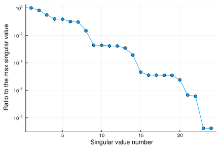
Figure 3: Ratio $\sigma_{i}/\sigma_{\max}$ for the singular values of $M^{*}$ (on a logarithmic scale).

Let us set the privacy parameters to $\delta=0.02$ and $\epsilon=\ln(3)$ for example (and $\rho_{i}$ to $\sqrt{3}$ as discussed above). We design the two-stage architecture of Figure 2 by first solving the stationary optimization problem (25a)-(25d), which provides an optimal matrix $\Pi^{*}$. Recall that the matrix $D$ can be then obtained from the factorization (19). The number of rows $q$ of $D$ is then equal to the rank of the matrix $M^{*}:=\kappa_{\delta,\epsilon}^{2}\left[\left(V-V\Pi^{*}V\right)^{-1}-V^{-1}\right]$. Due to the numerical procedures, this rank will typically be maximal (here equal to $24$). However, we plot on Fig. 3 the ratios $\sigma_{i}/\sigma_{\max}$ of the singular values of $M^{*}$, with $\sigma_{\max}$ the maximum singular value. We see that if we select for example only the singular values $\sigma_{i}\geq 10^{-4}\sigma_{\max}$ in the SVD of $M^{*}$ and set the smaller ones manually to $0$, we obtain a matrix of rank $14$, hence a matrix $D$ with $14$ rows instead of $24$. We then verify (by solving an algebraic Riccati equation) that the performance of the steady-state Kalman filter is left virtually unchanged by this truncation, with a steady-state MSE of about $160$, i.e., a root mean square error (RMSE) of $12.65$ for the estimate of the number $I_{t}$ of infectious people. In contrast, the input perturbation mechanism (i.e., taking $D=I$) gives a steady-state MSE of $777$ or RMSE on $I_{t}$ of $27.87$. Reducing the number of rows of $D$ is also beneficial for example in terms of processing complexity of the Kalman filter, which now has fewer inputs.

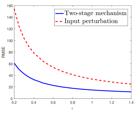
Figure 4: Steady-state RMSE of the total infectious population estimate for the two-stage and input perturbation mechanisms, as a function of the privacy parameter $\epsilon$ (here $\delta=0.01$).

For $\delta=0.01$, we compare on Fig. 4 the steady-state RMSE of the two-stage mechanism and the input perturbation architecture for different values of the privacy parameter $\epsilon$. One can see that by aggregating the input signals, we obtain a much better performance, especially in the high-privacy regime (when $\epsilon$ is small). Other measures of performance could also be of interest for the final filtering architecture, such as the convergence time of the estimates. For illustration purposes, Fig. 5 shows sample paths of differentially private estimates both for the two-stage mechanism and for the input perturbation mechanism.

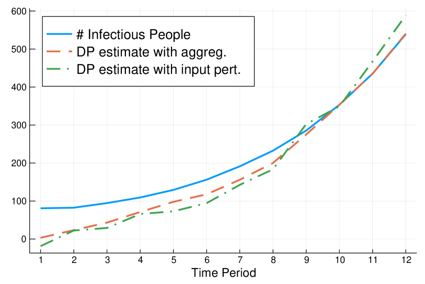
Figure 5: Sample paths of differentially private estimates (with $\delta=0.01,\;\epsilon=\ln(3)$) of the total infectious population, for the two-stage and input perturbation mechanisms. Both estimates are initialized with $\bar{x}_{0}=0$ and we show here the values after the measurement update step of the Kalman filter.

IV Differentially Private LQG Control

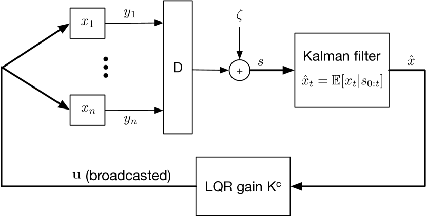
Figure 6: Differentially private LQG control architecture with first-stage signal aggregation.

We now turn to the LQG control problem introduced at the end of Section II-A. For concreteness, we assume here that the control input $u_{t}$ at time $t$ can depend on the measurements $y_{0:t}$ up to time $t$. It is straightforward to adapt the discussion to the case where only $y_{0:t-1}$ are available to compute $u_{t}$. By the separation principle [43, Chapter 8] for the standard LQG control problem (i.e., with no privacy constraint), the optimal control law for the system (2)-(3) and quadratic cost (5) is of the form $u_{t}=K^{c}_{t}\hat{x}_{t}$, where: i) $\hat{x}_{t}=\mathbb{E}[x_{t}|y_{0:t}]$ is the MMSE estimator, computed by the Kalman filter (14) independently of the design of the optimal control law; and ii) $K^{c}_{t}$ is the optimal gain for the deterministic linear quadratic regulator (LQR) problem, i.e., assuming that $w=0$ in (2) and $C=I_{n}$, $v=0$ in (3). In particular, since the sequence of control gains $K^{c}_{t}$ can be precomputed, the LQG control problem is similar to the filtering problem considered in the previous section, with the desired published output $\hat{z}_{t}=L_{t}\hat{x}_{t}$ simply replaced by $u_{t}=K^{c}_{t}\hat{x}_{t}$. This motivates the architecture proposed on Figure 6 for differentially private LQG control, which, compared to Figure 1(b), aggregates the measured signals $y_{i}$ before adding the privacy-preserving noise. Essentially, the only difference with the Kalman filtering problem is that the performance is measured by (5) instead of the MSE (4), so that the cost function in the optimization problem for the matrix $D$ needs to be changed. The following theorem summarizes the discussion above and the classical results (see for example [43, Chapter 8]) that allow us to formulate in the following an efficiently solvable optimization problem for the choice of aggregation matrix $D$ on Figure 6.

Theorem 4.

Given a choice of matrix $D$ for the differentially private LQG control architecture of Figure 6, the control law $u_{t}(y_{0:t})$, $t\geq 0$, minimizing the cost function (5) takes the form

$$u_{t}=K^{c}_{t}\hat{x}_{t},$$

where $\hat{x}_{t}$ is computed by the Kalman filter (14) and the gains $K^{c}_{t}$ are precomputed independently of the filtering problem as

$$K^{c}_{t}:=-(R_{t}+B_{t}^{T}P_{t+1}B_{t})^{-1}B_{t}^{T}P_{t+1}A_{t}$$

with the matrices $P_{t}\succeq 0$ given by $P_{T}=Q_{T}$ and the backward Riccati difference equation

$$P_{t}= A_{t}^{T}P_{t+1}A_{t}+Q_{t}$$

$$-A_{t}P_{t+1}B_{t}(R_{t}+B_{t}^{T}P_{t+1}B_{t})^{-1}B_{t}^{T}P_{t+1}A_{t}.$$ (30)

Moreover, the optimal objective (5) corresponding to this control law can be written

$$J_{T}=J^{c}_{T}+J^{f}_{T}(D)$$ (31)

where

$$J^{c}_{T}=\frac{1}{T+1}\left(\bar{x}_{0}^{T}P_{0}\bar{x}_{0}+\textup{Tr}(P_{0}\bar{\Sigma}_{0})+\sum_{t=1}^{T}\textup{Tr}(P_{t}W_{t})\right)$$

is a term independent of $D$ and

$$J_{T}^{f}(D) =\frac{1}{T+1}\sum_{t=0}^{T-1}\textup{Tr}(N_{t}\Sigma_{t}),\;\;\text{ with }$$ (32)

$$N_{t} =Q_{t}+A_{t}^{T}P_{t+1}A_{t}-P_{t},\;\;0\leq t\leq T-1,$$ (33)

and the matrices $\Sigma_{t}$ for $0\leq t\leq T-1$ defined by (15b)-(15d).

Note that the dependence on $D$ in (32) is due to the fact that the error covariance matrices $\Sigma_{t}$ depend on $D$ via (15b)-(15d). Moreover, from (30) we see that $N_{t}$ defined in (33) is positive semidefinite. Hence, we can define for all $0\leq t\leq T-1$ matrices $L_{t}$ such that $N_{t}=L_{t}^{T}L_{t}$, and $L_{T}=0$, to rewrite the cost (32) as $\frac{1}{T+1}\sum_{t=0}^{T}\textup{Tr}(L_{t}\Sigma_{t}L_{t}^{T})$. Minimizing this cost over the matrices $D$ with the relations (15b)-(15d) leads to an optimal aggregation matrix $D$ for the architecture of Figure 6. The reformulation of this optimization problem as an SDP then follows exactly from the same argument as in Section III-B2, which led to Theorem 2. In other words, we have the following result.

Proposition 1.

Let $L_{t}$, $0\leq t\leq T-1,$ be any matrices obtained from the factorization

$$L_{t}^{T}L_{t}=N_{t},0\leq t\leq T-1,$$

with $N_{t}$ defined by (33), and let $L_{T}=0$. Let $\Pi^{*}\succeq 0$,$\{X^{*}_{t}\succeq 0,\Omega^{*}_{t}\succ 0\}_{0\leq t\leq T}$ be an optimal solution for (23a)-(23e) with this choice of matrices $L_{t}$. Suppose that for some $0\leq t\leq T$, we have $L_{t}(\Omega^{*}_{t})^{-1}C_{t}^{T}\neq 0$. Let $D^{*}$ be a matrix obtained from $\Pi^{*}$ by the factorization (19). Then $D^{*}$ minimizes the LQG cost (5) among all the aggregation matrices $D$ of Figure 6. This cost is equal to $J_{T}^{c}+\frac{1}{T+1}\sum_{t=0}^{T}\textup{Tr}(X_{t}^{*})$, with $J_{T}^{c}$ defined in (31).

IV-A Stationary Problem

As in Section III-C for the filtering problem, we can consider the steady-state LQG problem by letting $T\to\infty$ and assuming the model (2)-(3) and the weight matrices $Q$ and $R$ in the cost (5) to be time-invariant. We assume the model to be detectable and stabilizable and the pair $(A,Q^{1/2})$ to be detectable, in order to be able to implement a stabilizing LQG controller. We can take the optimal gains $K^{c}$ and $K^{f}$ of the controller and the Kalman filter respectively to be also independent of time. Following Theorem 3 and Proposition 1, we then immediately have the following result for the design of the optimal $D$ matrix.

Proposition 2.

Let $P$ be the positive semidefinite solution of the following algebraic Riccati equation

$$P= A^{T}PA+Q-A^{T}PB(R+B^{T}PB)^{-1}B^{T}PA.$$

Let $L$ be any matrix obtained from the factorization

$$L^{T}L=A^{T}PA+Q-P.$$

Let $\Pi^{*}\succeq 0$, $X^{*}\succeq 0$, $\Omega^{*}\succ 0$ be an optimal solution for (25a)-(25d), for this choice of matrix $L$. Suppose that we have $L(\Omega^{*})^{-1}C^{T}\neq 0$. Let $D^{*}$ be a matrix obtained from $\Pi^{*}$ by the factorization (19). Then $D^{*}$ minimizes the steady-state LQG cost $J_{\infty}$ among all possible matrices $D$ introduced as in Figure 6, the corresponding value of the cost is $J_{\infty}=\textup{Tr}(PW)+\textup{Tr}(X^{*})$.

IV-B Numerical Simulations

We illustrate the above results numerically for $n=10$ independent scalar systems, with states $x_{i,t}$ evolving as first order systems with time-invariant dynamics (1), where

$$A_{1} =1.1,A_{2}=0.85,A_{3}=0.84,A_{4}=0.7,A_{5}=0.75,$$

$$A_{6} =0.9,A_{7}=0.8,A_{8}=1.05,A_{9}=0.99,A_{10}=1,$$

$C_{i}=1$, $W_{i}=0.02$ and $V_{i}=0.1$ for all $1\leq i\leq 10$, and $B$ is a $10\times 3$ matrix with $B_{ij}=0$ except for

$$B_{3,1} =B_{6,1}=B_{9,1}=1$$

$$B_{1,2} =B_{4,2}=B_{7,2}=B_{10,2}=1$$

$$B_{2,3} =B_{5,3}=B_{8,3}=1.$$

In other words, the published control signal is $3$-dimensional, with control input $u_{1}$ simultaneously actuating systems $3,6,9$, $u_{2}$ actuating systems $1,4,7,10$ and $u_{3}$ actuating systems $2,5$ and $8$. We wish to regulate the sum of the states $\sum_{i=1}^{10}x_{i}$ to $0$, hence we take $Q$ to be the $10\times 10$ all-ones matrix and $R=I_{3}$ in (5). We set the privacy parameters to $\delta=0.05$ and $\epsilon=\ln(3)$, and $\rho_{i}=1$ for $1\leq i\leq 10$.

To design the differentially private LQG controller with signal aggregation for the stationary problem, we compute the matrix $L$ of Proposition 2 and solve the optimization problem (25a)-(25d). Following the methodology discussed at the end of Section III-D, we find that one can take the matrix $D$ to be a $4\times 10$ matrix at the matrix factorization stage (19). The corresponding steady-state cost $J_{\infty}$ is found to be $1.37$, whereas it is $2.17$ for the input perturbation mechanism (i.e., with $D=I_{10}$). Hence, signal aggregation results in a significant improvement. Figure 7 shows a comparison of the cost $J_{\infty}$ for this problem, with the two architectures, for different values of $\epsilon$. Finally, Figure 8 illustrates the sample paths obtained under closed-loop control with the differentially private controllers. We see in particular on Figure 8(b) that the two-stage architecture provides a much better transient behavior for the regulated average trajectory (or sum of trajectories) compared to the input perturbation architecture, in addition to a better steady-state performance.

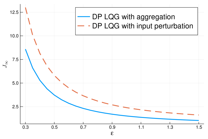
Figure 7: Optimal steady-state quadratic cost $J_{\infty}$ as a function of the privacy parameter $\epsilon$, for the architecture with signal aggregation and for the input perturbation mechanism. Here $\delta=0.05$.

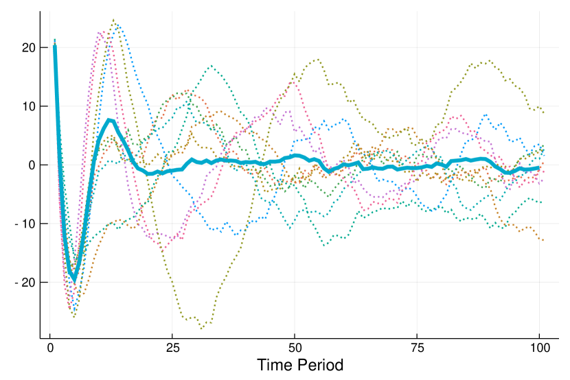
(a) Sample paths for the individual trajectories and the regulated average trajectory ($\frac{1}{10}\sum_{i=1}^{10}x_{i,t}$, thick solid line) using the LQG controller with signal aggregation.

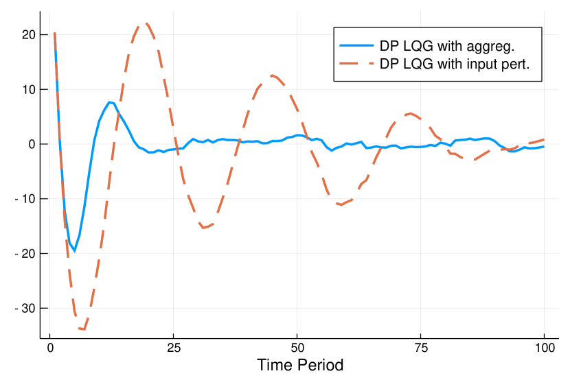
(b) Sample paths of the regulated average trajectories for the LQG controllers with input perturbation and signal aggregation.

Figure 8: Individual and average trajectories under differentially private closed-loop control. Here $\epsilon=\ln(3),\delta=0.05$. All individual system states start in the neighborhood of $20$, which is also the value used to initialize the Kalman filter estimates for all states.

V Conclusion

This paper considers the Kalman filtering and LQG optimal control problems under a differential privacy constraint. We propose an architecture combining an input stage aggregating the individual signals appropriately, the Gaussian mechanism to enforce differential privacy and a Kalman filter to reconstruct the desired estimate. Optimizing the parameters of this architecture can be recast as an SDP. Examples illustrate the performance improvements compared to the input perturbation mechanism, which adds noise directly on the individual signals. The methodology is then adapted to propose a similar two-stage architecture for an LQG control problem, where the goal is to compute a shared control broadcasted to the agent population. Future research could consider the extension of these ideas to nonlinear systems, improving on the input and output perturbation mechanisms of [23]. In addition, since the size of the SDP increases rapidly with the number of agents (and the time horizon in the non-stationary case), it would be useful to develop numerical methods and a problem-specific solver that take advantage of the sparsity of the matrices involved in the constraints, as in [44] for example.

References

- [1] K. H. Degue and J. Le Ny, “On differentially private Kalman filtering,” in Proceedings of the 5th IEEE Global Conference on Signal and Information Processing (GlobalSIP), Montreal, Canada, Nov. 2017.
- [2] J. C. Herrera, D. B. Work, R. Herring, X. Ban, Q. Jacobson, and A. M. Bayen, “Evaluation of traffic data obtained via GPS-enabled mobile phones: The Mobile Century field experiment,” Transportation Research Part C: Emerging Technologies, vol. 18, no. 4, pp. 568 – 583, 2010.
- [3] R. Shokri, G. Theodorakopoulos, J. Y. Le Boudec, and J. P. Hubaux, “Quantifying location privacy,” in Proceedings of the IEEE Symposium on Security and Privacy, Oakland, California, May 2011, pp. 247–262.
- [4] Y.-A. de Montjoye, C. A. Hidalgo, M. Verleysen, and V. D. Blondel, “Unique in the crowd: The privacy bounds of human mobility,” Scientific Reports, vol. 3, 2013.
- [5] F. Xu, Z. Tu, Y. Li, P. Zhang, X. Fu, and D. Jin, “Trajectory recovery from ash: User privacy is not preserved in aggregated mobility data,” in Proceedings of the 26th International Conference on World Wide Web, 2017, pp. 1241–1250.
- [6] A. Pyrgelis, C. Troncoso, and E. D. Cristofaro, “What does the crowd say about you? evaluating aggregation-based location privacy,” Proceedings on Privacy Enhancing Technologies, vol. 4, pp. 156–176, 2017.
- [7] G. W. Hart, “Nonintrusive appliance load monitoring,” Proceedings of the IEEE, vol. 80, no. 12, pp. 1870–1891, December 1992.
- [8] G. Bauer, K. Stockinger, and P. Lukowicz, “Recognizing the use-mode of kitchen appliances from their current consumption,” EuroSSC, pp. 163–176, 2009.
- [9] M. A. Lisovich, D. K. Mulligan, and S. B. Wicker, “Inferring personal information from demand-response systems,” IEEE Security and Privacy, vol. 8, no. 1, pp. 11–20, 2010.
- [10] A. Molina-Markham, P. Shenoy, K. Fu, E. Cecchet, and D. Irwin, “Private memoirs of a smart meter,” in Proceedings of the 2nd ACM Workshop on Embedded Sensing Systems for Energy-Efficiency in Building, New York, NY, USA, 2010, pp. 61–66.
- [11] L. Sankar, S. Raj Rajagopalan, and V. H. Poor, “Utility-privacy tradeoffs in databases: An information-theoretic approach,” IEEE Transactions on Information Forensics and Security, vol. 8, no. 6, pp. 838–852, June 2013.
- [12] F. Farokhi and H. Sandberg, “Fisher information privacy with application to smart meter privacy using HVAC units,” in Privacy in Dynamical Systems, F. Farokhi, Ed. Springer, 2020, pp. 3–17.
- [13] Y. Mo and R. M. Murray, “Privacy preserving average consensus,” IEEE Transactions on Automatic Control, vol. 62, no. 2, pp. 753–765, 2016.
- [14] Y. Song, C. X. Wang, and W. P. Tay, “Compressive privacy for a linear dynamical system,” IEEE Trans. Inf. Forensics Security, vol. 15, pp. 895 – 910, 2020.
- [15] F. Fei, S. Li, H. Dai, C. Hu, W. Dou, and Q. Ni, “A k-anonymity based schema for location privacy preservation,” IEEE Transactions on Sustainable Computing, vol. 4, no. 2, pp. 156–167, Apr. 2019.
- [16] C. Dwork, F. McSherry, K. Nissim, and A. Smith, “Calibrating noise to sensitivity in private data analysis,” in Proceedings of the Third Theory of Cryptography Conference, 2006, pp. 265–284.
- [17] C. Dwork, “Differential privacy,” in Proceedings of the 33rd International Colloquium on Automata, Languages and Programming (ICALP), ser. Lecture Notes in Computer Science, vol. 4052. Springer-Verlag, 2006.
- [18] C. Dwork and A. Roth, “The algorithmic foundations of differential privacy,” Foundations and Trends in Theoretical Computer Science, vol. 9, no. 3-4, pp. 211–407, August 2014.
- [19] C. Dwork, M. Naor, T. Pitassi, and G. N. Rothblum, “Differential privacy under continual observations,” in Proceedings of the ACM Symposium on the Theory of Computing (STOC), Cambridge, MA, June 2010.
- [20] L. Fan and L. Xiong, “An adaptive approach to real-time aggregate monitoring with differential privacy,” IEEE Transactions on knowledge and data engineering, vol. 26, no. 9, pp. 2094–2106, 2014.
- [21] J. Le Ny and G. J. Pappas, “Differential private filtering,” IEEE Transactions on Automatic Control, vol. 59, no. 2, pp. 341–354, February 2014.
- [22] J. Le Ny and M. Mohammady, “Differentially private MIMO filtering for event streams,” IEEE Transactions on Automatic Control, vol. 63, no. 1, 01 2018.
- [23] J. Le Ny, “Differentially private nonlinear observer design using contraction analysis,” International Journal of Robust and Nonlinear Control, 2018. [Online]. Available: https://onlinelibrary.wiley.com/doi/abs/10.1002/rnc.4392
- [24] A. McGlinchey and O. Mason, “Bounding the sensitivity for positive linear observers,” in European Control Conference (ECC), 2018, pp. 1214–1219.
- [25] Y. Wang, Z. Huang, S. Mitra, and G. E. Dullerud, “Differential privacy in linear distributed control systems: Entropy minimizing mechanisms and performance tradeoffs,” IEEE Transactions on Control of Network Systems, vol. 4, no. 1, pp. 118–130, Mar. 2017.
- [26] M. T. Hale, A. Jones, and K. Leahy, “Privacy in feedback: The differentially private LQG,” in Proceedings of the American Control Conference (ACC), Milwaukee, WI, USA, Jun. 2018.
- [27] Z. Huang, S. Mitra, and G. Dullerud, “Differentially private iterative synchronous consensus,” in Proceedings of the ACM Workshop on Privacy in the Electronic Society, 2012, pp. 81––90.
- [28] E. Nozari, P. Tallapragada, and J. Cortés, “Differentially private average consensus: Obstructions, trade-offs, and optimal algorithm design,” Automatica, vol. 81, pp. 221–231, 2017.
- [29] R. Cummings, S. Krehbiel, Y. Mei, R. Tuo, and W. Zhang, “Differentially private change-point detection,” in Advances in Neural Information Processing Systems, 2018.
- [30] K. H. Degue and J. Le Ny, “On differentially private Gaussian hypothesis testing,” in Proceedings of the 56th Annual Allerton Conference on Communication, Control, and Computing, Allerton Park and Retreat Center, Monticello, Illinois, USA, Oct. 2018.
- [31] V. Rostampour, R. Ferrari, A. Teixeira, and T. Keviczky, “Differentially-private distributed fault diagnosis for large-scale nonlinear uncertain systems,” in IFAC Symposium on Fault Detection, Supervision and Safety for Technical Processes, 2018.
- [32] J. Le Ny, E. Feron, and M. Dahleh, “Scheduling continuous-time Kalman filters,” IEEE Transactions on Automatic Control, vol. 56, no. 6, June 2011.
- [33] A. I. Mourikis and S. I. Roumeliotis, “Optimal sensor scheduling for resource-constrained localization of mobile robot formations,” IEEE Transactions on Robotics, vol. 22, no. 5, pp. 917–931, 2006.
- [34] T. Tanaka, K.-K. K. Kim, P. A. Parrilo, and S. Mitter, “Semidefinite programming approach to Gaussian sequential rate-distortion trade-offs,” IEEE Transactions on Automatic Control, vol. 62, no. 4, pp. 1896–1910, April 2017.
- [35] B. D. O. Anderson and J. B. Moore, Optimal filtering. New York, NY, USA: Dover: Dover, 2005.
- [36] C. Dwork, K. Kenthapadi, F. McSherry, I. Mironov, and M. Naor, “Our data, ourselves: Privacy via distributed noise generation,” Advances in Cryptology-EUROCRYPT, vol. 4004, pp. 486–503, 2006.
- [37] J. Le Ny and G. J. Pappas, “Differentially private Kalman filtering,” in Proceedings of the 50th Annual Allerton Conference, Allerton House, UIUC, Illinois, USA, October 2012.
- [38] S. Boyd, L. El Ghaoui, E. Feron, and V. Balakrishnan, Linear matrix Inequalities in system and control theory. SIAM, 1994, vol. 15.
- [39] V. Dukic, H. F. Lopes, and N. G. Polson, “Tracking epidemics with Google flu trends data and a state-space SEIR model,” Journal of the American Statistical Association, vol. 107, no. 500, pp. 1410–1426, 2012.
- [40] K. H. Degue and J. Le Ny, “Estimation and outbreak detection with interval observers for uncertain discrete-time SEIR epidemic models,” International Journal of Control, pp. 1–12, 2019. [Online]. Available: https://doi.org/10.1080/00207179.2019.1643492
- [41] H. W. Hethcote, “The mathematics of infectious diseases,” SIAM Review, vol. 42, no. 4, pp. 599–653, 2000.
- [42] Z. Hu, Z. Teng, and H. Jiang, “Stability analysis in a class of discrete SIRS epidemic models,” Nonlinear Analysis: Real World Applications, vol. 13, no. 5, pp. 2017–2033, 2012.
- [43] K. J. Åström, Introduction to stochastic control theory. Academic Press, 1970.
- [44] S. Benson, Y. Ye, and X. Zhang, “Solving large-scale sparse semidefinite programs for combinatorial optimization,” SIAM Journal on Optimization, vol. 10, no. 2, pp. 443–461, 2000.