Structure and decays of nuclear three-body systems: the Gamow coupled-channel method in Jacobi coordinates

Abstract

Background

Weakly bound and unbound nuclear states appearing around particle thresholds are prototypical open quantum systems. Theories of such states must take into account configuration mixing effects in the presence of strong coupling to the particle continuum space.

Purpose

To describe structure and decays of three-body systems, we developed a Gamow coupled-channel (GCC) approach in Jacobi coordinates by employing the complex-momentum formalism. We benchmarked the new framework against the complex-energy Gamow Shell Model (GSM).

Methods

The GCC formalism is expressed in Jacobi coordinates, so that the center-of-mass motion is automatically eliminated. To solve the coupled-channel equations, we use hyperspherical harmonics to describe the angular wave functions while the radial wave functions are expanded in the Berggren ensemble, which includes bound, scattering and Gamow states.

Results

We show that the GCC method is both accurate and robust. Its results for energies, decay widths, and nucleon-nucleon angular correlations are in good agreement with the GSM results.

Conclusions

We have demonstrated that a three-body GSM formalism explicitly constructed in cluster-orbital shell model coordinates provides similar results to a GCC framework expressed in Jacobi coordinates, provided that a large configuration space is employed. Our calculations for $A=6$ systems and ²⁶O show that nucleon-nucleon angular correlations are sensitive to the valence-neutron interaction. The new GCC technique has many attractive features when applied to bound and unbound states of three-body systems: it is precise, efficient, and can be extended by introducing a microscopic model of the core.

I Introduction

Properties of rare isotopes that inhabit remote regions of the nuclear landscape at and beyond the particle driplines are in the forefront of nuclear structure and reaction research Dobaczewski and Nazarewicz (1998); RIS (2007); Dobaczewski et al. (2007); Forssén et al. (2013); Balantekin et al. (2014); NSA (2015). The next-generation of rare isotope beam facilities will provide unique data on dripline systems that will test theory, highlight shortcomings, and identify areas for improvement. The challenge for nuclear theory is to develop methodologies to reliably calculate and understand the properties and dynamics of new physical systems with different properties due to large neutron-to-proton asymmetries and low-lying reaction thresholds. Here, dripline systems are of particular interest as they can exhibit exotic radioactive decay modes such as two-nucleon emission Pfützner et al. (2012); Pfützner (2013); Thoennessen (2004); Blank and Płoszajczak (2008); Grigorenko et al. (2011); Olsen et al. (2013); Kohley et al. (2013). Theories of such nuclei must take into account their open quantum nature.

Theoretically, a powerful suite of $A$-body approaches based on inter-nucleon interactions provides a quantitative description of light and medium-mass nuclei and their reactions Elhatisari et al. (2015); Navrátil et al. (2016); Kumar et al. (2017). To unify nuclear bound states with resonances and scattering continuum within one consistent framework, advanced continuum shell-model approaches have been introduced Michel et al. (2009); Hagen et al. (2012); Papadimitriou et al. (2013). Microscopic models of exotic nuclear states have been supplemented by a suite of powerful, albeit more phenomenological models, based on effective degrees of freedom such as cluster structures. While such models provide a “lower resolution” picture of the nucleus, they can be extremely useful when interpreting experimental data, providing guidance for future measurements, and provide guidance for more microscopic approaches.

The objective of this work is to develop a new three-body method to describe both reaction and structure aspects of two-particle emission. A prototype system of interest is the two-neutron-unbound ground state of ²⁶O Lunderberg et al. (2012); Kohley et al. (2013); Kondo et al. (2016). According to theory, ²⁶O exhibits the dineutron-type correlations Grigorenko and Zhukov (2015); Kondo et al. (2016); Hagino and Sagawa (2016a, b); Fossez et al. (2017). To describe such a system, nuclear model should be based on a fine-tuned interaction capable of describing particle-emission thresholds, a sound many-body method, and a capability to treat simultaneously bound and unbound states.

If one considers bound three-body systems, few-body models are very useful Braaten and Hammer (2006), especially models based on the Lagrange-mesh technique Baye et al. (1994) or cluster-orbital shell model (COSM) Suzuki and Ikeda (1988). However, for the description of resonances, the outgoing wave function in the asymptotic region need to be treated very carefully. For example, one can divide the coordinate space into internal and asymptotic regions, where the R-matrix theory Descouvemont et al. (2006); Lovell et al. (2017), microscopic cluster model Damman and Descouvemont (2009), and the diagonalization of the Coulomb interaction Grigorenko et al. (2009a) can be used. Other useful techniques include the Green function method Hagino and Sagawa (2016a) and the complex scaling Aoyama et al. (2006); Kruppa et al. (2014).

Our strategy is to construct a precise three-body framework to weakly bound and unbound systems similar to that of the GSM Michel et al. (2002). The attractive feature of the GSM is that – by employing the Berggren ensemble Berggren (1968) – it treats bound, scattering, and outgoing Gamow states on the same footing. Consequently, energies and decay widths are obtained simultaneously as the real and imaginary parts of the complex eigenenergies of the shell model Hamiltonian Michel et al. (2009). In this study, we develop a three-body Gamow coupled-channel (GCC) approach in Jacobi coordinates with the Berggren basis. Since the Jacobi coordinates allow for the exact treatment of nuclear wave functions in both nuclear and asymptotic regions, and as the Berggren basis explicitly takes into account continuum effects, a comprehensive description of weakly-bound three-body systems can be achieved. As the GSM is based on the COSM coordinates, a recoil term appears due to the center-of-mass motion. Hence, it is of interest to compare Jacobi- and COSM-based frameworks for the description of weakly bound and resonant nuclear states.

This article is organized as follows. Section II contains the description of models and approximations. In particular, it lays out the new GCC approach and GSM model used for benchmarking, and defines the configuration spaces used. The results for $A=6$ systems and ²⁶O are contained in Sec. III. Finally, the summary and outlook are given in Sec. IV.

II The Model

II.1 Gamow Coupled Channel approach

In the three-body GCC model, the nucleus is described in terms of a core and two valence nucleons (or clusters). The GCC Hamiltonian can be written as:

$$\hat{H}=\sum^{3}_{i=1}\frac{\hat{\mbox{\boldmath$p$}}^{2}_{i}}{2m_{i}}+\sum^{3}_{i>j=1}V_{ij}(\mbox{\boldmath$r$}_{ij})-\hat{T}_{\rm c.m.},$$ (1)

where $V_{ij}$ is the interaction between clusters $i$ and $j$, including central, spin-orbit and Coulomb terms, and $\hat{T}_{\rm c.m.}$ stands for the kinetic energy of the center-of-mass.

The unwanted feature of three-body models is the appearance of Pauli forbidden states arising from the lack of antisymmetrization between core and valence particles. In order to eliminate the Pauli forbidden states, we implemented the orthogonal projection method Saito (1969); Kukulin and Pomerantsev (1978); Descouvemont et al. (2003) by adding to the GCC Hamiltionan the Pauli operator

$$\hat{Q}=\Lambda\sum_{c}|\varphi^{j_{c}m_{c}}\rangle\langle\varphi^{j_{c}m_{c}}|,$$ (2)

where $\Lambda$ is a constant and $|\varphi^{j_{c}m_{c}}\rangle$ is a 2-body state involving forbidden s.p. states of core nucleons. At large values of $\Lambda$, Pauli-forbidden states appear at high energies, so that they are effectively suppressed.

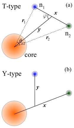
Figure 1: Jacobi coordinates in a three-body system.

In order to describe three-body asymptotics and to eliminate the spurious center-of-mass motion exactly, we express the GCC model in the relative (Jacobi) coordinates Navrátil et al. (2000); Descouvemont et al. (2003); Navrátil et al. (2016); Lovell et al. (2017):

$$\mbox{\boldmath$x$} =\sqrt{\mu_{ij}}(\mbox{\boldmath$r$}_{i}-\mbox{\boldmath$r$}_{j}),$$ (3)

$$\mbox{\boldmath$y$} =\sqrt{\mu_{(ij)k}}\left(\mbox{\boldmath$r$}_{k}-\frac{A_{i}\mbox{\boldmath$r$}_{i}+A_{j}\mbox{\boldmath$r$}_{j}}{A_{i}+A_{j}}\right),$$

where $\mbox{\boldmath$r$}_{i}$ is the position vector of the i-th cluster, $A_{i}$ is the i-th cluster mass number, and $\mu_{ij}$ and $\mu_{(ij)k}$ are the reduced masses associated with $x$ and $y$, respectively:

$$\mu_{ij} =\frac{A_{i}A_{j}}{A_{i}+A_{j}},$$ (4)

$$\mu_{(ij)k} =\frac{(A_{i}+A_{j})A_{k}}{A_{i}+A_{j}+A_{k}}.$$

As one can see in Fig. 1, Jacobi coordinates can be expressed as T- and Y-types, each associated with a complete basis set. In practice, it is convenient to calculate the matrix elements of the two-body interaction individually in T- and Y-type coordinates, and then transform them to one single Jacobi set. To describe the transformation between different types of Jacobi coordinates, it is convenient to introduce the basis of hyperspherical harmonics (HH) Fabre de la Ripelle (1983); Kievsky et al. (2008). The hyperspherical coordinates are constructed from a five-dimensional hyperangular coordinates $\Omega_{5}$ and a hyperradial coordinate $\rho=\sqrt{x^{2}+y^{2}}$. The transformation between different sets of Jacobi coordinates is given by the Raynal-Revai coefficients Raynal and Revai (1970).

Expressed in HH, the total wave-function can be written as Descouvemont et al. (2003):

$$\Psi^{JM\pi}(\rho,\Omega_{5})=\rho^{-5/2}\sum_{\gamma K}\psi^{J\pi}_{\gamma K}(\rho)\mathcal{Y}^{JM}_{\gamma K}(\Omega_{5}),$$ (5)

where $K$ is the hyperspherical quantum number and $\gamma=\{s_{1},s_{2},s_{3},S_{12},S,\ell_{x},\ell_{y},L\}$ is a set of quantum numbers other than $K$. The quantum numbers $s$ and $\ell$ stand for spin and orbital angular momentum, respectively, $\psi^{J\pi}_{\gamma K}(\rho)$ is the hyperradial wave function, and $\mathcal{Y}^{JM}_{\gamma K}(\Omega_{5})$ is the hyperspherical harmonic.

The resulting Schrödinger equation for the hyperradial wave functions can be written as a set of coupled-channel equations:

$$\left[-\frac{\hbar^{2}}{2m}\left(\frac{d^{2}}{d\rho^{2}}-\frac{(K+3/2)(K+5/2)}{\rho^{2}}\right)-\tilde{E}\right]\psi^{J\pi}_{\gamma K}(\rho)$$ (6)

$$+\sum_{K^{\prime}\gamma^{\prime}}V^{J\pi}_{K^{\prime}\gamma^{\prime},K\gamma}(\rho)\psi^{J\pi}_{\gamma^{\prime}K^{\prime}}(\rho) +\sum_{K^{\prime}\gamma^{\prime}}\int_{0}^{\infty}W_{K^{\prime}\gamma^{\prime},K\gamma}(\rho,\rho^{\prime})\psi^{L\pi}_{\gamma^{\prime}K^{\prime}}(\rho^{\prime})d\rho^{\prime}=0,$$

where

$$V^{L\pi}_{K^{\prime}\gamma^{\prime},K\gamma}(\rho)=\langle\mathcal{Y}^{JM}_{\gamma^{\prime}K^{\prime}}|\sum^{3}_{i>j=1}V_{ij}(\mbox{\boldmath$r$}_{ij})|\mathcal{Y}^{JM}_{\gamma K}\rangle$$ (7)

and

$$W_{K^{\prime}\gamma^{\prime},K\gamma}(\rho,\rho^{\prime})=\langle\mathcal{Y}^{JM}_{\gamma^{\prime}K^{\prime}}|\hat{Q}|\mathcal{Y}^{JM}_{\gamma K}\rangle$$ (8)

is the non-local potential generated by the Pauli projection operator (2).

In order to treat the positive-energy continuum space precisely, we use the Berggren expansion technique for the hyperradial wave function:

$$\psi^{J\pi}_{\gamma K}(\rho)=\sum_{\rm n}C^{J\pi M}_{\gamma{\rm n}K}\mathcal{B}^{J\pi}_{\gamma{\rm n}}(\rho),$$ (9)

where $\mathcal{B}^{J\pi}_{\gamma{\rm n}}(\rho)$ represents a s.p. state belonging to to the Berggren ensemble Berggren (1968). The Berggren ensemble defines a basis in the complex momentum plane, which includes bound, decaying, and scattering states. The completeness relation for the Berggren ensemble can be written as:

$$\sum_{{\rm n}\in b,d}\mathcal{B}_{\rm n}(k_{\rm n},\rho)\mathcal{B}_{\rm n}(k_{\rm n},\rho^{\prime})+ \int_{L^{+}}\mathcal{B}(k,\rho)\mathcal{B}(k,\rho^{\prime})dk$$ (10)

$$=\delta(\rho-\rho^{\prime}),$$

where $b$ are bound states and $d$ are decaying resonant (or Gamow) states lying between the real-$k$ momentum axis in the fourth quadrant of the complex-$k$ plane, and the $L^{+}$ contour representing the complex-$k$ scattering continuum. For numerical purposes, ${L^{+}}$ has to be discretized, e.g., by adopting the Gauss-Legendre quadrature Hagen et al. (2006). In principle, the contour ${L^{+}}$ can be chosen arbitrarily as long as it encompasses the resonances of interest. If the contour $L^{+}$ is chosen to lie along the real $k$-axis, the Berggren completeness relation reduces to the Newton completeness relation Newton (1982) involving bound and real-momentum scattering states.

To calculate radial matrix elements with the Berggren basis, we employ the exterior complex scaling Gyarmati and Vertse (1971), where integrals are calculated along a complex radial path:

$$\langle\mathcal{B}_{\rm n}| V(\rho)|\mathcal{B}_{\rm m}\rangle=\int_{0}^{R}\mathcal{B}_{\rm n}(\rho)V(\rho)\mathcal{B}_{\rm m}(\rho)d\rho$$ (11)

$$+\int_{0}^{+\infty}\mathcal{B}_{\rm n}(R+\rho e^{i\theta})V(R+\rho e^{i\theta})\mathcal{B}_{\rm m}(R+\rho e^{i\theta})d\rho.$$

For potentials that decrease as $O(1/\rho^{2})$ (centrifugal potential) or faster (nuclear potential), $R$ should be sufficiently large to bypass all singularities and the scaling angle $\theta$ is chosen so that the integral converges, see Ref. Michel et al. (2003) for details. As the Coulomb potential is not square-integrable, its matrix elements diverge when $k_{n}=k_{m}$. A practical solution is provided by the so-called “off-diagonal method” proposed in Ref. Michel (2011). Basically, a small offset $\pm\delta k$ is added to the linear momenta $k_{n}$ and $k_{m}$ of involved scattering wave-functions, so that the resulting diagonal Coulomb matrix element converges.

II.2 Gamow Shell Model

In the GSM, expressed in COSM coordinates, one deals with the center-of-mass motion by adding a recoil term ($\hat{\mbox{\boldmath$p$}}_{1}\cdot\hat{\mbox{\boldmath$p$}}_{2}/m_{n}A_{\rm core}$) Suzuki and Ikeda (1988); Michel et al. (2002). The GSM Hamiltonian is diagonalized in a basis of Slater determinants built from the one-body Berggren ensemble. In this case, it is convenient to deal with the Pauli principle by eliminating spurious excitations at a level of the s.p. basis. In practice, one just needs to construct a valence s.p. space that does not contain the orbits occupied in the core. It is equivalent to the projection technique used in GCC wherein the Pauli operator (2) expressed in Jacobi coordinates has a two-body character. The treatment of the interactions is the same in GSM and GCC. In both cases, we use the complex scaling method to calculate matrix elements Michel et al. (2003) and the “off-diagonal method” to deal with the Coulomb potential Michel (2011).

The two-body recoil term is treated in GSM by expanding it in a truncated basis of harmonic oscillator (HO). The HO basis depends on the oscillator length $b$ and the number of states used in the expansion. As it was demonstrated in Refs. Hagen et al. (2006); Michel et al. (2010), GSM eigenvalues and eigenfunctions converge for a sufficient number of HO states, and the dependence of the results on $b$ is very weak.

Let us note in passing that one has to be careful when using arguments based on the variational principle when comparing the performance of GSM with GCC. Indeed, the treatment of the Pauli-forbidden states is slightly different in the two approaches. Moreover, the recoil effect in the GSM is not removed exactly. (There is no recoil term in GCC as the center-of-mass motion is eliminated through the use of Jacobi coordinates.)

II.3 Two-nucleon correlations

In order to study the correlations between the two valence nucleons, we utilize the two-nucleon density Bertsch and Esbensen (1991); Hagino and Sagawa (2005); Papadimitriou et al. (2011) $\rho_{nn^{\prime}}(r,r^{\prime},\theta)=\langle\Psi|\delta(r_{1}-r)\delta(r_{2}-r^{\prime})\delta(\theta_{12}-\theta)|\Psi\rangle$, where $r_{1}$, $r_{2}$, and $\theta_{12}$ are defined in Fig. 1(a). In the following, we apply the normalization convention of Ref. Papadimitriou et al. (2011) in which the Jacobian $8\pi^{2}r^{2}r^{\prime 2}\sin\theta$ is incorporated into the definition of $\rho_{nn^{\prime}}$, i.e., it does not appear explicitly. The angular density of the two valence nucleons is obtained by integrating $\rho_{nn^{\prime}}(r,r^{\prime},\theta)$ over radial coordinates:

$$\rho(\theta)=\int\rho_{nn^{\prime}}(r,r^{\prime},\theta)drdr^{\prime}.$$ (12)

The angular density is normalized to one: $\int\rho(\theta)d\theta=1.$

While it is straightforward to calculate $\rho_{nn^{\prime}}$ with COSM coordinates, the angular density cannot be calculated directly with the Jacobi T-type coordinates used to diagonalize the GCC Hamiltonian. Consequently, one can either calculate the density distribution $\rho_{\rm T}(x,y,\varphi)$ in T-type coordinates and then transform it to $\rho(r_{1},r_{2},\theta_{12})$ in COSM coordinates by using the geometric relations of Fig. 1(a), or – as we do in this study – one can apply the T-type-to-COSM coordinate transformation. This transformation Raynal and Revai (1970), provides an analytical relation between hyperspherical harmonics in COSM coordinates $\mathcal{Y}^{JM}_{\gamma^{\prime}K^{\prime}}(\mbox{\boldmath$r$}_{1}^{\prime},\mbox{\boldmath$r$}_{2}^{\prime})$ and the T-type Jacobi coordinates $\mathcal{Y}^{JM}_{\gamma K}(\mbox{\boldmath$x$}^{\prime},\mbox{\boldmath$y$}^{\prime})$, where $\mbox{\boldmath$r$}_{1}^{\prime}$, $\mbox{\boldmath$r$}_{2}^{\prime}$, $\mbox{\boldmath$x$}^{\prime}$ and $\mbox{\boldmath$y$}^{\prime}$ are:

$$\mbox{\boldmath$r$}_{1}^{\prime} =\sqrt{A_{i}}\mbox{\boldmath$r$}_{1},$$ (13)

$$\mbox{\boldmath$r$}_{2}^{\prime} =\sqrt{A_{j}}\mbox{\boldmath$r$}_{2},$$

$$\mbox{\boldmath$x$}^{\prime} =\mbox{\boldmath$x$}=\sqrt{\mu_{ij}}(\mbox{\boldmath$r$}_{1}-\mbox{\boldmath$r$}_{2}),$$

$$\mbox{\boldmath$y$}^{\prime} =\sqrt{\frac{A_{i}+A_{j}}{\mu_{(ij)k}}}\mbox{\boldmath$y$}=\frac{A_{i}\mbox{\boldmath$r$}_{1}+A_{j}\mbox{\boldmath$r$}_{2}}{\sqrt{A_{i}+A_{j}}}.$$

II.4 Model space and parameters

In order to compare approaches formulated in Jacobi and COSM coordinates, we consider model spaces defined by the cutoff value $\ell_{\rm max}$, which is the maximum orbital angular momentum associated with ($\mbox{\boldmath$r$}_{1}$, $\mbox{\boldmath$r$}_{2}$) in GSM and ($x$, $y$) in GCC. The remaining truncations come from the Berggren basis itself.

The nuclear two-body interaction between valence nucleons has been approximated by the finite-range Minnesota force with the original parameters of Ref. Thompson et al. (1977). For the core-valence Hamiltonian, we took a Woods-Saxon (WS) potential with parameters fitted to the resonances of the core+$n$ system. The one- and two-body Coulomb interaction has been considered when valence protons are present.

In the case of GSM, we use the Berggren basis for the $spd$ partial waves and a HO basis for the channels with higher orbital angular momenta. For ⁶He, ⁶Li and ⁶Be we assume the ⁴He core. For ⁶He and ⁶Be, GSM we took a complex-momentum contour defined by the segments $k=0\rightarrow 0.17-0.17i\rightarrow 0.34\rightarrow 3$ (all in  fm^-1) for the $p_{3/2}$ partial wave, and $0\rightarrow 0.5\rightarrow 1\rightarrow 3$ fm^-1 for the remaining $spd$ partial waves. For ⁶Li, we took the contours $0\rightarrow 0.18-0.17i\rightarrow 0.5\rightarrow 3$ fm^-1 for $p_{1/2}$; $0\rightarrow 0.15-0.14i\rightarrow 0.5\rightarrow 3$ fm^-1 for $p_{3/2}$; and $0\rightarrow 0.25\rightarrow 0.5\rightarrow 3$ fm^-1 for the $sd$ partial waves. Each segment was discretized with 10 points. This is sufficient for the energies and most of other physical quantities, but one may need more points to describe wave functions precisely, especially for the unbound resonant states that are affected by Coulomb interaction. Hence, we choose 15 points for each segment to calculate the two-proton angular correlation of the unbound ⁶Be. The HO basis was defined through the oscillator length $b=2$ fm and the maximum radial quantum number $n_{\rm max}=10$. The WS parameters for the $A=6$ nuclei are: the depth of the central term $V_{0}=47$ MeV; spin-orbit strength $V_{\rm s.o.}=30$ MeV; diffuseness $a=0.65$ fm; and the WS (and charge) radius $R=2$ fm. With these parameters we predict the $3/2^{-}$ ground state (g.s.) of ⁵He at $E=0.732$ MeV ($\Gamma=0.622$ MeV), and its first excited $1/2^{-}$ state at $E=2.126$ MeV ($\Gamma=5.838$ MeV).

For ²⁶O, we consider the ²⁴O core Kanungo et al. (2009); Hoffman et al. (2009); Hagino and Sagawa (2016a). In the GSM variant, we used the contour $0\rightarrow 0.2-0.15i\rightarrow 0.4\rightarrow 3$ fm^-1 for $d_{3/2}$, and $0\rightarrow 0.5\rightarrow 1\rightarrow 3$ fm^-1 for the remaining $spd$ partial waves. For the HO basis we took $b=1.75$ fm and $n_{\rm max}=10$. The WS potential for ²⁶O has fitted in Ref. Hagino and Sagawa (2016a) to the resonances of ²⁵O. Its parameters are: $V_{0}=44.1$ MeV, $V_{\rm s.o.}=45.87$ MeV, $a=0.73$ fm, and $R=3.6$ fm.

The GCC calculations have been carried out with the maximal hyperspherical quantum number $K_{\rm max}$ = 40, which is sufficient for all the physical quantities we study. We checked that the calculated energies differ by as little as 2 keV when varying $K_{\rm max}$ from 30 to 40. Similar as in GSM, in GCC we used the Berggren basis for the $K\leqslant$ 6 channels and the HO basis for the higher angular momentum channels. The complex-momentum contour of the Berggren basis is defined as: $k=0\rightarrow 0.3-0.2i\rightarrow 0.5\rightarrow 0.8\rightarrow 1.2\rightarrow 4$ (all in fm^-1), with each segment discretized with 10 points. We took the HO basis with $b=2$ fm and $n_{\rm max}=20$. As $k_{\rho}^{2}=k_{x}^{2}+k_{y}^{2}$, the energy range covered by the GCC basis is roughly doubled as compared to that of GSM.

For the one-body Coulomb potential, we use the dilatation-analytic form Saito (1977); Id Betan et al. (2008); Michel et al. (2010):

$$U^{(Z)}_{\rm c}(r)=e^{2}Z_{\rm c}\frac{{\rm erf}(r/\nu_{\rm c})}{r},$$ (14)

where $\nu_{c}=4R_{0}/(3\sqrt{\pi})$ fm, $R_{0}$ is the radius of the WS potential, and $Z_{\rm c}$ is the number of core protons.

We emphasize that the large continuum space, containing states of both parities, is essential for the formation of the dineutron structure in nuclei such as ⁶He or ²⁶O Catara et al. (1984); Pillet et al. (2007); Papadimitriou et al. (2011); Hagino and Sagawa (2014, 2016b); Fossez et al. (2017). In the following, we shall study the effect of including positive and negative parity continuum shells on the stability of threshold configurations.

III Results

III.1 Structure of $A$=6 systems

We begin with the GCC-GSM benchmarking for the $A=6$ systems. Figure 2 shows the convergence rate for the g.s. energies of ⁶He, ⁶Li, and ⁶Be with respect to $\ell_{\rm max}$. (See Ref. Masui et al. (2014) for a similar comparison between GSM and complex scaling results.) While the g.s. energies of ⁶He and ⁶Be are in a reasonable agreement with experiment, ⁶Li is overbound. This is because the Minnesota interaction does not explicitly separate the $T$ = 0 and $T$ = 1 channels. The structure of ⁶He and ⁶Be is given by the $T=1$ force, while the $T=0$ channel that is crucial for ⁶Li has not been optimized. This is of minor importance for this study, as our goal is to benchmark GCC and GSM not to provide quantitative predictions. As we use different coordinates in GCC and GSM, their model spaces are manifestly different. Still for $\ell_{\rm max}=10$ both approaches provide very similar results, which is most encouraging.

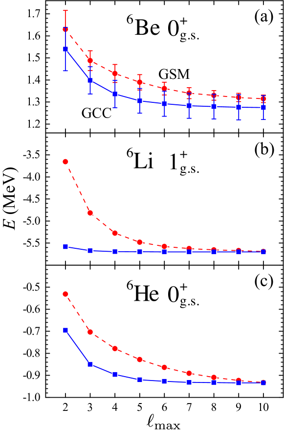
Figure 2: Comparison between GSM and GCC results for for the two-nucleon separation energies of ⁶Be, ⁶Li, and ⁶He obtained in different model spaces defined by $\ell_{\rm max}$. The bars in the panel (a) represent decay widths.

One can see in Fig.  2 that the calculations done with Jacobi coordinates converge faster than those with COSM coordinates. This comes from the attractive character of the nucleon-nucleon interaction, which results in the presence of a di-nucleon structure (see discussion below). Consequently, as T-type Jacobi coordinates well describe the di-nucleon cluster, they are able to capture correlations in a more efficient way than COSM coordinates. This is in agreement with the findings of Ref. Kruppa et al. (2014) based on the complex scaling method with COSM coordinates, who obtained the g.s. energy ⁶He that was slightly less bound as compared to results of Ref. Descouvemont et al. (2003) using Jacobi coordinates. In any case, our calculations have demonstrated that one obtains very similar results in GCC and GSM when sufficiently large model spaces are considered. As shown in Table 1, the energy difference between GCC and GSM predictions for $A=6$ systems is very small, around 20 keV for majority of states. The maximum deviation of $\sim$70 keV is obtained for the 3⁺ state of ⁶Li. However, because of the attractive character of the $T=0$ interaction, the GSM calculation for this state has not fully converged at $\ell_{\rm max}=10$.

Table 1: Comparison between energies (in MeV) and widths (in keV) predicted for ⁶He, ⁶Li, and ⁶Be in GSM and GCC in the $\ell_{\rm max}=10$ model space.

Nucleus	$J^{\pi}$	GSM	GCC
6He	$0^{+}$	$-0.933$	$-0.934$
	$2^{+}$	0.800(98)	0.817(42)
6Li	$1^{+}$	$-5.680$	$-5.698$
	$3^{+}$	$-2.097$	$-2.167$
	$0^{+}$	$-0.041$	$-0.048$
6Be	$0^{+}$	1.314(25)	1.275(54)

Motivated by the discussion in Ref. Descouvemont et al. (2003), we have also studied the effect of the $\ell$-dependent core-nucleus potential. To this end, we changed the WS strength $V_{0}$ from 47 MeV to 49 MeV for the $\ell=1$ partial waves while keeping the standard strength for the remaining $\ell$ values. As seen in Fig. 3, the convergence behavior obtained with Jacobi and COSM coordinates is fairly similar to that shown in Fig. 2, where the WS strength $V_{0}$ is the same for all partial waves. For $\ell_{\rm max}=12$, the difference between GSM and GCC energies of ⁶He becomes very small. This result is consistent with the findings of Ref. (Zhukov et al., 1993) that the recoil effect can indeed be successfully eliminated using COSM coordinates at the expense of reduced convergence.

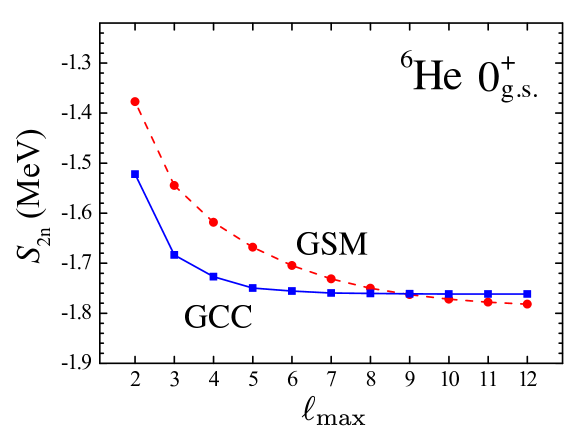
Figure 3: Similar as in Fig. 2 but for the two-neutron separation energy of ⁶He obtained with the angular-momentum dependent Hamiltonian, see text for details.

In order to see whether the difference between the model spaces of GCC and GSM can be compensated by renormalizing the effective Hamiltonian, we slightly readjusted the depth of the WS potential in GCC calculations to reproduce the g.s. GSM energy of ⁶He at model space $\ell_{\rm max}=7$. As a result, the strength $V_{0}$ changed from 47 MeV to 46.9 MeV. Except for the 2⁺ state of ⁶He, the GSM and GCC energies for $A=6$ systems got significantly closer as a result of such a renormalization. This indicates that the differences between Jacobi coordinates and COSM coordinates can be partly accounted for by refitting interaction parameters, even though model spaces and asymptotic behavior are different.

GCC is also in rough agreement with GSM when comparing decay widths, considering that they are very sensitive to the asymptotic behavior of the wave function, which is treated differently with Jacobi and COSM coordinates. Also, the presence of the recoil term in GSM, which is dealt with by means of the HO expansion, is expected to impact the GSM results for decay widths.

In order to check the precision of decay widths calculated with GCC, we adopted the current expression Humblet and Rosenfeld (1961):

$$\Gamma=i\frac{\int(\Psi^{\dagger}~{}\hat{\bf H}~{}\Psi-\Psi~{}\hat{\bf H}~{}\Psi^{\dagger})~{}d{\mbox{\boldmath$x$}}d{\mbox{\boldmath$y$}}}{\int|\Psi|^{2}d{\mbox{\boldmath$x$}}d{\mbox{\boldmath$y$}}},$$ (15)

which can be expressed in hyperspherical coordinates as Grigorenko et al. (2000); Grigorenko and Zhukov (2007):

$$\Gamma=i\frac{\hbar^{2}}{m}\frac{\left.\int d\Omega_{5}{\rm Im}[\psi\frac{\partial}{\partial\rho}\psi^{\dagger}]\right|_{\rho=\rho_{\rm max}}}{\int^{\rho_{\rm max}}_{0}|\psi|^{2}d\rho d\Omega_{5}},$$ (16)

where $\rho_{\rm max}$ is larger than the nuclear radius (in general, the decay width should not depend on the choice of $\rho_{\rm max}$). By using the current expression, we obtain $\Gamma$=42 keV for 2⁺ state of ⁶He and $\Gamma$=54 keV for 0⁺ state of ⁶Be, which are practically the same as the GCC values of Table 1 obtained from the direct diagonalization.

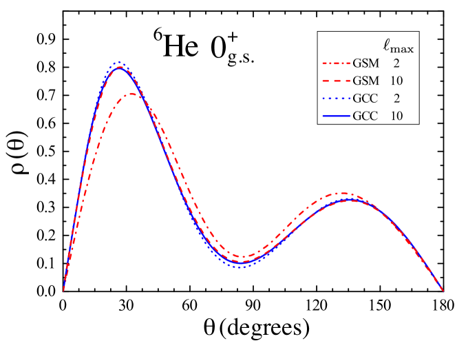
Figure 4: Comparison between GSM and GCC results for the two-neutron angular correlation in ⁶He for different model spaces defined by $\ell_{\rm max}$.

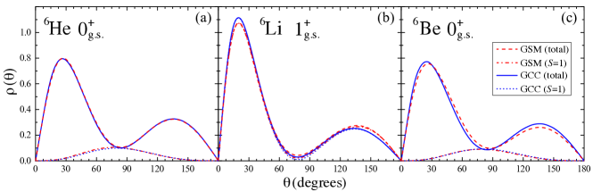
Figure 5: Two-nucleon angular densities (total and in the $S=1$ channel) in the g.s. configurations of ⁶He (a), ⁶Li (b), and ⁶Be (c) obtained in GSM and GCC with $\ell_{\rm max}=10$.

We now discuss the angular correlation of the two valence neutrons in the g.s. of ⁶He. Figure 4 shows GSM and GCC results for model spaces defined by different values of $\ell_{\rm max}$. The distribution $\rho(\theta)$ shows two maxima Zhukov et al. (1993); Hagino and Sagawa (2005); Horiuchi and Suzuki (2007); Kikuchi et al. (2010); Papadimitriou et al. (2011); Kruppa et al. (2014); Hagino and Sagawa (2016b). The higher peak, at a small opening angle, can be associated with a dineutron configuration. The second maximum, found in the region of large angles, represents the cigarlike configuration. The GCC results for $\ell_{\rm max}=2$ and 10 are already very close. This is not the case for the GSM, which shows sensitivity to the cutoff value of $\ell$. This is because the large continuum space, including states of positive and negative parity is needed in the COSM picture to describe dineutron correlations Catara et al. (1984); Pillet et al. (2007); Papadimitriou et al. (2011); Hagino and Sagawa (2014); Fossez et al. (2017). Indeed, as $\ell_{\rm max}$ increases, the angular correlations obtained in GSM and GCC are very similar. This indicates that Jacobi and COSM descriptions of $\rho(\theta)$ are essentially equivalent provided that the model space is sufficiently large.

In order to benchmark GCC and GSM calculations for the valence-proton case, in Fig. 5 we compare two-nucleon angular correlations for $A=6$ nuclei ⁶He, ⁶Li, and ⁶Be. Similar to Refs. Hagino and Sagawa (2005); Papadimitriou et al. (2011), we find that the $T=1$ configurations have a dominant $S=0$ component, in which the two neutrons in ⁶He or two protons in ⁶Be are in the spin singlet state. The amplitude of the $S=1$ density component is small. For all nuclei, GCC and GSM angular correlations are close.

Similar to ⁶He, the two peaks in ⁶Be indicate diproton and cigarlike configurations Oishi et al. (2014) (see also Refs. Garrido et al. (2007); Grigorenko et al. (2009b, 2012); Egorova et al. (2012); R. Álvarez-Rodríguez and Fedorov (2012)). It is to be noted that the dineutron peak in ⁶He is slightly higher than the diproton maximum in ⁶Be. This is due to the repulsive character of the Coulomb interaction between valence protons. The large maximum at small opening angles seen in ⁶Li corresponds to the deuteron-like structure. As discussed in Ref. Horiuchi and Suzuki (2007), this peak is larger that the the dineutron correlation in ⁶He. Indeed, the valence proton-neutron pair in ⁶Li is very strongly correlated because the $T=0$ interaction is much stronger than the $T=1$ interaction. The different features in the two-nucleon angular correlations in the three $A=6$ systems shown in Fig. 5 demonstrate that the angular correlations contain useful information on the effective interaction between valence nucleons.

III.2 Structure of unbound ²⁶O

After benchmarking GSM and GCC for $A=6$ systems, we apply both models to ²⁶O, which is believed to be a threshold dineutron structure Lunderberg et al. (2012); Kohley et al. (2013); Grigorenko and Zhukov (2015); Kondo et al. (2016); Hagino and Sagawa (2016a, b); Fossez et al. (2017).

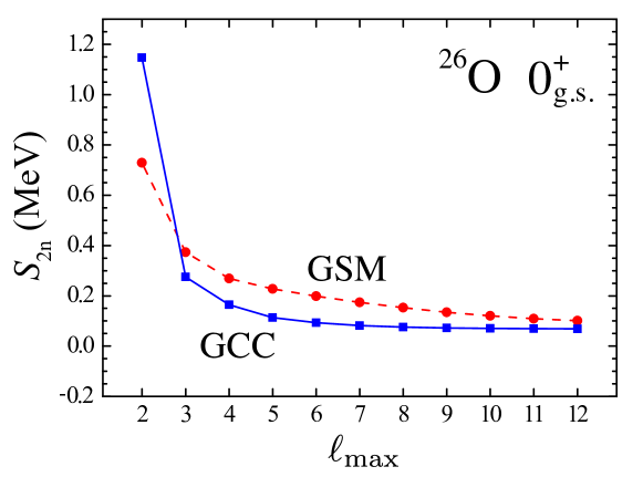
Figure 6: Two-neutron separation energy of the g.s. of ²⁶O computed with GSM and GCC for different values of $\ell_{\rm max}$.

It is a theoretical challenge to reproduce the resonances in ²⁶O as both continuum and high partial waves must be considered. As ²⁴O can be associated with the subshell closure in which the $0d_{5/2}$ and $1s_{1/2}$ neutron shells are occupied Tshoo et al. (2012), it can be used as core in our three-body model.

Figure 6 illustrates the convergence of the g.s. of ²⁶O with respect to $\ell_{\rm max}$ in GSM and GCC calculations. It is seen that in the GCC approach the energy converges nearly exponentially and that the stable result is practically reached at $\ell_{\rm max}=7$. While slightly higher in energy, the GSM results are quite satisfactory, as they differ only by about 30 keV from the GCC benchmark. Still, it is clear that $\ell_{\rm max}=12$ is not sufficient to reach the full convergence in GSM.

The calculated energies and widths of g.s. and 2⁺ state of ²⁶O are displayed in Table 2; they are both consistent with the most recent experimental values Kondo et al. (2016).

Table 2: Energies and widths (all in keV) predicted for ²⁶O in GSM and GCC in the $\ell_{\rm max}=12$ model space. Also shown are the dominant GSM ($\ell_{1}$, $\ell_{2}$) and GCC ($\ell_{x}$, $\ell_{y}$) configurations.

$J^{\pi}$	GSM		GCC
$0^{+}$	101	81% ($d,d$)	69	46% ($p,p$)
		11% ($f,f$)		44% ($s,s$)
		7% ($p,p$)		3% ($d,d$)
$2^{+}$	1137(33)	77% ($d,d$)	1150(14)	28% ($f,p$)
		7% ($p,p$)		27% ($p,f$)
		7% ($d,s$)		10% ($d,d$)

The amplitudes of dominant configurations listed in Table 2 illustrate the importance of considering partial waves of different parity in the GSM description of a dineutron g.s. configuration in ²⁶O Fossez et al. (2017).

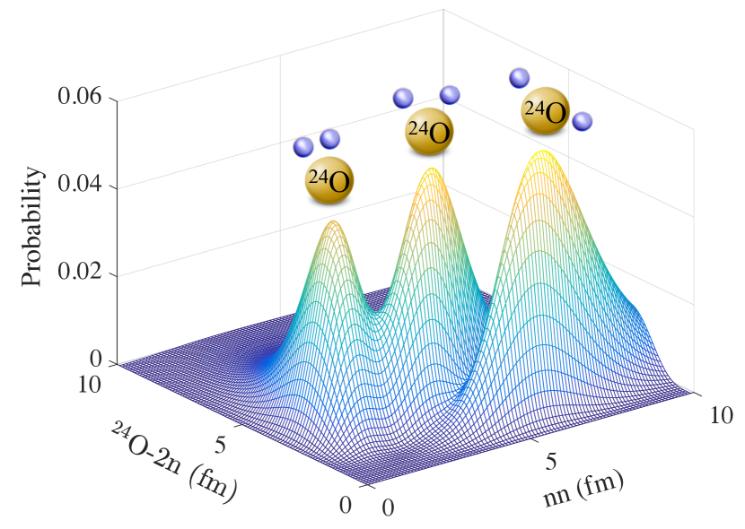
Figure 7: GCC wave function of the g.s. of ²⁶O in the Jacobi coordinates $nn$ and ²⁴O$-2n$.

The g.s. wave function of ²⁶O computed in GCC is shown in Fig. 7 in the Jacobi coordinates. The corresponding angular distribution is displayed in Fig. 8.

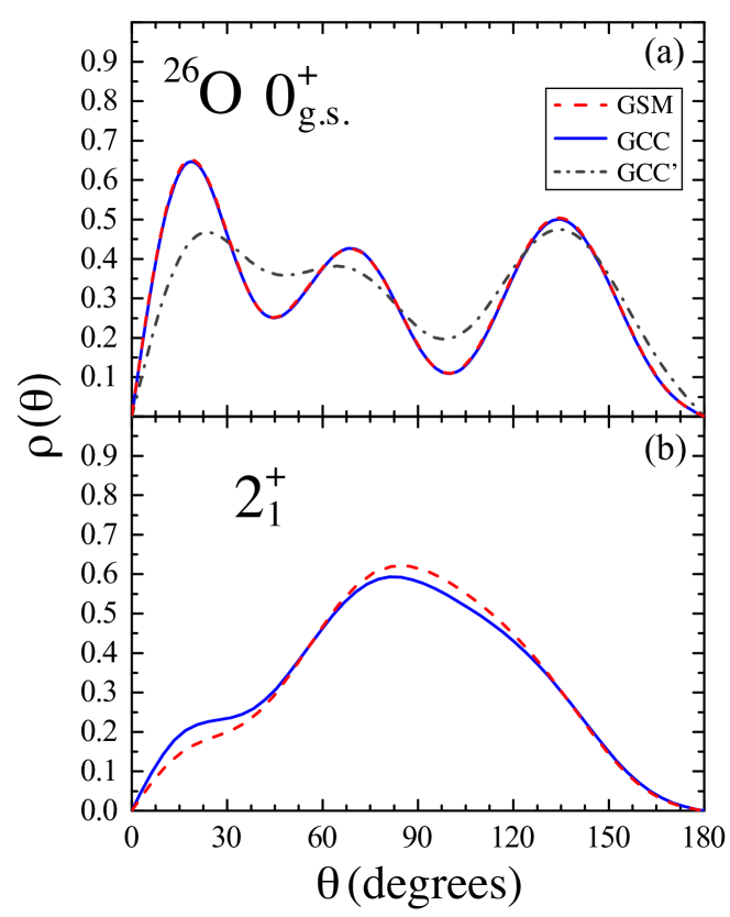
Figure 8: Two-neutron angular correlation for the 0⁺ g.s. (a) and 2${}^{+}_{1}$ state (b) configuration of ²⁶O computed with GCC (solid line) and GSM (dashed line) with $\ell_{\rm max}=10$. The dash-dotted curve labeled GCC’ in panel (a) shows GCC results obtained with the strength of the neutron-neutron interaction reduced by 50%.

Three pronounced peaks associated with the dineutron, triangular, and cigarlike configurations Hagino and Sagawa (2016a); Hove et al. (2017) can be identified. In GCC, the ($\ell_{x}$, $\ell_{y}$) = ($s,s$), ($p,p$) components dominate the g.s. wave function of ²⁶O; this is consistent with a sizable clusterization of the two neutrons. In COSM coordinates, it is the ($\ell_{1}$, $\ell_{2}$) = ($d,d$) configuration that dominates, but the the negative-parity ($f,f$) and ($p,p$) channels contribute with $\sim$20%. Again, it is encouraging to see that with $\ell_{\rm max}=10$ both approaches predict very similar two-nucleon densities.

In Table 2 we also display the predicted structure of the excited 2⁺ state of ²⁶O . The predicted energy is close to experiment Kondo et al. (2016) and other theoretical studies, see, e.g., Hagino and Sagawa (2016a); Grigorenko and Zhukov (2015); Volya and Zelevinsky (2006); Tsukiyama et al. (2015); Bogner et al. (2014). We obtain a small width for this state, which is consistent with the GSM+DMRG calculations of Ref. Fossez et al. (2017). The GCC occupations of Table 2 indicate that the wave function of the 2⁺ state is spread out in space, as the main three configurations, of cluster type, only contribute to the wave function with only 65%. When considering the GSM wave function, the ($d,d$) configuration dominates. The corresponding two-neutron angular correlation shown in Fig. 8(b) exhibits a broad distribution with a maximum around 90^∘. This situation is fairly similar to what has been predicted for the 2⁺ state of ⁶He Papadimitriou et al. (2011); Kruppa et al. (2014).

Finally, it is interesting to study how the neutron-neutron interaction impacts the angular correlation. To this end, Fig. 8(a) shows $\rho(\theta)$ obtained with the Minnesota neutron-neutron interaction whose strength has been reduced by 50%. While there are still three peaks present, the distribution becomes more uniform and the dineutron component no longer dominates. We can this conclude that the $nn$ angular correlation can be used as an indicator of the interaction between valence nucleons.

IV Conclusions

We developed a Gamow coupled-channel approach in Jacobi coordinates with the Berggren basis to describe structure and decays of three-body systems. We benchmarked the performance of the new approach against the Gamow Shell Model. Both methods are capable of considering large continuum spaces but differ in their treatment of three-body asymptotics, center-of-mass motion, and Pauli operator. In spite of these differences, we demonstrated that the Jacobi-coordinate-based framework (GCC) and COSM-based framework (GSM) can produce fairly similar results, provided that the continuum space is sufficiently large.

For benchmarking and illustrative examples we choose ⁶He, ⁶Li, and ⁶Be, and ²⁶O – all viewed as a core-plus-two-nucleon systems. We discussed the spectra, decay widths, and nucleon-nucleon angular correlations in these nuclei. The Jacobi coordinates capture cluster correlations (such as dineutron and deuteron-type) more efficiently; hence, the convergence rate of GCC is faster than that of GSM.

For ²⁶O, we demonstrated the sensitivity of $nn$ angular correlation to the valence-neutron interaction. It will be interesting to investigate this aspect further to provide guidance for future experimental investigations of di-nucleon correlations in bound and unbound states of dripline nuclei.

In summary, we developed an efficient approach to structure and decays of three-cluster systems. The GCC method is based on a Hamiltonian involving a two-body interaction between valence nucleons and a one-body field representing the core-nucleon potential. The advantage of the model is its ability to correctly describe the three-body asymptotic behavior and the efficient treatment of the continuum space, which is of particular importance for the treatment of threshold states and narrow resonances. The model can be easily extended along the lines of the resonating group method by introducing a microscopic picture of the core Navrátil et al. (2016); Jaganathen et al. (2014). Meanwhile, it can be used to elucidate experimental findings on dripline systems, and to provide finetuned predictions to guide $A$-body approaches.