An Open Source C++ Implementation of Multi-Threaded Gaussian Mixture Models, k-Means and Expectation Maximisation

Conrad Sanderson ^†⋄∗ and Ryan Curtin ^‡∗

^† Data61, CSIRO, Australia
^‡ Symantec Corporation, USA
^⋄ University of Queensland, Australia
^∗ Arroyo Consortium

Abstract

Modelling of multivariate densities is a core component in many signal processing, pattern recognition and machine learning applications. The modelling is often done via Gaussian mixture models (GMMs), which use computationally expensive and potentially unstable training algorithms. We provide an overview of a fast and robust implementation of GMMs in the C++ language, employing multi-threaded versions of the Expectation Maximisation (EM) and k-means training algorithms. Multi-threading is achieved through reformulation of the EM and k-means algorithms into a MapReduce-like framework. Furthermore, the implementation uses several techniques to improve numerical stability and modelling accuracy. We demonstrate that the multi-threaded implementation achieves a speedup of an order of magnitude on a recent 16 core machine, and that it can achieve higher modelling accuracy than a previously well-established publically accessible implementation. The multi-threaded implementation is included as a user-friendly class in recent releases of the open source Armadillo C++ linear algebra library. The library is provided under the permissive Apache 2.0 license, allowing unencumbered use in commercial products.

Introduction

Modelling multivariate data through a convex mixture of Gaussians, also known as a Gaussian mixture model (GMM), has many uses in fields such as signal processing, econometrics, pattern recognition, machine learning and computer vision. Examples of applications include multi-stage feature extraction for action recognition [4], modelling of intermediate features derived from deep convolutional neural networks [11, 12, 16], classification of human epithelial cell images [32], implicit sparse coding for face recognition [33], speech-based identity verification [28], and probabilistic foreground estimation for surveillance systems [26]. GMMs are also commonly used as the emission distribution for hidden Markov models [2].

In the GMM approach, a distribution of samples (vectors) is modelled as:

$$p({\boldsymbol{x}}|\lambda)=\sum\nolimits_{g=1}^{N_{G}}w_{g}\leavevmode\nobreak\ {{\mathcal{N}}}({\boldsymbol{x}}|{\boldsymbol{\mu}}_{g},{\boldsymbol{\Sigma}}_{g})$$ (1)

where ${\boldsymbol{x}}$ is a $D$-dimensional vector, $w_{g}$ is the weight for component $g$ (with constraints $\sum\nolimits_{g=1}^{N_{G}}w_{g}=1$, $w_{g}\geq 0$), and ${{\mathcal{N}}}({\boldsymbol{x}}|{\boldsymbol{\mu}},{\boldsymbol{\Sigma}})$ is a $D$-dimensional Gaussian density function with mean ${\boldsymbol{\mu}}$ and covariance matrix ${\boldsymbol{\Sigma}}$:

$${{\mathcal{N}}}({\boldsymbol{x}}|{\boldsymbol{\mu}},{\boldsymbol{\Sigma}})=\frac{1}{(2\pi)^{\frac{D}{2}}|{\boldsymbol{\Sigma}}|^{\frac{1}{2}}}\exp\left[-\frac{1}{2}({\boldsymbol{x}}-{\boldsymbol{\mu}})^{\top}{\boldsymbol{\Sigma}}^{-1}({\boldsymbol{x}}-{\boldsymbol{\mu}})\right]$$ (2)

where $|{\boldsymbol{\Sigma}}|$ and ${\boldsymbol{\Sigma}}^{-1}$ denote the determinant and inverse of ${\boldsymbol{\Sigma}}$, respectively, while ${\boldsymbol{x}}^{\top}$ denotes the transpose of ${\boldsymbol{x}}$. The full parameter set can be compactly stated as $\lambda=\{w_{g},{\boldsymbol{\mu}}_{g},{\boldsymbol{\Sigma}}_{g}\}_{g=1}^{N_{G}}$, where $N_{G}$ is the number of Gaussians.

Given a training dataset and a value for $N_{G}$, the estimation of $\lambda$ is typically done through a tailored instance of Expectation Maximisation (EM) algorithm [8, 21, 24, 27]. The k-means algorithm [3, 9, 18] is also typically used for providing the initial estimate of $\lambda$ for the EM algorithm. Choosing the optimal $N_{G}$ is data dependent and beyond the scope of this work; see [14, 25] for example methods.

Unfortunately, GMM parameter estimation via the EM algorithm is computationally intensive and can suffer from numerical stability issues. Given the ever growing sizes of datasets and the need for fast, robust and accurate modelling of such datasets, we have provided an open source implementation of multi-threaded (parallelised) versions of the k-means and EM algorithms. In addition, core functions are recast in order to considerably reduce the likelihood of numerical instability due to floating point underflows and overflows. The implementation is provided as a user-friendly class in recent releases of the cross-platform Armadillo C++ linear algebra library [29, 30]. The library is licensed under the permissive Apache 2.0 license [31], thereby allowing unencumbered use in commercial products.

We continue the paper as follows. In Section 2 we provide an overview of parameter estimation via the EM algorithm, its reformulation for multi-threaded execution, and approaches for improving numerical stability. In Section 3 we provide a summary of the k-means algorithm along with approaches for improving its convergence and modelling accuracy. The implementation in C++ is overviewed in Section 4, where we list and describe the user accessible functions. In Section 5 we provide a demonstration that the implementation can achieve a speedup of an order of magnitude on a recent 16 core machine, as well as obtain higher modelling accuracy than a previously well-established publically accessible implementation.

Expectation Maximisation and Multi-Threading

The overall likelihood for a set of samples, $X=\{{\boldsymbol{x}}_{i}\}_{i=1}^{N_{V}}$, is found using $p(X|\lambda)=\prod\nolimits_{i=1}^{N_{V}}p({\boldsymbol{x}}_{i}|\lambda)$. A parameter set $\lambda$ that suitably models the underlying distribution of $X$ can be estimated using a particular instance of the Expectation Maximisation (EM) algorithm [8, 21, 24, 27]. As its name suggests, the EM algorithm is comprised of iterating two steps: the expectation step, followed by the maximisation step. GMM parameters generated by the previous iteration ($\lambda^{\textrm{old}}$) are used by the current iteration to generate a new set of parameters ($\lambda^{\textrm{new}}$), such that $p(X|\lambda^{\textrm{new}})\geq p(X|\lambda^{\textrm{old}})$.

In a direct implementation of the EM algorithm specific to GMMs, the estimated versions of the parameters ($\widehat{w}_{g}$, $\widehat{{\boldsymbol{\mu}}}_{g}$, $\widehat{{\boldsymbol{\Sigma}}}_{g}$) within one iteration are calculated as follows:

$$l_{g,i} = \frac{w_{g}\leavevmode\nobreak\ {{\mathcal{N}}}({\boldsymbol{x}}_{i}|{\boldsymbol{\mu}}_{g},{\boldsymbol{\Sigma}}_{g})}{\sum\nolimits_{k=1}^{N_{G}}w_{k}\leavevmode\nobreak\ {{\mathcal{N}}}({\boldsymbol{x}}_{i}|{\boldsymbol{\mu}}_{k},{\boldsymbol{\Sigma}}_{k})},$$ (3)

$$L_{g} = \sum\nolimits_{i=1}^{N_{V}}l_{g,i},$$ (4)

$$\widehat{w}_{g} = \frac{L_{g}}{N_{V}},$$ (5)

$$\widehat{{\boldsymbol{\mu}}}_{g} = \frac{1}{L_{g}}\sum\nolimits_{i=1}^{N_{V}}{\boldsymbol{x}}_{i}\leavevmode\nobreak\ l_{g,i},$$ (6)

$$\widehat{{\boldsymbol{\Sigma}}}_{g} = \frac{1}{L_{g}}\sum\nolimits_{i=1}^{N_{V}}({\boldsymbol{x}}_{i}-\widehat{{\boldsymbol{\mu}}}_{g})({\boldsymbol{x}}_{i}-\widehat{{\boldsymbol{\mu}}}_{g})^{\top}l_{g,i}.$$ (7)

Once the estimated parameters for all Gaussians are found, the parameters are updated, $\left\{w_{g},{\boldsymbol{\mu}}_{g},{\boldsymbol{\Sigma}}_{g}\right\}_{g=1}^{N_{G}}=\left\{\widehat{w}_{g},\widehat{{\boldsymbol{\mu}}}_{g},\widehat{{\boldsymbol{\Sigma}}}_{g}\right\}_{g=1}^{N_{G}}$, and the iteration starts anew. The process is typically repeated until the number of iterations has reached a pre-defined number, and/or the increase in the overall likelihood after each iteration falls below a pre-defined threshold.

In Eqn. (3), $l_{g,i}\in[0,1]$ is the a-posteriori probability of Gaussian $g$ given ${\boldsymbol{x}}_{i}$ and current parameters. Thus the estimates $\widehat{{\boldsymbol{\mu}}}_{g}$ and $\widehat{{\boldsymbol{\Sigma}}}_{g}$ are weighted versions of the sample mean and sample covariance, respectively.

Overall, the algorithm is a hill climbing procedure for maximising $p(X|\lambda)$. While there are no guarantees that it will reach a global maximum, it is guaranteed to monotonically converge to a saddle point or a local maximum [8, 9, 22]. The above implementation can also be interpreted as an unsupervised probabilistic clustering procedure, with $N_{G}$ being the assumed number of clusters. For a full derivation of the EM algorithm tailored to GMMs, the reader is directed to [2, 27] or Appendix A.

Reformulation for Multi-Threaded Execution

The EM algorithm is quite computationally intensive. This is in large part due to the use of the $\exp(\cdot)$ function, which needs to be applied numerous times for each and every sample. Fortunately, CPUs with a multitude of cores are now quite common and accessible, allowing for multi-threaded (parallel) execution.

One approach for parallelisation is the MapReduce framework [7], where data is split into chunks and farmed out to separate workers for processing (mapping). The results are then collected and combined (reduced) to produce the final result. Below we provide a reformulation of the EM algorithm into a MapReduce-like framework.

As Eqn. (3) can be executed independently for each sample, the summations in Eqns. (4) and (6) can be split into separate sets of summations, where the summation in each set can be executed independently and in parallel with other sets. To allow similar splitting of the summation for calculating covariance matrices, Eqn. (7) needs to be rewritten into the following form:

$$\widehat{{\boldsymbol{\Sigma}}}_{g}=\frac{1}{L_{g}}\left[\sum\nolimits_{i=1}^{N_{V}}{\boldsymbol{x}}_{i}{\boldsymbol{x}}_{i}^{\top}l_{g,i}\right]-\widehat{{\boldsymbol{\mu}}}_{g}\widehat{{\boldsymbol{\mu}}}_{g}^{\top}.$$ (8)

The multi-threaded estimation of the parameters can now be formally stated as follows. Given $N_{T}$ threads, the training samples are split into $N_{T}$ chunks, with each chunk containing approximately the same amount of samples. For thread with index $t\in[1,N_{T}]$, the start index of the samples is denoted by $i^{[t]}_{\textrm{start}}$, while the end index is denoted by $i^{[t]}_{\textrm{end}}$. For each thread $t$ and Gaussian $g\in[1,N_{G}]$, accumulators $\widetilde{L}_{g}^{[t]}$, $\widetilde{{\boldsymbol{\mu}}}_{g}^{[t]}$ and $\widetilde{{\boldsymbol{\Sigma}}}_{g}^{[t]}$ are calculated as follows:

$$\widetilde{L}_{g}^{[t]} = \sum\nolimits_{j=i^{[t]}_{\textrm{start}}}^{i^{[t]}_{\textrm{end}}}l_{g,j},$$ (9)

$$\widetilde{{\boldsymbol{\mu}}}_{g}^{[t]} = \sum\nolimits_{j=i^{[t]}_{\textrm{start}}}^{i^{[t]}_{\textrm{end}}}l_{g,j}\leavevmode\nobreak\ {\boldsymbol{x}}_{j},$$ (10)

$$\widetilde{{\boldsymbol{\Sigma}}}_{g}^{[t]} = \sum\nolimits_{j=i^{[t]}_{\textrm{start}}}^{i^{[t]}_{\textrm{end}}}l_{g,j}\leavevmode\nobreak\ {\boldsymbol{x}}_{j}{\boldsymbol{x}}_{j}^{\top}.$$ (11)

where $l_{g,j}$ is defined in Eqn. (3).

Once the accumulators for all threads are calculated, for each Gaussian $g$ the reduction operation combines them to form the estimates of $\widehat{{\boldsymbol{\mu}}}_{g}$ and $\widehat{{\boldsymbol{\Sigma}}}_{g}$ as follows:

$$L_{g} = \sum\nolimits_{t=1}^{N_{T}}\widetilde{L}_{g}^{[t]},$$ (12)

$$\widehat{{\boldsymbol{\mu}}}_{g} = \frac{1}{L_{g}}\sum\nolimits_{t=1}^{N_{T}}\widetilde{{\boldsymbol{\mu}}}_{g}^{[t]},$$ (13)

$$\widehat{{\boldsymbol{\Sigma}}}_{g} = \frac{1}{L_{g}}\sum\nolimits_{t=1}^{N_{T}}\widetilde{{\boldsymbol{\Sigma}}}_{g}^{[t]}-\widehat{{\boldsymbol{\mu}}}_{g}\widehat{{\boldsymbol{\mu}}}_{g}^{\top}.$$ (14)

The estimation of $\widehat{w}_{g}$ is as per Eqn. (5), but using $L_{g}$ from Eqn. (12).

Improving Numerical Stability

Due to the necessarily limited precision of numerical floating point representations [13, 23], the direct computation of Eqns. (1) and (2) can quickly lead to numerical underflows or overflows, which in turn lead to either poor models or a complete failure to estimate the parameters. To address this problem, the following reformulation can be used. First, logarithm version of Eqn. (2) is taken:

$$\log{{\mathcal{N}}}({\boldsymbol{x}}|{\boldsymbol{\mu}},{\boldsymbol{\Sigma}})=-\left\{\frac{D}{2}\log\left(2\pi\right)+\frac{1}{2}\leavevmode\nobreak\ \log(|{\boldsymbol{\Sigma}}|)\right\}-\frac{1}{2}({\boldsymbol{x}}-{\boldsymbol{\mu}})^{\top}{\boldsymbol{\Sigma}}^{-1}({\boldsymbol{x}}-{\boldsymbol{\mu}}),$$ (15)

which leads to the corresponding logarithm version of Eqn. (1):

$$\log\sum\nolimits_{g=1}^{N_{G}}w_{g}\leavevmode\nobreak\ {{\mathcal{N}}}({\boldsymbol{x}}\leavevmode\nobreak\ |\leavevmode\nobreak\ {\boldsymbol{\mu}}_{g},{\boldsymbol{\Sigma}}_{g})=\log\sum\nolimits_{g=1}^{N_{G}}\exp\left[\log\left\{w_{g}{{\mathcal{N}}}({\boldsymbol{x}}\leavevmode\nobreak\ |\leavevmode\nobreak\ {\boldsymbol{\mu}}_{g},{\boldsymbol{\Sigma}}_{g})\right\}\right].$$ (16)

The right hand side of Eqn. (16) can be expressed as a repeated addition in the form of:

$$\log\left(\exp\left[\log(a)\right]+\exp\left[\log(b)\right]\right),$$ (17)

which in turn can be rewritten in the form of:

$$\log(a)+\log\left(1+\exp\left[\log(b)-\log(a)\right]\right).$$ (18)

In the latter form, if we ensure that $\log(a)\geq\log(b)$ (through swapping $\log(a)$ and $\log(b)$ when required), the exponential will always produce values $\leq 1$ which helps to reduce the occurrence of overflows. Overall, by keeping most of the computation in the log domain, both underflows and overflows are considerably reduced.

A further practical issue is the occurrence of degenerate or ill-conditioned covariance matrices, stemming from either not enough samples with $l_{g,i}>0$ contributing to the calculation of $\widehat{{\boldsymbol{\Sigma}}}_{g}$ in Eqn. (7), or from too many samples which are essentially the same (ie., very low variance). When the diagonal entries in a covariance matrix are too close to zero, inversion of the matrix is unstable and can cause the calculated log-likelihood to become unreliable or non-finite. A straightforward and effective approach to address this problem is to place an artificial floor on the diagonal entries in each covariance matrix after each EM iteration. While the optimum value of the floor is data dependent, a small positive constant is typically sufficient to promote numerical stability and convergence.

Initialisation via Multi-Threaded k-Means

As a starting point, the initial means can be set to randomly selected training vectors, the initial covariance matrices can be set equal to identity matrices, and the initial weights can be uniform. However, the $\exp(\cdot)$ function as well as the matrix inverse in Eqn. (2) are typically quite time consuming to compute. In order to speed up training, the initial estimate of $\lambda$ is typically provided via the k-means clustering algorithm [3, 9, 15] which avoids such time consuming operations.

The baseline k-means clustering algorithm is a straightforward iterative procedure comprised of two steps: (i) calculating the distance from each sample to each mean, and (ii) calculating the new version of each mean as the average of samples which were found to be the closest to the previous version of the corresponding mean. The required number of iterations is data dependent, but about 10 iterations are often sufficient to generate a good initial estimate of $\lambda$.

The $k$-means algorithm can be interpreted as a simplified version (or special case) of the EM algorithm for GMMs [15]. Instead of each sample being assigned a set probabilities representing cluster membership (soft assignment), each sample is assigned to only one cluster (hard assignment). Furthermore, it can be assumed that the covariance matrix of each Gaussian is non-informative, diagonal, and/or shared across all Gaussians. More formally, the estimation of model parameters is as per Eqns. (5), (6) and (7), but $l_{g,i}$ is redefined as:

$$l_{g,i}=\left\{\begin{array}[]{ll}1,&\mbox{if}\leavevmode\nobreak\ g=\operatorname*{argmin}\limits_{k=1,\cdots,N_{G}}\operatorname{dist}({\boldsymbol{\mu}}_{k},{\boldsymbol{x}}_{i})\\ 0,&\mbox{otherwise}.\end{array}\right.$$ (19)

where $\operatorname{dist}({\boldsymbol{a}},{\boldsymbol{b}})$ is a distance metric. Apart from this difference, the parameter estimation is the same as for EM. As such, multi-threading is achieved as per Section 2.1.

We note that it is possible to implement the k-means algorithm is a multitude of ways, such as the cluster splitting LBG algorithm [18], or use an elaborate strategy for selecting the initial means [1]. While there are also alternative and more complex implementations offering relatively fast execution [10], we have elected to adapt the baseline k-means algorithm due to its straightforward amenability to multi-threading.

Issues with Modelling Accuracy and Convergence

A typical and naive choice for the distance in Eqn. (19) is the squared Euclidean distance, $\operatorname{dist}({\boldsymbol{a}},{\boldsymbol{b}})=\|{\boldsymbol{a}}-{\boldsymbol{b}}\|^{2}_{2}$. However, for multivariate datasets formed by combining data from various sensors, there is a notable downside to using the Euclidean distance. When one of the dimensions within the data has a much larger range than the other dimensions, it will dominate the contribution to the overall distance, with the other dimensions effectively ignored. This can adversely skew the initial parameter estimates, easily leading to poor initial conditions for the EM algorithm. This in turn can lead to poor modelling, as the EM algorithm is only guaranteed to reach a local maximum [8, 9, 22]. To address this problem, the squared Mahalanobis distance can be used [3, 9]:

$$\operatorname{dist}({\boldsymbol{a}},{\boldsymbol{b}})=({\boldsymbol{a}}-{\boldsymbol{b}})^{\top}{\boldsymbol{\Sigma}}^{-1}_{\mathrm{global}}({\boldsymbol{a}}-{\boldsymbol{b}}),$$ (20)

where ${\boldsymbol{\Sigma}}_{\mathrm{global}}$ is a global covariance matrix, estimated from all available training data. To maintain efficiency, ${\boldsymbol{\Sigma}}_{\mathrm{global}}$ is typically diagonal, which makes calculating its inverse straightforward (ie., reciprocals of the values on the main diagonal).

In practice it is possible that while iterating at least one of the means has no vectors assigned to it, becoming a “dead” mean. This might stem from an unfortunate starting point, or specifying a relatively large value for $N_{G}$ for modelling a relatively small dataset. As such, an additional heuristic is required to attempt to resolve this situation. An effective approach for resurrecting a “dead” mean is to make it equal to one of the vectors that has been assigned to the most “popular” mean, where the most “popular” mean is the mean that currently has the most vectors assigned to it.

Implementation in C++

We have provided a numerical implementation of Gaussian Mixture Models in the C++ language as part of recent releases of the open source Armadillo C++ linear algebra library [29]. The library is available under the permissive Apache 2.0 license [31], and can be obtained from http://arma.sourceforge.net. To considerably reduce execution time, the implementation contains multi-threaded versions of the EM and k-means training algorithms (as overviewed in Sections 2 and 3). Implementation of multi-threading is achieved with the aid of OpenMP pragma directives [5].

There are two main choices for the type of covariance matrix ${\boldsymbol{\Sigma}}$: full and diagonal. While full covariance matrices have more capacity for modelling data, diagonal covariance matrices provide several practical advantages:

1. the computationally expensive (and potentially unstable) matrix inverse operation in Eqn. (2) is reduced to simply to taking the reciprocals of the diagonal elements,

2. the determinant operation is considerably simplified to taking the product of the diagonal elements,

3. diagonal covariance matrices contain fewer parameters that need to be estimated, and hence require fewer training samples [9].

Given the above practical considerations, the implementation uses diagonal covariance matrices. We note that diagonal covariance GMMs with $N_{G}>1$ can model distributions of samples with correlated elements, which in turn suggests that full covariance GMMs can be approximated using diagonal covariance GMMs with a larger number of Gaussians [28].

User Accessible Classes and Functions

The implementation is provided as two user-friendly classes within the arma namespace: gmm_diag and fgmm_diag. The former uses double precision floating point values, while the latter uses single precision floating point values. For an instance of the double precision gmm_diag class named as M, its member functions and variables are listed below. The interface allows the user full control over the parameters for GMM fitting, as well as easy and flexible access to the trained model. Figure 1 contains a complete C++ program which demonstrates usage of the gmm_diag class.

In the description below, all vectors and matrices refer to corresponding objects from the Armadillo library; scalars have the type double, matrices have the type mat, column vectors have the type vec, row vectors have the type rowvec, row vectors of unsigned integers have the type urowvec, and indices have the type uword (representing an unsigned integer). When using the single precision fgmm_diag class, all vector and matrix types have the f prefix (for example, fmat), while scalars have the type float. The word “heft” is explicitly used in the classes as a shorter version of “weight”, while keeping the same meaning with the context of GMMs.

1. M.log_p(V)
   return a scalar (double precision floating point value) representing the log-likelihood of column vector V

2. M.log_p(V, g)
   return a scalar (double precision floating point value) representing the log-likelihood of column vector V, according to Gaussian with index g (specified as an unsigned integer of type uword)

3. M.log_p(X)
   return a row vector (of type rowvec) containing log-likelihoods of each column vector in matrix X

4. M.log_p(X, g)
   return a row vector (of type rowvec) containing log-likelihoods of each column vector in matrix X, according to Gaussian with index g (specified as an unsigned integer of type uword)

5. M.avg_log_p(X)
   return a scalar (double precision floating point value) representing the average log-likelihood of all column vectors in matrix X

6. M.avg_log_p(X, g)
   return a scalar (double precision floating point value) representing the average log-likelihood of all column vectors in matrix X, according to Gaussian with index g (specified as an unsigned integer of type uword)

7. M.assign(V, dist_mode)
   return an unsigned integer (of type uword) representing the index of the closest mean (or Gaussian) to vector V; the parameter dist_mode is one of:

   1. Euclidean distance (takes only means into account)

   1. probabilistic “distance”, defined as the inverse likelihood (takes into account means, covariances and hefts)

8. M.assign(X, dist_mode)
   return a row vector of unsigned integers (of type urowvec) containing the indices of the closest means (or Gaussians) to each column vector in matrix X; parameter dist_mode is eucl_dist or prob_dist, as per the .assign() function above

9. M.raw_hist(X, dist_mode)
   return a row vector of unsigned integers (of type urowvec) representing the raw histogram of counts; each entry is the number of counts corresponding to a Gaussian; each count is the number times the corresponding Gaussian was the closest to each column vector in matrix X; parameter dist_mode is eucl_dist or prob_dist, as per the .assign() function above

10. M.norm_hist(X, dist_mode)
    similar to the .raw_hist() function above; return a row vector (of type rowvec) containing normalised counts; the vector sums to one; parameter dist_mode is either eucl_dist or prob_dist, as per the .assign() function above

11. M.generate()
    return a column vector (of type vec) representing a random sample generated according to the model’s parameters

12. M.generate(N)
    return a matrix (of type mat) containing N column vectors, with each vector representing a random sample generated according to the model’s parameters

13. M.n_gaus()
    return an unsigned integer (of type uword) containing the number of means/Gaussians in the model

14. M.n_dims()
    return an unsigned integer (of type uword) containing the dimensionality of the means/Gaussians in the model

15. M.reset(n_dims, n_gaus)
    set the model to have dimensionality n_dims, with n_gaus number of Gaussians, specified as unsigned integers of type uword; all the means are set to zero, all diagonal covariances are set to one, and all the hefts (weights) are set to be uniform

16. M.save(filename)
    save the model to a file and return a bool indicating either success (true) or failure (false)

17. M.load(filename)
    load the model from a file and return a bool indicating either success (true) or failure (false)

18. M.means
    read-only matrix (of type mat) containing the means (centroids), stored as column vectors

19. M.dcovs
    read-only matrix (of type mat) containing the diagonal covariances, with the set of diagonal covariances for each Gaussian stored as a column vector

20. M.hefts
    read-only row vector (of type rowvec) containing the hefts (weights)

21. M.set_means(X)
    set the means (centroids) to be as specified in matrix X (of type mat), with each mean (centroid) stored as a column vector; the number of means and their dimensionality must match the existing model

22. M.set_dcovs(X)
    set the diagonal covariances to be as specified in matrix X (of type mat), with the set of diagonal covariances for each Gaussian stored as a column vector; the number of diagonal covariance vectors and their dimensionality must match the existing model

23. M.set_hefts(V)
    set the hefts (weights) of the model to be as specified in row vector V (of type rowvec); the number of hefts must match the existing model

24. M.set_params(means, dcovs, hefts)
    set all the parameters at the same time, using matrices denoted as means and dcovs as well as the row vector denoted as hefts; the layout of the matrices and vectors is as per the .set_means(), .set_dcovs() and .set_hefts() functions above; the number of Gaussians and dimensionality can be different from the existing model

25. M.learn(data, n_gaus, dist_mode, seed_mode, km_iter, em_iter, var_floor, print_mode)
    learn the model parameters via the k-means and/or EM algorithms, and return a boolean value, with true indicating success, and false indicating failure; the parameters have the following meanings:

    1. data
       matrix (of type mat) containing training samples; each sample is stored as a column vector

    2. n_gaus
       set the number of Gaussians to n_gaus; to help convergence, it is recommended that the given data matrix (above) contains at least 10 samples for each Gaussian

    3. dist_mode
       specifies the distance used during the seeding of initial means and k-means clustering:

       1. Euclidean distance

       1. Mahalanobis distance, which uses a global diagonal covariance matrix estimated from the given training samples

    4. seed_mode
       specifies how the initial means are seeded prior to running k-means and/or EM algorithms:

       keep_existing	keep the existing model (do not modify the means, covariances and hefts)
       static_subset	a subset of the training samples (repeatable)
       random_subset	a subset of the training samples (random)
       static_spread	a maximally spread subset of training samples (repeatable)
       random_spread	a maximally spread subset of training samples (random start)

       Note that seeding the initial means with static_spread and random_spread can be more time consuming than with static_subset and random_subset; these seed modes are inspired by the so-called k-means++ approach [1], with the aim to improve clustering quality.

    5. km_iter
       the maximum number of iterations of the k-means algorithm; this is data dependent, but typically 10 iterations are sufficient

    6. em_iter
       the maximum number of iterations of the EM algorithm; this is data dependent, but typically 5 to 10 iterations are sufficient

    7. var_floor
       the variance floor (smallest allowed value) for the diagonal covariances; setting this to a small non-zero value can help with convergence and/or better quality parameter estimates

    8. print_mode
       boolean value (either true or false) which enables/disables the printing of progress during the k-means and EM algorithms

 

#include <armadillo> using namespace arma; int main()   {   // create synthetic data containing   // 2 clusters with normal distribution   uword d = 5;       // dimensionality   uword N = 10000;   // number of samples (vectors)   mat data(d, N, fill::zeros);   vec mean1 = linspace<vec>(1,d,d);   vec mean2 = mean1 + 2;   uword i = 0;   while(i < N)     {     if(i < N)  { data.col(i) = mean1 + randn<vec>(d); ++i; }     if(i < N)  { data.col(i) = mean1 + randn<vec>(d); ++i; }     if(i < N)  { data.col(i) = mean2 + randn<vec>(d); ++i; }     }   // model the data as a diagonal GMM with 2 Gaussians   gmm_diag model;   bool status = model.learn(data, 2, maha_dist, random_subset,                             10, 5, 1e-10, true);   if(status == false)  { cout << "learning failed" << endl; }   model.means.print("means:");   double overall_likelihood = model.avg_log_p(data);   rowvec     set_likelihood = model.log_p( data.cols(0,9) );   double  scalar_likelihood = model.log_p( data.col(0)    );   uword   gaus_id  = model.assign( data.col(0),    eucl_dist );   urowvec gaus_ids = model.assign( data.cols(0,9), prob_dist );   urowvec histogram1 = model.raw_hist (data, prob_dist);    rowvec histogram2 = model.norm_hist(data, eucl_dist);   model.save("my_model.gmm");   mat modified_dcovs = 2 * model.dcovs;   model.set_dcovs(modified_dcovs);   return 0;   }

 

Figure 1: An example C++ program which demonstrates usage of a subset of functions available in the gmm_diag class.

Evaluation

Speedup from Multi-Threading

To demonstrate the achievable speedup with the multi-threaded versions of the EM and k-means algorithms, we trained a GMM with 100 Gaussians on a recent 16 core machine using a synthetic dataset comprising 1,000,000 samples with 100 dimensions. 10 iterations of the k-means algorithm and 10 iterations of the EM algorithm were used. The samples were stored in double precision floating point format, resulting in a total data size of approximately 762 Mb.

Figure 2 shows that a speedup of an order of magnitude is achieved when all 16 cores are used. Specifically, for the synthetic dataset used in this demonstration, the training time was reduced from approximately 272 seconds to about 27 seconds. In each case, the k-means algorithm took approximately 30% of the total training time.

We note that the overall speedup is below the idealised linear speedup. This is likely due to overheads related to OpenMP and reduction operations described in Section 2.1, as well as memory access contention, stemming from concurrent access to memory by multiple cores [20].

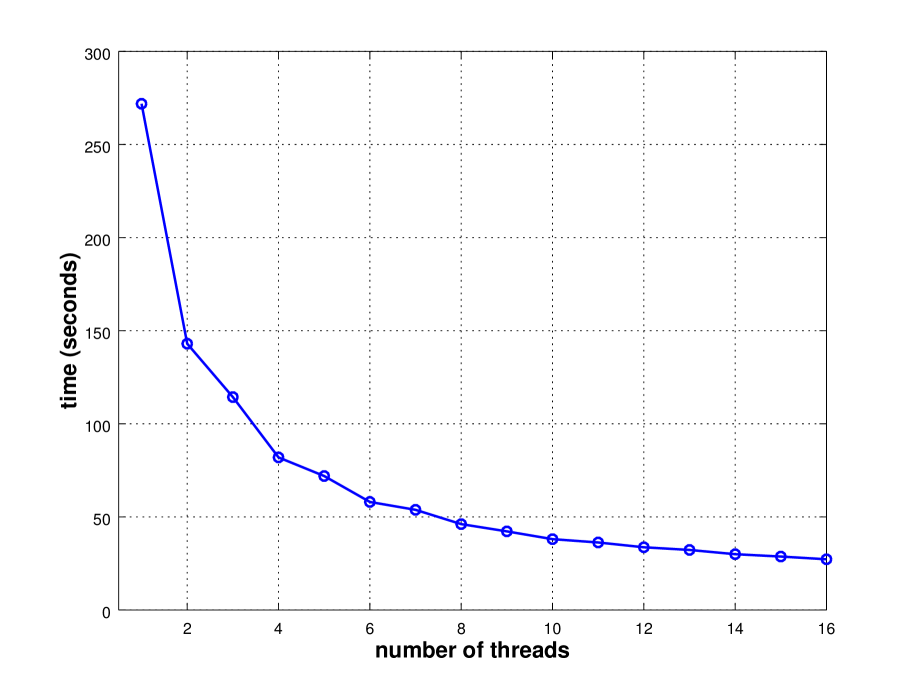
(a)

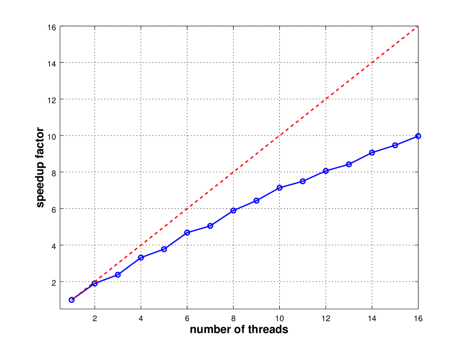
(b)

Figure 2: Execution characteristics for training a 100 component GMM to model a synthetic dataset comprising 1,000,000 samples with 100 dimensions, using 10 iterations of the k-means algorithm and 10 iterations of the EM algorithm: (a) total time taken depending on the number of threads; (b) corresponding speedup factor compared to using one thread (blue line), and idealised linear speedup under the assumption of no overheads and no memory access contention (red dotted line). The modelling was done on a machine with dual Intel Xeon E5-2620-v4 CPUs, providing 16 independent processing cores running at 2.1 GHz. Compilation was done with the GCC 5.4 C++ compiler with the following configuration options: -O3 -march=native -fopenmp.

Comparison with Full-Covariance GMMs in MLPACK

In order to validate our intuition that a diagonal GMM is a good choice instead of the significantly more complex problem of estimating GMMs with full covariance matrices, we compare the gmm_diag class (described in Section 4) against the full-covariance GMM implementation in the well-established MLPACK C++ machine learning library [6].

We selected common datasets from the UCI machine learning dataset repository [17], and trained both diagonal and full-covariance GMMs on these datasets. The number of Gaussians was chosen according to the original source of each dataset; where possible, 3 times the number of classes in the dataset was used. In some cases, small amounts of Gaussian noise was added to the dataset to ensure training stability of the full-covariance GMMs. Both implementations used 10 iterations of k-means for initialisation, followed by running the EM algorithm until convergence or reaching a maximum of 250 iterations. The entire fitting procedure was repeated 10 times, each time with a different random starting point.

The results are given in Table 1, which shows the best log-likelihood of the 10 runs, the average wall-clock runtime for the fitting, as well as dataset information (number of samples, dimensionality, and number of Gaussians used for modelling). We can see that the diagonal GMM implementation in the gmm_diag class provides speedups from one to two orders-of-magnitude over the full-covariance implementation in MLPACK. Furthermore, in most cases there is no significant loss in goodness-of-fit (as measured by log-likelihood). In several cases (winequality, phy, covertype, pokerhand) the log-likelihood is notably higher for the gmm_diag class; we conjecture that in these cases the diagonal covariance matrices are acting as a form of regularisation to reduce overfitting [3].

dataset	num.	num.	num.	MLPACK	gmm_diag	$\nicefrac{{\mbox{MLPACK}}}{{\mbox{gmm\_diag}}}$	MLPACK	gmm_diag
	samples	dims	Gaus.	fit time	fit time	fit time ratio	$\mathbf{\log}\leavevmode\nobreak\ p(X|\lambda)$	$\mathbf{\log}\leavevmode\nobreak\ p(X|\lambda)$
cloud	2,048	10	5	1.50s	0.14s	10.7	-59.98$\times$103	-64.12$\times$103
ozone	2,534	72	6	8.59s	0.10s	85.9	-226.13$\times$103	-307.95$\times$103
winequality	6,497	11	30	16.10s	0.68s	23.7	-47.12$\times$103	-15.85$\times$103
corel	37,749	32	50	544.62s	4.55s	119.7	+4.52$\times$106	+4.44$\times$106
birch3	100,000	2	6	18.13s	2.39s	7.6	-2.70$\times$106	-2.71$\times$106
phy	150,000	78	30	3867.12s	29.25s	132.2	-2.10$\times$107	-1.88$\times$107
covertype	581,012	55	21	10360.53s	64.83s	159.8	-9.46$\times$107	-6.90$\times$107
pokerhand	1,000,000	10	25	3653.94s	55.85s	65.4	-1.90$\times$107	-1.68$\times$107

Table 1: Comparison of fitting time (seconds) and goodness-of-fit (as measured by log-likelihood) using full covariance GMMs from the MLPACK library [6] against diagonal GMMs in the gmm_diag class, on common datasets from the UCI machine learning dataset repository [17]. The lower the fitting time, the better. The higher the $\log p(X|\lambda)$, the better.

Conclusion

In this paper we have demonstrated a multi-threaded and robust implementation of Gaussian Mixture Models in the C++ language. Multi-threading is achieved through reformulation of the Expectation-Maximisation and k-means algorithms into a MapReduce-like framework. The implementation also uses several techniques to improve numerical stability and improve modelling accuracy. We demonstrated that the implementation achieves a speedup of an order of magnitude on a recent 16 core machine, and that it can achieve higher modelling accuracy than a previously well-established publically accessible implementation. The multi-threaded implementation is released as open source software and included in recent releases of the cross-platform Armadillo C++ linear algebra library. The library is provided under the permissive Apache 2.0 license, allowing unencumbered use in commercial products.

Appendix A: Abridged Derivation of the EM Algorithm for Gaussian Mixture Models

In the Gaussian Mixture Model (GMM) approach, the distribution of samples (vectors) is modelled as:

$$p({\boldsymbol{x}}|\Theta)=\sum\nolimits_{m=1}^{M}w_{m}p({\boldsymbol{x}}|\theta_{m})$$ (21)

where ${\boldsymbol{x}}$ is a $D$-dimensional vector, $w_{m}$ is a weight (with constraints $\sum\nolimits_{m=1}^{M}w_{m}=1$, $w_{m}\geq 0$), and $p({\boldsymbol{x}}|\theta_{m})$ is a multivariate Gaussian density function with parameter set $\theta_{m}=\{{\boldsymbol{\mu}}_{m},{\boldsymbol{\Sigma}}_{m}\}$:

$$p({\boldsymbol{x}}|\theta_{m})={{\mathcal{N}}}({\boldsymbol{x}}|{\boldsymbol{\mu}}_{m},{\boldsymbol{\Sigma}}_{m})=\frac{1}{(2\pi)^{\frac{D}{2}}|{\boldsymbol{\Sigma}}_{m}|^{\frac{1}{2}}}\exp\left[-\frac{1}{2}({\boldsymbol{x}}-{\boldsymbol{\mu}}_{m})^{T}{\boldsymbol{\Sigma}}_{m}^{-1}({\boldsymbol{x}}-{\boldsymbol{\mu}}_{m})\right]$$ (22)

where ${\boldsymbol{\mu}}_{m}$ is the mean vector and ${\boldsymbol{\Sigma}}_{m}$ is the covariance matrix. Thus the complete parameter set for Eqn. (21) is expressed as $\Theta=\{w_{m},\theta_{m}\}_{m=1}^{M}$. Given a set of training samples, $X=\{{\boldsymbol{x}}_{i}\}_{i=1}^{N}$, we need to find $\Theta$ that suitably models the underlying distribution. Stated more formally, we need to find $\Theta$ that maximises the following likelihood function:

$$p(X|\Theta)=\prod\nolimits_{i=1}^{N}p({\boldsymbol{x}}_{i}|\Theta)$$ (23)

The Expectation-Maximisation (EM) algorithm [8, 21, 24, 27] is an iterative likelihood function optimisation technique, often used in the pattern recognition and machine learning [3, 9]. It is a general method for finding the maximum-likelihood estimate of the parameters of an assumed distribution, when either the training data is incomplete or has missing values, or when the likelihood function can be made analytically tractable by assuming the existence of (and values for) missing data.

To apply the EM algorithm to finding $\Theta$, we must first assume that our training data $X$ is incomplete and assume the existence of missing data $Y=\{y_{i}\}_{i=1}^{N}$, where each $y_{i}$ indicates the mixture component that “generated” the corresponding ${\boldsymbol{x}}_{i}$. Thus $y_{i}\in[1,M]\leavevmode\nobreak\ \forall\leavevmode\nobreak\ i$ and $y_{i}=m$ if the $i$-th feature vector (${\boldsymbol{x}}_{i}$) was “generated” by the $m$-th component. If we know the values for $Y$, then Eqn. (23) can be modified to:

$$p(X,Y|\Theta)=\prod\nolimits_{i=1}^{N}w_{y_{i}}p({\boldsymbol{x}}_{i}|\theta_{y_{i}})$$ (24)

As its name suggests, the EM algorithm is comprised of two steps which are iterated: (i) expectation, followed by (ii) maximisation. In the expectation step, the expected value of the complete data log-likelihood, $\log p(X,Y|\Theta)$, is found with respect to the unknown data $Y=\{y_{i}\}_{i=1}^{N}$ given training data $X=\{{\boldsymbol{x}}_{i}\}_{i=1}^{N}$ and current parameter estimates, $\Theta^{[k]}$ (where $k$ indicates the iteration number):

$$Q(\Theta,\Theta^{[k]})=E\left[\log p(X,Y|\Theta)\leavevmode\nobreak\ |\leavevmode\nobreak\ X,\Theta^{[k]}\right]$$ (25)

Since $Y$ is a random variable with distribution $p(\mbox{\boldmath$y$}|X,\Theta^{[k]})$, Eqn. (25) can be written as:

$$Q(\Theta,\Theta^{[k]})=\int_{\mbox{\boldmath$y$}\in\Upsilon}\log p(X,\mbox{\boldmath$y$}|\Theta)\leavevmode\nobreak\ p(\mbox{\boldmath$y$}|X,\Theta^{[k]})\leavevmode\nobreak\ \leavevmode\nobreak\ d\mbox{\boldmath$y$}$$ (26)

where $y$ is an instance of the missing data and $\Upsilon$ is the space of values $y$ can take on. The maximisation step then maximises the expectation:

$$\Theta^{[k+1]}=\arg\max_{\Theta}Q(\Theta,\Theta^{[k]})$$ (27)

The expectation and maximisation steps are iterated until convergence, or when the increase in likelihood falls below a pre-defined threshold. As can be seen in Eqn. (26), we require $p(\mbox{\boldmath$y$}|X,\Theta^{[k]})$. We can define it as follows:

$$p(\mbox{\boldmath$y$}|X,\Theta^{[k]})=\prod\nolimits_{i=1}^{N}p(y_{i}|{\boldsymbol{x}}_{i},\Theta^{[k]})$$ (28)

Given initial parameters  $\Theta^{[k]}$, we can compute $p({\boldsymbol{x}}_{i}|\theta_{m}^{[k]})$. Moreover, we can interpret the mixing weights ($w_{m}$) as a-priori probabilities of each mixture component, ie., $w_{m}=p(m|\Theta^{[k]})$. Hence we can apply Bayes’ rule [9] to obtain:

$$p(y_{i}|{\boldsymbol{x}}_{i},\Theta^{[k]}) = \frac{p({\boldsymbol{x}}_{i}|\theta_{y_{i}}^{[k]})p(y_{i}|\Theta^{[k]})}{p({\boldsymbol{x}}_{i}|\Theta^{[k]})}$$ (29)

$$= \frac{p({\boldsymbol{x}}_{i}|\theta_{y_{i}}^{[k]})p(y_{i}|\Theta^{[k]})}{\sum\nolimits_{n=1}^{M}p({\boldsymbol{x}}_{i}|\theta_{n}^{[k]})p(n|\Theta^{[k]})}$$ (30)

Expanding Eqn. (26) yields:

$$Q(\Theta,\Theta^{[k]}) = \int_{\mbox{\boldmath$y$}\in\Upsilon}\log p(X,\mbox{\boldmath$y$}|\Theta)\leavevmode\nobreak\ p(\mbox{\boldmath$y$}|X,\Theta^{[k]})\leavevmode\nobreak\ \leavevmode\nobreak\ d\mbox{\boldmath$y$}$$ (31)

$$= \sum\nolimits_{\mbox{\boldmath$y$}\in\Upsilon}\log\prod\nolimits_{i=1}^{N}w_{y_{i}}p({\boldsymbol{x}}_{i}|\theta_{y_{i}})\prod\nolimits_{j=1}^{N}p(y_{j}|{\boldsymbol{x}}_{j},\Theta^{[k]})$$ (32)

$$= \sum\nolimits_{y_{1}=1}^{M}\sum\nolimits_{y_{2}=1}^{M}\cdots\sum\nolimits_{y_{N}=1}^{M}\sum\nolimits_{i=1}^{N}\log\left[w_{y_{i}}p({\boldsymbol{x}}_{i}|\theta_{y_{i}})\right]\prod\nolimits_{j=1}^{N}p(y_{j}|{\boldsymbol{x}}_{j},\Theta^{[k]})$$ (33)

It can be shown [2] that Eqn. (33) can be simplified to:

$$Q(\Theta,\Theta^{[k]}) = \sum\nolimits_{m=1}^{M}\sum\nolimits_{i=1}^{N}\log[w_{m}p({\boldsymbol{x}}_{i}|\theta_{m})]\leavevmode\nobreak\ p(m|{\boldsymbol{x}}_{i},\Theta^{[k]})$$ (34)

$$= \sum\nolimits_{m=1}^{M}\sum\nolimits_{i=1}^{N}\log[w_{m}]\leavevmode\nobreak\ p(m|{\boldsymbol{x}}_{i},\Theta^{[k]})+\sum\nolimits_{m=1}^{M}\sum\nolimits_{i=1}^{N}\log[p({\boldsymbol{x}}_{i}|\theta_{m})]\leavevmode\nobreak\ p(m|{\boldsymbol{x}}_{i},\Theta^{[k]})\leavevmode\nobreak\ \leavevmode\nobreak\ \leavevmode\nobreak\$$ (35)

$$= Q_{1}\leavevmode\nobreak\ \leavevmode\nobreak\ \leavevmode\nobreak\ +\leavevmode\nobreak\ \leavevmode\nobreak\ \leavevmode\nobreak\ Q_{2}$$ (36)

Hence $Q_{1}$ and $Q_{2}$ can be maximised separately, to obtain $w_{m}$ and $\theta_{m}=\{{\boldsymbol{\mu}}_{m},{\boldsymbol{\Sigma}}_{m}\}$, respectively. To find the expression which maximises $w_{m}$, we need to introduce the Lagrange multiplier [9] $\psi$, with the constraint $\sum\nolimits_{m}w_{m}=1$, take the derivative of $Q_{1}$ with respect to $w_{m}$ and set the result to zero:

$$\frac{\partial Q_{1}}{\partial w_{m}} = 0$$ (37)

$$\therefore\leavevmode\nobreak\ 0 = \frac{\partial}{\partial w_{m}}\left\{\sum\nolimits_{m=1}^{M}\sum\nolimits_{i=1}^{N}\log[w_{m}]\leavevmode\nobreak\ p(m|{\boldsymbol{x}}_{i},\Theta^{[k]})+\psi\left[(\sum\nolimits_{m}w_{m})-1\right]\right\}$$ (38)

$$= \sum\nolimits_{i=1}^{N}\frac{1}{w_{m}}\leavevmode\nobreak\ p(m|{\boldsymbol{x}}_{i},\Theta^{[k]})+\psi$$ (39)

Rearranging Eqn. (39) to obtain a value for $\psi$:

$$-\psi w_{m} = \sum\nolimits_{i=1}^{N}p(m|{\boldsymbol{x}}_{i},\Theta^{[k]})$$ (40)

Summing both sides over $m$ yields:

$$-\psi\sum\nolimits_{m}w_{m} = \sum\nolimits_{i=1}^{N}\sum\nolimits_{m}p(m|{\boldsymbol{x}}_{i},\Theta^{[k]})$$ (41)

$$-\psi 1 = \sum\nolimits_{i=1}^{N}1$$ (42)

$$\psi = -N$$ (43)

By substituting Eqn. (43) into Eqn. (39) we obtain:

$$N = \sum\nolimits_{i=1}^{N}\frac{1}{w_{m}}\leavevmode\nobreak\ p(m|{\boldsymbol{x}}_{i},\Theta^{[k]})$$ (44)

$$\therefore\leavevmode\nobreak\ w_{m} = \frac{1}{N}\sum\nolimits_{i=1}^{N}p(m|{\boldsymbol{x}}_{i},\Theta^{[k]})$$ (45)

To find expressions which maximise ${\boldsymbol{\mu}}_{m}$ and ${\boldsymbol{\Sigma}}_{m}$, let us now expand $Q_{2}$:

$$Q_{2} = \sum\nolimits_{m=1}^{M}\sum\nolimits_{i=1}^{N}\log[p({\boldsymbol{x}}_{i}|\theta_{m})]\leavevmode\nobreak\ p(m|{\boldsymbol{x}}_{i},\Theta^{[k]})$$ (46)

$$= \sum\nolimits_{m=1}^{M}\sum\nolimits_{i=1}^{N}\left[-\frac{1}{2}\log(|{\boldsymbol{\Sigma}}_{m}|)-\frac{1}{2}({\boldsymbol{x}}_{i}-{\boldsymbol{\mu}}_{m})^{T}{\boldsymbol{\Sigma}}_{m}^{-1}({\boldsymbol{x}}_{i}-{\boldsymbol{\mu}}_{m})\right]p(m|{\boldsymbol{x}}_{i},\Theta^{[k]})$$ (47)

where $-\frac{D}{2}\log(2\pi)$ was omitted since it vanishes when taking a derivative with respect to ${\boldsymbol{\mu}}_{m}$ or ${\boldsymbol{\Sigma}}^{-1}_{m}$. To find the expression which maximises ${\boldsymbol{\mu}}_{m}$, we need to take the derivative of $Q_{2}$ with respect to ${\boldsymbol{\mu}}_{m}$, and set the result to zero:

$$\frac{\partial Q_{2}}{\partial{\boldsymbol{\mu}}_{m}} = 0$$ (48)

$$0 = \frac{\partial}{\partial{\boldsymbol{\mu}}_{m}}\left\{\sum\nolimits_{m=1}^{M}\sum\nolimits_{i=1}^{N}\left[-\frac{1}{2}\log(|\Sigma_{m}|)-\frac{1}{2}({\boldsymbol{x}}_{i}-{\boldsymbol{\mu}}_{m})^{T}{\boldsymbol{\Sigma}}_{m}^{-1}({\boldsymbol{x}}_{i}-{\boldsymbol{\mu}}_{m})\right]p(m|{\boldsymbol{x}}_{i},\Theta^{[k]})\right\}\leavevmode\nobreak\ \leavevmode\nobreak\ \leavevmode\nobreak\ \leavevmode\nobreak\ \leavevmode\nobreak\ \leavevmode\nobreak\ \leavevmode\nobreak\ \leavevmode\nobreak\ \leavevmode\nobreak\$$ (49)

Lütkepohl [19] states that $\frac{\partial{\boldsymbol{z}}^{T}{\boldsymbol{A}}{\boldsymbol{z}}}{\partial{\boldsymbol{z}}}=({\boldsymbol{A}}+{\boldsymbol{A}}^{T}){\boldsymbol{z}}$,   $({\boldsymbol{A}}^{-1})^{T}=({\boldsymbol{A}}^{T})^{-1}$ and if ${\boldsymbol{A}}$ is symmetric, then ${\boldsymbol{A}}={\boldsymbol{A}}^{T}$. Since ${\boldsymbol{\Sigma}}_{m}$ is symmetric, Eqn. (49) reduces to:

$$0 = \sum\nolimits_{i=1}^{N}-\frac{1}{2}2{\boldsymbol{\Sigma}}_{m}^{-1}({\boldsymbol{x}}_{i}-{\boldsymbol{\mu}}_{m})p(m|{\boldsymbol{x}}_{i},\Theta^{[k]})$$ (50)

$$= \sum\nolimits_{i=1}^{N}\left[-{\boldsymbol{\Sigma}}_{m}^{-1}{\boldsymbol{x}}_{i}p(m|{\boldsymbol{x}}_{i},\Theta^{[k]})+{\boldsymbol{\Sigma}}_{m}^{-1}{\boldsymbol{\mu}}_{m}p(m|{\boldsymbol{x}}_{i},\Theta^{[k]})\right]\leavevmode\nobreak\ \leavevmode\nobreak\ \leavevmode\nobreak\$$ (51)

$$\therefore\leavevmode\nobreak\ \sum\nolimits_{i=1}^{N}{\boldsymbol{\Sigma}}_{m}^{-1}{\boldsymbol{\mu}}_{m}p(m|{\boldsymbol{x}}_{i},\Theta^{[k]}) = \sum\nolimits_{i=1}^{N}{\boldsymbol{\Sigma}}_{m}^{-1}{\boldsymbol{x}}_{i}p(m|{\boldsymbol{x}}_{i},\Theta^{[k]})$$ (52)

Multiplying both sides by ${\boldsymbol{\Sigma}}_{m}$ yields:

$$\sum\nolimits_{i=1}^{N}{\boldsymbol{\mu}}_{m}p(m|{\boldsymbol{x}}_{i},\Theta^{[k]}) = \sum\nolimits_{i=1}^{N}{\boldsymbol{x}}_{i}p(m|{\boldsymbol{x}}_{i},\Theta^{[k]})$$ (53)

$$\therefore\leavevmode\nobreak\ {\boldsymbol{\mu}}_{m} = \frac{\sum\nolimits_{i=1}^{N}{\boldsymbol{x}}_{i}p(m|{\boldsymbol{x}}_{i},\Theta^{[k]})}{\sum\nolimits_{i=1}^{N}p(m|{\boldsymbol{x}}_{i},\Theta^{[k]})}$$ (54)

Lütkepohl [19] states that: $|{\boldsymbol{A}}^{-1}|=|{\boldsymbol{A}}|^{-1}$ and $\mbox{tr}({\boldsymbol{A}}{\boldsymbol{B}})=\mbox{tr}({\boldsymbol{B}}{\boldsymbol{A}})$. Since $\mbox{tr}{({\boldsymbol{z}}A{\boldsymbol{z}}^{T})}=\mbox{tr}(\mbox{scalar})$, we can rewrite Eqn. (47) as:

$$Q_{2} = \sum\nolimits_{m=1}^{M}\sum\nolimits_{i=1}^{N}\left[\frac{1}{2}\log(|{\boldsymbol{\Sigma}}_{m}^{-1}|)-\frac{1}{2}\mbox{tr}({\boldsymbol{\Sigma}}_{m}^{-1}({\boldsymbol{x}}_{i}-{\boldsymbol{\mu}}_{m})({\boldsymbol{x}}_{i}-{\boldsymbol{\mu}}_{m})^{T})\right]p(m|{\boldsymbol{x}}_{i},\Theta^{[k]})$$ (55)

According to Lütkepohl [19], $\frac{\partial\log(|{\boldsymbol{A}}|)}{\partial{\boldsymbol{A}}}=({\boldsymbol{A}}^{T})^{-1}$ and $\frac{\partial\mbox{tr}({\boldsymbol{B}}{\boldsymbol{A}})}{\partial{\boldsymbol{B}}}={\boldsymbol{A}}^{T}$. Moreover, we note that ${\boldsymbol{z}}{\boldsymbol{z}}^{T}$ is a symmetric matrix. To find an expression which maximises ${\boldsymbol{\Sigma}}_{m}$, we can take the derivative of Eqn. (55) with respect to ${\boldsymbol{\Sigma}}_{m}^{-1}$ and set the result to zero:

$$0 = \frac{\partial Q_{2}}{\partial{\boldsymbol{\Sigma}}_{m}^{-1}}$$ (56)

$$= \frac{\partial}{\partial{\boldsymbol{\Sigma}}_{m}^{-1}}\left\{\sum\nolimits_{m=1}^{M}\sum\nolimits_{i=1}^{N}\left[\frac{1}{2}\log(|{\boldsymbol{\Sigma}}_{m}^{-1}|)-\frac{1}{2}\mbox{tr}\left({\boldsymbol{\Sigma}}_{m}^{-1}({\boldsymbol{x}}_{i}-{\boldsymbol{\mu}}_{m})({\boldsymbol{x}}_{i}-{\boldsymbol{\mu}}_{m})^{T}\right)\right]p(m|{\boldsymbol{x}}_{i},\Theta^{[k]})\right\}$$ (57)

$$= \sum\nolimits_{i=1}^{N}\left[\frac{1}{2}{\boldsymbol{\Sigma}}_{m}-\frac{1}{2}({\boldsymbol{x}}_{i}-{\boldsymbol{\mu}}_{m})({\boldsymbol{x}}_{i}-{\boldsymbol{\mu}}_{m})^{T}\right]p(m|{\boldsymbol{x}}_{i},\Theta^{[k]})$$ (58)

thus

$$\frac{1}{2}{\boldsymbol{\Sigma}}_{m}\sum\nolimits_{i=1}^{N}p(m|{\boldsymbol{x}}_{i},\Theta^{[k]}) = \frac{1}{2}\sum\nolimits_{i=1}^{N}({\boldsymbol{x}}_{i}-{\boldsymbol{\mu}}_{m})({\boldsymbol{x}}_{i}-{\boldsymbol{\mu}}_{m})^{T}p(m|{\boldsymbol{x}}_{i},\Theta^{[k]})$$ (60)

$$\therefore\leavevmode\nobreak\ {\boldsymbol{\Sigma}}_{m} = \frac{\sum\nolimits_{i=1}^{N}({\boldsymbol{x}}_{i}-{\boldsymbol{\mu}}_{m})({\boldsymbol{x}}_{i}-{\boldsymbol{\mu}}_{m})^{T}p(m|{\boldsymbol{x}}_{i},\Theta^{[k]})}{\sum\nolimits_{i=1}^{N}p(m|{\boldsymbol{x}}_{i},\Theta^{[k]})}$$ (61)

In summary,

$$w_{m}^{[k+1]} = \frac{1}{N}\sum\nolimits_{i=1}^{N}p(m|{\boldsymbol{x}}_{i},\Theta^{[k]})$$ (62)

$${\boldsymbol{\mu}}_{m}^{[k+1]} = \frac{\sum\nolimits_{i=1}^{N}{\boldsymbol{x}}_{i}\leavevmode\nobreak\ p(m|{\boldsymbol{x}}_{i},\Theta^{[k]})}{\sum\nolimits_{i=1}^{N}p(m|{\boldsymbol{x}}_{i},\Theta^{[k]})}$$ (63)

$${\boldsymbol{\Sigma}}_{m}^{[k+1]} = \frac{\sum\nolimits_{i=1}^{N}({\boldsymbol{x}}_{i}-{\boldsymbol{\mu}}_{m}^{[k+1]})({\boldsymbol{x}}_{i}-{\boldsymbol{\mu}}_{m}^{[k+1]})^{T}p(m|{\boldsymbol{x}}_{i},\Theta^{[k]})}{\sum\nolimits_{i=1}^{N}p(m|{\boldsymbol{x}}_{i},\Theta^{[k]})}$$ (64)

where

$$p(m|{\boldsymbol{x}}_{i},\Theta^{[k]})=\frac{p({\boldsymbol{x}}_{i}|\theta_{m}^{[k]})p(m|\Theta^{[k]})}{\sum\nolimits_{n=1}^{M}p({\boldsymbol{x}}_{i}|\theta_{n}^{[k]})p(n|\Theta^{[k]})}$$ (65)

which can be explicitly stated as:

$$p(m|{\boldsymbol{x}}_{i},\Theta^{[k]})=\frac{{\mathcal{N}}({\boldsymbol{x}}_{i}|{\boldsymbol{\mu}}_{m}^{[k]},{\boldsymbol{\Sigma}}_{m}^{[k]})w_{m}^{[k]}}{\sum\nolimits_{n=1}^{M}{\mathcal{N}}({\boldsymbol{x}}_{i}|{\boldsymbol{\mu}}_{n}^{[k]},{\boldsymbol{\Sigma}}_{n}^{[k]})w_{n}^{[k]}}$$ (66)

If we let $l_{m,i}=p(m|{\boldsymbol{x}}_{i},\Theta^{[k]})$ and $L_{m}=\sum\nolimits_{i=1}^{N}l_{m,i}$, we can restate Eqns. (62) to (64) as:

$$w_{m}^{[k+1]} = \frac{L_{m}}{N}$$ (67)

$${\boldsymbol{\mu}}_{m}^{[k+1]} = \frac{1}{L_{m}}\sum\nolimits_{i=1}^{N}{\boldsymbol{x}}_{i}\leavevmode\nobreak\ l_{m,i}$$ (68)

$${\boldsymbol{\Sigma}}_{m}^{[k+1]} = \frac{1}{L_{m}}\sum\nolimits_{i=1}^{N}({\boldsymbol{x}}_{i}-{\boldsymbol{\mu}}_{m}^{[k+1]})({\boldsymbol{x}}_{i}-{\boldsymbol{\mu}}_{m}^{[k+1]})^{T}l_{m,i}$$ (69)

References

- [1] D. Arthur and S. Vassilvitskii. k-means++: the advantages of careful seeding. In ACM-SIAM Symposium on Discrete Algorithms, pages 1027–1035, 2007.
- [2] J. Bilmes. A gentle tutorial of the EM algorithm and its applications to parameter estimation for Gaussian mixture and hidden Markov models. Technical Report TR-97-021, International Computer Science Institute, Berkeley, California, 1998.
- [3] C. Bishop. Pattern Recognition and Machine Learning. Springer, 2006.
- [4] J. Carvajal, A. Wiliem, C. McCool, B. Lovell, and C. Sanderson. Comparative evaluation of action recognition methods via Riemannian manifolds, Fisher vectors and GMMs: Ideal and challenging conditions. In Lecture Notes in Computer Science (LNCS), Vol. 9794, pages 88–100, 2016.
- [5] B. Chapman, G. Jost, and R. van der Pas. Using OpenMP: Portable Shared Memory Parallel Programming. MIT Press, 2007.
- [6] R. R. Curtin, J. R. Cline, N. P. Slagle, W. B. March, P. Ram, N. A. Mehta, and A. G. Gray. MLPACK: A scalable C++ machine learning library. Journal of Machine Learning Research, 14:801–805, 2013.
- [7] J. Dean and S. Ghemawat. MapReduce: Simplified data processing on large clusters. In Symposium on Operating Systems Design and Implementation, pages 137–150, 2004.
- [8] A. Dempster, N. Laird, and D. Rubin. Maximum likelihood from incomplete data via the EM algorithm. Journal of the Royal Statistical Society, Series B (Methodological), 39(1):1–38, 1977.
- [9] R. Duda, P. Hart, and D. Stork. Pattern Classification. John Wiley & Sons, 2001.
- [10] C. Elkan. Using the triangle inequality to accelerate k-means. In International Conference on Machine Learning, pages 147–153, 2003.
- [11] Z. Ge, C. McCool, C. Sanderson, and P. Corke. Modelling local deep convolutional neural network features to improve fine-grained image classification. In International Conference on Image Processing (ICIP), pages 4112–4116, 2015.
- [12] Z. Ge, C. McCool, C. Sanderson, P. Wang, L. Liu, I. Reid, and P. Corke. Exploiting temporal information for DCNN-based fine-grained object classification. In International Conference on Digital Image Computing: Techniques and Applications, 2016.
- [13] D. Goldberg. What every computer scientist should know about floating-point arithmetic. ACM Computing Surveys, 23(1):5–48, 1991.
- [14] G. Hamerly and C. Elkan. Learning the k in k-means. In Neural Information Processing Systems, 2003.
- [15] B. Kulis and M. I. Jordan. Revisiting k-means: New algorithms via Bayesian nonparametrics. In International Conference on Machine Learning, pages 513–520, 2012.
- [16] Y. LeCun, Y. Bengio, and G. Hinton. Deep learning. Nature, 521:436–444, 2015.
- [17] M. Lichman. UCI machine learning repository, 2013. http://archive.ics.uci.edu/ml.
- [18] Y. Linde, A. Buzo, and R. Gray. An algorithm for vector quantization. IEEE Transactions on Communications, 28(1):84–95, 1980.
- [19] H. Lütkepohl. Handbook of Matrices. John Wiley & Sons, 1996.
- [20] M. McCool, J. Reinders, and A. Robison. Structured Parallel Programming: Patterns for Efficient Computation. Morgan Kaufmann, 2012.
- [21] G. McLachlan and T. Krishnan. The EM Algorithm and Extensions. John Wiley & Sons, 2nd edition, 2008.
- [22] T. Mitchell. Machine Learning. McGraw-Hill, 1997.
- [23] D. Monniaux. The pitfalls of verifying floating-point computations. ACM Transactions on Programming Languages and Systems, 30(3), 2008.
- [24] T. Moon. Expectation-maximization algorithm. IEEE Signal Processing Magazine, 13(6):47–60, 1996.
- [25] D. Pelleg and A. Moore. X-means: Extending K-means with efficient estimation of the number of clusters. In International Conference on Machine Learning, pages 727–734, 2000.
- [26] V. Reddy, C. Sanderson, and B. Lovell. Improved foreground detection via block-based classifier cascade with probabilistic decision integration. IEEE Transactions on Circuits and Systems for Video Technology, 23(1):83–93, 2013.
- [27] R. Redner and H. F. Walker. Mixture densities, maximum likelihood and the EM algorithm. SIAM Review, 26(2):195–239, 1984.
- [28] D. Reynolds, T. Quatieri, and R. Dunn. Speaker verification using adapted Gaussian mixture models. Digital Signal Processing, 10(1–3):19–41, 2000.
- [29] C. Sanderson and R. Curtin. Armadillo: a template-based C++ library for linear algebra. Journal of Open Source Software, 1:26, 2016.
- [30] C. Sanderson and R. Curtin. Armadillo: C++ template metaprogramming for compile-time optimization of linear algebra. In Platform for Advanced Scientific Computing (PASC) Conference, Switzerland, 2017.
- [31] A. St. Laurent. Understanding Open Source and Free Software Licensing. O’Reilly Media, 2008.
- [32] A. Wiliem, C. Sanderson, Y. Wong, P. Hobson, R. Minchin, and B. Lovell. Automatic classification of human epithelial type 2 cell indirect immunofluorescence images using cell pyramid matching. Pattern Recognition, 47(7):2315–2324, 2014.
- [33] Y. Wong, M. Harandi, and C. Sanderson. On robust face recognition via sparse coding: The good, the bad and the ugly. IET Biometrics, 3(4):176–189, 2014.