The $\alpha+d\rightarrow~{}^{6}\mathrm{Li}+\gamma$ astrophysical $S$-factor and its implications for Big Bang Nucleosynthesis

Abstract

The $\alpha+d\rightarrow\,^{6}{\rm Li}+\gamma$ radiative capture is studied in order to predict the ⁶Li primordial abundance. Within a two-body framework, the $\alpha$ particle and the deuteron are considered the structureless constituents of ⁶Li . Five $\alpha+d$ potentials are used to solve the two-body problem: four of them are taken from the literature, only one having also a tensor component. A fifth model is here constructed in order to reproduce, besides the ⁶Li static properties as binding energy, magnetic dipole and electric quadrupole moments, also the $S$-state asymptotic normalization coefficient (ANC). The two-body bound and scattering problem is solved with different techniques, in order to minimize the numerical uncertainty of the present results. The long-wavelength approximation is used, and therefore only the electric dipole and quadrupole operators are retained. The astrophysical $S$-factor is found to be significantly sensitive to the ANC, but in all the cases in good agreement with the available experimental data. The theoretical uncertainty has been estimated of the order of few % when the potentials which reproduce the ANC are considered, but increases up to $\simeq 20$% when all the five potential models are retained. The effect of this $S$-factor prediction on the ⁶Li primordial abundance is studied, using the public code PArthENoPE. For the five models considered here we find ${}^{6}{\rm Li}/$H$=(0.9-1.8)\times 10^{-14}$, with the baryon density parameter in the 3-$\sigma$ range of Planck 2015 analysis, $\Omega_{b}h^{2}=0.02226\pm 0.00023$.

I Introduction

The $\alpha+d$ radiative capture

$$\alpha+d\rightarrow^{6}{\rm Li}+\gamma$$ (1)

has recently received quite some interest, triggered by the so-called ⁶Li problem. In the theory of Big Bang Nucleosynthesis (BBN), even if it is a weak electric quadrupole transition, this reaction is important as represents the main ⁶Li production process. In 2006 Asplund et al. performed high resolution observations of Li absorption lines in old halo stars asp06 . The ⁶Li/⁷Li ratio was found to be of about $5\times 10^{-2}$, more than two orders of magnitude larger than the expected BBN prediction. Since the analysis is performed on old stars, the quantity of the present ⁶Li should be a good estimate of the one at the star formation, i.e. the same after BBN. This great discrepancy is the so-called second Lithium problem. However, recent analyses with three-dimensional modelling of stellar atmosphere, which do not assume local thermodynamical equilibrium and include surface convection effects, show that these can explain the observed line asymmetry. The ${}^{6}\rm{Li}$ problem, therefore, would be weakened cayrel ; perez ; steffen ; lind .

We recall that the BBN relevant energy window is located between 50 and 400 keV, and experimental studies of Eq. (1) at these energies are very difficult, due to the exponential drop of the reaction cross section as a consequence of the Coulomb barrier. Furthermore, this reaction is affected by the isotopic suppression of the electric dipole operator, as it will be discussed in Sec. II.2. The reaction (1) was first studied experimentally in the early 1980s rob81 and then thorough the 1990s kie91 ; moh94 ; cec96 ; iga00 . However the data in the BBN energy range were affected by large uncertainties. The latest measurement is that performed by the LUNA Collaboration and14 ; tre17 .

The theoretical study of this reaction is also very difficult, since, in principle, we should solve a six-body problem, i.e. we should consider the six nucleons contained in the $\alpha+d$ and ⁶Li particles, and their interaction with the photon. Such an approach is known as the ab-initio method, and it has been used only by Nollett et al. in Ref. nol01 . However, the numerical techniques used in Ref. nol01 to solve the six-body problem, i.e. the variational Monte Carlo method, provide solutions for the initial and final state wave functions with uncertainties at the 10-20% level. Since ab-initio methods are still nowadays hardly implemented for $A>4$ radiative captures, the study of the reaction has been done using a simplified model, where ⁶Li is seen as an $\alpha+d$ system and the problem is reduced to a two-body problem. Then a crucial input for the calculation is represented by the potential model, which describes the $\alpha+d$ interaction. Five different potential models have been considered in this work, four of them taken from Refs. ham10 ; tur15 ; muk11 ; dub98 , and a last one constructed here starting from the model of Ref. dub98 , and then modifying it in order to reproduce the asymptotic normalization coefficient (ANC), i.e. the ratio between the $\alpha+d$ relative radial wave function in ⁶Li and the Whittaker function for large distances. It describes the bound-state wave function in the asymptotic region. To be noticed that only the potential of Ref. dub98 and this last model have a tensor component, necessary to describe the experimental values for the ⁶Li magnetic dipole and electric quadrupole moments. Our calculations have been performed using two methods to solve the two-body Schrödinger equation, both for the bound and the scattering states, in order to verify that our results are not affected by significant numerical uncertainties.

The paper is organized as follows: in Sec. II we introduce all the main ingredients of the present calculation for the astrophysical $S$-factor and we present in Sec. II.3 our results. In Sec. III we discuss the implications of the present calculated $S$-factor for the BBN prediction of ⁶Li abundance. We give our final remarks in Sec. IV.

II The $\alpha+d$ S-factor

The $\alpha+d$ astrophysical $S$-factor $S(E)$, $E$ being the initial center-of-mass energy, is defined as

$$S(E)=E\sigma(E)\exp(2\pi\eta)\>,$$ (2)

where $\sigma(E)$ is the capture cross section, and $\eta=2\alpha/v_{\rm rel}$ is the Sommerfeld parameter, $\alpha$ being the fine structure constant and $v_{\rm rel}$ the $\alpha+d$ relative velocity. With this definition, the $S$-factor has a smooth dependence on $E$ and can be easily extrapolated at low energies of astrophysical interest. The reaction cross section $\sigma(E)$ is given by

$$\sigma(E)=\int{\mathrm{d}}\Omega_{\hat{\bf q}}\frac{{\mathrm{d}}\sigma}{{\mathrm{d}}\Omega_{\hat{\bf q}}}\>,$$ (3)

where the differential cross section ${\mathrm{d}}\sigma/{\mathrm{d}}\Omega_{\hat{\bf q}}$ can be written as

$$\frac{\mathrm{d}\sigma}{\mathrm{d}\Omega_{\hat{\bf{q}}}}=\frac{e^{2}}{24\pi^{2}v_{rel}}\frac{q}{1+q/m_{6}}\sum_{M_{i}\lambda M}\left|\hat{\epsilon}^{\dagger\lambda}_{\mathbf{q}}\cdot\left\langle\Psi_{{}^{6}\mathrm{Li}}(M)|\mathbf{J}^{\dagger}(\mathbf{q})|\Psi_{\alpha d}(M_{i})\right\rangle\right|^{2}\>.$$ (4)

Here $m_{6}$ is the ⁶Li mass, ${\bf q}$ is the photon momentum and $\hat{\epsilon}^{\dagger\lambda}_{\mathbf{q}}$ its polarization vector, $\mathbf{J}^{\dagger}(\mathbf{q})$ is the Fourier transform of the nuclear electromagnetic current, and $\Psi_{\alpha d}(M_{i})$ and $\Psi_{{}^{6}\mathrm{Li}}(M)$ are the initial $\alpha+d$ and final ⁶Li wave functions, with spin projection $M_{i}$ and $M$. In Eq. (4), we have averaged over the initial spin projections and summed over the final ones.

In order to calculate the $\alpha+d$ cross section, it is necessary to evaluate the ⁶Li and $\alpha+d$ wave functions. This point is described in the next Subsection.

II.1 The ⁶Li and $\alpha+d$ systems

A crucial input for our calculation is represented by the ⁶Li and $\alpha+d$ wave functions. We consider first the bound state. The nucleus of ⁶Li has $J^{\pi}=1^{+}$, a binding energy $B$ respect to the $\alpha+d$ threshold of 1.475 MeV dub98 , a non-null electric quadrupole moment $Q_{6}=-0.0644(7)$ fm² and a magnetic dipole moment $\mu_{6}=-0.822$ $\mu_{N}$ dub98 . As it was shown in Ref. muk11 , the astrophysical $S$-factor at low energies is highly sensitive not only to the ⁶Li binding energy $B$ and the $\alpha+d$ scattering phase shifts, but also to the ⁶Li $S$-state asymptotic normalization coefficient (ANC). This quantity is crucial due to the peripheral nature of the $\alpha+d$ reaction at low energies, where only the tail of the ⁶Li wave function gives most of the contribution in the matrix element of Eq. (4). The $S$-state ANC is defined as

$$C_{\ell=0}=\lim_{r\rightarrow+\infty}\frac{\varphi(r)}{W_{-\eta,\ell+1/2}(r)}\bigg{|}_{\ell=0}\>,$$ (5)

where $\varphi(r)$ is the $S$-state ⁶Li reduced wave function, $W_{-\eta,\ell+1/2}(r)$ is the Whittaker function, $\eta$ is the Sommerfeld factor and $\ell=0$ for the $S$-state ANC. Its experimental value for ⁶Li is ANC${}_{\rm exp}=(2.30\pm 0.12)$ fm^1/2 tur15 .

In the present study we consider the ⁶Li nucleus as a compound system, made of an $\alpha$ particle and a deuteron. In fact, as it was shown in Ref. dub94 , the $\alpha+d$ clusterization percentage in ⁶Li can be up to about 60-80%. Therefore, we solve in this work a two-body problem, including both $S-$ and $D$-states in the $\alpha+d$ bound system. The first observable that we will try to reproduce is the binding energy, but we will consider also the above mentioned observables of ⁶Li .

At this point, an important input for the calculation is represented by the $\alpha+d$ potential. The different models considered in this work will be discussed below.

II.1.1 The $\alpha+d$ Potentials

For our calculation we consider five different potential models. The use of so many models allows us to get a hint on the theoretical uncertainty arising from the description of the ⁶Li nucleus and the $\alpha+d$ scattering system. Four of these potentials are taken from Refs. ham10 ; muk11 ; tur15 ; dub98 , while the last one has been constructed in the present work as described below. The physical constants present in each potential as listed on the original references are summarized in Table 1.

	units	$V_{H}$ and $V_{M}$	$V_{T}$, $V_{D}$ and $V_{G}$
$A_{d}$	-	2.01411	2
$A_{\alpha}$	-	4.00260	4
$m_{u}$	MeV	931.494043	938.973881
$\mu$	MeV	1248.09137	1251.96518
$\hbar^{2}/2\mu$	MeV fm2	15.5989911176	15.5507250000
$\alpha$	-	7.297352568$\times$103	7.297405999$\times$103
$\alpha\hbar c$	MeV fm	1.4399644567	1.4399750000
$B$	MeV	1.474	1.475 ($V_{T}$)
			1.4735 ($V_{D}$ and $V_{G}$)

Table 1: Set of the constants present in the five $\alpha+d$ potential models, labelled as $V_{H}$, $V_{T}$, $V_{M}$, $V_{D}$, taken from Refs. ham10 ; tur15 ; muk11 ; dub98 , respectively, and $V_{G}$, constructed in the present work. $A_{\alpha}$ ($A_{d}$) is the mass numbers of the $\alpha$ ($d$) particle, $m_{u}$ is the mass unit, equal to the atomic mass unit for $V_{H}$ and $V_{M}$, and to the average nucleon mass for $V_{T}$, $V_{D}$ and $V_{G}$, $\mu$ is the $\alpha+d$ reduced mass, $\alpha$ is the fine-structure constant and $B$ is the ⁶Li binding energy respect to the $\alpha+d$ threshold. The underlined quantities are deduced from other data given by the authors in the original references ham10 ; tur15 ; muk11 ; dub98 .

The first potential used in our study has been taken from Ref. ham10 and has the form

$$V_{H}(r)=-V_{C}^{\ell}\left[1+\exp\left(\frac{r-r_{0}}{a}\right)\right]^{-1}+V_{SO}\frac{\lambda^{2}\mathbf{L}\cdot\mathbf{S}}{r}\frac{\mathrm{d}}{\mathrm{d}r}\left[1+\exp\left(\frac{r-r_{0}}{a}\right)\right]^{-1}+V_{Coul}^{(m)}(r)\>.$$ (6)

It contains a spin-independent Wood-Saxon component, a spin-orbit interaction term, and a modified Coulomb potential, which is written as

$$V_{Coul}^{(m)}(r)=Z_{\alpha}Z_{d}\>\alpha\>\left\{\begin{array}[]{ll}\left[3-\left(r/r_{0}\right)^{2}\right]/\left(2r_{0}\right)&\mbox{if }r\leq r_{0}\\ 1/r&\mbox{if }r>r_{0}\end{array}\right.\>.$$ (7)

The values for all the parameters present in Eqs. (6) and (7), as well as those of the following potentials, are listed in Table 2, apart from $r_{0}$, which is $r_{0}=1.25\,A^{1/3}$ fm, with $A=6$. To be noticed that this potential does not reproduce the experimental value of the ANC, as it has been noticed in Ref. muk11 , and we have ourselves verified by calculating the ⁶Li properties (see below).

The second potential is taken from Ref. tur15 , and can be written as

$$V_{T}(r)=-V_{0}^{\ell}\exp\left(-\frac{r^{2}}{a_{\ell}^{2}}\right)+V_{Coul}(r)\>.$$ (8)

It is therefore the sum of a Gaussian function and a Coulomb point-like interaction $V_{Coul}(r)=Z_{\alpha}Z_{d}\>\alpha/r$. It reproduces the experimental ANC for the ⁶Li (see below).

The third potential is obtained by adding to the $V_{H}$ potential of Ref. ham10 , a new term $V_{N}(r)$, such that the new potential

$$V_{M}(r)=V_{H}(r)+V_{N}(r)$$ (9)

reproduces the experimental ANC muk11 . The procedure to obtain $V_{N}(r)$ is discussed at length in Ref. muk11 . Here we have generalized it to the coupled-channel case, and it will be discussed below.

The potentials $V_{H}$, $V_{T}$ and $V_{M}$ considered so far are central potentials, which have, at maximum, a spin-orbit term. Therefore, these potentials are unable to give rise to the ${}^{3}D_{1}$ component in the ⁶Li wave function. The non-zero ⁶Li quadrupole moment has induced us to consider also potentials which include a tensor term. In this study, we have used the potential of Ref. dub98 , which can be written as

$$V_{D}(r)=-V_{0}^{\ell J}\exp\left(-\frac{r^{2}}{a^{2}}\right)-V_{1}^{\ell}\exp\left(-\frac{r^{2}}{b^{2}}\right)\left[6\frac{(\mathbf{S}\cdot\mathbf{r})^{2}}{r^{2}}-2\mathbf{S^{2}}\right]+V_{Coul}(r)\>,$$ (10)

where $\mathbf{S}$ is the spin operator acting on ⁶Li. The coefficients $V_{0}^{\ell J}\equiv V_{0}^{01}$ and $V_{0}^{\ell J}\equiv V_{0}^{21}$ have been taken from Ref. dub98 . However, in Ref. dub98 this potential was used only for the bound-state problem. Therefore, we have modified the potential in order to reproduce also the scattering phase-shifts up to $\ell=2$. In order to do so, the depth $V_{0}^{\ell J}$ has been fitted to the experimental scattering phase-shifts for every initial channel, minimizing the $\chi^{2}$ of the calculated phase shifts with respect to the available experimental data taken from Refs. jen83 ; mci67 ; gru75 ; bru82 ; kel70 . In this procedure, we minimized the $\chi^{2}$ changing the value of $V_{0}^{\ell J}$. We have used both the bisection and the Newton’s method, finding no difference between the calculated values of $V_{0}^{\ell J}$. These have been listed in Table 2.

As in the case of $V_{H}$, also the $V_{D}(r)$ potential, does not reproduce the ⁶Li ANC. Therefore, we have constructed a new model generalizing the procedure of Ref. muk11 to the coupled-channel case. We start from a generic Hamiltonian operator $H_{0}$, for which we know the bound state radial eigenfunction $\vec{\varphi}(r)$, the corresponding binding energy $B$ and the ANC $C_{0}$ for the $S$-state. We have defined $\vec{\varphi}(r)$ to be the vector containing the $S$- and $D$-state bound wave functions, i.e. $\vec{\varphi}(r)=(\varphi_{0},~{}\varphi_{2})$ and normalized it to unity, i.e.

$$\int_{0}^{\infty}dxx^{2}(\vec{\varphi}(x)\cdot\vec{\varphi}(x))=1\ .$$ (11)

We want to find a potential part of an Hamiltonian which has the same binding energy, but the correct value for $C_{0}$, which we will call $C_{0}^{N}$. As an Ansatz, we assume that our new solution has the form

$$\vec{\phi}(r)=\vec{\varphi}(r)/\gamma(r)\ ,$$ (12)

with

$$\gamma(r)\equiv\tau^{-1/2}\>\left[1+(\tau-1)\int_{0}^{r}\>\mathrm{d}x\>x^{2}(\vec{\varphi}(x)\cdot\vec{\varphi}(x))\right]\>,$$ (13)

where $\tau$ is a parameter to be fitted to the experimental ANC value. This solution is correctly normalized and the new ANC $C_{0}^{N}$ is given by

$$C_{0}^{N}=\lim_{r\rightarrow+\infty}\frac{\phi_{0}(r)}{W_{-\eta,1/2}(r)}=\frac{1}{\sqrt{\tau}}\lim_{r\rightarrow+\infty}\frac{\varphi_{0}(r)}{W_{-\eta,1/2}(r)}=\frac{C_{0}}{\sqrt{\tau}}\>.$$ (14)

It is then enough to choose $\tau=(C_{0}/C_{0}^{exp})^{2}$, so that $C_{0}^{N}=C_{0}^{exp}$. For the $V_{M}$ potential, $\tau=1.378$ muk11 , while for this coupled-channel case $\tau=1.181$.

In order to obtain the new wave function $\vec{\phi}(r)$, we define a new Hamiltonian operator as

$$H=H_{0}+V_{N}\>,$$ (15)

and we impose

$$H\vec{\phi}(r)=-B\vec{\phi}(r)\>,$$ (16)

knowing that

$$H_{0}\vec{\varphi}(r)=-B\vec{\varphi}(r)\>.$$ (17)

Subtracting Eq. (17) from Eq. (16), we obtain

$$\frac{\hbar^{2}}{2\>\mu}\left\{\left[-2\left(\frac{\gamma^{\prime}(r)}{\gamma(r)}\right)^{2}+\frac{\gamma^{\prime\prime}(r)}{\gamma(r)}\right]\vec{\varphi}(r)+2\frac{\gamma^{\prime}(r)}{\gamma(r)}\vec{\varphi}\>^{\prime}(r)\right\}+V_{N}(r)\vec{\varphi}(r)=0\>,$$ (18)

which can be re-written as

$$V_{N}(r)\vec{\varphi}(r) =-\frac{\hbar^{2}}{2\>\mu}\left\{\left[-2\left(\frac{\gamma^{\prime}(r)}{\gamma(r)}\right)^{2}+\frac{\gamma^{\prime\prime}(r)}{\gamma(r)}\right]\vec{\varphi}(r)+2\frac{\gamma^{\prime}(r)}{\gamma(r)}\vec{\varphi}\>^{\prime}(r)\right\}$$

$$=-\frac{\hbar^{2}}{2\>\mu}\left\{2\left[-\left(\frac{\gamma^{\prime}(r)}{\gamma(r)}\right)^{2}+\frac{\gamma^{\prime\prime}(r)}{\gamma(r)}\right]\vec{\varphi}(r)+2\frac{\gamma^{\prime}(r)}{\gamma(r)}\vec{\varphi}\>^{\prime}(r)-\frac{\gamma^{\prime\prime}(r)}{\gamma(r)}\vec{\varphi}(r)\right\}$$

$$=-\frac{\hbar^{2}}{2\>\mu}\left\{2\left[\frac{\mathrm{d}^{2}}{\mathrm{d}r^{2}}\log\gamma(r)\right]\vec{\varphi}(r)+2\frac{\gamma^{\prime}(r)}{\gamma(r)}\vec{\varphi}\>^{\prime}(r)-\frac{\gamma^{\prime\prime}(r)}{\gamma(r)}\vec{\varphi}(r)\right\}\>.$$ (19)

Writing explicitly $\vec{\varphi}(r)$ and $\gamma(r)$, and assuming for simplicity $V_{N}(r)$ to be diagonal, we get

$$[V_{N}(r)]_{11} =-2\frac{\hbar^{2}}{2\>\mu}\bigg{\{}\frac{\mathrm{d}^{2}}{\mathrm{d}r^{2}}\ln\gamma(r)+\frac{\tau-1}{\gamma(r)}\varphi_{2}^{2}(r)\frac{\mathrm{d}}{\mathrm{d}r}\ln\frac{\varphi_{0}(r)}{\varphi_{2}(r)}\bigg{\}}\>,$$ (20)

$$[V_{N}(r)]_{22} =-2\frac{\hbar^{2}}{2\>\mu}\bigg{\{}\frac{\mathrm{d}^{2}}{\mathrm{d}r^{2}}\ln\gamma(r)-\frac{\tau-1}{\gamma(r)}\varphi_{0}^{2}(r)\frac{\mathrm{d}}{\mathrm{d}r}\ln\frac{\varphi_{0}(r)}{\varphi_{2}(r)}\bigg{\}}\>.$$ (21)

Note that if we consider only central potentials, then the potential $V_{N}(r)$ acts only on the ⁶Li ³S₁ state, and reduces to

$$V_{N}(r)=-2\frac{\hbar^{2}}{2\mu}\frac{\mathrm{d}^{2}}{\mathrm{d}r^{2}}\ln\left[1+(\tau-1)\int_{0}^{r}~{}\varphi^{2}(x)\mathrm{d}x\right]\>,$$ (22)

as obtained in Ref. muk11 . This is the term added in Eq. (9). As we have seen, this new term should give rise to no changes in the binding energy, nor in the scattering phase-shifts with respect to those evaluated with the $H_{0}$. This has been verified with a direct calculation.

Finally, this last potential is defined as

$$V_{G}(r)=V_{D}(r)+V_{N}(r)\ ,$$ (23)

where $V_{N}(r)$ is given in Eqs. (20) and (21).

Potential	Parameters
$V_{H}$ & $V_{M}$	$V_{c}$	$V_{c}^{\ell\neq 0}$	$V_{SO}$	$R$	$\lambda$	$a$
	60.712	56.7	2.4	2.271	2	0.65
$V_{T}$	$V_{0}$	$a_{0}$	$V_{0}^{10}$	$a_{1}$	$V_{0}^{11}$	$a_{1}$	$V_{0}^{12}$	$a_{2}$	$V_{0}^{21}$	$a_{2}$	$V_{0}^{22}$	$a_{2}$	$V_{0}^{23}$	$a_{2}$
	92.44	0.25	68.0	0.22	79.0	0.22	85.0	0.22	63.0	0.19	69.0	0.19	80.88	0.19
$V_{D}$ & $V_{G}$	$V_{0}$	$a$	$V_{1}$	$b$	$V_{0}^{10}$	$V_{0}^{11}$	$V_{0}^{12}$	$V_{0}^{22}$	$V_{0}^{23}$
	71.979	0.2	27.0	1.12	77.4	73.08	78.42	72.979	86.139

Table 2: Parameters present in the five potential models used in this work. The parameters $V_{c}$, $V_{SO}$, $V_{0}$, $V_{1}$ and $V_{0}^{\ell J}$ are given in MeV, all the others are in fm. We have used the notation $\ell$ for the orbital angular momentum and $J$ for the total angular momentum. $V_{0}$ and $V_{c}$ are used for the $\ell=0$ state. The Gaussian width $a_{\ell}$ for the $V_{T}$ potential is written to the right of each potential depth.

II.1.2 Numerical methods

In order to solve the Schrödinger equation, both for the initial and final states, two methods have been adopted, the Numerov’s and the variational method. In particular, we have used the Numerov’s method for the bound-state problem, and the variational one for both the bound- and the scattering-state problem. The convergence of the two methods has been tested, proving that both methods give the same numerical results for the $S$-factor, with a very good accuracy. The choice of the variational method for the scattering-state is related to the fact that this method is simpler to be extended to the coupled-channel case. In fact, the Numerov’s method, even for the bound-state problem, needs some improvement respect to the single-channel case. Here we have proceeded as follows. The reduced radial waves solutions for the ${}^{3}S_{1}$ ($\varphi_{0}$) and ${}^{3}D_{1}$ ($\varphi_{2}$) states of ⁶Li must satisfy the coupled equations

$$\varphi_{0}^{\prime\prime}(r)+\varphi_{0}(r)\>\frac{\hbar^{2}}{2\mu}[E-V_{00}(r)] = \varphi_{2}(r)\>\frac{\hbar^{2}}{2\mu}V_{02}(r)$$ (24)

$$\varphi_{2}^{\prime\prime}(r)+\varphi_{2}(r)\>\frac{\hbar^{2}}{2\mu}[E-V_{22}(r)-\frac{12\mu}{\hbar^{2}r^{2}}] = \varphi_{0}(r)\>\frac{\hbar^{2}}{2\mu}V_{20}(r)$$ (25)

We solve this system of equations iteratively. First we consider $\varphi_{0}(r)$ to be zero. Eq.(25) then becomes

$$\varphi_{2}^{\prime\prime}(r)+\varphi_{2}(r)\>\frac{\hbar^{2}}{2\mu}[E-V_{22}(r)-\frac{12\mu}{\hbar^{2}r^{2}}]=0\>,$$ (26)

which we solve with the standard Numerov’s algorithm, obtaining $E\equiv E_{2}$ and $\varphi_{2}(r)$. Then we calculate the solution of Eq. (24) giving an initial value for the normalization ratio $a$, defined as

$$a=\lim_{r\rightarrow+\infty}\frac{\varphi_{2}(r)}{\varphi_{0}(r)}\ ,$$ (27)

and applying again the Numerov’s algorithm to obtain $\varphi_{0}(r)$. With the evaluated $\varphi_{0}(r)$, we calculate again $\varphi_{2}(r)$ with Eq. (25), and so on, until we converge both for $E$ and for $a$ within the required accuracy.

The method for the single-channel scattering problem is straightforward, as the Numerov’s outgoing solution from $r=0$ to the final grid point is matched to the function

$$\varphi(r)=\cos\delta_{l}F_{l}(\eta;kr)+\sin\delta_{l}G_{l}(\eta;kr)\ ,$$ (28)

which is normalized to the unitary flux. Here $F_{l}(\eta;kr)$ and $G_{l}(\eta;kr)$ are the regular and irregular Coulomb functions, and $k$ the $\alpha+d$ relative momentum. The scattering phase-shift $\delta_{l}$ is then easily obtained.

The variational method has been used for both the bound and the scattering states. For the bound state, we expand the wave function as

$$\Psi(\mathbf{r})=\sum_{\alpha i}~{}c_{\alpha i}\>f_{\alpha i}(r)\>|\alpha\rangle\>,$$ (29)

where $|\alpha\rangle\equiv\sum_{m\,\sigma}\>\langle\ell mS\sigma|JM\rangle Y_{\ell m}(\hat{\mathbf{x}})\chi_{S\sigma}$, $f_{\alpha i}(r)$ are orthonormal functions and $c_{\alpha i}$ are unknown coefficients. We use the Rayleigh-Ritz variational principle to reduce the problem to an eigenvalue-eigenvector problem, which can be solved with standard techniques (see Ref. Mar11 for more details). Here we use a basis function defined as

$$f_{\alpha i}(r)=\sqrt{\frac{\gamma_{\alpha}i!}{(i+2)!}}~{}L_{i}^{(2)}(\gamma_{\alpha}r)~{}{\rm e}^{-\gamma_{\alpha}\>r/2}\>,$$ (30)

with $\gamma_{\alpha}=4$ fm^-1 for each $\alpha$, and $L_{i}^{(2)}(\gamma_{\alpha}r)$ are Laguerre polynomials. Note that so defined, these functions are orthonormal.

For the scattering problem the wave function is decomposed as

$$\Psi(\mathbf{r})=\Psi_{c}(\mathbf{r})+\frac{F_{\ell}(\eta;kr)}{kr}\>|\alpha\rangle+\sum_{\beta}\>{{}^{J}}R_{\alpha\beta}\>\frac{\tilde{G}_{\ell_{\beta}}(\eta;kr)}{kr}|\beta\rangle\>,$$ (31)

where ${}^{J}R_{\alpha\beta}$ are unknown coefficients, $\Psi_{c}(\mathbf{r})$ has the same form as $\Psi(\mathbf{r})$ in Eq. (29), while ${F}_{\ell}(\eta;kr)$ and $\tilde{G}_{\ell}(\eta;kr)=G_{\ell}(\eta;kr)(1-{\rm e}^{r/r_{0}})^{2\ell+1}$ are regular and (regularized for $r\rightarrow 0$) irregular Coulomb functions, with $r_{0}$ a non-linear parameter of the order of 4 fm. The Kohn variational principle is used to obtain the unknown coefficients ${{}^{J}}R_{\alpha\alpha^{\prime}}$ and $c_{\alpha i}$ of Eq. (29), with a standard procedure as outlined in Ref. Mar11 .

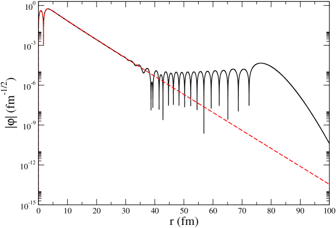
Figure 1: The modulus for the ⁶Li wave function in logarithmic scale obtained with the variational (black) and the Numerov’s (red dashed) methods using the $V_{H}$ potential.

In Fig. 1 we show a comparison for the ⁶Li reduced radial wave functions obtained, using the $V_{H}$ potential, with the Numerov’s or variational method. Similar results can be found for the other potentials. As it can be seen by inspection of the figure, the variational method is unable to reproduce the ⁶Li wave function at large distances, of the order of 30-40 fm. In this case the reduced wave function has been cured in order to get the correct asymptotic behaviour. Within the Numerov’s method, the long range wave function is constructed by hand. The agreement between the two methods is much nicer for the scattering problem, although the Numerov’s method has been used for the single channels. In these cases, the agreement between the two methods is at the order of 0.1%.

II.1.3 The ⁶Li nucleus and the $\alpha+d$ scattering state

The ⁶Li static properties, i.e. the binding energy respect to the $\alpha+d$ threshold, the $S$-state ANC, the magnetic dipole moment $\mu_{6}$ and the electric quadrupole moment $Q_{6}$ are given in Table 3. By inspection of the table we can conclude that each potential nicely reproduces the experimental binding energy, while only $V_{T}$, $V_{M}$ and $V_{G}$ give good values for the ANC. Also, the $V_{D}$ and $V_{G}$ potentials are the only ones which include the $D$-state contributions in the ⁶Li wave function. Therefore, the values of $\mu_{6}$ and $Q_{6}$ obtained with these potentials are closer to the experimental values, while $\mu_{6}$ and $Q_{6}$ calculated with the $V_{H}$, $V_{T}$, and $V_{M}$ potentials are simply those of the deuterium. Finally, we show in Fig. 2 the ⁶Li reduced wave function evaluated with each potential. The differences between the various potentials are quite pronounced for $r\leq 6$ fm. However, this is not too relevant for our reaction, which is peripheral and therefore most sensitive to the tail of the wave function and to the $S$-state ANC.

	$V_{H}$	$V_{T}$	$V_{M}$	$V_{D}$	$V_{G}$	EXP.
$B$	1.474	1.475	1.474	1.4735	1.4735	1.474
$C_{0}$	2.70	2.31	2.30	2.50	2.30	2.30
$\mu_{6}$	0.857	0.857	0.857	0.848	0.848	0.822
$Q_{6}$	0.286	0.286	0.286	-0.066	-0.051	-0.082

Table 3: The ⁶Li binding energy ($B$) in MeV, $S$-state ANC ($C_{0}$) in fm^1/2, magnetic dipole moment $\mu_{6}$ in $\mu_{N}$ and electric quadrupole moment $Q_{6}$ in fm² are calculated with the five different potential models $V_{H}$, $V_{T}$, $V_{M}$, $V_{D}$, and $V_{G}$. The available experimental data are also shown.

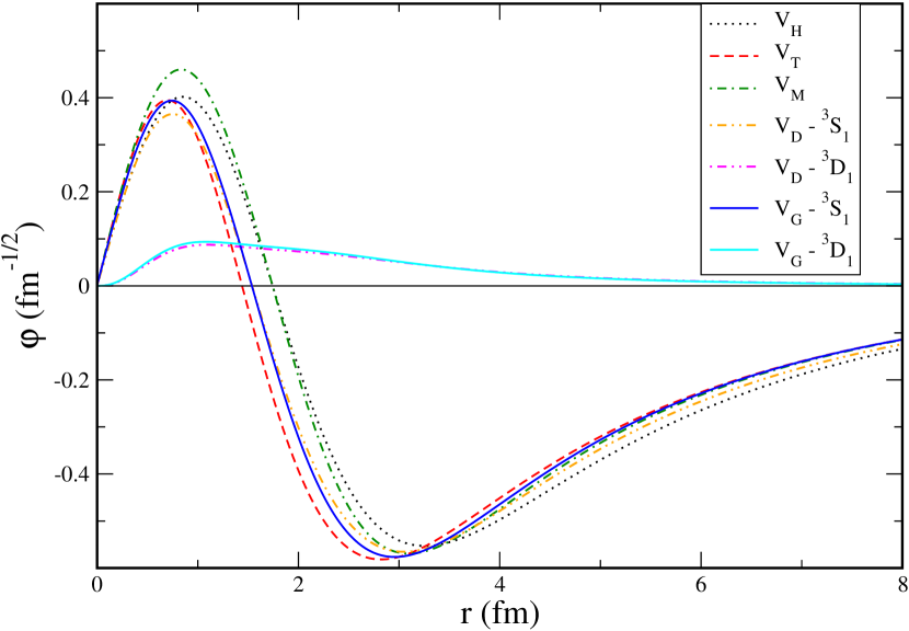
Figure 2: The ⁶Li reduced wave function evaluated with each potential model considered in this work.

For the initial $\alpha+d$ scattering state, the scattering phase shifts obtained with each potential are in good agreement with the experimental data, as it can be seen in Fig. 3 for the single channels and in Fig. 4 for the coupled channels. In particular, the results obtained with the $V_{H}$ ($V_{D}$) and $V_{M}$ ($V_{G}$) potentials coincide.

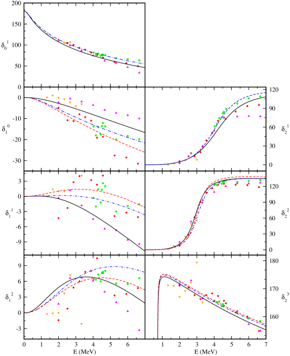
Figure 3: The phase shift $\delta_{\ell}^{J}$ for every partial wave ${}^{3}\ell_{J}$, where $\ell=\{0,~{}1,~{}2\}$. The data have been taken from Refs. jen83 ; mci67 ; gru75 ; bru82 ; kel70 . The phase shifts are given in degrees as a function of the center-of-mass relative energy in MeV. The shape of the experimental points indicates the article from which the data were taken: we use circles jen83 , triangles down mci67 , diamonds gru75 , squares bru82 and triangles up kel70 . The calculated phase shifts are obtained with the $V_{H}$ and $V_{M}$ (black solid line), $V_{T}$ (blue dash-dotted line), and $V_{D}$ and $V_{G}$ (red dashed line) potentials.

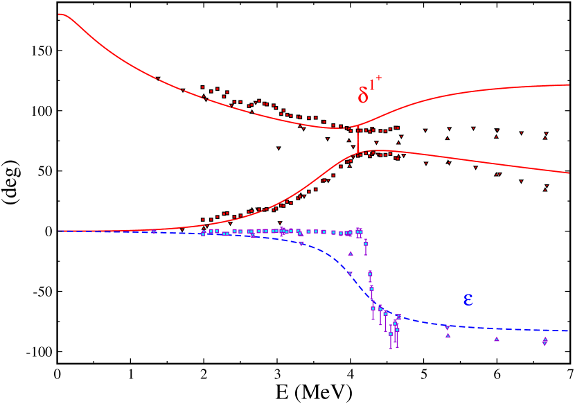
Figure 4: Same as Fig. 3, but for the coupled channels in the $J^{\pi}=1^{+}$ state. The phase shift results evaluated with the $V_{D}$ and the $V_{G}$ potentials for the coupled channels ${}^{3}S_{1}$ and ${}^{3}D_{1}$ are displayed with the two red solid lines, the results for the mixing angle $\varepsilon$ are displayed with the blue dashed line.

II.2 The transition operator

To evaluate the reaction cross section, we need to write down the nuclear electromagnetic current operator $\mathbf{J}^{\dagger}(\mathbf{q})$ of Eq. (4). This can be written as

$$\mathbf{J}^{\dagger}(\mathbf{q})=\int\mathrm{d}\mathbf{x}~{}\mathrm{e}^{i\mathbf{q}\mathbf{x}}~{}\mathbf{J}(\mathbf{x})$$ (32)

with

$$\mathbf{J}(\mathbf{x})=\sum_{i}~{}q_{i}\,\frac{\mathbf{p}_{i}}{m_{i}}~{}\delta^{3}(\mathbf{x}-\mathbf{x}_{i})\>,$$ (33)

where $\mathbf{p}_{i}$, $m_{i}$, $\mathbf{x}_{i}$ and $q_{i}$ are respectively the momentum, the mass, the position and the charge of the i-th particle. The matrix element appearing in Eq. (4), $\hat{\mathbf{\epsilon}}^{\dagger\lambda}_{\mathbf{q}}\cdot\left<\Psi_{{}^{6}{\rm Li}}(M)|\mathbf{J}^{\dagger}(\mathbf{q})|\Psi_{\alpha d}(M_{i})\right>$, can be rewritten expressing $\Psi_{{}^{6}{\rm Li}}(M)$ and $\Psi_{\alpha d}(M_{i})$ as

$$\Psi_{{}^{6}{\rm Li}}(M) = \frac{\varphi_{0}(r)}{r}Y_{00}(\theta,\phi)\chi_{1M}+\frac{\varphi_{2}(r)}{r}\sum_{m\sigma}\left<2m,1\sigma|1M\right>Y_{2m}(\theta,\phi)\chi_{1\sigma}$$ (34)

$$\Psi_{\alpha d}(M_{i}) = \sum_{\ell_{i}J_{i}}\>i^{\ell}\sqrt{4\pi(2\ell_{i}+1)}\left<\ell_{i}0,1M_{i}|J_{i}M_{i}\right>\>$$ (35)

$$\times \frac{\varphi_{\alpha+d}^{\ell_{i}J_{i}}(r)}{kr}\sum_{m^{\prime}\sigma^{\prime}}\left<\ell_{i}m^{\prime},1\sigma^{\prime}|J_{i}M_{i}\right>Y_{\ell_{i}m^{\prime}}(\theta,\phi)\chi_{1\sigma^{\prime}}\>,$$

where $\varphi_{\ell_{f}}(r)$ and $\varphi_{\alpha+d}^{\ell_{i}J_{i}}(r)$ are the ⁶Li and $\alpha+d$ reduced radial functions discussed in Sec. II.1. In the partial wave decomposition of Eq. (35), we have retained all the contributions up to $\ell_{i}=2$. By then performing a multipole expansion of the $\mathbf{J}^{\dagger}(\mathbf{q})$ operator, we obtain

$$\mathbf{\hat{\epsilon}}_{\mathbf{q}}^{\dagger\lambda}\cdot\mathbf{J}^{\dagger}(\mathbf{q})=-\sqrt{2\pi}\>\sum_{\Lambda\geq 1}(-i)^{\Lambda}\sqrt{2\Lambda+1}\left[E_{\Lambda\lambda}(q)+\lambda M_{\Lambda\lambda}(q)\right]\>,$$ (36)

where $\Lambda$ is the multipole index, while $E_{\Lambda\lambda}(q)$ and $M_{\Lambda\lambda}(q)$ are the so-called electric and magnetic multipoles of order $\Lambda$. They are defined as

$$E_{\Lambda\lambda}(q) = \frac{1}{q}\int\mathrm{d}\mathbf{x}\>[\nabla\times(j_{\Lambda}(qx)\mathbf{Y}^{\lambda}_{\Lambda\Lambda 1}(\mathbf{\hat{x}}))]\cdot\mathbf{J}(\mathbf{x})\>,$$ (37)

$$M_{\Lambda\lambda}(q) = \int\mathrm{d}\mathbf{x}\>j_{\Lambda}(qx)\mathbf{Y}^{\lambda}_{\Lambda\Lambda 1}(\mathbf{\hat{x}})\cdot\mathbf{J}(\mathbf{x})\>,$$ (38)

where $j_{\Lambda}(qx)$ is the spherical Bessel function of order $\Lambda$ and $\mathbf{Y}^{\lambda}_{\Lambda\Lambda 1}(\mathbf{\hat{x}})$ is the vector spherical harmonic of order $\Lambda$.

In this work we adopt the so-called long wavelength approximation (LWA), since, for the energy range of interest, the momentum of the emitted photon is much smaller than the ⁶Li dimension. This means that we can expand the multipoles in powers of $qr$. Furthermore, in the present calculation, we include only electric dipole and quadrupole multipoles, since it has been shown in Ref. nol01 that the magnetic multipoles are expected to give small contributions to the $S$-factor.

With this approximation, $E_{\Lambda\lambda}(q)$ can be written as

$$E_{\Lambda\lambda}(q)=Z_{e}^{(\Lambda)}\>\sqrt{\frac{\Lambda+1}{\Lambda}}f_{\Lambda}(qr)Y_{\Lambda\lambda}(\mathbf{\hat{x}})\>,$$ (39)

where muk16

$$f_{1}(x) = 3\frac{[(x^{2}-2)\sin x+2x\cos x]}{x^{2}}\>,$$ (40)

$$f_{2}(x) = 15\frac{[(5x^{2}-12)\sin x+(12-x^{2})x\cos x]}{x^{3}}\>,$$ (41)

and $Z_{e}^{(\Lambda)}$ is the so-called effective charge, and is given by

$$Z_{e}^{(\Lambda)}\equiv~{}Z_{d}\left(\frac{m_{\alpha}}{m_{\alpha}+m_{d}}\right)^{\Lambda}+Z_{\alpha}\left(-\frac{m_{d}}{m_{\alpha}+m_{d}}\right)^{\Lambda}\>.$$ (42)

Note that when only the first order contribution in the LWA is retained, $f_{\Lambda}(x)$ reduces to

$$f_{\Lambda}(x)=x^{\Lambda}\>.$$ (43)

The use of Eqs. (40) and (41) instead of Eq. (43) leads to an increase in the $S$-factor of the order of 1 %. This has been shown in Ref. muk16 and has been confirmed in the present work.

In the formalism of the LWA the total cross section of Eq. (3) can be written as

$$\sigma(E)=\sum_{\ell_{i}J_{i}\Lambda}~{}\sigma_{\ell_{i}J_{i}}^{(\Lambda)}(E)\>,$$ (44)

where $\sigma_{\ell_{i}J_{i}}^{(\Lambda)}(E)$ is the cross section evaluated with the electric $\Lambda$-multipole and the initial $\alpha+d$ state with orbital (total) angular momentum $\ell$ ($J_{i}$). It can be written as

$$\sigma_{\ell_{i}J_{i}}^{(\Lambda)}(E)\,=\,\frac{8\pi\>\alpha}{v_{\mathrm{rel}}\,k^{2}}\frac{q}{1+q/m_{6}}\,\,\frac{Z_{e}^{(\Lambda)\,2}}{[(2\Lambda+1)!!]^{2}}\frac{(\Lambda+1)(2\Lambda+1)}{\Lambda}(2\ell_{i}+1)(2J_{i}+1)\\ \times\bigg{[}\sum_{\ell_{f}}~{}(-)^{\ell_{f}}\sqrt{2\ell_{f}+1}\begin{pmatrix}\ell_{f}&\Lambda&\ell_{i}\\ 0&0&0\end{pmatrix}\begin{Bmatrix}J_{i}&\ell_{i}&1\\ \ell_{f}&J_{f}&\Lambda\end{Bmatrix}\,\>\int\>\mathrm{d}r\>\varphi_{{}^{6}{\rm Li}}^{\ell_{f}}(r)\>f_{\Lambda}(qr)\>\varphi_{\alpha+d}^{\ell_{i}J_{i}}(r)\bigg{]}^{2}\>.$$ (45)

For simplicity we define the partial $S$-factor as

$$S^{(\Lambda)}_{\ell_{i}J_{i}}(E)=E\>\sigma^{(\Lambda)}_{\ell_{i}J_{i}}(E)\>\exp{\left(2\pi\eta\right)}\>.$$ (46)

The results for these quantities evaluated with the $V_{G}$ potential are shown in Fig. 5. The ones for the other potentials have the same shapes and properties. The only difference comes for $V_{H}$ , $V_{T}$ and $V_{M}$ , where the contribution to the $S$-factor for the $\ell_{i}=0$ initial state are zero, being the transition ${}^{3}S_{1}\rightarrow{{}^{3}}S_{1}$ forbidden for each multipole term. Due to the nature of the LWA, the largest contribution to the total cross section, and therefore to the astrophysical $S$-factor, should be given by the $E_{1}$ transition, but, as we can see from Fig. 5, the $E_{1}$ transition dominates only at energies of the order of few keV. This is due to the so-called $E_{1}$ isotopic suppression. As we have seen the multipole expansion at $\Lambda$-th order for the electric terms depends on the square of the effective charge $Z_{e}^{(\Lambda)}$ and, for our reaction, $[Z_{e}^{(1)}]^{2}\simeq 1.6\times 10^{-5}$ and $[Z_{e}^{(2)}]^{2}\simeq 0.44$. Therefore the $E_{1}$ contribution to the $S$-factor is strongly suppressed, except for very low energies, where the other multipoles are reduced due to their energy dependence.

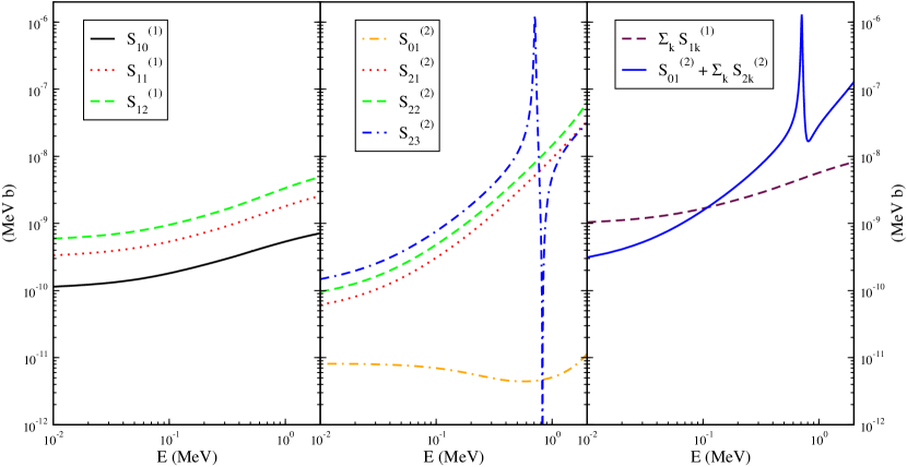
Figure 5: The partial astrophysical $S$-factors $S^{(\Lambda)}_{\ell_{i}J_{i}}(E)$, as defined in Eq. (46). On the left (central) panel the separate contribution for the dipole (quadrupole) transition are shown. The shape and color of the lines indicate the initial angular momentum. The red dotted and orange dash-dotted lines are used to indicate the transitions with $\ell_{i}=0$ and $\ell_{i}=2$, respectively, for $J_{i}=1$. For $J_{i}=0$, $J_{i}=2$, and $J_{i}=3$ solid black, green dashed and blue dot-dashed-dashed lines are used, respectively. On the right panel the total contribution for the dipole (quadrupole) is shown with a maroon dashed (blue solid) line.

II.3 The theoretical astrophysical $S$-factor

The calculated astrophysical $S$-factor is compared in Fig. 6 with the available experimental data from Refs. rob81 ; kie91 ; moh94 ; cec96 ; iga00 ; and14 ; tre17 . By inspection of the figure we can conclude that the tail of the $S$-factor at low energies has a strong dependence with respect to the ANC value. In fact, the three potentials which reproduce the ANC give very close results. The $V_{H}$ and $V_{D}$ potentials, giving a larger value for the ANC than the other potentials, predict higher values for the $S$-factor. Thanks to the relatively large number of considered potentials, we can give a rough estimate of the theoretical uncertainty of our predictions. Therefore, in Fig. 7 we show the same results of Fig. 6 as two bands, one obtained using all the five potentials and a much narrower one calculated with only the three potentials which reproduce the correct ANC value. As we can see from the figure, the theoretical uncertainty for the $S$-factor is much smaller in this second case: at center-of-mass energies $E\simeq 10$ keV, it is of the order of 2%, but it becomes at the 1% level at the LUNA available energies, i.e. for $E\simeq 100$ keV. On the other hand, if we consider all of the potentials, the previous estimates grow to 25% and 24% at $E\simeq 10$ and 100 keV, respectively. The available experimental data, though, are not accurate enough in order to discriminate between the results obtained with these five potentials. Therefore, in the following Section, where the primordial ⁶Li abundance is discussed, we consider conservatively the results for the astrophysical $S$-factor obtained with all the five potentials.

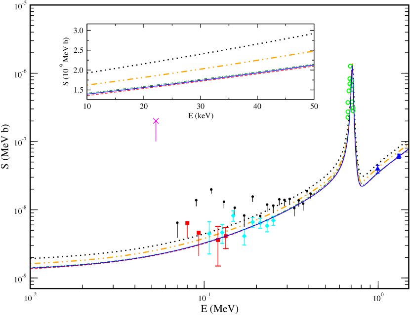
Figure 6: The total astrophysical $S$-factor evaluated with the five potential models considered in this work is compared with the data of Ref. rob81 (blue triangles), Ref. kie91 (black circles), Ref. moh94 (green circles), Ref. cec96 (magenta X), Ref. iga00 (cyan diamonds) and Ref. and14 ; tre17 (red squares). The data from Refs. kie91 ; cec96 are upper limits to the $S$-factor. In the insert, the tail of the $S$-factor in the energy range 10-50 keV. The dotted (black), dashed (red), dot-dashed (green), dot-dot-dashed (orange) and solid (blue) lines correspond to the results obtained with the $V_{H}$, $V_{T}$, $V_{M}$, $V_{D}$ and $V_{G}$ potentials, respectively.

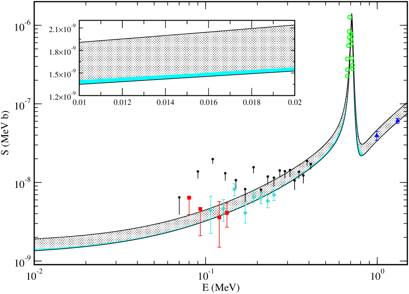
Figure 7: Same as Fig. 6 but with the theoretical results shown as a band. The (gray) dotted band is obtained using all the five potentials considered in this work, while the narrower (cyan) full band is obtained using only those three potentials ($V_{T}$ , $V_{M}$ , and $V_{G}$ ) which reproduce the experimental ANC value.

III The ⁶Li primordial abundance

⁶Li is expected to be produced during BBN with a rather low number density, ⁶Li/H $\sim 10^{-14}$, for the baryon density as obtained by the 2015 Planck results Ade:2015xua . This result still holds using the $S$-factor described in the previous Section (see below), and it is too small to be detectable at present. Actually, some positive measurements in old halo stars at the level of ⁶Li/⁷Li $\simeq 0.05$ were obtained in the last decade asp06 , but they may reflect the post-primordial production of this nuclide in Cosmic Ray spallation nucleosynthesis. Moreover, as we mentioned already, a more precise treatment of stellar atmosphere, including convection, shows that stellar convective motions can generate asymmetries in the line shape that mimic the presence of ⁶Li, so that the value 0.05 should be rather understood as a robust upper limit on ⁶Li primordial abundance. This does not mean that the issue is irrelevant for BBN studies since the study of the chemical evolution of the fragile isotopes of Li, Be and B could constraint the ⁷Li primordial abundance, and clarify the observational situation of Spite Plateau, see e.g. Ref. Olive:2016xmw .

The whole ⁶Li is basically produced via the $\alpha+d$ process, which is thus the leading reaction affecting the final yield of this isotope. The new theoretical $S$-factors detailed so far have been used to compute the thermal rate in the BBN temperature range, by folding the cross section with the Maxwell-Boltzmann distribution of involved nuclides. We have then changed the PArthENoPE code Pisanti:2007hk accordingly, and analyzed the effect of each different $S$-factor on the final abundance of ⁶Li, as function of the baryon density. For comparison, we also consider the value of the $S$-factor as obtained from fitting experimental data from Refs. RO81 ; MO94 ; IG00 ; AN14

$$S(E) = 10^{-9}\left(3.19368+6.94243\,E+32.204\,E^{2}\right)$$ (47)

$$+ \frac{9.96936\times 10^{-7}}{1.+4800.46\,(E-0.694061)^{2}}\ ,$$

as well as the NACRE 1999 fit nacre99 , which is used as benchmark rate in PArthENoPE public code. The results are shown in Fig. 8, normalized to NACRE 1999.

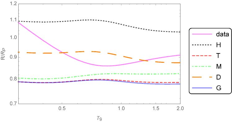
Figure 8: Rates vs. the temperature $T$ in units of $10^{9}$ K ($T_{9}$), corresponding to the astrophysical $S$-factors of the data fit (solid/magenta), and of the theoretical calculations with the five potentials used in this work (dotted/black, dashed/red, dot-dashed/green, long-dashed/orange and solid/blue, corresponding to $V_{H}$, $V_{T}$, $V_{M}$, $V_{D}$ and $V_{G}$ potentials, respectively), normalized to the standard rate used in PArthENoPE (NACRE 1999).

As we can see, the change is in the 10-20 % range. If we adopt the Planck 2015 best fit for the baryon density parameter $\Omega_{b}h^{2}=0.00226$ Ade:2015xua , we obtain values for the ⁶Li/H density ratio in the range $(0.9-1.4)\times 10^{-14}$, slightly smaller than what would be the result if the experimental data fit is used, as it can be seen in Table 4.

	bench	data	H	T	M	D	G
6Li/H $\times 10^{14}$	$1.1$	$1.7$	$1.4$	$1.1$	$1.1$	$1.0$	$0.93$

Table 4: Values of the final yield of ⁶Li (relative to H) for the five potential models considered in this paper, as well as for the NACRE 1999 rate, used as benchmark in PArthENoPE (bench) and using a fit of experimental data (data).

Notice that, at least with present sensitivity on ⁶Li yields, the dependence on the baryon density, or equivalently, the baryon to photon density ratio $\eta_{10}\sim 273.49\,\Omega_{b}h^{2}$, is quite mild, as shown in Fig. 9. The lower band in this plot cover the range of values obtained when the five potential models are used, and we can conservatively say that standard BBN predicts ⁶Li/H$=(0.9-1.8)\times 10^{-14}$. This range is also in good agreement with the results of other studies ham10 ; Cyburt:2015mya . In Fig. 9 we also show the final abundance of ⁷Be+⁷Li (upper band), which remains in the range $(4.2-4.7)\times 10^{-10}$, and it is, as expected, almost independent of the potential model adopted for the $\alpha+d$ radiative capture reaction considered here.

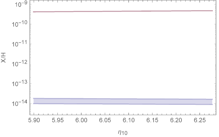
Figure 9: The X/H abundance for X=⁶Li (lower band) and X= ⁷Be+⁷Li (upper band). The theoretical uncertainty arising from the use of the five potential models considered in this paper is shown as a band.

IV Conclusions

The $\alpha+d$ radiative capture has been studied within a two-body framework, where the $\alpha$ particle and the deuteron are considered as structureless constituent of ⁶Li. The long-wavelength approximation (LWA) has been used, and the electric $E_{1}$ and $E_{2}$ multipoles have been retained. In order to study the accuracy that the present theoretical framework can reach, we have used five different models for the $\alpha+d$ interaction, among which also, for the first time, potential models with a tensor term, able to reproduce the magnetic dipole and electric quadrupole moments of ⁶Li , as well the $S$-state ANC and the $\alpha+d$ scattering phase shifts. The theoretical uncertainty to the astrophysical $S$-factor, the observable of interest, is of the order of $\sim$ 20% if all the five potential models are retained, but reduces to few % if only those potentials which reproduce the $S$-state ANC are considered. The experimental data, however, are affectd by an uncertainty much larger than the theoretical one.

The calculated values for the $\alpha+d$ astrophysical $S$-factor have been used in the PArthENoPE public code in order to estimate the ⁶Li and ⁷Li+⁷Be primordial abundances. The ⁶Li abundance is predicted to be slightly smaller than what would result from the available experimental data and from the NACRE 1999 compilation, but still in the range of $(0.9-1.8)\times 10^{-14}$. We conclude that this result of standard BBN is thus quite robust. Further studies about ⁶Li astrophysical measurement may be needed to check the claim of a much larger ratio ⁶Li/⁷Li obtained in Ref. asp06 . On the other hand, the final ⁷Li+⁷Be abundance is almost independent on the result for the astrophysical $S$-factor presented here, and is found to be in the range of $(4.2-4.7)\times 10^{-10}$.

Finally, we would like to notice that the present calculation for the astrophysical $S$-factor is, to our knowledge, the most up-to-date one working within a two-body framework. However, the assumption that the deuteron is a structureless constituent of ⁶Li can be considered rather weak, and the present study could be improved if the six-body systems are viewed as a core of an $\alpha$ particle and two nucleons, i.e. as a three-body systems. The first steps within this three-body framework have been done in Ref. Tur16 , and further work along this line is currently underway.

References

- (1) M. Asplund, D. Lambert, P.E. Nissen, F. Primas, and V. Smith, Astrophys. J. 644, 229 (2006).
- (2) R. Cayrel et al., Astron. Astrophys. 473, L37 (2007).
- (3) A.E.G. Perez, W. Aoki, S. Inoue, S.G. Ryan, T.K. Suzuki, and M. Chiba, Astron. Astrophys. 504, 213 (2009).
- (4) M. Steffen, R. Cayrel, P. Bonifacio, H.G. Ludwig, and E. Caffau, IAU Symposium 265, 23 (2010).
- (5) K. Lind, J. Melendez, M. Asplund, R. Collet, and Z. Magic, Astron. Astrophys. 544, A96 (2013).
- (6) R.G.H. Robertson, P. Dyer, R.A. Warner, R.C. Melin, T.J. Bowles, A.B. McDonald, G.C. Ball, W.G. Davies, and E.D. Earle, Phys. Rev. Lett. 47, 1867 (1981)
- (7) J. Kiener, H.J. Gils, H. Rebel, S. Zagromski, G. Gsottschneider, N. Heide, H. Jelitto, J. Wentz, and G. Baur, Phys. Rev. C 44, 2195 (1991)
- (8) P. Mohr, V. Kölle, S. Wilmes, U. Atzrott, G. Staudt, J.W. Hammer, H. Krauss, and H. Oberhummer, Phys. Rev. C 50, 1543 (1994)
- (9) F.E. Cecil, J. Yan, and C.S. Galovich, Phys. Rev. C 53, 1967 (1996)
- (10) S.B. Igamov and R. Yarmukhamedov, Nucl. Phys. A 673, 509 (2000)
- (11) M. Anders et al., Phys. Rev. Lett. 113, 042501 (2014)
- (12) D. Trezzi et al., Astroparticle Physics 89, 57 (2017).
- (13) K. M. Nollett, R. B. Wiringa, R. Schiavilla, Phys. Rev. C 63, 024003 (2001).
- (14) F. Hammache et al., Phys. Rev. C 82, 065803 (2010)
- (15) E.M. Tursunov, S.A. Turakulov, and P. Descouvemont, Phys. Atom. Nucl. 78, 193 (2015)
- (16) A.M. Mukhamedzhanov, L.D. Blokhintsev, and B.F. Irgaziev, Phys. Rev. C 83, 055805 (2011)
- (17) S.B. Dubovichenko, Phys. Atom. Nucl. 61, 162 (1998)
- (18) S. B. Dubovichenko and A. V. Dzhazairov-Kakhramanov, Phys. Atom. Nucl. 57, 733 (1994).
- (19) B. Jenny, W. Grüebler, V. König, P. A. Schmelzbach, and C. Schweizer, Nucl. Phys. A 397, 61 (1983).
- (20) L. C. McIntyre and W. Haeberli, Nucl. Phys. A 91, 382 (1967).
- (21) W. Grübler, P. A. Schmelzbach, V. König, P. Risler, and D. Boerma, Nucl. Phys. A 242, 265 (1975).
- (22) M. Bruno, F. Cannata, M. D’Agostino, C. Maroni, I. Massa, and M. Lombardi, Nuovo Cimento A 68, 35 (1982).
- (23) L. G. Keller and W. Haeberli, Nucl. Phys. A 156, 465 (1970).
- (24) L.E. Marcucci, M. Piarulli, M. Viviani, L. Girlanda, A. Kievsky, S. Rosati, R. Schiavilla, Phys. Rev. C 83, 014002 (2011).
- (25) A.M. Mukhamedzhanov, Shubhchintak, and C.A. Bertulani, Phys. Rev. C 93, 045805 (2016)
- (26) P.A.R. Ade et al. [Planck Collaboration], Astron. Astrophys. 594, A13 (2016)
- (27) C. Patrignani et al. [Particle Data Group], Chin. Phys. C 40, no. 10, 100001 (2016).
- (28) O. Pisanti, A. Cirillo, S. Esposito, F. Iocco, G. Mangano, G. Miele, and P.D. Serpico, Comput. Phys. Commun. 178, 956 (2008)
- (29) R.G.H. Robertson et al., Phys. Rev. Lett. 47, 1867 (1981); Erratum: R.G.H. Robertson et al., Phys. Rev. Lett. 75, 4334 (1995).
- (30) P. Mohr, V. Kölle, S. Wilmes, U. Atzrott, G. Staudt, J.W. Hammer, H. Krauss, and H. Oberhummer, Phys. Rev. C 50, 1543 (1994).
- (31) S.B. Igamov and R. Yarmukhamedov, Nucl. Phys. A 673, 509 (2000).
- (32) M. Anders et al., Phys. Rev. Lett. 113, 042501 (2014).
- (33) C. Angulo et al., Nucl. Phys. A 656, 3 (1999).
- (34) R.H. Cyburt, B.D. Fields, K.A. Olive, and T.H. Yeh, Rev. Mod. Phys. 88, 015004 (2016).
- (35) E.M. Tursunov, A.S. Kadyrov, S.A. Turakulov, and I. Bray, Phys. Rev. C 94, 015801 (2016).