UMTG–291

The integrable quantum group invariant
$A_{2n-1}^{(2)}$ and $D_{n+1}^{(2)}$ open spin chains
Rafael I. Nepomechie , Rodrigo A. Pimenta , and Ana L. Retore

A family of $A_{2n}^{(2)}$ integrable open spin chains with $U_{q}(C_{n})$ symmetry was recently identified in arXiv:1702.01482. We identify here in a similar way a family of $A_{2n-1}^{(2)}$ integrable open spin chains with $U_{q}(D_{n})$ symmetry, and two families of $D_{n+1}^{(2)}$ integrable open spin chains with $U_{q}(B_{n})$ symmetry. We discuss the consequences of these symmetries for the degeneracies and multiplicities of the spectrum. We propose Bethe ansatz solutions for two of these models, whose completeness we check numerically for small values of $n$ and chain length $N$. We find formulas for the Dynkin labels in terms of the numbers of Bethe roots of each type, which are useful for determining the corresponding degeneracies. In an appendix, we briefly consider $D_{n+1}^{(2)}$ chains with other integrable boundary conditions, which do not have quantum group symmetry.

1 Introduction

Quantum spin chains are quantum many-body systems that have applications in diverse fields, ranging from statistical mechanics [1, 2], condensed-matter theory [3, 4] and quantum information theory [5] to quantum field theory and string theory [6]. The simplest anisotropic spin chains are arguably those that are integrable and have quantum group [7] symmetry. Indeed, integrability allows access to the spectrum, and quantum group symmetry can account for the degeneracies and multiplicities. The prototypical example is the $U_{q}(A_{1})$-invariant open spin-1/2 chain [8], whose integrability follows from [9, 10].

Generalizations of this example can be constructed systematically. Integrable bulk interactions are encoded in solutions of the Yang-Baxter equation, which in this context are called R-matrices. Infinite families of anisotropic R-matrices associated with corresponding affine Lie algebras were found in [11, 12, 13, 14]. Similarly, integrable boundary conditions are encoded in solutions of the boundary Yang-Baxter equation (BYBE) [10, 15, 16], which in this context are called $K^{\mp}$-matrices. Quantum group symmetry can be realized by choosing these $K^{\mp}$-matrices appropriately.

Several infinite families of integrable open spin chains that are quantum group invariant were identified in [17]. Bethe ansatz solutions of these models were found in [18, 19, 20, 21, 22]. The integrable quantum-group-invariant spin chains identified in [17] are all constructed using the R-matrices in [13, 14] together with the simplest $K^{-}$-matrix, namely, the identity matrix. For example, the integrable spin chain constructed with the $A_{2n}^{(2)}$ R-matrix and $K^{-}=\mathbb{I}$ has $U_{q}(B_{n})$ symmetry. The appearance of $B_{n}$ can be understood from the fact (see e.g. [23]) that it is the subalgebra of $A_{2n}$ that remains invariant under the order-2 diagram automorphism.

It was recently observed that the integrable spin chain constructed with the $A_{2n}^{(2)}$ R-matrix and with a different choice of $K^{-}$ [17, 24, 25] has instead $U_{q}(C_{n})$ symmetry [26]. (The case $n=1$, corresponding to the Izergin-Korepin R-matrix [27], was analyzed in [28].) The appearance of $C_{n}$ can be inferred from the extended Dynkin diagram for $A_{2n}^{(2)}$ shown in Fig. 1: removing the leftmost node yields the Dynkin diagram for the subalgebra $C_{n}$ shown in Fig 2. (Removing the rightmost node yields the Dynkin diagram for the subalgebra $B_{n}$; and indeed the spin chain with $K^{-}=\mathbb{I}$ has $U_{q}(B_{n})$ symmetry, as already noted above.)

(a)

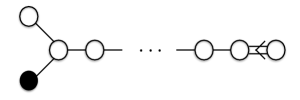
(b)

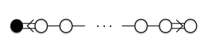
(c)

Figure 1: Extended Dynkin diagrams for (a) $A^{(2)}_{2n}$ (b) $A^{(2)}_{2n-1}$ (c) $D^{(2)}_{n+1}$

This observation in [26] opens the door to (at least) doubling the list of integrable quantum-group-invariant spin chains identified in [17]: starting with an R-matrix corresponding to a given affine Lie algebra, it should be possible to construct a different integrable spin chain that is invariant under the quantum group dictated by the corresponding extended Dynkin diagram (as illustrated above) by finding an appropriate $K^{-}\neq\mathbb{I}$.

We carry out here the above program for the R-matrices corresponding to the two remaining infinite families of twisted affine Lie algebras, namely $A_{2n-1}^{(2)}$ and $D_{n+1}^{(2)}$. For $A_{2n-1}^{(2)}$ with $n>1$, we expect to find a new integrable spin chain with $U_{q}(D_{n})$ symmetry, since removing the rightmost node of the extended Dynkin diagram (see again Fig. 1) yields the Dynkin diagram for the subalgebra $D_{n}$. (Removing one of the two leftmost nodes yields the Dynkin diagram for the subalgebra $C_{n}$, and indeed the spin chain with $K^{-}=\mathbb{I}$ has $U_{q}(C_{n})$ symmetry [17].)

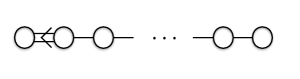
(a)

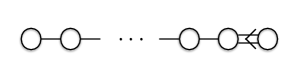
(b)

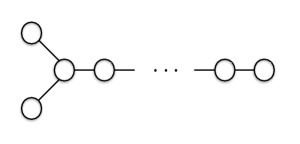
(c)

Figure 2: Dynkin diagrams for (a) $B_{n}$ (b) $C_{n}$ (c) $D_{n}$

Integrable quantum-group-invariant spin chains with the $D_{n+1}^{(2)}$ R-matrix were not constructed in [17], since the corresponding BYBE does not have the solution $K^{-}=\mathbb{I}$. However, several solutions of this BYBE were found in [29]. We show here that two of these solutions can be used to construct integrable spin chains with $U_{q}(B_{n})$ symmetry, as expected from the extended Dynkin diagram for $D_{n+1}^{(2)}$ (see again Fig. 1), since removing either the leftmost or rightmost node yields the Dynkin diagram for the subalgebra $B_{n}$.

The outline of this paper is as follows. In Sec. 2 we recall basic properties of the $A_{2n-1}^{(2)}$ and $D_{n+1}^{(2)}$ R-matrices, whose explicit expressions are given in Appendix A. In Sec. 3 we introduce a pair of K-matrices for each R-matrix, which in a subsequent section will be shown to lead to quantum group symmetry. We briefly review in Sec. 4 how the R-matrices and K-matrices can be used to construct the transfer matrix, and consequently the Hamiltonian, of an integrable open spin chain. We then use an identity (4.8) to show that – for each of our four choices of K-matrices – the corresponding Hamiltonians can be expressed essentially as sums of two-body terms, see (4.9), (4.16), (4.23) and (4.27). We use this fact in Sec. 5 to show that each of these four Hamiltonians has quantum group symmetry. We also discuss the consequences of these symmetries for the degeneracies and multiplicities of the spectrum. In Secs. 6 and 7 we present Bethe ansatz solutions for all but one of these models, and numerically check their completeness. We also find formulas for the Dynkin labels in terms of the numbers of Bethe roots of each type, which are useful for determining the corresponding degeneracies. In Sec. 8 we briefly summarize our main results and note some remaining open problems. In Appendix B, we briefly consider $D_{n+1}^{(2)}$ chains with other integrable boundary conditions, which do not have quantum group symmetry.

2 R-matrices: generalities

The R-matrices for $A_{2n-1}^{(2)}$ and $D_{n+1}^{(2)}$ are given explicitly in Appendix A. These R-matrices map ${\cal V}\otimes{\cal V}$ to itself, where ${\cal V}$ is a $d$-dimensional vector space, where

$$d=\left\{\begin{array}[]{cc}2n&\mbox{ for }A_{2n-1}^{(2)}\\ 2n+2&\mbox{ for }D_{n+1}^{(2)}\end{array}\right.\,,$$ (2.1)

and satisfy the Yang-Baxter equation (YBE) on ${\cal V}\otimes{\cal V}\otimes{\cal V}$

$$R_{12}(u-v)\,R_{13}(u)\,R_{23}(v)=R_{23}(v)\,R_{13}(u)\,R_{12}(u-v)\,.$$ (2.2)

As usual, $R_{12}=R\otimes\mathbb{I}\,,R_{23}=\mathbb{I}\otimes R\,,R_{13}={\cal P}_{23}R_{12}{\cal P}_{23}$, where $\mathbb{I}$ is the identity matrix on ${\cal V}$, and ${\cal P}$ is the permutation matrix on ${\cal V}\otimes{\cal V}$

$${\cal P}=\sum_{\alpha,\beta=1}^{d}e_{\alpha\beta}\otimes e_{\beta\alpha}\,,$$ (2.3)

and $e_{\alpha\beta}$ are the $d\times d$ elementary matrices with elements $(e_{\alpha\beta})_{ij}=\delta_{\alpha,i}\delta_{\beta,j}$. In addition, these R-matrices have the following properties: $PT$ symmetry

$$R_{21}(u)\equiv{\cal P}_{12}\,R_{12}(u)\,{\cal P}_{12}=R_{12}^{t_{1}t_{2}}(u)\,,$$ (2.4)

unitarity

$$R_{12}(u)\ R_{21}(-u)=\zeta(u)\,\mathbb{I}\otimes\mathbb{I}\,,$$ (2.5)

where $\zeta(u)$ is given by

$$\zeta(u)=\xi(u)\,\xi(-u)\,,\qquad\xi(u)=\left\{\begin{array}[]{cc}-2\sinh(\frac{u}{2}+2\eta)\cosh(\frac{u}{2}+2n\eta)&\mbox{ for }A_{2n-1}^{(2)}\\ 4\sinh(u+2\eta)\sinh(u+2n\eta)&\mbox{ for }D_{n+1}^{(2)}\end{array}\right.\,,$$ (2.6)

regularity

$$R(0)=\xi(0)\,{\cal P}\,,$$ (2.7)

and crossing symmetry

$$R_{12}(u)=V_{1}\,R_{12}^{t_{2}}(-u-\rho)\,V_{1}=V_{2}^{t_{2}}\,R_{12}^{t_{1}}(-u-\rho)\,V_{2}^{t_{2}}\,,$$ (2.8)

where the crossing parameter $\rho$ is given by

$$\rho=\left\{\begin{array}[]{cc}-4n\eta-i\pi&\mbox{ for }A_{2n-1}^{(2)}\\ -2n\eta&\mbox{ for }D_{n+1}^{(2)}\end{array}\right.\,.$$ (2.9)

The crossing matrix $V$ is given by

$$V=\sum_{k=1}^{d}v_{k}\,e_{k,d+1-k}\,,$$ (2.10)

where

$$v_{k} =\left\{\begin{array}[]{cl}ie^{-2(n+1-k)\eta}&k=1,\ldots,n\\ -ie^{-2(n-k)\eta}&k=n+1,\ldots,2n\end{array}\right.\mbox{ for }A_{2n-1}^{(2)}$$ (2.13)

$$v_{k} =\left\{\begin{array}[]{cl}e^{-(2n+1-2k)\eta}&k=1,\ldots,n\\ 1&k=n+1,n+2\\ e^{-(2n+5-2k)\eta}&k=n+3,\ldots,2n+2\end{array}\right.\mbox{ for }D_{n+1}^{(2)}\,,$$ (2.17)

and satisfies $V^{2}=\mathbb{I}$. The corresponding matrix $M$ is defined by

$$M=\epsilon V^{t}\,V\,,\qquad\epsilon=\left\{\begin{array}[]{cc}-1&\mbox{ for }A_{2n-1}^{(2)}\\ +1&\mbox{ for }D_{n+1}^{(2)}\end{array}\right.\,,$$ (2.18)

and is given by a diagonal matrix

$$M=\left\{\begin{array}[]{ll}\mathop{\rm diag}\nolimits(e^{4(n+\frac{1}{2}-\bar{\alpha})\eta})\,,\qquad\alpha=1,2,\ldots\,,2n&\mbox{ for }A_{2n-1}^{(2)}\\ \mathop{\rm diag}\nolimits(e^{4(n+\frac{3}{2}-\bar{\alpha})\eta})\,,\qquad\alpha=1,2,\ldots\,,2n+2&\mbox{ for }D_{n+1}^{(2)}\end{array}\right.$$ (2.19)

where $\bar{\alpha}$ is defined by (A.5) for $A_{2n-1}^{(2)}$ and by (A.15) for $D_{n+1}^{(2)}$.

3 K-matrices

The matrix $K^{-}(u)$, which maps ${\cal V}$ to itself, is a solution of the so-called reflection equation or boundary Yang-Baxter equation (BYBE) on ${\cal V}\otimes{\cal V}$ [10, 15, 16]

$$R_{12}(u-v)\,K^{-}_{1}(u)\ R_{21}(u+v)\,K^{-}_{2}(v)=K^{-}_{2}(v)\,R_{12}(u+v)\,K^{-}_{1}(u)\,R_{21}(u-v)\,.$$ (3.1)

We assume that it has the regularity property

$$K^{-}(0)=\kappa\,\mathbb{I}\,.$$ (3.2)

For the corresponding $K^{+}$-matrix, we shall always take

$$K^{+}(u)=K^{-\,t}(-u-\rho)\,M\,,$$ (3.3)

where $M$ is defined by (2.18). For any solution $K^{-}(u)$ of the BYBE (3.1), the “isomorphism” (3.3) gives a solution of the corresponding BYBE for $K^{+}(u)$ [10, 30]

$$R_{12}(-u+v)\,K_{1}^{+\,t_{1}}(u)\,M^{-1}_{1}\,R_{21}(-u-v-2\rho)\,M_{1}\,K_{2}^{+\,t_{2}}(v)$$ (3.4)

$$\quad=K^{+\,t_{2}}_{2}(v)\,M_{1}\,R_{12}(-u-v-2\rho)\,M^{-1}_{1}\,K^{+\,t_{1}}_{1}(u)\,R_{21}(-u+v)\,.$$

3.1 $A_{2n-1}^{(2)}$ K-matrices

For the BYBE (3.1) with Kuniba’s $A_{2n-1}^{(2)}$ R-matrix (A.1)-(A.7), only two solutions have (to our knowledge) been reported [20, 24], both of which are diagonal. We have searched for additional diagonal solutions with $n\geq 2$, and we have found only one more:

$$K^{-}(u)=\mathop{\rm diag}\nolimits(\frac{e^{-u}+\beta}{e^{u}+\beta},1,1,\ldots,1,1,\frac{e^{u+4(n-1)\eta}-\beta}{e^{-u+4(n-1)\eta}-\beta})\,,$$ (3.5)

where $\beta$ is an arbitrary parameter. This solution reduces to the identity matrix $\mathbb{I}_{2n\times 2n}$ in the limit $\beta\rightarrow\infty$. We have not looked for non-diagonal solutions, which would require significantly more effort.

For $A_{2n-1}^{(2)}$, we shall henceforth consider the following two $2n\times 2n$ diagonal $K^{-}$-matrices, to which we refer by I and II:

$$A_{2n-1}^{(2)}-\text{I}: \qquad K^{-}(u)=\mathbb{I}_{2n\times 2n}\,,$$ (3.6)

$$A_{2n-1}^{(2)}-\text{II}: \qquad K^{-}(u)=\left(\begin{array}[]{cc}e^{-u}\,\mathbb{I}_{n\times n}&\\ &e^{u}\,\mathbb{I}_{n\times n}\end{array}\right)\,.$$ (3.9)

These two solutions of the $A_{2n-1}^{(2)}$ BYBE (3.1) were found in [17, 20] and [24], respectively. Both solutions evidently satisfy the regularity property (3.2) with

$$\kappa=1\,.$$ (3.10)

3.2 $D_{n+1}^{(2)}$ K-matrices

Several solutions of the BYBE (3.1) with the $D_{n+1}^{(2)}$ R-matrix (A.9) are known [29, 32]. A diagonal solution is given by the following $(2n+2)\times(2n+2)$ matrix [29]

$$K^{-}(u)=\left(\begin{array}[]{cccc}\mathbb{I}_{n\times n}&&&\\ &\mathsf{k}_{1}(u)&&\\ &&\mathsf{k}_{2}(u)&\\ &&&e^{2u}\,\mathbb{I}_{n\times n}\end{array}\right)\,,$$ (3.11)

where

$$\mathsf{k}_{1}(u)=\frac{e^{u}-ie^{-n\eta}}{e^{-u}-ie^{-n\eta}}\,,\qquad\mathsf{k}_{2}(u)=\frac{e^{u}+ie^{-n\eta}}{e^{-u}+ie^{-n\eta}}\,.$$ (3.12)

We consider this solution briefly in Appendix B.1.

Two block-diagonal solutions of the $D_{n+1}^{(2)}$ BYBE are also known : one of these solutions is given by the $(2n+2)\times(2n+2)$ matrix

$$K^{-}(u)=\left(\begin{array}[]{cccc}\mathsf{k}_{0}(u)\,\mathbb{I}_{n\times n}&&&\\ &\mathsf{k}_{1}(u)&\mathsf{k}_{2}(u)&\\ &\mathsf{k}_{3}(u)&\mathsf{k}_{4}(u)&\\ &&&\mathsf{k}_{5}(u)\,\mathbb{I}_{n\times n}\end{array}\right)\,,$$ (3.13)

where

$$\mathsf{k}_{0}(u) =(e^{2u}+e^{2n\eta})(\xi_{-}^{2}e^{u+2n\eta}-e^{-u})\,,$$

$$\mathsf{k}_{1}(u) =\frac{1}{2}(e^{2u}+1)\left[2\xi_{-}e^{2n\eta}(e^{2u}-1)-e^{u}(1-\xi_{-}^{2}e^{2n\eta})(1+e^{2n\eta})\right]\,,$$

$$\mathsf{k}_{2}(u) =\mathsf{k}_{3}(u)=\frac{1}{2}e^{u}(e^{2u}-1)(1+\xi_{-}^{2}e^{2n\eta})(1-e^{2n\eta})\,,$$

$$\mathsf{k}_{4}(u) =\frac{1}{2}(e^{2u}+1)\left[-2\xi_{-}e^{2n\eta}(e^{2u}-1)-e^{u}(1-\xi_{-}^{2}e^{2n\eta})(1+e^{2n\eta})\right]\,,$$

$$\mathsf{k}_{5}(u) =(e^{2u}+e^{2n\eta})(\xi_{-}^{2}e^{u+2n\eta}-e^{3u})\,,$$ (3.14)

and $\xi_{-}$ is an arbitrary boundary parameter. We consider this solution briefly in Appendix B.2. Another block-diagonal solution has the same matrix structure (3.13), but the matrix elements are instead given by

$$\mathsf{k}_{0}(u) =(e^{2u}-e^{2n\eta})(\xi_{-}^{2}e^{u}-e^{-u})\,,$$

$$\mathsf{k}_{1}(u) =\mathsf{k}_{4}(u)=\frac{1}{2}(e^{2u}+1)e^{u}(1-e^{2n\eta})(\xi_{-}^{2}-1)\,,$$

$$\mathsf{k}_{2}(u) =\frac{1}{2}(e^{2u}-1)\left[2e^{n\eta}(e^{2u}+1)\xi_{-}+e^{u}(1+e^{2n\eta})(1+\xi_{-}^{2})\right]\,,$$

$$\mathsf{k}_{3}(u) =\frac{1}{2}(e^{2u}-1)\left[-2e^{n\eta}(e^{2u}+1)\xi_{-}+e^{u}(1+e^{2n\eta})(1+\xi_{-}^{2})\right]\,,$$

$$\mathsf{k}_{5}(u) =(e^{2u}-e^{2n\eta})(\xi_{-}^{2}-e^{2u})e^{u}\,,$$ (3.15)

where $\xi_{-}$ is again an arbitrary boundary parameter.

For $\xi_{-}=0$, these block-diagonal solutions have the matrix structure

$$K^{-}(u)=-2e^{2u+n\eta}\left(\begin{array}[]{cccc}k_{-}(u)\,\mathbb{I}_{n\times n}&&&\\ &k_{1}(u)&k_{2}(u)&\\ &k_{2}(u)&k_{1}(u)&\\ &&&k_{+}(u)\,\mathbb{I}_{n\times n}\end{array}\right)\,,$$ (3.16)

and the matrix elements are given by

$$D_{n+1}^{(2)}-\text{I}: \qquad k_{\mp}(u)=e^{\mp 2u}\cosh(u-n\eta)\,,\quad k_{1}(u)=\cosh(u)\cosh(n\eta)\,,$$

$$\qquad\qquad k_{2}(u)=\sinh(u)\sinh(n\eta)\,,$$ (3.17)

$$D_{n+1}^{(2)}-\text{II}: \qquad k_{\mp}(u)=e^{\mp 2u}\sinh(u-n\eta)\,,\quad k_{1}(u)=-\cosh(u)\sinh(n\eta)\,,$$

$$\qquad\qquad k_{2}(u)=-\sinh(u)\cosh(n\eta)\,.$$ (3.18)

corresponding to (3.14) and (3.15), respectively. We shall henceforth focus primarily on the two solutions (3.17) and (3.18), to which we refer by I and II, respectively. These solutions satisfy the regularity property (3.2), with

$$\kappa=\left\{\begin{array}[]{cl}-2e^{n\eta}\,\cosh(n\eta)&\mbox{ for }D_{n+1}^{(2)}-\text{I}\\ 2e^{n\eta}\,\sinh(n\eta)&\mbox{ for }D_{n+1}^{(2)}-\text{II}\\ \end{array}\right.\,.$$ (3.19)

We observe that the $A_{2n-1}^{(2)}$ $K^{-}$-matrices (3.6)-(3.9) and the $D_{n+1}^{(2)}$ $K^{-}$-matrices (3.16) are symmetric

$$\left(K^{-}(u)\right)^{t}=K^{-}(u)\,.$$ (3.20)

4 Transfer matrix and Hamiltonian

The transfer matrix $t(u)$ for an integrable open quantum spin chain with $N$ sites, which acts on the quantum space ${\cal V}^{\otimes N}$, is given by [10]

$$t(u)=\mathop{\rm tr}\nolimits_{a}K^{+}_{a}(u)\,T_{a}(u)\,K^{-}_{a}(u)\,\hat{T}_{a}(u)\,,$$ (4.1)

where the monodromy matrices are defined by

$$T_{a}(u)=R_{aN}(u)\ R_{aN-1}(u)\ \cdots R_{a1}(u)\,,\qquad\hat{T}_{a}(u)=R_{1a}(u)\ \cdots R_{N-1a}(u)\ R_{Na}(u)\,,$$ (4.2)

and the trace in (4.1) is over the auxiliary space, which we denote by $a$. By construction, the transfer matrix satisfies the fundamental commutativity property [10]

$$\left[t(u)\,,t(v)\right]=0\hbox{ for all }u\,,v\,.$$ (4.3)

The transfer matrix also has crossing symmetry [18]

$$t(u)=t(-u-\rho)\,.$$ (4.4)

The corresponding integrable open-chain Hamiltonian is given (up to multiplicative and additive constants) by $t^{\prime}(0)$, which is local as a consequence of the regularity properties (2.7) and (3.2). After some computation, one finds (up to terms proportional to the identity) [10]

$${\cal H}\sim\sum_{k=1}^{N-1}h_{k,k+1}+\frac{1}{2\kappa}K^{-\,^{\prime}}_{1}(0)+\frac{1}{\mathop{\rm tr}\nolimits K^{+}(0)}\mathop{\rm tr}\nolimits_{0}K^{+}_{0}(0)h_{N0}\,,$$ (4.5)

where the two-site Hamiltonian $h_{k,k+1}$ is given by

$$h_{k,k+1}=\frac{1}{\xi(0)}{\cal P}_{k,k+1}R^{\prime}_{k,k+1}(0)\,.$$ (4.6)

We now proceed as in [26] to simplify the expression (4.5), which will be needed in the subsequent section for proving the quantum group invariance of the Hamiltonian. Such a simplification is possible due to the identity [26]

$$\mathop{\rm tr}\nolimits_{1}K^{-}_{1}(-u-\rho)\,M_{1}\,R_{12}(2u)\,{\cal P}_{12}=f(u)\,V_{2}\,K^{-\,t_{2}}_{2}(u)\,V_{2}\,,$$ (4.7)

where $f(u)$ is a scalar function. In view of the isomorphism (3.3) and the fact that the $K^{-}$-matrices are symmetric (3.20), this identity can be rewritten as

$$\mathop{\rm tr}\nolimits_{1}K^{+}_{1}(u)\,{\cal P}_{12}R_{21}(2u)=f(u)\,V_{2}\,K^{-}_{2}(u)\,V_{2}\,.$$ (4.8)

In order to go further, we must now consider the various cases separately.

4.1 $A_{2n-1}^{(2)}$ - case I

For the case $A_{2n-1}^{(2)}-\text{I}$ (3.6), it follows from (4.8) as in [26] that the third term in (4.5) is proportional to the identity, while the second term evidently vanishes. The Hamiltonian therefore reduces to a sum of two-site Hamiltonians [17]

$${\cal H}^{(A_{2n-1}^{(2)}-\text{I})}=\sum_{k=1}^{N-1}h_{k,k+1}\,.$$ (4.9)

It is related to the transfer matrix (4.1) by

$${\cal H}^{(A_{2n-1}^{(2)}-\text{I})}=\frac{1}{c_{1}}t^{\prime}(0)+c_{2}\mathbb{I}^{\otimes N}\,,$$ (4.10)

with

$$c_{1} =4^{N+1}\sinh(2n\eta)\,\cosh(2(n+1)\eta)\,\sinh^{2N-1}(2\eta)\,\cosh^{2N}(2n\eta)\,,$$

$$c_{2} =\frac{\cosh(2(3n+1)\eta)}{2\sinh(4n\eta)\,\cosh(2(n+1)\eta)}\,.$$ (4.11)

4.2 $A_{2n-1}^{(2)}$ - case II

For the case $A_{2n-1}^{(2)}-\text{II}$ (3.9), we note as in [26] that (4.8) implies

$$f(0) =\frac{1}{\kappa}\,\xi(0)\mathop{\rm tr}\nolimits K^{+}(0)\,,$$

$$2\mathop{\rm tr}\nolimits_{1}K^{+}_{1}(0)\,{\cal P}_{12}R^{\prime}_{21}(0)+\ldots =f(0)\,V_{2}\,K^{-\,^{\prime}}_{2}(0)V_{2}\,+\ldots\,,$$ (4.12)

where the ellipses represent terms that are proportional to the identity, which we drop. We further note that

$$V\,K^{-\,^{\prime}}(0)\,V=-K^{-\,^{\prime}}(0)\,.$$ (4.13)

It follows from (4.12) and (4.13) that

$$\frac{1}{\xi(0)\,\mathop{\rm tr}\nolimits K^{+}(0)}\mathop{\rm tr}\nolimits_{1}K^{+}_{1}(0)\,{\cal P}_{12}R^{\prime}_{21}(0)=-\frac{1}{2\kappa}K^{-\,^{\prime}}_{2}(0)+\ldots$$ (4.14)

Let us define a new two-site Hamiltonian $\tilde{h}_{k,k+1}$ as in [26]

$$\tilde{h}_{k,k+1}\equiv h_{k,k+1}+\frac{1}{2\kappa}\left[K^{-\,^{\prime}}_{k}(0)-K^{-\,^{\prime}}_{k+1}(0)\right]\,,$$ (4.15)

where here $\kappa=1$ (3.10). The Hamiltonian (4.5) for this case is therefore again given by a sum of two-site Hamiltonians

$${\cal H}^{(A_{2n-1}^{(2)}-\text{II})}=\sum_{k=1}^{N-1}\tilde{h}_{k,k+1}\,.$$ (4.16)

This Hamiltonian is related to the transfer matrix (4.1) by

$${\cal H}^{(A_{2n-1}^{(2)}-\text{II})}=\frac{1}{c_{1}}t^{\prime}(0)+c_{2}\mathbb{I}^{\otimes N}\,,$$ (4.17)

with

$$c_{1} =-4^{N+1}\sinh(2n\eta)\,\cosh(2(n-1)\eta)\,\sinh^{2N-1}(2\eta)\,\cosh^{2N}(2n\eta)\,,$$

$$c_{2} =\frac{\cosh(2(3n-1)\eta)}{2\sinh(4n\eta)\,\cosh(2(n-1)\eta)}\,.$$ (4.18)

4.3 $D_{n+1}^{(2)}$ - case I

For the case $D_{n+1}^{(2)}-\text{I}$ (3.17), we note that

$$V\,K^{-\,^{\prime}}(0)\,V=-K^{-\,^{\prime}}(0)+\mu U+\nu\mathbb{I}\,,$$ (4.19)

where the matrix $U$ is defined as

$$U=e_{n+1,n+1}+e_{n+1,n+2}+e_{n+2,n+1}+e_{n+2,n+2}\,,$$ (4.20)

and

$$\mu=-4e^{n\eta}\sinh(n\eta)\,,\qquad\nu=-2(3+e^{2n\eta})\,.$$ (4.21)

It now follows from (4.12) and (4.19) that

$$\frac{1}{\xi(0)\,\mathop{\rm tr}\nolimits K^{+}(0)}\mathop{\rm tr}\nolimits_{1}K^{+}_{1}(0)\,{\cal P}_{12}R^{\prime}_{21}(0)=-\frac{1}{2\kappa}K^{-\,^{\prime}}_{2}(0)+\frac{\mu}{2\kappa}U_{2}+\ldots$$ (4.22)

The Hamiltonian (4.5) for this case is therefore again given (up to a term proportional to $U_{N}$) by a sum of two-site Hamiltonians

$${\cal H}^{(D_{n+1}^{(2)}-\text{I})}=\sum_{k=1}^{N-1}\tilde{h}_{k,k+1}+\frac{\mu}{2\kappa}U_{N}\,,$$ (4.23)

where the two-site Hamiltonian is again given by (4.15), and $\kappa$ is now given by (3.19). This Hamiltonian is related to the transfer matrix (4.1) by

$${\cal H}^{(D_{n+1}^{(2)}-\text{I})}=\frac{1}{c_{1}}t^{\prime}(0)+c_{2}\mathbb{I}^{\otimes N}\,,$$ (4.24)

with

$$c_{1} =2^{4N+4}e^{6n\eta}\left[\sinh(2n\eta)\sinh(2\eta)\right]^{2N-1}$$

$$\qquad\times\sinh((n+1)\eta)\sinh(4n\eta)\cosh^{2}(n\eta)\cosh((n-1)\eta)\,,$$

$$c_{2} =\frac{1}{2}\Big{[}\coth(\eta)-2\coth(2\eta)+2\coth(4n\eta)+\coth((n+1)\eta)$$

$$\qquad+\tanh(\eta)+\tanh((n-1)\eta)+2\tanh(n\eta)\Big{]}\,.$$ (4.25)

4.4 $D_{n+1}^{(2)}$ - case II

For the case $D_{n+1}^{(2)}-\text{II}$ (3.18), the relation (4.19) is again satisfied, with

$$\mu=4e^{n\eta}\cosh(n\eta)\,,\qquad\nu=2(-3+e^{2n\eta})\,.$$ (4.26)

Hence, we similarly obtain

$${\cal H}^{(D_{n+1}^{(2)}-\text{II})}=\sum_{k=1}^{N-1}\tilde{h}_{k,k+1}+\frac{\mu}{2\kappa}U_{N}\,.$$ (4.27)

For $n=1$, it happens that $\mathop{\rm tr}\nolimits K^{+}(0)=0$. Hence, the Hamiltonian is related to the second derivative of the transfer matrix

$${\cal H}^{(D_{2}^{(2)}-II)}=\frac{1}{c_{1}}t^{\prime\prime}(0)+c_{2}\mathbb{I}^{\otimes N}\,,\qquad(n=1)$$ (4.28)

with

$$c_{1} =2^{4N+4}e^{6\eta}\sinh^{2}(\eta)\,\sinh^{2}(4\eta)\,\sinh^{4N-3}(2\eta)\,,$$

$$c_{2} =\tanh(2\eta)+\frac{1}{4}\tanh(\eta)+\frac{5}{4}\coth(\eta)\,.$$ (4.29)

For $n>1$, we find

$${\cal H}^{(D_{n+1}^{(2)}-\text{II})}=\frac{1}{c_{1}}t^{\prime}(0)+c_{2}\mathbb{I}^{\otimes N}\,,\qquad(n>1)$$ (4.30)

with

$$c_{1} =-2^{4N+4}e^{6n\eta}\left[\sinh(2n\eta)\sinh(2\eta)\right]^{2N-1}$$

$$\qquad\times\sinh((n-1)\eta)\sinh(4n\eta)\sinh^{2}(n\eta)\cosh((n+1)\eta)\,,$$

$$c_{2} =\frac{1}{2}\Big{[}2\coth(4n\eta)+\coth((n-1)\eta)+2\coth(n\eta)+\tanh((n+1)\eta)\Big{]}\,.$$ (4.31)

5 Quantum group symmetries

We now show that the Hamiltonians constructed in the previous section have quantum group symmetry, and we discuss the consequences of this symmetry for the degeneracies and multiplicities of the spectrum. We consider each case separately.

5.1 $A_{2n-1}^{(2)}$ - case I: $U_{q}(C_{n})$ symmetry

A general argument was given in [17] that the Hamiltonian (4.9) for the case $A_{2n-1}^{(2)}-\text{I}$ (3.6) has $U_{q}(C_{n})$ symmetry. Here we give a more explicit proof, by constructing the coproduct of the generators and showing that they commute with the Hamiltonian.

The vector representation of $C_{n}=Sp(2n)$ has dimension $2n$. In the orthogonal basis, the Cartan generators are given by

$$H_{i}=e_{i,i}-e_{2n+1-i,2n+1-i}\,,\qquad i=1,\ldots,n\,,$$ (5.1)

while the generators corresponding to the simple roots are given by

$$E^{+}_{i}=\left\{\begin{array}[]{ll}e_{i,i+1}+e_{2n-i,2n+1-i}&i=1,\ldots,n-1\\ \sqrt{2}e_{n,n+1}&i=n\end{array}\right.\,,$$ (5.2)

and $E^{-}_{i}=\left(E^{+}_{i}\right)^{t}$, where $e_{ij}$ are the elementary $(2n)\times(2n)$ matrices. These generators satisfy the commutation relations

$$\left[H_{i},E_{j}^{\pm}\right] =\pm\alpha_{i}^{(j)}E_{j}^{\pm}\,,$$ (5.3)

$$\left[E_{i}^{+},E_{j}^{-}\right] =\delta_{i,j}\sum_{k=1}^{n}\alpha_{k}^{(j)}H_{k}\,,$$ (5.4)

where $\{\alpha^{(1)},\ldots,\alpha^{(n)}\}$ are the simple roots of $C_{n}$ in the orthogonal basis

$$\alpha^{(j)}=\left\{\begin{array}[]{ll}e_{j}-e_{j+1}&j=1,\ldots,n-1\\ 2e_{n}&j=n\end{array}\right.\,,$$ (5.5)

and $e_{j}$ are the elementary $n$-dimensional basis vectors $(e_{j})_{i}=\delta_{i,j}$ (i.e., $e_{1}=(1,0,0,\ldots,0)\,,e_{2}=(0,1,0,\ldots,0)$, etc.).

We define the coproduct for these generators by

$$\Delta(H_{j}) =H_{j}\otimes\mathbb{I}+\mathbb{I}\otimes H_{j}\,,\qquad\qquad\qquad j=1,\ldots,n\,,$$

$$\Delta(E^{\pm}_{j}) =\left\{\begin{array}[]{ll}E^{\pm}_{j}\otimes e^{i\pi H_{j}}e^{\eta(H_{j}-H_{j+1})}+e^{-i\pi H_{j}}e^{-\eta(H_{j}-H_{j+1})}\otimes E^{\pm}_{j}&j=1,\ldots,n-1\\ E^{\pm}_{n}\otimes e^{2\eta H_{n}}+e^{-2\eta H_{n}}\otimes E^{\pm}_{n}&j=n\end{array}\right.\,,$$ (5.8)

with $\Delta(\mathbb{I})=\mathbb{I}\otimes\mathbb{I}$. We note that

$$\left[\Delta(H_{i})\,,\Delta(E^{\pm}_{j})\right]=\pm\alpha_{i}^{(j)}\Delta(E^{\pm}_{j})\,,\qquad i,j=1,\ldots,n$$ (5.9)

and

$$\Omega_{ij}\Delta(E_{i}^{+})\Delta(E_{j}^{-})-\Delta(E_{j}^{-})\Delta(E_{i}^{+})\Omega_{ij}=\begin{cases}\delta_{i,j}\frac{q^{\Delta(H_{i})-\Delta(H_{i+1})}-q^{-\Delta(H_{i})+\Delta(H_{i+1})}}{q-q^{-1}}&i\mbox{ or }j\neq n\\ 2\frac{q^{2\Delta(H_{n})}-q^{-2\Delta(H_{n})}}{q^{2}-q^{-2}}&i=j=n\end{cases}\,,$$ (5.10)

where $q=e^{2\eta}$ and

$$\Omega_{ij}=\begin{cases}e^{i\pi H_{\text{max}(i,j)}}\otimes\mathbb{I}&|i-j|=1\mbox{ and }1\leq\text{min}(i,j)\leq n-2\\ \quad\,\quad\mathbb{I}\otimes\mathbb{I}&\mbox{ otherwise }\end{cases}\,.$$ (5.11)

By construction, the coproducts (5.8) commute with the two-site Hamiltonian (4.6),

$$\left[\Delta(H_{j})\,,h_{1,2}\right]=\left[\Delta(E^{\pm}_{j})\,,h_{1,2}\right]=0\,,\qquad j=1,\ldots,n\,.$$ (5.12)

Since the $N$-site Hamiltonian (4.9) is given by the sum of two-site Hamiltonians, it follows that the $N$-site Hamiltonian commutes with the $N$-fold coproducts

$$\left[\Delta_{(N)}(H_{j})\,,{\cal H}^{(A_{2n-1}^{(2)}-\text{I})}\right]=\left[\Delta_{(N)}(E^{\pm}_{j})\,,{\cal H}^{(A_{2n-1}^{(2)}-\text{I})}\right]=0\,,\qquad j=1,\ldots,n\,.$$ (5.18)

This provides an explicit demonstration of the $U_{q}(C_{n})$ invariance of the Hamiltonian ${\cal H}^{(A_{2n-1}^{(2)}-\text{I})}$.

The transfer matrix $t(u)$ (4.1) also has this symmetry [33], so in particular it commutes with the Cartan generators

$$\left[\Delta_{(N)}(H_{j})\,,t(u)^{(A_{2n-1}^{(2)}-\text{I})}\right]=0\,,\qquad j=1,\ldots,n\,.$$ (5.19)

5.1.1 Degeneracies and multiplicities for $U_{q}(C_{n})$

The symmetry (5.18) implies that the eigenstates of the Hamiltonian form irreducible representations of $U_{q}(C_{n})$. For generic values of $\eta$, the representations are the same as for the classical algebra $C_{n}$. The $N$-site Hilbert space can therefore be decomposed into a direct sum of irreducible representations of $C_{n}$

$${\cal V}^{(2n)\otimes N}=\bigoplus_{j}d^{(j,N,n)}\,{\cal V}^{(j)}\,,$$ (5.20)

where ${\cal V}^{(j)}$ denotes an irreducible representation of $C_{n}$ with dimension $j$ (= degeneracy of the corresponding energy eigenvalue) and $d^{(j,N,n)}$ is its multiplicity.

We present the first few cases below, denoting the irreducible representations of $C_{n}$ both by their dimensions (in boldface) and by their Dynkin labels $[a_{1},\ldots,a_{n}]$ (see e.g. [34]):

$$C_{1}=A_{1}:\qquad N=2:\qquad\bf{2}\otimes\bf{2} =\bf{1}\oplus\bf{3}$$

$$=[0]\oplus[2]$$

$$\qquad\qquad\qquad\qquad N=3:\qquad\bf{2}\otimes\bf{2}\otimes\bf{2} =2\cdot\bf{2}\oplus\bf{4}$$

$$=2[1]\oplus[3]$$ (5.21)

$$C_{2}:\qquad N=2:\qquad\bf{4}\otimes\bf{4} =\bf{1}\oplus\bf{5}\oplus\bf{10}$$

$$=[0,0]\oplus[0,1]\oplus[2,0]$$

$$\qquad\qquad\qquad N=3:\qquad\bf{4}\otimes\bf{4}\otimes\bf{4} =3\cdot\bf{4}\oplus\mbox{2}\cdot\bf{16}\oplus\bf{20}$$

$$=3[1,0]\oplus 2[1,1]\oplus[3,0]$$ (5.22)

$$C_{3}:\qquad N=2:\qquad\bf{6}\otimes\bf{6} =\bf{1}\oplus\bf{14}\oplus\bf{21}$$

$$=[0,0,0]\oplus[0,1,0]\oplus[2,0,0]$$

$$\qquad\qquad\qquad\qquad\qquad N=3:\qquad\bf{6}\otimes\bf{6}\otimes\bf{6} =3\cdot\bf{6}\oplus\bf{14^{\prime}}\oplus\bf{56}\oplus\mbox{2}\cdot\bf{64}$$

$$=3[1,0,0]\oplus[0,0,1]\oplus[3,0,0]\oplus 2[1,1,0]$$ (5.23)

We have verified numerically that the Hamiltonian as well as the transfer matrix for the case $A_{2n-1}^{(2)}-\text{I}$ (3.6) have exactly these degeneracies and multiplicities for generic values of $\eta$, which provides further evidence of their $U_{q}(C_{n})$ invariance.

5.2 $A_{2n-1}^{(2)}$ - case II: $U_{q}(D_{n})$ symmetry

As noted in the Introduction, we expect that the Hamiltonian (4.16) for the case $A_{2n-1}^{(2)}-\text{II}$ (3.9) with $n>1$ has $U_{q}(D_{n})$ symmetry. We now proceed to explicitly demonstrate this symmetry.

The vector representation of $D_{n}=O(2n)$ has dimension $2n$. In the orthogonal basis, the Cartan generators are given by

$$H_{i}=e_{i,i}-e_{2n+1-i,2n+1-i}\,,\qquad i=1,\ldots,n\,,$$ (5.24)

and the generators corresponding to the simple roots are given by

$$E^{+}_{i}=\left\{\begin{array}[]{ll}e_{i,i+1}+e_{2n-i,2n+1-i}&i=1,\ldots,n-1\\ e_{n-1,n+1}+e_{n,n+2}&i=n\end{array}\right.\,,$$ (5.25)

with $E^{-}_{i}=\left(E^{+}_{i}\right)^{t}$. They are the same as the $C_{n}$ generators (5.1) and (5.2), except for $E^{\pm}_{n}$. These generators satisfy the commutation relations (5.3) and (5.4), where $\{\alpha^{(1)},\ldots,\alpha^{(n)}\}$ are now the simple roots of $D_{n}$ in the orthogonal basis, which are given by

$$\alpha^{(j)}=\left\{\begin{array}[]{ll}e_{j}-e_{j+1}&j=1,\ldots,n-1\\ e_{n-1}+e_{n}&j=n\end{array}\right.\,,$$ (5.26)

c.f. (5.5). It useful to introduce an additional pair of generators

$$E^{+}_{0}=e_{1,2n-1}+e_{2,2n}\,,\qquad E^{-}_{0}=\left(E^{+}_{0}\right)^{t}\,,$$ (5.27)

which are related to $E_{n}^{\pm}$ as follows

$$E_{n}^{\pm}=\begin{cases}\hfil E_{0}^{\pm}&n=2\\ \hfil-\left[\left[E_{0}^{\pm},E_{2}^{\mp}\right],E_{1}^{\mp}\right]&n=3\\ \hfil\left[\left[\left[\left[E_{0}^{\pm},E_{2}^{\mp}\right],E_{3}^{\mp}\right],E_{1}^{\mp}\right],E_{2}^{\mp}\right]&n=4\\ \hfil-\left[\left[\left[\left[\left[\left[E_{0}^{\pm},E_{2}^{\mp}\right],E_{3}^{\mp}\right],E_{4}^{\mp}\right],E_{1}^{\mp}\right],E_{2}^{\mp}\right],E_{3}^{\mp}\right]&n=5\\ \hfil...&\\ \hfil(-1)^{n}\left[\left[\left[\left[\left[\left[...\left[E_{0}^{\pm},E_{2}^{\mp}\right],E_{3}^{\mp}\right],\,...\,,E_{n-1}^{\mp}\right],E_{1}^{\mp}\right],E_{2}^{\mp}\right],E_{3}^{\mp}\right],...,E_{n-2}^{\mp}\right]&\hfil n\end{cases}$$ (5.28)

where the final line has a $2(n-2)$-fold multiple commutator.

We define the coproduct for the Cartan generators and the first $n-1$ raising/lowering operators as before (5.8)

$$\Delta(H_{j}) =H_{j}\otimes\mathbb{I}+\mathbb{I}\otimes H_{j}\,, j =1,\ldots,n\,,$$

$$\Delta(E^{\pm}_{j}) =E^{\pm}_{j}\otimes e^{i\pi H_{j}}e^{\eta(H_{j}-H_{j+1})}+e^{-i\pi H_{j}}e^{-\eta(H_{j}-H_{j+1})}\otimes E^{\pm}_{j}\,, j =1,\ldots,n-1\,,$$ (5.29)

with $\Delta(\mathbb{I})=\mathbb{I}\otimes\mathbb{I}$. Defining the coproduct for the additional generators $E_{0}^{\pm}$ by

$$\Delta(E_{0}^{\pm})=E_{0}^{\pm}\otimes e^{i\pi H_{2}}+e^{2\eta\left(H_{1}+H_{2}\right)+i\pi H_{2}}\otimes E_{0}^{\pm}$$ (5.30)

allows us to write the coproduct for $E_{n}^{\pm}$ using (5.28) and (5.29) as

$$\Delta(E_{n}^{\pm})=(-1)^{n}\left[\left[\left[\left[\left[...\left[\Delta(E_{0}^{\pm}),\Delta(E_{2}^{\mp})\right],\Delta(E_{3}^{\mp})\right],...\Delta(E_{n-1}^{\mp})\right],\Delta(E_{1}^{\mp})\right],\Delta(E_{2}^{\mp})\right],...\Delta(E_{n-2}^{\mp})\right].$$ (5.31)

These coproducts satisfy (5.9); and, for $i,j<n$, also (5.10).

By construction, the coproducts (5.29)-(5.31) commute with the “new” two-site Hamiltonian (4.15)

$$\left[\Delta(H_{j})\,,\tilde{h}_{1,2}\right]=\left[\Delta(E^{\pm}_{j})\,,\tilde{h}_{1,2}\right]=0\,,\qquad j=1,\ldots,n\,.$$ (5.32)

Since the $N$-site Hamiltonian (4.16) is given by a sum of such two-site Hamiltonians, the $N$-site Hamiltonian commutes with the $N$-fold coproducts

$$\left[\Delta_{(N)}(H_{j})\,,{\cal H}^{(A_{2n-1}^{(2)}-\text{II})}\right]=\left[\Delta_{(N)}(E^{\pm}_{j})\,,{\cal H}^{(A_{2n-1}^{(2)}-\text{II})}\right]=0\,,\qquad j=1,\ldots,n\,,$$ (5.33)

which implies the $U_{q}(D_{n})$ invariance of the Hamiltonian ${\cal H}^{(A_{2n-1}^{(2)}-\text{II})}$.

The Cartan generators commute with the transfer matrix $t(u)$ (4.1)

$$\left[\Delta_{N}(H_{j})\,,t(u)^{(A_{2n-1}^{(2)}-\text{II})}\right]=0\,,\qquad j=1,\ldots,n\,.$$ (5.34)

We conjecture that the transfer matrix for the case $A_{2n-1}^{(2)}-\text{II}$ (3.9) with $n>1$ is in fact $U_{q}(D_{n})$ invariant.

5.2.1 Degeneracies and multiplicities for $U_{q}(D_{n})$

The symmetry (5.33) implies that the eigenstates of the Hamiltonian form irreducible representations of $U_{q}(D_{n})$. For generic values of $\eta$, the representations are the same as for the classical algebra $D_{n}$. The $N$-site Hilbert space can therefore be decomposed into a direct sum of irreducible representations of $D_{n}$, similarly to (5.20).

The first few cases are as follows:

$$D_{2}:\qquad N=2:\qquad\bf{4}\otimes\bf{4} =\bf{1}\oplus\bf{3}\oplus\overline{\bf{3}}\oplus\bf{9}$$

$$=[0,0]\oplus[2,0]\oplus[0,2]\oplus[2,2]$$

$$\qquad\qquad\qquad\qquad\qquad N=3:\qquad\bf{4}\otimes\bf{4}\otimes\bf{4} =4\cdot\bf{4}\oplus\mbox{2}\cdot\bf{8}\oplus\mbox{2}\cdot\overline{\bf{8}}\oplus\bf{16}$$

$$=4[1,1]\oplus 2[3,1]\oplus 2[1,3]\oplus[3,3]$$ (5.35)

$$D_{3}:\qquad N=2:\qquad\bf{6}\otimes\bf{6} =\bf{1}\oplus\bf{15}\oplus\bf{20^{\prime}}$$

$$=[0,0,0]\oplus[0,1,1]\oplus[2,0,0]$$

$$\qquad\qquad\qquad\qquad\qquad\quad\ N=3:\qquad\bf{6}\otimes\bf{6}\otimes\bf{6} =3\cdot\bf{6}\oplus\bf{10}\oplus\overline{\bf{10}}\oplus\bf{50}\oplus\mbox{2}\cdot\bf{64}$$

$$=3[1,0,0]\oplus[0,2,0]\oplus[0,0,2]\oplus[3,0,0]\oplus 2[1,1,1]$$ (5.36)

Surprisingly, the Hamiltonian and the transfer matrix for the case $A_{2n-1}^{(2)}-\text{II}$ (3.9) do not have precisely these degeneracies and multiplicities for generic values of $\eta$. Indeed, we observe that their degeneracies are higher:

$$n=2:\qquad\qquad N=2:\qquad\{1\,,6\,,9\}$$

$$N=3:\qquad\{4\cdot 4\,,3\cdot 16\}$$ (5.37)

$$n=3:\qquad\qquad N=2:\qquad\{1\,,15\,,20\}$$

$$N=3:\qquad\{3\cdot 6\,,20\,,50\,,2\cdot 64\}$$ (5.38)

Comparing (5.2.1) and (5.36) with (5.37) and (5.38) respectively, we see that the observed degeneracies would be explained if the Hamiltonian and the transfer matrix have an additional $Z_{2}$ symmetry that maps $D_{n}$ representations to their conjugates, which would imply that representations and their conjugates (for example, $\bf{3}$ and $\overline{\bf{3}}$) are degenerate. We have explicitly constructed such symmetry transformations for small values of $n$ and $N$. We conjecture that such symmetry transformations exist for general values of $n$ and $N$.

5.3 $D_{n+1}^{(2)}$ - case I: $U_{q}(B_{n})$ symmetry

As discussed in the Introduction, we expect that the Hamiltonian (4.23) for the case $D_{n+1}^{(2)}-\text{I}$ (3.17) has $U_{q}(B_{n})$ symmetry. We now proceed to explicitly demonstrate this symmetry.

The first step to demonstrating this symmetry is to construct the generators of $B_{n}$. Although the vector representation of $B_{n}$ has dimension $2n+1$, here we need generators that act on a vector space whose dimension is one greater, i.e. $d=2n+2$. An appropriate embedding can be found by studying the symmetries of the transfer matrix with one site ($N=1$). Hence, we choose the Cartan generators $H_{j}$

$$H_{j}=e_{j,j}-e_{2n+3-j,2n+3-j}\,,\quad j=1,\dots,n\,,$$ (5.39)

and the generators $E_{j}^{\pm}$ corresponding to simple roots

$$E_{j}^{+}=\begin{cases}e_{j,j+1}+e_{2n+2-j,2n+3-j}\,,\qquad\qquad\qquad\quad 1\leq j\leq n-1\,,\\ \frac{1}{\sqrt{2}}\left(e_{n,n+1}-e_{n,n+2}+e_{n+2,n+3}-e_{n+1,n+3}\right)\,,\quad j=n\,,\end{cases}$$ (5.40)

with $E_{j}^{-}=\left(E_{j}^{+}\right)^{t}$, where $e_{i,j}$ are the $(2n+2)\times(2n+2)$ elementary matrices. These generators satisfy the commutation relations (5.3) and (5.4), where $\{\alpha^{(j)}\}$ are the simple roots of $B_{n}$ in the orthogonal basis

$$\alpha^{(j)}=\left\{\begin{array}[]{ll}e_{j}-e_{j+1}&j=1,\ldots,n-1\\ e_{n}&j=n\end{array}\right.\,,$$ (5.41)

c.f. (5.5), (5.26). We also introduce the generators $E_{0}^{\pm}$ defined by

$$E_{0}^{+}=\frac{1}{\sqrt{2}}\left[e_{1,n+1}-e_{1,n+2}+(-1)^{n}\left(e_{n+1,2n+2}-e_{n+2,2n+2}\right)\right]\,,\qquad E_{0}^{-}=(E_{0}^{+})^{t}\,,$$ (5.42)

which are related to $E_{n}^{\pm}$ by $(n-1)$-fold multiple commutators as follows

$$E^{+}_{n}=\left\{\begin{array}[]{cl}E^{+}_{0}&n=1\\ -[E^{+}_{0}\,,E^{-}_{1}]&n=2\\ \ [[E^{+}_{0}\,,E^{-}_{1}]\,,E^{-}_{2}]&n=3\\ \vdots&\quad\vdots\\ (-1)^{n+1}[\ldots[E^{+}_{0}\,,E_{1}^{-}]\,,\ldots\,,E_{n-1}^{-}]&\quad n\end{array}\right.\,,\qquad E_{n}^{-}=(E_{n}^{+})^{t}\,.$$ (5.43)

We propose the following expressions for the coproduct:

$$\Delta(H_{j}) =H_{j}\otimes\mathbb{I}+\mathbb{I}\otimes H_{j}\,,\qquad\qquad\qquad\qquad\qquad\qquad j=1,\dots,n\,,$$

$$\Delta(E_{j}^{\pm}) =E_{j}^{\pm}\otimes e^{i\pi H_{j+1}}+e^{-2\eta(H_{j}-H_{j+1})+i\pi H_{j+1}}\otimes E_{j}^{\pm}\,,\quad j=1,\dots,n-1\,,$$ (5.44)

with $\Delta(\mathbb{I})=\mathbb{I}\otimes\mathbb{I}$. Moreover, using the result (5.43) together with

$$\Delta(E_{0}^{\pm})=\begin{cases}E_{0}^{\pm}\otimes e^{-\eta H_{1}}+e^{\eta H_{1}}\otimes E_{0}^{\pm}\,,\qquad\qquad\qquad\qquad n=\mbox{even}\,,\\ E_{0}^{\pm}\otimes e^{(i\pi-\eta)H_{1}}+e^{-(i\pi-\eta)H_{1}}\otimes E_{0}^{\pm}\,,\qquad\qquad\ n=\mbox{odd}\,.\end{cases}$$ (5.45)

we obtain

$$\Delta(E_{n}^{\pm})=(\mp 1)^{n+1}[\ldots[\Delta(E^{\pm}_{0})\,,\Delta(E_{1}^{\mp})]\,,\ldots\,,\Delta(E_{n-1}^{\mp})]\,.$$ (5.46)

The above coproduct satisfies

$$\Delta(E_{j}^{+})\Delta(E_{j}^{-})-e^{4\eta}\Delta(E_{j}^{-})\Delta(E_{j}^{+}) =\frac{e^{-4\eta(\Delta(H_{j})-\Delta(H_{j+1}))}-\mathbb{I}\otimes\mathbb{I}}{e^{-4\eta}-1}\,,\quad j=1,\dots,n-1\,,$$ (5.47)

$$\Delta(E_{0}^{+})\Delta(E_{0}^{-})-\Delta(E_{0}^{-})\Delta(E_{0}^{+}) =\frac{e^{2\eta\Delta(H_{1})}-e^{-2\eta\Delta(H_{1})}}{e^{2\eta}-e^{-2\eta}}\,.$$ (5.48)

By construction, these coproducts commute with the two-site Hamiltonian (4.15)

$$\left[\Delta(H_{j})\,,\tilde{h}_{1,2}\right]=\left[\Delta(E^{\pm}_{j})\,,\tilde{h}_{1,2}\right]=0\,,\qquad j=1,\ldots,n\,.$$ (5.49)

All the generators also commute with the matrix $U$ (4.20)

$$\left[H_{j}\,,U\right]=\left[E^{\pm}_{j}\,,U\right]=0\,,\qquad j=1,\ldots,n\,.$$ (5.50)

It follows that the $N$-site Hamiltonian (4.23) commutes with the $N$-fold coproducts

$$\left[\Delta_{(N)}(H_{j})\,,{\cal H}^{(D_{n+1}^{(2)}-\text{I})}\right]=\left[\Delta_{(N)}(E^{\pm}_{j})\,,{\cal H}^{(D_{n+1}^{(2)}-\text{I})}\right]=0\,,\qquad j=1,\ldots,n\,,$$ (5.51)

which implies the $U_{q}(B_{n})$ invariance of the Hamiltonian ${\cal H}^{(D_{n+1}^{(2)}-\text{I})}$.

It is not difficult to show that the Cartan generators also commute with the transfer matrix

$$\left[\Delta_{N}(H_{j})\,,t(u)^{(D_{n+1}^{(2)}-\text{I})}\right]=0\,,\qquad j=1,\ldots,n\,.$$ (5.52)

We conjecture that the transfer matrix for the case $D_{n+1}^{(2)}-\text{I}$ (3.17) is in fact $U_{q}(B_{n})$ invariant.

5.3.1 Degeneracies and multiplicities for $U_{q}(B_{n})$

The $U_{q}(B_{n})$ invariance (5.51) of the Hamiltonian implies that, for generic values of $\eta$, the $N$-site Hilbert space has a decomposition of the following form

$$\left({\cal V}^{(2n+1)}\oplus{\cal V}^{(1)}\right)^{\otimes N}=\bigoplus_{j}d^{(j,N,n)}\,{\cal V}^{(j)}\,,$$ (5.53)

where ${\cal V}^{(j)}$ denotes an irreducible representation of $B_{n}$ with dimension $j$ (= degeneracy of the corresponding energy eigenvalue) and $d^{(j,N,n)}$ is its multiplicity.

We present the first few cases below, again denoting the irreducible representations both by their dimensions (in boldface) and by their Dynkin labels $[a_{1},\ldots,a_{n}]$:

$$B_{1}=A_{1}:\qquad N =2: \left({\bf 3}\oplus{\bf 1}\right)^{\otimes 2} =2\cdot{\bf 1}\oplus 3\cdot{\bf 3}\oplus{\bf 5}$$

$$=2[0]\oplus 3[2]\oplus[4]$$

$$N =3: \left({\bf 3}\oplus{\bf 1}\right)^{\otimes 3} =5\cdot{\bf 1}\oplus 9\cdot{\bf 3}\oplus 5\cdot{\bf 5}\oplus{\bf 7}$$

$$=5[0]\oplus 9[2]\oplus 5[4]\oplus[6]$$ (5.54)

$$B_{2}:\qquad N =2: \left({\bf 5}\oplus{\bf 1}\right)^{\otimes 2} =2\cdot{\bf 1}\oplus 2\cdot{\bf 5}\oplus{\bf 10}\oplus{\bf 14}$$

$$=2[0,0]\oplus 2[1,0]\oplus[0,2]\oplus[2,0]$$

$$N =3: \left({\bf 5}\oplus{\bf 1}\right)^{\otimes 3} =4\cdot{\bf 1}\oplus 6\cdot{\bf 5}\oplus 4\cdot{\bf 10}\oplus 3\cdot{\bf 14}\oplus{\bf 30}\oplus 2\cdot{\bf 35}$$

$$=4[0,0]\oplus 6[1,0]\oplus 4[0,2]\oplus 3[2,0]\oplus[3,0]\oplus 2[1,2]$$ (5.55)

$$B_{3}:\qquad N =2: \left({\bf 7}\oplus{\bf 1}\right)^{\otimes 2} =2\cdot{\bf 1}\oplus 2\cdot{\bf 7}\oplus{\bf 21}\oplus{\bf 27}$$

$$=2[0,0,0]\oplus 2[1,0,0]\oplus[0,1,0]\oplus[2,0,0]$$

$$N =3: \left({\bf 7}\oplus{\bf 1}\right)^{\otimes 3} =4\cdot{\bf 1}\oplus 6\cdot{\bf 7}\oplus 3\cdot{\bf 21}\oplus 3\cdot{\bf 27}\oplus{\bf 35}\oplus{\bf 77}\oplus 2\cdot{\bf 105}$$

$$=4[0,0,0]\oplus 6[1,0,0]\oplus 3[0,1,0]\oplus 3[2,0,0]\oplus$$

$$\qquad\oplus[0,0,2]\oplus[3,0,0]\oplus 2[1,1,0]$$ (5.56)

As in the case $A_{2n-1}^{(2)}-\text{II}$ discussed in Section 5.2.1, the Hamiltonian and the transfer matrix for the case $D_{n+1}^{(2)}-\text{I}$ (3.17) do not have precisely these degeneracies and multiplicities for generic values of $\eta$. Indeed, we observe that their degeneracies are higher:

$$n=1:\qquad\qquad N=2:\qquad\{2\cdot 1\,,3\,,5\,,6\}$$

$$N=3:\qquad\{3\cdot 1\,,2\,,3\cdot 3\,,5\,,3\cdot 6\,,7\,,2\cdot 10\}$$ (5.57)

$$n=2:\qquad\qquad N=2:\qquad\{2\cdot 1\,,2\cdot 5\,,10\,,14\}$$

$$N=3:\qquad\{4\cdot 1\,,6\cdot 5\,,2\cdot 10\,,3\cdot 14\,,20\,,30\,,2\cdot 35\}$$ (5.58)

$$n=3:\qquad\qquad N=2:\qquad\{2\cdot 1\,,2\cdot 7\,,21\,,27\}$$

$$N=3:\qquad\{4\cdot 1\,,6\cdot 7\,,3\cdot 21\,,3\cdot 27\,,35\,,77\,,2\cdot 105\}$$ (5.59)

Comparing the $n=2$ results (5.55) and (5.58), we see that the observed degeneracies are almost the same as those predicted from $U_{q}(B_{2})$ symmetry; the one exception occurs for $N=3$, where two of the four ${\bf 10}$’s are degenerate, yielding a 20-fold degeneracy. Moreover, comparing the $n=3$ results (5.56) and (5.59), we see that the observed degeneracies are exactly the same as those predicted from $U_{q}(B_{3})$ symmetry.

However, comparing the $n=1$ results (5.54) and (5.57), we see that the observed degeneracies for many of the levels are higher than expected from $U_{q}(B_{1})$ symmetry: for $N=2$, two of the three ${\bf 3}$’s are degenerate; and for $N=3$, two pairs of ${\bf 5}$’s are degenerate, etc. It would be interesting to find a symmetry (such as the $Z_{2}$ symmetry proposed for the case $A_{2n-1}^{(2)}-\text{II}$) that can account for these higher degeneracies.

5.4 $D_{n+1}^{(2)}$ - case II: $U_{q}(B_{n})$ symmetry

As discussed in the Introduction, we expect that the Hamiltonian (4.27) for the case $D_{n+1}^{(2)}-\text{II}$ (3.18) also has $U_{q}(B_{n})$ symmetry. In fact, the argument is exactly the same as for the case $D_{n+1}^{(2)}-\text{I}$: the $B_{n}$ generators and their coproducts are the same (see Eqs. (5.39), (5.40), (5.44), (5.46)), and we similarly obtain

$$\left[\Delta_{(N)}(H_{j})\,,{\cal H}^{(D_{n+1}^{(2)}-\text{II})}\right]=\left[\Delta_{(N)}(E^{\pm}_{j})\,,{\cal H}^{(D_{n+1}^{(2)}-\text{II})}\right]=0\,,\qquad j=1,\ldots,n\,,$$ (5.60)

which implies the $U_{q}(B_{n})$ invariance of the Hamiltonian ${\cal H}^{(D_{n+1}^{(2)}-\text{II})}$.

Although ${\cal H}^{(D_{n+1}^{(2)}-\text{I})}$ and ${\cal H}^{(D_{n+1}^{(2)}-\text{II})}$ have different spectra, the degeneracies and multiplicities are the same.

6 Bethe ansatz for $A_{2n-1}^{(2)}$ - cases I and II

For the case $A_{2n-1}^{(2)}-\text{I}$ (3.6), the eigenvalues of the transfer matrix (4.1) have been determined by both analytical Bethe ansatz [20] and nested algebraic Bethe ansatz [21]; however, for the case $A_{2n-1}^{(2)}-\text{II}$ (3.9), the eigenvalues have not (to our knowledge) been investigated until now. In this section, we recall the Bethe ansatz solution for the case $A_{2n-1}^{(2)}-\text{I}$, and we propose its generalization for the case $A_{2n-1}^{(2)}-\text{II}$. We also propose for both cases a formula for the Dynkin label $[a_{1}\,,\ldots\,,a_{n}]$ of a Bethe state in terms of the cardinalities $(m_{1}\,,\ldots\,,m_{n})$ of the corresponding Bethe roots, which determines the degeneracy of the corresponding eigenvalue. Finally, we check the completeness of the Bethe ansatz solutions numerically for small values of $n$ and $N$.

6.1 Transfer matrix eigenvalues

For real values of $\eta$, the transfer matrix for both cases $A_{2n-1}^{(2)}-\text{I}$ and $A_{2n-1}^{(2)}-\text{II}$ is Hermitian. The commutativity property (4.3) and the fact that the transfer matrix also commutes with all of the Cartan generators (5.19), (5.34) imply that the transfer matrix and Cartan generators can be simultaneously diagonalized

$$t(u)\,|\Lambda^{(m_{1},\ldots\,,m_{n})}\rangle =\Lambda^{(m_{1},\ldots,m_{n})}(u)\,|\Lambda^{(m_{1},\ldots,m_{n})}\rangle\,,$$

$$\Delta_{N}(H_{j})\,|\Lambda^{(m_{1},\ldots,m_{n})}\rangle =h_{j}\,|\Lambda^{(m_{1},\ldots,m_{n})}\rangle\,,\qquad j=1,\ldots,n\,,$$ (6.1)

where the Bethe states $|\Lambda^{(m_{1},\ldots,m_{n})}\rangle$ are independent of the spectral parameter. We assume that the Bethe states are highest-weight states of $U_{q}(C_{n})$ (case I) or $U_{q}(D_{n})$ (case II)

$$\Delta_{N}(E^{+}_{j})\,|\Lambda^{(m_{1},\ldots,m_{n})}\rangle=0\,,\qquad j=1,\ldots,n\,.$$ (6.2)

The Bethe states depend on $n$ sets of Bethe roots $\{u^{(1)}_{1},\ldots,u^{(1)}_{m_{1}}\},\ldots,\{u^{(n)}_{1},\ldots,u^{(n)}_{m_{n}}\}$, with cardinalities $m_{1}\,,\ldots\,,m_{n}$, respectively,

$$|\Lambda^{(m_{1},\ldots,m_{n})}\rangle=|\{u^{(1)}_{1},\ldots,u^{(1)}_{m_{1}}\},\ldots,\{u^{(n)}_{1},\ldots,u^{(n)}_{m_{n}}\}\rangle\,.$$ (6.3)

The eigenvalues of the transfer matrix are given by rCl & Λ^(m_1  , ⋯ , m_n)(u)
= A^(m_1)(u)  ψ(u) sinh(u-4nη)sinh(u-2η) cosh(u-2(n+1)η)cosh(u-2nη) [ 2 sinh(u2-2η) cosh(u2- 2nη) ]^2N
+ ~A^(m_1)(u)  ~ψ(u) sinhusinh(u-2(2n-1)η) cosh(u-2(n-1)η)cosh(u-2nη) [ 2 sinh(u2) cosh(u2- 2(n-1)η)]^2N
+ { ∑_l=1^n-1 [ z_l(u)  ψ(u)  B_l^(m_l  , m_l+1)(u) + ~z_l(u)  ~ψ(u)  ~B_l^(m_l  , m_l+1)(u) ] } [2 sinh(u2) cosh(u2-2nη)]^2N ,
where

$$A^{(m_{1})}(u) =\frac{Q_{1}(u+2\eta)}{Q_{1}(u-2\eta)}\,,$$

$$B_{l}^{(m_{l}\,,m_{l+1})}(u) =\frac{Q_{l}(u-2(l+2)\eta)\,Q_{l+1}(u-2(l-1)\eta)}{Q_{l}(u-2l\eta)\,Q_{l+1}(u-2(l+1)\eta)}\,,\qquad l=1\,,\ldots\,,n-2\,,$$

$$B_{n-1}^{(m_{n-1}\,,m_{n})}(u) =\frac{Q_{n-1}(u-2(n+1)\eta)\,Q_{n}(u-2(n-2)\eta)}{Q_{n-1}(u-2(n-1)\eta)\,Q_{n}(u-2n\eta)}\,,$$ (6.4)

with

$$Q_{l}(u) =\prod_{j=1}^{m_{l}}\sinh(\tfrac{1}{2}(u-u_{j}^{(l)}))\,\sinh(\tfrac{1}{2}(u+u_{j}^{(l)}))\,,\qquad l=1,\ldots,n-1\,,$$

$$Q_{n}(u) =\prod_{j=1}^{m_{n}}\sinh(u-u_{j}^{(n)})\,\sinh(u+u_{j}^{(n)})\,,$$ (6.5)

and

$$z_{l}(u)=\frac{\sinh(u)}{\sinh(u-2l\eta)}\frac{\sinh(u-4n\eta)}{\sinh(u-2(l+1)\eta)}\frac{\cosh(u-2(n+1)\eta)}{\cosh(u-2n\eta)}\,,$$ (6.6)

$$\psi(u)=\left\{\begin{array}[]{cl}1&\mbox{ for }A_{2n-1}^{(2)}-\text{I}\\ -\frac{\cosh(u-2(n-1)\eta)}{\cosh(u-2(n+1)\eta)}&\mbox{ for }A_{2n-1}^{(2)}-\text{II}\end{array}\right.\,.$$ (6.7)

The corresponding quantities with tildes are obtained from crossing

$$\tilde{A}^{(m_{1})}(u) =A^{(m_{1})}(-u-\rho)\,,\qquad\tilde{B}_{l}^{(m_{l}\,,m_{l+1})}(u)=B_{l}^{(m_{l}\,,m_{l+1})}(-u-\rho)\,,$$

$$\tilde{z}_{l}(u) =z_{l}(-u-\rho)\,,\qquad\qquad\tilde{\psi}(u)=\psi(-u-\rho)\,.$$ (6.8)

The results for cases I and II differ only by the function $\psi(u)$ (6.7). For $\psi(u)=1$, the above expression reduces to the result in [20].

The eigenvalues of both Hamiltonians ${\cal H}^{(A_{2n-1}^{(2)}-\text{I})}$ (4.9) and ${\cal H}^{(A_{2n-1}^{(2)}-\text{II})}$ (4.16) are given by

$$E =-\sum_{k=1}^{m_{1}}\frac{\sinh(2\eta)}{2\sinh(\frac{1}{2}u^{(1)}_{k}-\eta)\sinh(\frac{1}{2}u^{(1)}_{k}+\eta)}-\frac{(N-1)\cosh(2(n+1)\eta)}{2\sinh(2\eta)\,\cosh(2n\eta)}\qquad \mbox{ for }n>1\,,$$

$$=-\sum_{k=1}^{m_{1}}\frac{\sinh(4\eta)}{\sinh(u^{(1)}_{k}-2\eta)\sinh(u^{(1)}_{k}+2\eta)}-\frac{(N-1)\cosh(4\eta)}{\sinh(4\eta)} \mbox{ for }n=1\,,$$ (6.9)

as follows from (4.10)-(4.11), (4.17)-(4.18) and (6.1)-(6.7).

6.2 Bethe equations

The conditions for the cancellation of the poles of $\Lambda^{(m_{1}\,,\cdots\,,m_{n})}(u)$ (6.1) at $u=u_{k}^{(l)}+2l\eta\,,\ l=1,\ldots,n$, which are the so-called Bethe equations, are given for $n>2$ by

$$f_{2}^{2N}(u^{(1)}_{k}) =\prod_{j=1,\,j\neq k}^{m_{1}}f_{4}(u^{(1)}_{k}-u^{(1)}_{j})\,f_{4}(u^{(1)}_{k}+u^{(1)}_{j})\prod_{j=1}^{m_{2}}f_{-2}(u^{(1)}_{k}-u^{(2)}_{j})\,f_{-2}(u^{(1)}_{k}+u^{(2)}_{j})\,,$$

$$\qquad\qquad\qquad\qquad k=1,\ldots,m_{1}\,,$$

$$1 =\prod_{j=1}^{m_{l-1}}f_{-2}(u^{(l)}_{k}-u^{(l-1)}_{j})\,f_{-2}(u^{(l)}_{k}+u^{(l-1)}_{j})\prod_{j=1,\,j\neq k}^{m_{l}}f_{4}(u^{(l)}_{k}-u^{(l)}_{j})\,f_{4}(u^{(l)}_{k}+u^{(l)}_{j})$$

$$\times\prod_{j=1}^{m_{l+1}}f_{-2}(u^{(l)}_{k}-u^{(l+1)}_{j})\,f_{-2}(u^{(l)}_{k}+u^{(l+1)}_{j})\,,\quad k=1,\ldots,m_{l}\,,\quad l=2,\ldots,n-2\,,$$

$$1 =\prod_{j=1}^{m_{n-2}}f_{-2}(u^{(n-1)}_{k}-u^{(n-2)}_{j})\,f_{-2}(u^{(n-1)}_{k}+u^{(n-2)}_{j})\prod_{j=1,\,j\neq k}^{m_{n-1}}f_{4}(u^{(n-1)}_{k}-u^{(n-1)}_{j})\,f_{4}(u^{(n-1)}_{k}+u^{(n-1)}_{j})$$

$$\times\prod_{j=1}^{m_{n}}e_{-2}(u^{(n-1)}_{k}-u^{(n)}_{j})e_{-2}(u^{(n-1)}_{k}+u^{(n)}_{j})\,,\qquad k=1,\ldots,m_{n-1}\,,$$

$$\chi(u^{(n)}_{k}) =\prod_{j=1}^{m_{n-1}}e_{-2}(u^{(n)}_{k}-u^{(n-1)}_{j})e_{-2}(u^{(n)}_{k}+u^{(n-1)}_{j})\prod_{j=1,\,j\neq k}^{m_{n}}e_{4}(u^{(n)}_{k}-u^{(n)}_{j})e_{4}(u^{(n)}_{k}+u^{(n)}_{j})\,,$$

$$\qquad\qquad\qquad\qquad k=1,\ldots,m_{n}\,,$$ (6.10)

where we use here the compact notation

$$e_{k}(u)=\frac{\sinh(u+k\eta)}{\sinh(u-k\eta)}\,,\qquad f_{k}(u)=\frac{\sinh(\tfrac{1}{2}(u+k\eta))}{\sinh(\tfrac{1}{2}(u-k\eta))}\,,$$ (6.11)

and

$$\chi(u)=\left\{\begin{array}[]{cr}1&\mbox{ for }A_{2n-1}^{(2)}-\text{I}\\ \left(\frac{\cosh(u-2\eta)}{\cosh(u+2\eta)}\right)^{2}&\mbox{ for }A_{2n-1}^{(2)}-\text{II}\end{array}\right.\,.$$ (6.12)

For $n=1$, the Bethe equations are given by

$$e_{2}^{2N}(u^{(1)}_{k})\,\chi(u^{(1)}_{k})=\prod_{j=1,\,j\neq k}^{m_{1}}e_{4}(u^{(1)}_{k}-u^{(1)}_{j})\,e_{4}(u^{(1)}_{k}+u^{(1)}_{j})\,,\quad k=1,\ldots,m_{1}\,;$$ (6.13)

while for $n=2$, the Bethe equations are given by

$$f_{2}^{2N}(u^{(1)}_{k}) =\prod_{j=1,\,j\neq k}^{m_{1}}f_{4}(u^{(1)}_{k}-u^{(1)}_{j})\,f_{4}(u^{(1)}_{k}+u^{(1)}_{j})\prod_{j=1}^{m_{2}}e_{-2}(u^{(1)}_{k}-u^{(2)}_{j})\,e_{-2}(u^{(1)}_{k}+u^{(2)}_{j})\,,$$

$$\qquad\qquad\qquad\qquad k=1,\ldots,m_{1}\,,$$

$$\chi(u^{(2)}_{k}) =\prod_{j=1}^{m_{1}}e_{-2}(u^{(2)}_{k}-u^{(1)}_{j})e_{-2}(u^{(2)}_{k}+u^{(1)}_{j})\prod_{j=1,\,j\neq k}^{m_{2}}e_{4}(u^{(2)}_{k}-u^{(2)}_{j})e_{4}(u^{(2)}_{k}+u^{(2)}_{j})\,,$$

$$\qquad\qquad\qquad\qquad k=1,\ldots,m_{2}\,.$$ (6.14)

6.3 Dynkin labels of the Bethe states

The eigenvalues of the Cartan generators are given by [20, 26, 35]

$$h_{1} =N-m_{1}\,,$$

$$h_{i} =m_{i-1}-m_{i}\,,\qquad i=2,\ldots,n-1\,,$$

$$h_{n} =m_{n-1}-2m_{n}\,.$$ (6.15)

Using the relation of the $C_{n}$ and $D_{n}$ Dynkin labels $[a_{1},\ldots,a_{n}]$ to the eigenvalues of the Cartan generators [26]

$$a_{i} =h_{i}-h_{i+1}\,,\qquad i=1,2,\ldots,n-1\,,$$

$$a_{n} =\left\{\begin{array}[]{cc}h_{n}&\mbox{ for }U_{q}(C_{n})\\ h_{n-1}+h_{n}&\mbox{ for }U_{q}(D_{n})\end{array}\right.\,,$$ (6.18)

we obtain a formula for the Dynkin labels in terms of the cardinalities $(m_{1},\ldots,m_{n})$ of the Bethe roots

$$a_{1} =N-2m_{1}+m_{2}\,,$$

$$a_{i} =m_{i-1}-2m_{i}+m_{i+1}\,,\qquad i=2,\ldots,n-2\,,$$

$$a_{n-1} =m_{n-2}-2m_{n-1}+2m_{n}\,,$$

$$a_{n} =\left\{\begin{array}[]{cc}m_{n-1}-2m_{n}&\mbox{ for }U_{q}(C_{n})\\ m_{n-2}-2m_{n}&\mbox{ for }U_{q}(D_{n})\end{array}\right.\,.$$ (6.21)

The above formulas are for $n>2$; for smaller values of $n$, we obtain

$$\mbox{ for }U_{q}(C_{1}) :a_{1}=N-2m_{1}\,,$$

$$\mbox{ for }U_{q}(C_{2}) :a_{1}=N-2m_{1}+2m_{2}\,,\quad a_{2}=m_{1}-2m_{2}\,,$$

$$\mbox{ for }U_{q}(D_{2}) :a_{1}=N-2m_{1}+2m_{2}\,,\quad a_{2}=N-2m_{2}\,.$$ (6.22)

6.4 Numerical check of completeness

We present solutions ($\{u^{(1)}_{1},\ldots,u^{(1)}_{m_{1}}\},\ldots,\{u^{(n)}_{1},\ldots,u^{(n)}_{m_{n}}\}$) of the $A^{(2)}_{2n-1}$ Bethe equations (6.10)-(6.14) for small values of $n$ and $N$ and a generic value of $\eta$ (namely, $\eta=-i/10$) in Tables 1-6 for case I (3.6), and in Tables 7-12 for case II (3.9). Each table also displays the cardinalities $(m_{1},\ldots,m_{n})$ of the Bethe roots and the degeneracy (“deg”) of the corresponding eigenvalue of the Hamiltonians ${\cal H}^{(A_{2n-1}^{(2)}-\text{I})}$ and ${\cal H}^{(A_{2n-1}^{(2)}-\text{II})}$ (or, equivalently, of the transfer matrix $t(u)$ at some generic value of $u$) obtained by direct diagonalization. For cases with quantum group symmetry, the tables also display the corresponding Dynkin label $[a_{1},\ldots,a_{n}]$ obtained using the formula (6.21), and the multiplicity (“mult”) i.e., the number of solutions of the Bethe equations with the given cardinality of Bethe roots.

For case I (Tables 1-6), the degeneracies exactly coincide with the dimensions of the representations corresponding to the Dynkin labels. Moreover, the degeneracies and multiplicities predicted by the $U_{q}(C_{n})$ symmetry (5.21)-(5.23) are completely accounted for by the Bethe ansatz solutions.

Case II is less straightforward. Since the $U_{q}(D_{n})$ symmetry first appears for $n=2$, we present for $n=1$ (Tables 7-8) only the Bethe roots and the degeneracies of the corresponding eigenvalues, which accounts for all $2^{N}$ eigenvalues. For $n=2$ and $n=3$ (Tables 9-12), certain degeneracies are higher than expected from the $U_{q}(D_{n})$ symmetry, and are indicated with a star $(*)$. We expect that these higher degeneracies are due to an additional $Z_{2}$ symmetry relating representations to their conjugates, see Section 5.2.1.

The eigenvalues of the Hamiltonians ${\cal H}^{(A_{2n-1}^{(2)}-\text{I})}$ and ${\cal H}^{(A_{2n-1}^{(2)}-\text{II})}$, as well as the eigenvalues of the transfer matrix $t(u)$ (4.1) for the two cases (3.6)-(3.9) at some generic value of $u$, are not displayed in the tables in order to minimize their size. Nevertheless, we have computed these eigenvalues both directly and from the displayed solutions of the Bethe equations using (6.9) and (6.1)-(6.8), respectively; and we find perfect agreement between the results from these two approaches.

7 Bethe ansatz for $D_{n+1}^{(2)}$ - case I

Among the infinite families of anisotropic R-matrices associated with affine Lie algebras that were found in [11, 12, 13, 14], the case $D_{n+1}^{(2)}$ (A.10) is by far the most complicated. Moreover, the corresponding K-matrices (3.16) are also complicated, since they are not diagonal. Therefore, it is not surprising that little is known about the eigenvalues of the corresponding transfer matrices. (The eigenvalues of the Hamiltonian for case I with $n=1$ were determined in [29].)

In this section, we propose an expression for the eigenvalues of the transfer matrix for $D_{n+1}^{(2)}$ - case I (3.17). We also propose a formula for the Dynkin labels of a Bethe state in terms of the cardinalities of the corresponding Bethe roots. Moreover, we check the completeness of our Bethe ansatz solution numerically for small values of $n$ and $N$. (Unfortunately, we have not succeeded to find similarly satisfactory results for case II.)

7.1 Transfer matrix eigenvalues

For real values of $\eta$, the transfer matrix (4.1) for $D_{n+1}^{(2)}$ - case I is Hermitian. The commutativity property (4.3) and the fact that the transfer matrix also commutes with all of the Cartan generators (5.52) imply that the transfer matrix and Cartan generators can be simultaneously diagonalized

$$t(u)\,|\Lambda^{(m_{1},\ldots,m_{n})}\rangle =\Lambda^{(m_{1},\ldots,m_{n})}(u)\,|\Lambda^{(m_{1},\ldots,m_{n})}\rangle\,,$$

$$\Delta_{N}(H_{j})\,|\Lambda^{(m_{1},\ldots,m_{n})}\rangle =h_{j}\,|\Lambda^{(m_{1},\ldots,m_{n})}\rangle\,,\qquad j=1,\ldots,n\,,$$ (7.1)

where the Bethe states $|\Lambda^{(m_{1},\ldots,m_{n})}\rangle$ are independent of the spectral parameter. We assume that the Bethe states are highest-weight states of $U_{q}(B_{n})$

$$\Delta_{N}(E^{+}_{j})\,|\Lambda^{(m_{1},\ldots,m_{n})}\rangle=0\,,\qquad j=1,\ldots,n\,.$$ (7.2)

We now determine the eigenvalues $\Lambda^{(m_{1},\ldots,m_{n})}(u)$ of the transfer matrix using an analytical Bethe ansatz approach [18, 19, 20, 36, 37, 35, 38]. Recalling the result for the periodic chain [35], the crossing symmetry (4.4), and assuming the “doubling hypothesis” [19, 20], we arrive at the following expression for the transfer matrix eigenvalues

$$\Lambda^{(m_{1},\ldots,m_{n})}(u) =a(u)\,A(u)\,[4\sinh(u-2\eta)\sinh(u-2n\eta)]^{2N}$$

$$+\left\{\sum_{l=1}^{n}\left[b_{l}(u)\,B_{l}(u)+\tilde{b}_{l}(u)\,\tilde{B}_{l}(u)\right]\right\}[4\sinh(u)\sinh(u-2n\eta)]^{2N}$$

$$+\tilde{a}(u)\,\tilde{A}(u)\,[4\sinh(u)\sinh(u-2(n-1)\eta)]^{2N}\,,$$ (7.3)

where

$$A(u) =\frac{Q_{1}(u+\eta)\,Q_{1}(u+\eta+i\pi)}{Q_{1}(u-\eta)\,Q_{1}(u-\eta+i\pi)}\,,$$

$$B_{l}(u) =\frac{Q_{l}(u-(l+2)\eta)\,Q_{l}(u-(l+2)\eta+i\pi)}{Q_{l}(u-l\eta)\,Q_{l}(u-l\eta+i\pi)}$$

$$\times\frac{Q_{l+1}(u-(l-1)\eta)\,Q_{l+1}(u-(l-1)\eta+i\pi)}{Q_{l+1}(u-(l+1)\eta)\,Q_{l+1}(u-(l+1)\eta+i\pi)}\,,\qquad l=1,\ldots,n-2\,,$$

$$B_{n-1}(u) =\frac{Q_{n-1}(u-(n+1)\eta)\,Q_{n-1}(u-(n+1)\eta+i\pi)\,Q_{n}(u-(n-2)\eta)\,Q_{n}(u-(n-2)\eta+i\pi)}{Q_{n-1}(u-(n-1)\eta)\,Q_{n-1}(u-(n-1)\eta+i\pi)\,Q_{n}(u-n\eta)\,Q_{n}(u-n\eta+i\pi)}\,,$$

$$B_{n}(u) =\frac{Q_{n}(u-(n+2)\eta)\,Q_{n}(u-(n-2)\eta+i\pi)}{Q_{n}(u-n\eta)\,Q_{n}(u-n\eta+i\pi)}\,,$$ (7.4)

with

$$Q_{l}(u)=\prod_{j=1}^{m_{l}}\sinh(\tfrac{1}{2}(u-u_{j}^{(l)}))\,\sinh(\tfrac{1}{2}(u+u_{j}^{(l)}))\,.$$ (7.5)

Moreover,

$$b_{1}(u) =a(u)\,\frac{\sinh(2u)}{\sinh(2u-4\eta)}\,,$$

$$b_{l}(u) =b_{l-1}(u)\,\frac{\sinh(2u-2(l-1)\eta)}{\sinh(2u-2(l+1)\eta)}\,,\qquad l=2,\ldots,n-1\,,$$

$$b_{n}(u) =b_{n-1}(u)\,\frac{\sinh(u-(n-1)\eta)}{\sinh(u-(n+1)\eta)}\,.$$ (7.6)

For $n=1$, only the final equation in (7.6) applies, with $b_{0}(u)\equiv a(u)$. The corresponding quantities with tildes are obtained from crossing

$$\tilde{A}(u) =A(-u-\rho)\,,\qquad\tilde{a}(u)=a(-u-\rho)$$

$$\tilde{B}_{l}(u) =B_{l}(-u-\rho)\,,\qquad\tilde{b}_{l}(u)=b_{l}(-u-\rho)\,,\qquad l=1,\ldots,n\,.$$ (7.7)

7.2 Determining $a(u)$

There remains to determine the function $a(u)$. For small values of $n$, this function can be easily found by directly computing the eigenvalues of the transfer matrix corresponding to the reference state $\scriptscriptstyle{\left(\begin{array}[]{c}1\\ 0\\ \vdots\\ 0\end{array}\right)}^{\otimes N}_{2n+2}$ for $N=0,1,\ldots$, and comparing these results with the expression from (7.3)

$$\Lambda^{(0,\ldots,0)}(u) =a(u)\,[4\sinh(u-2\eta)\sinh(u-2n\eta)]^{2N}$$

$$+\left\{\sum_{l=1}^{n}\left[b_{l}(u)+\tilde{b}_{l}(u)\right]\right\}[4\sinh(u)\sinh(u-2n\eta)]^{2N}$$

$$+\tilde{a}(u)\,[4\sinh(u)\sinh(u-2(n-1)\eta)]^{2N}\,.$$ (7.8)

In this way, we obtain

$$a(u)=\left\{\begin{array}[]{cc}\frac{4e^{6\eta}\cosh(u-\eta)\cosh(u)\sinh(2(u-2\eta))\sinh(u-2\eta)}{\sinh(2(u-\eta))\sinh(u-\eta)}&\mbox{ for }n=1\\ \frac{4e^{12\eta}\cosh(u-2\eta)\cosh(u-\eta)\sinh(2(u-4\eta))\sinh(u-3\eta)}{\sinh(2(u-\eta))\sinh(u-2\eta)}&\mbox{ for }n=2\end{array}\right.\,.$$ (7.9)

For general values of $n$, the function $a(u)$ can be determined with the help of the functional equation obeyed by the inhomogeneous transfer matrix [38]. We therefore introduce inhomogeneities $\{\theta_{j}\}$, so that the corresponding transfer matrix is given by

$$t(u;\{\theta_{j}\})=\mathop{\rm tr}\nolimits_{a}K^{+}_{a}(u)\,T_{a}(u;\{\theta_{j}\})\,K^{-}_{a}(u)\,\hat{T}_{a}(u;\{\theta_{j}\})\,,$$ (7.10)

where

$$T_{a}(u;\{\theta_{j}\}) =R_{aN}(u-\theta_{N})\ R_{aN-1}(u-\theta_{N-1})\ \cdots R_{a1}(u-\theta_{1})\,,$$

$$\hat{T}_{a}(u;\{\theta_{j}\}) =R_{1a}(u+\theta_{1})\ \cdots R_{N-1a}(u+\theta_{N-1})\ R_{Na}(u+\theta_{N})\,.$$ (7.11)

Using the fusion procedure [39, 40], as generalized to the case with boundaries in [41], we obtain the fusion formula

$$t(u;\{\theta_{j}\})\,t(u+\rho;\{\theta_{j}\})=\frac{1}{\zeta(2u+2\rho)}\left[\tilde{t}(u;\{\theta_{j}\})+f_{0}(u)\,f_{1}(u)\,\mathbb{I}^{\otimes N}\right]\,,$$ (7.12)

where $\tilde{t}(u;\{\theta_{j}\})$ is a fused transfer matrix. Moreover, the scalar functions $f_{i}(u)$ are given by products of quantum determinants

$$f_{0}(u) =\delta(T(u;\{\theta_{j}\})\,\delta(\hat{T}(u;\{\theta_{j}\})$$

$$=\prod_{k=1}^{N}\zeta(u-\theta_{k}+\rho)\,\zeta(u+\theta_{k}+\rho)\,,$$ (7.13)

and

$$f_{1}(u) =\delta(K^{+}(u))\,\delta(K^{-}(u))$$

$$=2^{10}e^{12n\eta}\cosh^{2}(u-3n\eta)\cosh^{2}(u-n\eta)\cosh(u-(n+1)\eta)\cosh(u-(3n-1)\eta)$$

$$\times\sinh(2u)\sinh(u-(n-1)\eta)\sinh(2(u-4n\eta))\sinh(u-(3n+1)\eta)\,.$$ (7.14)

Using the fact that the fused transfer matrix vanishes at $u=\theta_{i}-\rho$

$$\tilde{t}(u;\{\theta_{j}\})\Big{|}_{u=\theta_{i}-\rho}=0\,,$$ (7.15)

we obtain a functional relation for the fundamental transfer matrix

$$t(\theta_{i}-\rho;\{\theta_{j}\})\,t(\theta_{i};\{\theta_{j}\})=\frac{f_{0}(\theta_{i}-\rho)\,f_{1}(\theta_{i}-\rho)}{\zeta(2\theta_{i})}\,\mathbb{I}^{\otimes N}\,,$$ (7.16)

which implies a corresponding result for the eigenvalues

$$\Lambda^{(m_{1},\ldots,m_{n})}(-\theta_{i};\{\theta_{j}\})\,\Lambda^{(m_{1},\ldots,m_{n})}(\theta_{i};\{\theta_{j}\})=\frac{f_{0}(\theta_{i}-\rho)\,f_{1}(\theta_{i}-\rho)}{\zeta(2\theta_{i})}\,,$$ (7.17)

where we have again used the crossing symmetry (4.4). The expression for the eigenvalues of the transfer matrix in the presence of inhomogeneities $\Lambda^{(m_{1},\ldots,m_{n})}(u;\{\theta_{j}\})$ is the same as (7.3), except with the following replacements

$$[4\sinh(u-2\eta)\sinh(u-2n\eta)]^{2N} \mapsto\prod_{k=1}^{N}[4\sinh(u-\theta_{k}-2\eta)\sinh(u-\theta_{k}-2n\eta)]$$

$$\qquad\times[4\sinh(u+\theta_{k}-2\eta)\sinh(u+\theta_{k}-2n\eta)]$$

$$[4\sinh(u)\sinh(u-2n\eta)]^{2N} \mapsto\prod_{k=1}^{N}[4\sinh(u-\theta_{k})\sinh(u-\theta_{k}-2n\eta)]$$

$$\qquad\times[4\sinh(u+\theta_{k})\sinh(u+\theta_{k}-2n\eta)]$$

$$[4\sinh(u)\sinh(u-2(n-1)\eta)]^{2N} \mapsto\prod_{k=1}^{N}[4\sinh(u-\theta_{k})\sinh(u-\theta_{k}-2(n-1)\eta)]$$

$$\qquad\times[4\sinh(u+\theta_{k})\sinh(u+\theta_{k}-2(n-1)\eta)]\,.$$ (7.18)

Notice that the latter two expressions vanish for $u=\pm\theta_{i}$. The functional relation (7.17) therefore reduces to a functional relation for the unknown function $a(u)$

$$a(u)\,a(-u)=\frac{f_{1}(u-\rho)}{\zeta(2u)}\,.$$ (7.19)

A solution of the functional relation (7.19), which agrees with the results for $n=1$ and $n=2$ (7.9), is given by

$$a(u)=\frac{4e^{6n\eta}\cosh(u-n\eta)\cosh(u-(n-1)\eta)\sinh(2(u-2n\eta))\sinh(u-(n+1)\eta)}{\sinh(2(u-\eta))\sinh(u-n\eta)}\,.$$ (7.20)

In summary, the eigenvalues of the transfer matrix for $D_{n+1}^{(2)}$ - case I are given by (7.3)-(7.7) and (7.20). The eigenvalues of the Hamiltonian ${\cal H}^{(D_{n+1}^{(2)}-\text{I})}$ (4.23) are therefore given by

$$E=-\sum_{k=1}^{m_{1}}\frac{\sinh(2\eta)}{\sinh(u^{(1)}_{k}-\eta)\sinh(u^{(1)}_{k}+\eta)}-\frac{(N-1)\sinh(2(n+1)\eta)}{\sinh(2\eta)\,\sinh(2n\eta)}\,,$$ (7.21)

as follows from (4.24)-(4.25), (7.3)-(7.7) and (7.20).

7.3 Bethe equations

The corresponding Bethe equations can be obtained by demanding the cancellation of the poles in $\Lambda^{(m_{1},\ldots,m_{n})}(u)$ (7.3) at $u=u_{k}^{(l)}+l\eta\,,\ l=1,\ldots,n$. In terms of the notation

$$e_{k}(u)=\frac{\sinh(u+k\eta)}{\sinh(u-k\eta)}\,,\qquad f_{k}(u)=\frac{\sinh(\tfrac{1}{2}(u+k\eta))}{\sinh(\tfrac{1}{2}(u-k\eta))}\,,$$ (7.22)

the Bethe equations for $n>1$ are given by

$$e_{1}^{2N}(u_{k}^{(1)}) =\prod_{j=1,j\neq k}^{m_{1}}e_{2}(u_{k}^{(1)}-u_{j}^{(1)})\,e_{2}(u_{k}^{(1)}+u_{j}^{(1)})\prod_{j=1}^{m_{2}}e_{-1}(u_{k}^{(1)}-u_{j}^{(2)})\,e_{-1}(u_{k}^{(1)}+u_{j}^{(2)})\,,$$

$$\qquad\qquad\qquad\qquad\qquad k=1,\ldots,m_{1}\,,$$

$$1 =\prod_{j=1,j\neq k}^{m_{l}}e_{2}(u_{k}^{(l)}-u_{j}^{(l)})\,e_{2}(u_{k}^{(l)}+u_{j}^{(l)})\prod_{j=1}^{m_{l-1}}e_{-1}(u_{k}^{(l)}-u_{j}^{(l-1)})\,e_{-1}(u_{k}^{(l)}+u_{j}^{(l-1)})$$

$$\qquad\times\prod_{j=1}^{m_{l+1}}e_{-1}(u_{k}^{(l)}-u_{j}^{(l+1)})\,e_{-1}(u_{k}^{(l)}+u_{j}^{(l+1)})\,,$$

$$\qquad\qquad\qquad\qquad\qquad k=1,\ldots,m_{l}\,,\qquad l=2,\ldots,n-1\,,$$

$$1 =\prod_{j=1,j\neq k}^{m_{n}}f_{2}(u_{k}^{(n)}-u_{j}^{(n)})\,f_{2}(u_{k}^{(n)}+u_{j}^{(n)})\prod_{j=1}^{m_{n-1}}e_{-1}(u_{k}^{(n)}-u_{j}^{(n-1)})\,e_{-1}(u_{k}^{(n)}+u_{j}^{(n-1)})\,,$$

$$\qquad\qquad\qquad\qquad\qquad k=1,\ldots,m_{n}\,.$$ (7.23)

For $n=1$, the Bethe equations are given by

$$e_{1}^{2N}(u_{k}^{(1)})=\prod_{j=1,j\neq k}^{m_{1}}f_{2}(u_{k}^{(1)}-u_{j}^{(1)})\,f_{2}(u_{k}^{(1)}+u_{j}^{(1)})\,,\qquad k=1,\ldots,m_{1}\,.$$ (7.24)

Note that the Bethe equations are exactly “doubled” with respect to those for the periodic chain [35]. Indeed, the functions $b_{l}(u)$ in (7.3) were “reverse engineered” in (7.6) to obtain this result.

7.4 Dynkin labels of the Bethe states

The eigenvalues of the Cartan generators are given by

$$h_{1} =N-m_{1}\,,$$

$$h_{i} =m_{i-1}-m_{i}\,,\qquad i=2,\ldots,n\,.$$ (7.25)

Using the relation of the $B_{n}$ Dynkin label $[a_{1},\ldots,a_{n}]$ to the eigenvalues of the Cartan generators [26]

$$a_{i} =h_{i}-h_{i+1}\,,\qquad i=1,2,\ldots,n-1\,,$$

$$a_{n} =2h_{n}\,,$$ (7.26)

we obtain a formula for the Dynkin label in terms of the cardinalities $(m_{1},\ldots,m_{n})$ of the Bethe roots

$$a_{1} =N-2m_{1}+m_{2}\,,$$

$$a_{i} =m_{i-1}-2m_{i}+m_{i+1}\,,\qquad i=2,\ldots,n-1\,,$$

$$a_{n} =2(m_{n-1}-m_{n})\,.$$ (7.27)

The above formula is for $n>1$; for $n=1$, we obtain $a_{1}=2(N-m_{1})$.

7.5 Numerical check of completeness

We present solutions ($\{u^{(1)}_{1},\ldots,u^{(1)}_{m_{1}}\},\ldots,\{u^{(n)}_{1},\ldots,u^{(n)}_{m_{n}}\}$) of the Bethe equations for $D_{n+1}^{(2)}$ - case I (7.23)-(7.24) for small values of $n$ and $N$ and a generic value of $\eta$ (namely, $\eta=-i/10$) in Tables 13-16. Each table also displays the cardinalities $(m_{1},\ldots,m_{n})$ of the Bethe roots, the corresponding Dynkin label $[a_{1},\ldots,a_{n}]$ obtained using the formula (7.27), the degeneracy (“deg”) of the corresponding eigenvalue of the Hamiltonian ${\cal H}^{(D_{n+1}^{(2)}-\text{I})}$ (or, equivalently, of the transfer matrix $t(u)$ at some generic value of $u$) obtained by direct diagonalization, and the multiplicity (“mult”) i.e., the number of solutions of the Bethe equations with the given cardinality of Bethe roots.

For $n=2$ (Tables 15-16), the degeneracies almost exactly coincide with the dimensions of the representations corresponding to the Dynkin labels. The one exception is indicated with a star (*). The degeneracies and multiplicities agree almost exactly with those predicted by the $U_{q}(B_{2})$ symmetry (5.58).

However, for $n=1$ (Tables 13-14), many degeneracies are higher than expected from the $U_{q}(B_{1})$ symmetry (5.57); these degeneracies are again indicated with a star. As already remarked in Section 5.3.1, it would be interesting to find a symmetry that can account for these higher degeneracies.

The eigenvalues of the Hamiltonian ${\cal H}^{(D_{n+1}^{(2)}-\text{I})}$ and of the transfer matrix at some generic value of $u$ computed using (7.21) and (7.3)-(7.7) with the Bethe roots in the tables agree with the eigenvalues obtained by direct diagonalization.

8 Conclusions

We have identified three infinite families of integrable open spin chains with quantum group symmetry, corresponding to the following three $K^{-}$-matrices: $A_{2n-1}^{(2)}$ - case II (3.9), $D_{n+1}^{(2)}$ - case I (3.17), and $D_{n+1}^{(2)}$ - case II (3.18). We have shown that the Hamiltonian for $A_{2n-1}^{(2)}$ - case II has the symmetry $U_{q}(D_{n})$, while both $D_{n+1}^{(2)}$ Hamiltonians have the symmetry $U_{q}(B_{n})$. We have proposed Bethe ansatz solutions for $A_{2n-1}^{(2)}$ - case II and $D_{n+1}^{(2)}$ - case I, whose completeness we have checked numerically for small values of $n$ and $N$.

We have also found formulas for the Dynkin labels in terms of the cardinalities of the Bethe roots for the latter models, as well as for $A_{2n-1}^{(2)}$ - case I (3.6) that has $U_{q}(C_{n})$ symmetry. For most eigenvalues of the Hamiltonian (or transfer matrix) for these models, the degeneracies coincide with the dimensions of the representations corresponding to the Dynkin labels. However, we find exceptions, where the degeneracies are higher than expected from the quantum group symmetry. (These higher degeneracies are designated by a star (*) in Tables 1-16.) It would be interesting to find additional symmetries that can account for these higher degeneracies.

We did not manage to find a satisfactory Bethe ansatz solution for $D_{n+1}^{(2)}$ - case II. We expect that for this case the eigenvalues of the transfer matrix are again given by (7.3)-(7.5), but with a different choice for the functions $a(u)$ and $b_{l}(u)$. The main remaining difficulty is to determine $b_{l}(u)$, since the “doubling hypothesis” that we used to determine these functions for case I no longer works. It is possible to formulate functional relations for $b_{l}(u)$, whose solutions are not unique. (For some other examples, see (B.3) and (B.10).) For the solutions $b_{l}(u)$ that we found, we were not able to verify completeness even for small values of $n$ and $N$. It would be interesting to find a set of functions $b_{l}(u)$ for case II that does give completeness, as in case I.

An alternative approach for solving $D_{n+1}^{(2)}$ - case II (as well as other choices of K-matrices) would be algebraic Bethe ansatz, which would provide not only the eigenvalues but also the eigenvectors of the transfer matrix. In principle, this approach is possible, since the conventional reference state is an eigenstate, despite the fact that the K-matrices are not diagonal. Nevertheless, due to the complexity of both the R-matrix and K-matrices, executing the algebraic Bethe ansatz for this model would be a nontrivial task.

Additional open problems that were noted for $A_{2n}^{(2)}$ in [26] also apply here, among which are: proving that the transfer matrix $t(u)$ for $A_{2n-1}^{(2)}$ - case II and for $D_{n+1}^{(2)}$ - cases I and II also has quantum group symmetry; showing that the Bethe states have the highest weight property (6.2), (7.2); and investigating the case that $q$ is a root of unity (non-generic values of $\eta$).

We have completed the program (initiated in [26]) of identifying $K^{-}$-matrices $\neq\mathbb{I}$ associated with the infinite families of twisted affine Lie algebras that can be used to construct integrable open spin chains with maximal quantum group symmetry. It remains to perform a similar search for $K^{-}$-matrices $\neq\mathbb{I}$ associated with the infinite families of untwisted affine Lie algebras, in particular $B^{(1)}_{n}$, $C^{(1)}_{n}$ and $D^{(1)}_{n}$, which (as expected from the extended Dynkin diagrams, as discussed in the Introduction) should give integrable open spin chains with $U_{q}(D_{n})$, $U_{q}(C_{n})$ and $U_{q}(D_{n})$ symmetry, respectively. Of course, this search could be extended even further to $K^{-}$-matrices associated with the exceptional affine Lie algebras, the affine Lie superalgebras, etc.

In closing, we would like to reiterate that the simplest anisotropic quantum spin chains are arguably those that are integrable and have quantum group symmetry. The main purpose of [26] and the present paper was to enlarge the set of such models and their solutions. Since simple mathematical models often have nice physical applications, we expect that these models and their solutions will find applications to interesting physical problems. (For recent discussions of applications of periodic $A^{(2)}_{n}$ spin chains, see [42] and references therein.)

Appendix A R-matrices: explicit formulas

We present here the explicit R-matrices used in the main text for the convenience of the reader.

A.1 $A_{2n-1}^{(2)}$

We use here the same $A_{2n-1}^{(2)}$ R-matrix that was used in [20, 22], which is different from the $A_{2n-1}^{(2)}$ R-matrix in [11, 12, 13]. It can be obtained from the $C_{n}^{(1)}$ R-matrix in [13] by replacing $\xi=k^{2n+2}$ by $\xi=-k^{2n}$; i.e. by changing $\xi\mapsto-\xi k^{-2}$. It is the same as the $A_{2n-1}^{(2)}$ R-matrix in the appendix of [14] up to some redefinitions of the anisotropy and spectral parameters, and an overall factor.

This R-matrix is given by

$$R(u)= c(u)\sum_{\alpha\neq\alpha^{\prime}}e_{\alpha\alpha}\otimes e_{\alpha\alpha}+b(u)\sum_{\alpha\neq\beta,\beta^{\prime}}e_{\alpha\alpha}\otimes e_{\beta\beta}$$

$$+\left(\,e(u)\sum_{\alpha<\beta,\alpha\neq\beta^{\prime}}+\,\bar{e}(u)\sum_{\alpha>\beta,\alpha\neq\beta^{\prime}}\right)e_{\alpha\beta}\otimes e_{\beta\alpha}+\sum_{\alpha,\beta}a_{\alpha\beta}(u)e_{\alpha\beta}\otimes e_{\alpha^{\prime}\beta^{\prime}}$$ (A.1)

in which

$$c(u)=2\sinh\left(\frac{u}{2}-2\eta\right)\cosh\left(\frac{u}{2}-2n\eta\right)\,,$$

$$b(u)=2\sinh\left(\frac{u}{2}\right)\cosh\left(\frac{u}{2}-2n\eta\right)\,,$$

$$e(u)=-2e^{-\frac{u}{2}}\sinh\left(2\eta\right)\cosh\left(\frac{u}{2}-2n\eta\right)\,,$$

$$\bar{e}(u)=e^{u}e(u)\,,$$ (A.2)

and

$$a_{\alpha\beta}(u)=\begin{cases}2\sinh\left(\frac{u}{2}\right)\cosh\left(\frac{u}{2}-2(n-1)\eta\right)&\alpha=\beta,\alpha\neq\alpha^{\prime}\\ 2\sinh\left(2\eta\right)e^{\mp\frac{u}{2}}\left[\mp\epsilon_{\alpha}\epsilon_{\beta}e^{2(\pm n+\bar{\alpha}-\bar{\beta})\eta}\sinh\left(\frac{u}{2}\right)-\delta_{\alpha\beta^{\prime}}\cosh\left(\frac{u}{2}-2n\eta\right)\right]&\alpha\lessgtr\beta\end{cases}$$ (A.3)

where

$$\epsilon_{\alpha}=\begin{cases}1&1\leq\alpha\leq n\\ -1&n+1\leq\alpha\leq 2n\end{cases}\,,$$ (A.4)

$$\bar{\alpha}=\begin{cases}\alpha-\frac{1}{2}&1\leq\alpha\leq n\\ \alpha+\frac{1}{2}&n+1\leq\alpha\leq 2n\end{cases}\,,$$ (A.5)

$$\alpha^{\prime}=2n+1-\alpha\,,$$ (A.6)

and $e_{\alpha\beta}$ are the $(2n)\times(2n)$ elementary matrices, with

$$\alpha,\beta=1,...,2n\,.$$ (A.7)

A.2 $D_{n+1}^{(2)}$

We use the $D_{n+1}^{(2)}$ R-matrix given by Jimbo [13], except we use the variables $u$ and $\eta$ instead of $x$ and $k$, respectively, which are related as follows:

$$x=e^{u}\,,\qquad\qquad k=e^{2\eta}\,.$$ (A.8)

We also multiply the Jimbo R-matrix by an overall factor $e^{-2u}\,e^{-2(n+1)\eta}$ in order to have nice crossing and unitarity properties. (See also [11, 12].) Hence, this R-matrix is given by

$$R(u)=e^{-2u}\,e^{-2(n+1)\eta}R_{J}(u)$$ (A.9)

with

$$R_{J}(u)= \left(e^{2u}-e^{4\eta}\right)\left(e^{2u}-e^{4n\eta}\right)\sum_{\alpha\neq n+1,n+2}e_{\alpha\alpha}\otimes e_{\alpha\alpha}+e^{2\eta}\left(e^{2u}-1\right)\left(e^{2u}-e^{4n\eta}\right)\sum_{\begin{subarray}{c}\alpha\neq\beta,\beta^{\prime}\\ \alpha\,\textrm{or}\,\beta\neq n+1,n+2\end{subarray}}$$

$$\cdot e_{\alpha\alpha}\otimes e_{\beta\beta}-\left(e^{4\eta}-1\right)\left(e^{2u}-e^{4n\eta}\right)\left(\sum_{\begin{subarray}{c}\alpha<\beta,\alpha\neq\beta^{\prime}\\ \alpha,\beta\neq n+1,n+2\end{subarray}}+e^{2u}\sum_{\begin{subarray}{c}\alpha>\beta,\alpha\neq\beta^{\prime}\\ \alpha,\beta\neq n+1,n+2\end{subarray}}\right)e_{\alpha\beta}\otimes e_{\beta\alpha}$$

$$-\frac{1}{2}\left(e^{4\eta}-1\right)\left(e^{2u}-e^{4n\eta}\right)\Bigg{(}\left(e^{u}+1\right)\left(\sum_{\alpha<n+1,\beta=n+1,n+2}+e^{u}\sum_{\alpha>n+2,\beta=n+1,n+2}\right)$$

$$\cdot\left(e_{\alpha\beta}\otimes e_{\beta\alpha}+e_{\beta^{\prime}\alpha^{\prime}}\otimes e_{\alpha^{\prime}\beta^{\prime}}\right)+\left(e^{u}-1\right)\left(-\sum_{\alpha<n+1,\beta=n+1,n+2}+e^{u}\sum_{\alpha>n+2,\beta=n+1,n+2}\right)$$

$$\cdot\left(e_{\alpha\beta}\otimes e_{\beta^{\prime}\alpha}+e_{\beta^{\prime}\alpha^{\prime}}\otimes e_{\alpha^{\prime}\beta}\right)\Bigg{)}+\sum_{\alpha,\beta\neq n+1,n+2}a_{\alpha\beta}(u)e_{\alpha\beta}\otimes e_{\alpha^{\prime}\beta^{\prime}}+\frac{1}{2}\sum_{\alpha\neq n+1,n+2,\beta=n+1,n+2}$$

$$\cdot\left(b_{\alpha}^{+}(u)\left(e_{\alpha\beta}\otimes e_{\alpha^{\prime}\beta^{\prime}}+e_{\beta^{\prime}\alpha^{\prime}}\otimes e_{\beta\alpha}\right)+b_{\alpha}^{-}(u)\left(e_{\alpha\beta}\otimes e_{\alpha^{\prime}\beta}+e_{\beta\alpha^{\prime}}\otimes e_{\beta\alpha}\right)\right)$$

$$+\sum_{\alpha=n+1,n+2}\left(c^{+}(u)e_{\alpha\alpha}\otimes e_{\alpha^{\prime}\alpha^{\prime}}+c^{-}(u)e_{\alpha\alpha}\otimes e_{\alpha\alpha}\right.$$

$$\left.+\,d^{+}(u)e_{\alpha\alpha^{\prime}}\otimes e_{\alpha^{\prime}\alpha}+d^{-}(u)e_{\alpha\alpha^{\prime}}\otimes e_{\alpha\alpha^{\prime}}\right)\,,$$ (A.10)

where for $\alpha,\beta\neq n+1,n+2$

$$a_{\alpha\beta}(u)=\begin{cases}(e^{4\eta}e^{2u}-e^{4n\eta})(e^{2u}-1)&\alpha=\beta\\ (e^{4\eta}-1)(e^{4n\eta}e^{2\eta(\bar{\alpha}-\bar{\beta})}(e^{2u}-1)-\delta_{\alpha\beta^{\prime}}(e^{2u}-e^{4n\eta}))&\alpha<\beta\\ (e^{4\eta}-1)e^{2u}(e^{2\eta(\bar{\alpha}-\bar{\beta})}(e^{2u}-1)-\delta_{\alpha\beta^{\prime}}(e^{2u}-e^{4n\eta}))&\alpha>\beta\end{cases}\,,$$ (A.11)

$$b_{\alpha}^{\pm}(u)=\begin{cases}\pm e^{2\eta(\alpha-1/2)}(e^{4\eta}-1)(e^{2u}-1)(e^{u}\pm e^{2n\eta})&\alpha<n+1\\ e^{2\eta(\alpha-n-5/2)}(e^{4\eta}-1)(e^{2u}-1)e^{u}(e^{u}\pm e^{2n\eta})&\alpha>n+2\end{cases}\,,$$ (A.12)

$$c^{\pm}(u)=\pm\frac{1}{2}(e^{4\eta}-1)(e^{2n\eta}+1)e^{u}(e^{u}\mp 1)(e^{u}\pm e^{2n\eta})+e^{2\eta}(e^{2u}-1)(e^{2u}-e^{4n\eta})\,,$$ (A.13)

$$d^{\pm}(u)=\pm\frac{1}{2}(e^{4\eta}-1)(e^{2n\eta}-1)e^{u}(e^{u}\pm 1)(e^{u}\pm e^{2n\eta})\,,$$ (A.14)

and

$$\bar{\alpha}=\begin{cases}\alpha+1&1\leq\alpha<n+1\\ n+\frac{3}{2}&\alpha=n+1\\ n+\frac{3}{2}&\alpha=n+2\\ \alpha-1&n+2<\alpha\leq 2n+2\end{cases}\,,$$ (A.15)

$$\alpha^{\prime}=2n+3-\alpha\,.$$ (A.16)

The elementary matrices $e_{\alpha\beta}$ have dimension $(2n+2)\times(2n+2)$ with

$$\alpha,\beta=1,\dots,2n+2\,.$$ (A.17)

Appendix B $D_{n+1}^{(2)}$ chains with other boundary conditions

We briefly consider here the analytical Bethe ansatz for integrable open spin chains constructed using the $D_{n+1}^{(2)}$ R-matrix and K-matrices other than (3.16)-(3.18), which do not have quantum group symmetry. We first consider the diagonal K-matrix (3.11)-(3.12), which does not have any free parameters, in Sec. B.1. We then consider in Sec. B.2 the block-diagonal K-matrix (3.13)-(3.14) that has a free parameter $\xi_{-}$, which reduces to case I (3.17) when $\xi_{-}=0$. For each case with $n=1$, we propose an expression for the eigenvalues of the transfer matrix and the corresponding Bethe equations.

B.1 Diagonal K-matrix

We consider here the $D_{n+1}^{(2)}$ transfer matrix (4.1) constructed with the diagonal $K^{-}$-matrix (3.11)-(3.12), and with the $K^{+}$-matrix given by the automorphism (3.3). We assume that all of the corresponding eigenvalues are again given by (7.3)

$$\Lambda^{(m_{1},\ldots,m_{n})}(u) =a(u)\,A(u)\,[4\sinh(u-2\eta)\sinh(u-2n\eta)]^{2N}$$

$$+\left\{\sum_{l=1}^{n}\left[b_{l}(u)\,B_{l}(u)+\tilde{b}_{l}(u)\,\tilde{B}_{l}(u)\right]\right\}[4\sinh(u)\sinh(u-2n\eta)]^{2N}$$

$$+\tilde{a}(u)\,\tilde{A}(u)\,[4\sinh(u)\sinh(u-2(n-1)\eta)]^{2N}\,,$$ (B.1)

where $A(u)$ and $B_{l}(u)$ are again given by (7.4)-(7.5), but the functions $a(u)$ and $b_{l}(u)$ are still to be determined. Arguments similar to those in Sec. 7.2 can be used to show that $a(u)$ is now given by

$$a(u)=\frac{4e^{2n\eta}\cosh(u)\cosh(u-(n-1)\eta)\sinh(u-2n\eta)\sinh(u-(n+1)\eta)}{\sinh(2(u-\eta))\sinh(2(u-n\eta))}\,,$$ (B.2)

cf. (7.20).

Let us now restrict to the simplest case $n=1$. By explicitly computing the eigenvalue of the transfer matrix corresponding to the reference state for some small value of $N$, and then comparing with $\Lambda^{(0)}(u)$ (B.1), we learn that $b_{1}(u)$ must satisfy the functional relation

$$b_{1}(u)+\tilde{b}_{1}(u)=\frac{2e^{2\eta}\sinh(2u)\sinh(2(u-2\eta))}{\sinh^{2}(2(u-\eta))}\,,$$ (B.3)

where $\tilde{b}_{1}(u)=b_{1}(-u+2\eta)$. The “minimal” solution is

$$b_{1}(u)=\tilde{b}_{1}(u)=\frac{e^{2\eta}\sinh(2u)\sinh(2(u-2\eta))}{\sinh^{2}(2(u-\eta))}\,.$$ (B.4)

The corresponding Bethe equations are given by

$$e_{1}^{2N}(u_{k}^{(1)})\,e_{-1}(u_{k}^{(1)}+\frac{i\pi}{2})=\prod_{j=1,j\neq k}^{m_{1}}f_{2}(u_{k}^{(1)}-u_{j}^{(1)})\,f_{2}(u_{k}^{(1)}+u_{j}^{(1)})\,,\qquad k=1,\ldots,m_{1}\,,$$ (B.5)

which have an extra factor on the LHS compared with (7.24). The completeness of this analytical Bethe ansatz result for $N=2,3$ is verified for a generic value of the bulk parameter (namely, $\eta=-i/10$) in Tables 17, 18, respectively, which give the solutions of the Bethe equations (B.5) corresponding to each of the distinct transfer-matrix eigenvalues, as well as the corresponding degeneracies. We observe that the number of Bethe roots $m_{1}$ lies in the interval $[0,N]$. Evidently, the degeneracies are smaller than for the quantum-group-invariant case, cf. Tables 13, 14.

B.2 Parameter-dependent block-diagonal K-matrix

We now consider the block-diagonal solution (3.13)-(3.14) of the $D_{n+1}^{(2)}$ BYBE (3.1). When $\xi_{-}=0$, this K-matrix reduces to case I (3.16), (3.17). Moreover, we take $K^{+}(u)$ to be given by the isomorphism (3.3), but with an independent boundary parameter $\xi_{+}$, i.e.

$$K^{+}(u)=K^{-}(-u-\rho)\Big{|}_{\xi_{-}\rightarrow\xi_{+}}\,M\,.$$ (B.6)

It is convenient to reexpress $\xi_{\mp}$ in terms of new parameters $\mu_{\mp}$ as follows

$$\xi_{-}=e^{\mu_{-}-n\eta}\,,\qquad\xi_{+}=e^{\mu_{+}+n\eta}\,,$$ (B.7)

which implies that the quantum-group invariant case is obtained in the limit $\mu_{\mp}\rightarrow-\infty$.

We again assume that all of the eigenvalues of the transfer matrix (4.1) constructed with these K-matrices are given by

$$\Lambda^{(m_{1},\ldots,m_{n})}(u) =a(u)\,A(u)\,[4\sinh(u-2\eta)\sinh(u-2n\eta)]^{2N}$$

$$+\left\{\sum_{l=1}^{n}\left[b_{l}(u)\,B_{l}(u)+\tilde{b}_{l}(u)\,\tilde{B}_{l}(u)\right]\right\}[4\sinh(u)\sinh(u-2n\eta)]^{2N}$$

$$+\tilde{a}(u)\,\tilde{A}(u)\,[4\sinh(u)\sinh(u-2(n-1)\eta)]^{2N}\,,$$ (B.8)

where $A(u)$ and $B_{l}(u)$ are again given by (7.4)-(7.5), but the functions $a(u)$ and $b_{l}(u)$ are still to be determined. Proceeding as in Sec. 7.2, we find that $a(u)$ is now given by

$$a(u) =\frac{4e^{6n\eta}\cosh(u-n\eta)\cosh(u-(n-1)\eta)\sinh(2(u-2n\eta))\sinh(u-(n+1)\eta)}{\sinh(2(u-\eta))\sinh(u-n\eta)}$$

$$\quad\times\left[-4e^{2n\eta+\mu_{-}+\mu_{+}}\sinh(u+\mu_{-})\sinh(u-\mu_{+}-2n\eta)\right]\,,$$ (B.9)

which has an extra factor compared with (7.20).

We now again restrict to the simplest case $n=1$. By explicitly computing the eigenvalue of the transfer matrix corresponding to the reference state, we find that $b_{1}(u)$ must satisfy the functional relation

$$b_{1}(u)+\tilde{b}_{1}(u)=\frac{2\sinh(u)}{\sinh(u-2\eta)}\left[\frac{\sinh^{2}(u-\eta)-\sinh(\mu_{+}+\eta)\sinh(\mu_{-}+\eta)}{\sinh(u+\mu_{-})\sinh(u-\mu_{+}-2\eta)}\right]a(u)\,,$$ (B.10)

where $\tilde{b}_{1}(u)=b_{1}(-u+2\eta)$. We proceed to solve for $b_{1}(u)$ by setting

$$b_{1}(u)=\frac{\sinh(u)}{\sinh(u-2\eta)}a(u)G(u)\,,$$ (B.11)

where $G(u)$ is still to be determined. Using the fact that $\tilde{a}(u)=a(-u+2\eta)$ satisfies

$$\frac{\tilde{a}(u)}{a(u)}=\frac{\sinh^{2}(u)}{\sinh^{2}(u-2\eta)}\frac{\sinh(u-\mu_{-}-2\eta)\sinh(u+\mu_{+})}{\sinh(u+\mu_{-})\sinh(u-\mu_{+}-2\eta)}\,,$$ (B.12)

it follows from (B.10) that $G(u)$ must satisfy the functional relation

$$G(u)\sinh(u+\mu_{-})\sinh(u-\mu_{+}-2\eta)+\tilde{G}(u)\sinh(u+\mu_{+})\sinh(u-\mu_{-}-2\eta)$$

$$=2\left[\sinh^{2}(u-\eta)-\sinh(\mu_{+}+\eta)\sinh(\mu_{-}+\eta)\right]\,,$$ (B.13)

where $\tilde{G}(u)=G(-u+2\eta)$. Assuming that $G(u)$ has $2i\pi$ periodicity and the form

$$G(u)=\frac{G^{(1)}(u)}{G^{(2)}(u)}\quad\mbox{ where }\quad G^{(j)}(u)=\sum_{k=-1}^{1}g^{(j)}_{k}e^{ku}\,,\quad j=1,2,$$ (B.14)

we find the minimal solution

$$G(u)=\frac{\cosh(\frac{1}{2}(u+\mu_{+}))\cosh(\frac{1}{2}(u-\mu_{-}-2\eta))}{\cosh(\frac{1}{2}(u+\mu_{-}))\cosh(\frac{1}{2}(u-\mu_{+}-2\eta))}\,.$$ (B.15)

In short, we take $b_{1}(u)$ to be given by (B.11) and (B.15).

The Bethe equations, which we obtain from the expression for $\Lambda^{(m_{1})}(u)$ (B.8) by demanding the cancellation of the residues from the poles in $A(u)$ and $B_{1}(u)$ at $u=u_{k}^{(1)}+\eta$, are given by

$$a(u_{k}^{(1)}+\eta)\Bigg{[}e_{1}^{2N}(u_{k}^{(1)})\,f_{1+\mu_{+}/\eta}(u_{k}^{(1)}+i\pi)f_{-1-\mu_{-}/\eta}(u_{k}^{(1)}+i\pi)$$

$$\qquad\qquad\qquad-\prod_{j=1,j\neq k}^{m_{1}}f_{2}(u_{k}^{(1)}-u_{j}^{(1)})\,f_{2}(u_{k}^{(1)}+u_{j}^{(1)})\Bigg{]}=0\,,\qquad k=1,\ldots,m_{1}\,,$$ (B.16)

where the notation is defined in (7.22). Assuming that the prefactor $a(u_{k}^{(1)}+\eta)$ is nonzero, the above Bethe equations reduce to a more conventional form

$$e_{1}^{2N}(u_{k}^{(1)})\,f_{1+\mu_{+}/\eta}(u_{k}^{(1)}+i\pi)f_{-1-\mu_{-}/\eta}(u_{k}^{(1)}+i\pi)=\prod_{j=1,j\neq k}^{m_{1}}f_{2}(u_{k}^{(1)}-u_{j}^{(1)})\,f_{2}(u_{k}^{(1)}+u_{j}^{(1)})\,,$$

$$\qquad\qquad\qquad\qquad\qquad k=1,\ldots,m_{1}\,.$$ (B.17)

The completeness of this analytical Bethe ansatz result for $N=1,2$ is verified for generic values of the bulk and boundary parameters (namely, $\eta=-i/10$, $\mu_{-}=1/5$, $\mu_{+}=1/7$), in Tables 19, 20, respectively, which give the solutions of the Bethe equations (B.17) corresponding to each of the transfer-matrix eigenvalues. Note that the number of Bethe roots $m_{1}$ now lies in the interval $[0,2N]$. There are now no degeneracies.

B.3 Special manifold

We remark that on the “special manifold” $\mu_{-}=\mu_{+}\equiv\mu$, i.e. $\xi_{+}=e^{2\eta}\xi_{-}$, we have that $G(u)=1$ and $b_{1}(u)=\tilde{b}_{1}(u)=\frac{\sinh(u)}{\sinh(u-2\eta)}a(u)$; hence, the expression for $\Lambda^{(m_{1})}(u)$ is proportional to the one for the quantum-group invariant case $\mu_{\mp}\rightarrow-\infty$. However, contrary to the claim in [29], the Bethe equations do not reduce to those of the quantum-group invariant case (7.24). Indeed, the assumption used to pass from (B.16) to (B.17) (namely, the nonvanishing of $a(u_{k}^{(1)}+\eta)$) is no longer valid for this particular case. Hence, the Bethe equations on the “special manifold” are given by

$$a(u_{k}^{(1)}+\eta)\Bigg{[}e_{1}^{2N}(u_{k}^{(1)})\,-\prod_{j=1,j\neq k}^{m_{1}}f_{2}(u_{k}^{(1)}-u_{j}^{(1)})\,f_{2}(u_{k}^{(1)}+u_{j}^{(1)})\Bigg{]}=0\,,\qquad k=1,\ldots,m_{1}\,.$$ (B.18)

In other words, there are two Bethe equations on the “special manifold” (either of which must be satisfied): the Bethe equations for the quantum-group invariant case (7.24), and $a(u_{k}^{(1)}+\eta)=0$. The latter has the solution

$$u_{k}^{(1)}=\mu+\eta+i\pi l\,,\qquad l\in\mathbb{Z}\,.$$ (B.19)

This solution (which evidently depends on the value of the boundary parameter $\mu$) must be included in order to obtain the complete spectrum. In hindsight, since the spectrum on the “special manifold” is not the same as for the quantum-group invariant case, it should come as no surprise that the Bethe equations for these two cases are not the same.

Completeness on the “special manifold” for $N=1,2$ is verified (for $\eta=-i/10$, $\mu_{-}=\mu_{+}=1/5$), in Tables 21, 22, respectively. Solutions that contain the special Bethe root (B.19) are denoted by a dagger (^†). We observe that there are many such solutions. Moreover, solutions that do not contain this special root must also be solutions of (7.24); and, indeed, the solutions in Table 22 without a dagger also appear in the corresponding Table 13 for the quantum-group invariant chain. We are not aware of other examples of “hybrid” Bethe ansatz systems like (B.18), which achieve completeness in such a curious fashion.

$m_{1}$	$a_{1}$	deg	mult	$\{u^{(1)}_{k}\}$
0	2	3	1	-
1	0	1	1	0.205557

Table 1: $A_{1}^{(2)}$ - case I with $U_{q}(C_{1})$ symmetry, $N=2$

$m_{1}$	$a_{1}$	deg	mult	$\{u^{(1)}_{k}\}$
0	3	4	1	-
1	1	2	2	0.117573
				0.366703

Table 2: $A_{1}^{(2)}$ - case I with $U_{q}(C_{1})$ symmetry, $N=3$

$m_{1}$	$m_{2}$	$a_{1}$	$a_{2}$	deg	mult	$\{u^{(1)}_{k}\}$	$\{u^{(2)}_{k}\}$
0	0	2	0	10	1	-	-
1	0	0	1	5	1	0.201347	-
2	1	0	0	1	1	0.210433, $1.57268i$	$0.760991i$

Table 3: $A_{3}^{(2)}$ - case I with $U_{q}(C_{2})$ symmetry, $N=2$

$m_{1}$	$m_{2}$	$a_{1}$	$a_{2}$	deg	mult	$\{u^{(1)}_{k}\}$	$\{u^{(2)}_{k}\}$
0	0	3	0	20	1	-	-
1	0	1	1	16	2	0.115986	-
						0.351133	-
2	1	1	0	4	3	0.117014, 0.361311	0.345671
						0.118818, $1.76308i$	$2.38373i$
						0.380307, $1.80836i$	$0.67199i$

Table 4: $A_{3}^{(2)}$ - case I with $U_{q}(C_{2})$ symmetry, $N=3$

$m_{1}$	$m_{2}$	$m_{3}$	$a_{1}$	$a_{2}$	$a_{3}$	deg	mult	$\{u^{(1)}_{k}\}$	$\{u^{(2)}_{k}\}$	$\{u^{(3)}_{k}\}$
0	0	0	2	0	0	21	1	-	-	-
1	0	0	0	1	0	14	1	0.201347	-	-
2	2	1	0	0	0	1	1	0.216671, $1.20705i$	$0.584376i\,,1.70153i$	$0.944039i$

Table 5: $A_{5}^{(2)}$ - case I with $U_{q}(C_{3})$ symmetry, $N=2$

$m_{1}$	$m_{2}$	$m_{3}$	$a_{1}$	$a_{2}$	$a_{3}$	deg	mult	$\{u^{(1)}_{k}\}$	$\{u^{(2)}_{k}\}$	$\{u^{(3)}_{k}\}$
0	0	0	3	0	0	56	1	-	-	-
1	0	0	1	1	0	64	2	0.115986	-	-
								0.351133	-	-
2	1	0	0	0	1	14	1	0.115986, 0.351133	0.331791	-
2	2	1	1	0	0	6	3	0.118139, 0.373599	0.362631, $1.57735i$	$0.710525i$
								0.399729, $1.4295i$	$0.480282i\,,1.83749i$	$0.863899i$
								0.1203946, $1.3871i$	$0.613358i\,,1.78304i$	$0.943811i$

Table 6: $A_{5}^{(2)}$ - case I with $U_{q}(C_{3})$ symmetry, $N=3$

$m_{1}$	deg	$\{u^{(1)}_{k}\}$
0	2	-
1	1	0.197385
	1	$0.867208+1.5708i$

Table 7: $A_{1}^{(2)}$ - case II, $N=2$

$m_{1}$	deg	$\{u^{(1)}_{k}\}$
0	2	-
1	2	0.115455
	2	0.346805
	2	$0.643153+1.5708i$

Table 8: $A_{1}^{(2)}$ - case II, $N=3$

$m_{1}$	$m_{2}$	$a_{1}$	$a_{2}$	deg	mult	$\{u^{(1)}_{k}\}$	$\{u^{(2)}_{k}\}$
0	0	2	2	9	1	-	-
1	0	0	2	6 (*)		0.201347	-
2	1	0	0	1	1	$0.504878\pm 1.10246i$	$0.623371+1.5708i$

Table 9: $A_{3}^{(2)}$ - case II with $U_{q}(D_{2})$ symmetry, $N=2$

$m_{1}$	$m_{2}$	$a_{1}$	$a_{2}$	deg	mult	$\{u^{(1)}_{k}\}$	$\{u^{(2)}_{k}\}$
0	0	3	3	16	1	-	-
1	0	1	3	16 (*)		0.115986	-
				16 (*)		0.351133	-
2	1	1	1	4	4	0.115986, 0.351133	0.324295
						0.114078, $1.20875i$	$0.536882+1.5708i$
						0.340353, $1.30112i$	$0.474472+1.5708i$
						$0.447272\pm 1.23578i$	$0.509118+1.5708i$

Table 10: $A_{3}^{(2)}$ - case II with $U_{q}(D_{2})$ symmetry, $N=3$

$m_{1}$	$m_{2}$	$m_{3}$	$a_{1}$	$a_{2}$	$a_{3}$	deg	mult	$\{u^{(1)}_{k}\}$	$\{u^{(2)}_{k}\}$	$\{u^{(3)}_{k}\}$
0	0	0	2	0	0	20	1	-	-	-
1	0	0	0	1	1	15	1	0.201347	-	-
2	2	1	0	0	0	1	1	$0.371298\pm 0.870141i$	$0.429596\pm 1.24327i$	$0.490237+1.5708i$

Table 11: $A_{5}^{(2)}$ - case II with $U_{q}(D_{3})$ symmetry, $N=2$

$m_{1}$	$m_{2}$	$m_{3}$	$a_{1}$	$a_{2}$	$a_{3}$	deg	mult	$\{u^{(1)}_{k}\}$	$\{u^{(2)}_{k}\}$	$\{u^{(3)}_{k}\}$
0	0	0	3	0	0	50	1	-	-	-
1	0	0	1	1	1	64	2	0.115986	-	-
								0.351133	-	-
2	1	0	0	0	2	20 (*)		0.115986, 0.351133	0.331791	-
2	2	1	0	0	0	6	3	0.111983, $0.878547i$	$0.337611\pm 1.1629i$	$0.468715+1.5708i$
								0.336241, $0.995464i$	$0.254738\pm 1.16415i$	$0.416013+1.5708i$
								$0.345988\pm 1.01689i$	$0.378084\pm 1.3022i$	$0.413388+1.5708i$

Table 12: $A_{5}^{(2)}$ - case II with $U_{q}(D_{3})$ symmetry, $N=3$

$m_{1}$	$a_{1}$	deg	mult	$\{u^{(1)}_{k}\}$
0	4	5	1	-
1	2	3		$1.5708i$
		6 (*)		$0.100673$
2	0	1	2	$0.100167$ , $0.100167+3.14159i$
				$0.545151\pm 1.5708i$

Table 13: $D_{2}^{(2)}$ - case I with $U_{q}(B_{1})$ symmetry, $N=2$

$m_{1}$	$a_{1}$	deg	mult	$\{u^{(1)}_{k}\}$
0	6	7	1	-
1	4	5		$1.5708i$
		10 (*)		$0.0579932$
		10 (*)		$0.175567$
2	2	3		$0.428774\pm 1.5708i$
		3		$0.174378\,$, $0.174378\,+3.14159i$
		3		$0.0578635\,$,$0.0578635+3.14159i$
		6 (*)		$1.06487i\,$, $0.171045$
		6 (*)		$1.04228i\,$, $0.0574593$
		6 (*)		$0.17437\,$, $0.0578644\,+3.14159i$
3	0	1		$0.873189\pm 1.5708i$ , $1.5708i$
		1		0.172061 , $0.17206+3.14159i$ , $1.5708i$
		1		$0.0576038\,$,$0.0576038+3.14159i\,$,$1.5708i$
		2 (*)		0.172083 ,$1.58398i$ , $0.0576011+3.14159i$

Table 14: $D_{2}^{(2)}$ - case I with $U_{q}(B_{1})$ symmetry, $N=3$

$m_{1}$	$m_{2}$	$a_{1}$	$a_{2}$	deg	mult	$\{u^{(1)}_{k}\}$	$\{u^{(2)}_{k}\}$
0	0	2	0	14	1	-	-
1	0	0	2	10	1	0.100673	-
1	1	1	0	5	2	0.10171	$1.5708i$
						$0.954127i$	$1.5708i$
2	2	0	0	1	2	0.0838294, 0.234086	0.202721, $0.202721+3.14159i$
						$0.319555\pm 0.866663i$	$0.425346\pm 1.5708i$

Table 15: $D_{3}^{(2)}$ - case I with $U_{q}(B_{2})$ symmetry, $N=2$

$m_{1}$	$m_{2}$	$a_{1}$	$a_{2}$	deg	mult	$\{u^{(1)}_{k}\}$	$\{u^{(2)}_{k}\}$
0	0	3	0	30	1	-	-
1	0	1	2	35	2	0.0579932	-
						0.175567	-
1	1	2	0	14	3	0.0582547	$1.5708i$
						0.178031	$1.5708i$
						$1.04525i$	$1.5708i$
2	1	0	2	10		0.168984 , $0.804061i$	$1.5708i$
				10		0.0571605 , $0.778499i$	$1.5708i$
				20 (*)		0.0579932 , 0.175567	0.165895
2	2	1	0	5	6	0.0570691 , $0.693318i$	$0.478036\pm 1.5708i$
						$0.277208\pm 1.01515i$	$0.360095\pm 1.5708i$
						0.168801 , $0.726058i$	$0.473141\pm 1.5708i$
						0.148227 , 0.321648	0.270361 , $0.270361+3.14159i$
						0.0544035 , 0.306275	0.242382 , $0.242382+3.14159i$
						0.0500765 , 0.120433	0.136275 , $0.136275+3.14159i$
3	3	0	0	1	4	$0.551099\pm 0.913068i$ , $0.946389i$	$0.696506\pm 1.5708i$ , $1.5708i$
						0.144293 , 0.308622 , $0.811225i$	0.264603 , $1.5708i$ , $0.264603+3.14159i$
						0.0537237 , 0.294364 , $0.798067i$	0.238335 , $0.238335+3.14159i$ , $1.5708i$
						0.049605 , 0.11872 , $0.762414i$	0.136965 , $0.136965+3.14159i$ , $1.5708i$

Table 16: $D_{3}^{(2)}$ - case I with $U_{q}(B_{2})$ symmetry, $N=3$

$m_{1}$	deg	$\{u^{(1)}_{k}\}$
0	2	-
1	4	0.545151 + $1.5708i$
1	4	0.100167
2	2	0.397493 + $1.5708i$, 1.6011 + $1.5708i$
2	2	$0.126817\pm 0.0788484i$
2	1	$0.877837\pm 1.5708i$
2	1	0.0996683, 0.0996683 + $3.14159i$

Table 17: $D_{2}^{(2)}$ with diagonal K-matrices, $N=2$

$m_{1}$	deg	$\{u^{(1)}_{k}\}$
0	2	-
1	4	0.428774 + $1.5708i$
1	4	0.174378
1	4	0.0578635
2	4	1.01089 - $1.5708i$, 0.26304 - $1.5708i$
2	4	0.470322 + $1.27019i$, 0.172028 - $0.00158932i$
2	4	0.470322 + $1.8714i$, 0.172028 - $3.14i$
2	4	0.0576039 + $0.000187623i$, 0.474343 - $1.2624i$
2	4	0.0576039 - $0.000187623i$, 0.474343 + $1.2624i$
2	4	0.17321, 0.0577354 + $3.14159i$
2	2	0.173217, 0.173217 + $3.14159i$
2	2	$0.654634\pm 1.5708i$
2	2	0.0577346, 0.0577346 + $3.14159i$
3	2	0.879251 - $1.5708i$, 1.49011 + $1.5708i$, 0.44759 + $1.5708i$
3	2	0.862697 + $1.5708i$, 2.15526 + $1.5708i$, 0.216453 + $1.5708i$
3	2	0.172024 - $0.00228577i$, 1.5635 + $0.80969i$, 0.298597 + $1.28321i$
3	2	1.5635 - 0.80969 i$,0.172024+$ 0.00228577 i$,0.298597-1.28321i$
3	2	1.57111 - $0.81849i$, 0.298184 - $1.27838i$, 0.0576005 +$0.000261013i$
3	2	1.57111 + $0.81849i$, 0.298184 + $1.27838i$, 0.0576005 - $0.000261013i$
3	2	0.172036 - $0.00113145i$, 0.172036 - $3.14046i$, 0.863851 + $1.5708i$
3	2	0.172044 + $0.00113171i$, 0.0576064 + $3.14146i$, 0.873191 -$1.57093i$
3	2	0.172044 - $0.00113171i$, 0.0576064 - $3.14146i$, 0.873191 + $1.57093i$
3	2	0.0576073 - $0.000129149i$, 0.0576073 - $3.14146i$, 0.882594 + $1.5708i$

Table 18: $D_{2}^{(2)}$ with diagonal K-matrices, $N=3$

$m_{1}$	deg	$\{u^{(1)}_{k}\}$
0	1	-
1	1	0.137015 - $1.54958i$
1	1	0.182573 + $3.06075i$
2	1	0.182446 + $3.06091i$, 2.65675 - $1.44564i$

Table 19: $D_{2}^{(2)}$ with parameter-dependent block-diagonal K-matrices, $N=1$

$m_{1}$	deg	$\{u^{(1)}_{k}\}$
0	1	-
1	1	0.100674 - $0.0000724644i$
1	1	0.0936584 - $3.13986i$
1	1	0.188618 + $3.03964i$
1	1	0.0698465 - $1.56476i$
2	1	0.100167 - $0.0000713337i$, 0.0932544 - $3.13987i$
2	1	0.10017 - $0.0000762043i$, 0.188722 + $3.03998i$
2	1	0.505942 - $2.60599i$, 0.0934598 + $3.14034i$
2	1	0.454856 - $3.1392i$, 0.186277 + $3.03322i$
2	1	0.187084 + $3.0415i$, 0.380464 - $2.47146i$
2	1	0.424372 + $1.57794i$, 0.664226 - $1.53054i$
3	1	0.452946 - $3.03685i$, 0.184102 + $3.03559i$, 0.0996929 - $0.0000640892i$
3	1	0.464307 - $2.57342i$, 0.0930099 + $3.1403i$, 3.33685 - $1.36781i$
3	1	0.445549 - $3.13242i$, 0.1859 + $3.03306i$, 3.38217 - $1.51649i$
3	1	0.187283 + $3.04163i$, 0.349451 - $2.43968i$, 3.27327 - $1.37062i$
4	1	0.439821 - $3.0445i$, 0.183825 + $3.03521i$, 1.60465 - $0.89409i$, 1.74283 + $0.606952i$

Table 20: $D_{2}^{(2)}$ with parameter-dependent block-diagonal K-matrices, $N=2$

$m_{1}$	deg	$\{u^{(1)}_{k}\}$
0	1	-
1	1	$1.5708i$
1†	2	0.2 + $3.04159i$

Table 21: $D_{2}^{(2)}$ on the “special manifold”, $N=1$

$m_{1}$	deg	$\{u^{(1)}_{k}\}$
0	1	-
1	2	0.100673 + $3.14159i$
1	1	$1.5708i$
1†	2	0.2 - $0.1i$
2	1	0.100167, 0.100167 + $3.14159i$
2	1	$0.545151\pm 1.5708i$
2†	2	0.10017 + $3.14159i$, 0.2 - $0.1i$
2†	2	0.123242 + $0.0334665i$, 0.2 - $0.1i$
2†	2	0.614679 - $0.205195i$, 0.2 - $0.1i$
2†	2	0.151836 + $0.629616i$, 0.2 - $0.1i$

Table 22: $D_{2}^{(2)}$ on the “special manifold”, $N=2$

References

- [1] R. J. Baxter, Exactly Solved Models in Statistical Mechanics. Academic Press, 1982.
- [2] B. M. McCoy, Advanced Statistical Mechanics. Oxford University Press, 2010.
- [3] T. Giamarchi, Quantum Physics in One Dimension. Oxford University Press, 2004.
- [4] H.-J. Mikeska and A. K. Kolezhuk, “One-dimensional magnetism,” in Quantum Magnetism (Lecture Notes in Physics, vol 645), U. Schollwock, J. Richter, D. J. J. Farnell, and R. F. Bishop, eds., pp. 1–83. Springer, 2004.
- [5] O. V. Marchukov, A. G. Volosniev, M. Valiente, D. Petrosyan, and N. T. Zinner, “Quantum spin transistor with a Heisenberg spin chain,” Nature Comm. 7 (2016) 13070, arXiv:1610.02938 [quant-ph].
- [6] N. Beisert, C. Ahn, L. F. Alday, Z. Bajnok, J. M. Drummond, et al., “Review of AdS/CFT Integrability: An Overview,” Lett.Math.Phys. 99 (2012) 3–32, arXiv:1012.3982 [hep-th].
- [7] V. Chari and A. Pressley, A guide to quantum groups. Cambridge University Press, 1994.
- [8] V. Pasquier and H. Saleur, “Common Structures Between Finite Systems and Conformal Field Theories Through Quantum Groups,” Nucl. Phys. B330 (1990) 523–556.
- [9] F. C. Alcaraz, M. N. Barber, M. T. Batchelor, R. J. Baxter, and G. R. W. Quispel, “Surface Exponents of the Quantum XXZ, Ashkin-Teller and Potts Models,” J. Phys. A20 (1987) 6397.
- [10] E. K. Sklyanin, “Boundary Conditions for Integrable Quantum Systems,” J. Phys. A21 (1988) 2375.
- [11] V. V. Bazhanov, “Trigonometric Solution of Triangle Equations and Classical Lie Algebras,” Phys. Lett. B159 (1985) 321–324.
- [12] V. V. Bazhanov, “Integrable Quantum Systems and Classical Lie Algebras,” Commun. Math. Phys. 113 (1987) 471–503.
- [13] M. Jimbo, “Quantum R Matrix for the Generalized Toda System,” Commun. Math. Phys. 102 (1986) 537–547.
- [14] A. Kuniba, “Exact solutions of solid on solid models for twisted affine Lie algebras A(2)(2n) and A(2)(2n-1),” Nucl. Phys. B355 (1991) 801–821.
- [15] I. V. Cherednik, “Factorizing Particles on a Half Line and Root Systems,” Theor. Math. Phys. 61 (1984) 977–983. [Teor. Mat. Fiz.61,35 (1984)].
- [16] S. Ghoshal and A. B. Zamolodchikov, “Boundary S matrix and boundary state in two-dimensional integrable quantum field theory,” Int. J. Mod. Phys. A9 (1994) 3841–3886, arXiv:hep-th/9306002 [hep-th]. [Erratum: Int. J. Mod. Phys.A9,4353 (1994)].
- [17] L. Mezincescu and R. I. Nepomechie, “Integrability of open spin chains with quantum algebra symmetry,” Int. J. Mod. Phys. A6 (1991) 5231–5248, arXiv:hep-th/9206047 [hep-th]. [Addendum: Int. J. Mod. Phys.A7,5657 (1992)].
- [18] L. Mezincescu and R. I. Nepomechie, “Analytical Bethe Ansatz for quantum algebra invariant spin chains,” Nucl. Phys. B372 (1992) 597–621, arXiv:hep-th/9110050 [hep-th].
- [19] S. Artz, L. Mezincescu, and R. I. Nepomechie, “Spectrum of transfer matrix for invariant open spin chain,” Int. J. Mod. Phys. A10 (1995) 1937–1952, arXiv:hep-th/9409130 [hep-th].
- [20] S. Artz, L. Mezincescu, and R. I. Nepomechie, “Analytical Bethe ansatz for , , , quantum algebra invariant open spin chains,” J. Phys. A28 (1995) 5131–5142, arXiv:hep-th/9504085 [hep-th].
- [21] G.-L. Li, K.-J. Shi, and R.-H. Yue, “The Algebraic Bethe ansatz for open vertex model,” JHEP 07 (2005) 001, arXiv:hep-th/0505001 [hep-th].
- [22] G.-L. Li and K.-J. Shi, “The Algebraic Bethe ansatz for open vertex models,” J. Stat. Mech. 0701 (2007) P01018, arXiv:hep-th/0611127 [hep-th].
- [23] V. G. Kac, Infinite Dimensional Lie Algebras. Birkhäuser Basel, 1983.
- [24] M. T. Batchelor, V. Fridkin, A. Kuniba, and Y. K. Zhou, “Solutions of the reflection equation for face and vertex models associated with , , , and ,” Phys. Lett. B376 (1996) 266–274, arXiv:hep-th/9601051 [hep-th].
- [25] A. Lima-Santos, “ and reflection K matrices,” Nucl. Phys. B654 (2003) 466–480, arXiv:nlin/0210046 [nlin-si].
- [26] I. Ahmed, R. I. Nepomechie, and C. Wang, “Quantum group symmetries and completeness for open spin chains,” J. Phys. A50 no. 28, (2017) 284002, arXiv:1702.01482 [math-ph].
- [27] A. G. Izergin and V. E. Korepin, “The inverse scattering method approach to the quantum Shabat-Mikhailov model,” Commun. Math. Phys. 79 (1981) 303.
- [28] R. I. Nepomechie, “Nonstandard coproducts and the Izergin-Korepin open spin chain,” J. Phys. A33 (2000) L21–L26, arXiv:hep-th/9911232 [hep-th].
- [29] M. J. Martins and X. W. Guan, “Integrability of the vertex models with open boundary,” Nucl. Phys. B583 (2000) 721–738, arXiv:nlin/0002050.
- [30] L. Mezincescu and R. I. Nepomechie, “Integrable open spin chains with nonsymmetric R matrices,” J. Phys. A24 (1991) L17–L24.
- [31] A. Lima-Santos and R. Malara, “, and reflection K-matrices,” Nucl. Phys. B675 (2003) 661–684, arXiv:nlin/0307046 [nlin.SI].
- [32] R. Malara and A. Lima-Santos, “On , , , , , and reflection K-matrices,” J. Stat. Mech. 0609 (2006) P09013, arXiv:nlin/0412058 [nlin-si].
- [33] L. Mezincescu and R. I. Nepomechie, “Quantum algebra structure of exactly soluble quantum spin chains,” Mod. Phys. Lett. A6 (1991) 2497–2508.
- [34] R. Feger and T. W. Kephart, “LieART A Mathematica application for Lie algebras and representation theory,” Comput. Phys. Commun. 192 (2015) 166–195, arXiv:1206.6379 [math-ph].
- [35] N. Yu. Reshetikhin, “The spectrum of the transfer matrices connected with Kac-Moody algebras,” Lett. Math. Phys. 14 (1987) 235.
- [36] V. I. Vichirko and N. Yu. Reshetikhin, “Excitation spectrum of the anisotropic generalization of an su3 magnet,” Theor. Math. Phys. 56 (1983) 805–812.
- [37] N. Yu. Reshetikhin, “A Method Of Functional Equations In The Theory Of Exactly Solvable Quantum Systems,” Lett. Math. Phys. 7 (1983) 205–213.
- [38] Y. Wang, W.-L. Yang, J. Cao, and K. Shi, Off-Diagonal Bethe Ansatz for Exactly Solvable Models. Springer, 2015.
- [39] P. P. Kulish, N. Yu. Reshetikhin, and E. K. Sklyanin, “Yang-Baxter Equation and Representation Theory. 1.,” Lett. Math. Phys. 5 (1981) 393–403.
- [40] P. P. Kulish and E. K. Sklyanin, “Quantum spectral transform method. Recent developments,” Lect. Notes Phys. 151 (1982) 61–119.
- [41] L. Mezincescu and R. I. Nepomechie, “Fusion procedure for open chains,” J. Phys. A25 (1992) 2533–2544.
- [42] E. Vernier, J. L. Jacobsen, and H. Saleur, “The continuum limit of spin chains,” Nucl. Phys. B911 (2016) 52–93, arXiv:1601.01559 [math-ph].