The Caccioppoli Ultrafunctions

Abstract

Ultrafunctions are a particular class of functions defined on a hyperreal field $\mathbb{R}^{\ast}\supset\mathbb{R}$. They have been introduced and studied in some previous works ([2],[5],[6]). In this paper we introduce a particular space of ultrafunctions which has special properties, especially in term of localization of functions together with their derivatives. An appropriate notion of integral is then introduced which allows to extend in a consistent way the integration by parts formula, the Gauss theorem and the notion of perimeter. This new space we introduce, seems suitable for applications to PDE’s and Calculus of Variations. This fact will be illustrated by a simple, but meaningful example.

Keywords. Ultrafunctions, Non Archimedean Mathematics, Non Standard Analysis, Delta function, distributions.

Dipartimento di Matematica, Università degli Studi di Pisa, Via F. Buonarroti 1/c, 56127 Pisa, ITALY

1 Introduction

The Caccioppoli ultrafunctions can be considered as a kind generalized functions. In many circumstances, the notion of real function is not sufficient to the needs of a theory and it is necessary to extend it. Among people working in partial differential equations, the theory of distributions of L. Schwartz is the most commonly used, but other notions of generalized functions have been introduced by J.F. Colombeau [13] and M. Sato [18, 19]. This paper deals with a new kind of generalized functions, called “ultrafunctions”, which have been introduced recently in [2] and developed in [5, 6, 7, 8, 9]. They provide generalized solutions to certain equations which do not have any solution, not even among the distributions.

Actually, the ultrafunctions are pointwise defined on a subset of $\left(\mathbb{R}^{\ast}\right)^{N},$ where $\mathbb{R}^{\ast}$ is the field of hyperreal numbes, namely the numerical field on which nonstandard analysis (NSA in the sequel) is based. We refer to Keisler [15] for a very clear exposition of NSA and in the following, starred quantities are the natural extensions of the corresponding classical quantities.

The main novelty of this paper is that we introduce the space of Caccioppoli ultrafunctions $V_{\Lambda}(\Omega)$. They satisfy special properties which are very powerful in applications to Partial Differential Equations and Calculus of Variations. The construction of this space is rather technical, but contains some relevant improvements with respect to the previous notions present in the literature (see e.g. [2, 5, 6, 7, 8, 9, 3, 11]).

The main peculiarities of the ultrafunctions in $V_{\Lambda}(\Omega)$ are the following: there exist a generalized partial derivative $D_{i}$ and a generalized integral $\sqint$ (called poinwise integral) such that

1. the generalized derivative is a local operator namely, if $supp(u)\subset E^{*}$ (where $E$ is an open set), then $supp(D_{i}u)\subset E^{*}$.

2. $\forall u,v\in V_{\Lambda}(\Omega)$,

   $$\sqint D_{i}uv\,dx=-\sqint uD_{i}v\,dx\,\,;$$ (1)

3. the “generalized” Gauss theorem holds for any measurable set $A$ (see Theorem 48)

   $$\sqint_{A}D\cdot\phi\,dx=\sqint_{\partial A}\phi\cdot\mathbf{n}_{A}\,dS\,\,;$$

4. to any distribution $T\in\mathcal{\mathscr{D}}^{\prime}\left(\Omega\right)$ we can associate an equivalence class of ultrafunctions $\left[u\right]$ such that, $\forall v\in\left[u\right],\,\forall\varphi\in\mathcal{\mathscr{D}}\left(\Omega\right),$

   $$st\left(\sqint v\varphi\text{\textdegree}\,dx\right)=\left\langle T,\varphi\right\rangle,$$

   where $st(\cdot)$ denotes the standard part of an hyperreal number.

The most relevant point, which is not present in the previous approaches to ultrafunctions, is that we are able the extend the notion of partial derivative so that it is a local operator and it satisfies the usual formula valid when integrating by parts, at the price of a suitable extension of the integral as well. In the proof of this fact, the Caccioppoli sets play a fundamental role.

It is interesting to compare the result about the Caccioppoli ultrafunctions with the well-known Schwartz impossibility theorem: “there does not exist a differential algebra $(\mathfrak{A},+,\otimes,D)$ in which the distributions can be embedded, where $D$ is a linear operator that extends the distributional derivative and satisfies the Leibniz rule (namely $D(u\otimes v)=Du\otimes v+u\otimes Dv$) and $\otimes$ is an extension of the pointwise product on $\mathcal{C}(\mathbb{R})$.”

The ultrafunctions extend the space of distributions; they do not violate the Schwartz theorem since the Leibniz rule, in general, does not hold (see Remark 53). Nevertheless, we can prove the integration by parts rule (1) and the Gauss’ divergence theorem (with the appropriate extension $\sqint$ of the usual integral), which are the main tools used in the applications. These results are a development of the theory previously introduced in [8] and [10].

The theory of ultrafunctions makes deep use of the techniques of NSA presented via the notion of $\Lambda$-limit. This presentation has the advantage that a reader, which does not know NSA, is able to follow most of the arguments.

In the last section we present some very simple examples to show that the ultrafunctions can be used to perform a precise mathematical analysis of problems which are not tractable via the distributions.

1.1 Plan of the paper

In section 2, we present a summary of the theory of $\Lambda$-limits and their role in the development of the ultrafunctions using nonstandard methods, especially in the context of transferring as much as possible the language of classical analysis. In Section 3, we define the notion of ultrafunctions, with emphasis on the pointwise integral. In Section 4, we define the most relevant notion, namely the generalized derivative, and its connections with the pointwise integral, together with comparison with the classical and distributional derivative. In Section 5, we show how to construct a space satisfying all the properties of the generalized derivative and integrals. This Section is the most technical and can be skipped in a first reading. Finally, in Section 6, we present a general result and two very simple variational problem. In particular, the second problem is very elementary but without solutions in the standard $H^{1}$-setting. Nevertheless it has a natural and explicit candidate as solution. We show how this can be described by means of the language of ultrafunctions.

1.2 Notations

If $X$ is a set and $\Omega$ is a subset of $\mathbb{R}^{N}$, then

• $\mathcal{P}\left(X\right)$ denotes the power set of $X$ and $\mathcal{P}_{fin}\left(X\right)$ denotes the family of finite subsets of $X;$

• $\mathfrak{F}\left(X,Y\right)$ denotes the set of all functions from $X$ to $Y$ and $\mathfrak{F}\left(\Omega\right)=\mathfrak{F}\left(\Omega,\mathbb{R}\right)$;

• $\mathscr{\mathcal{C}}\left(\Omega\right)$ denotes the set of continuous functions defined on $\Omega;$

• $\mathcal{C}^{k}\left(\Omega\right)$ denotes the set of functions defined on $\Omega$ which have continuous derivatives up to the order $k$;

• $H^{k,p}\left(\Omega\right)$ denotes the usual Sobolev space of functions defined on $\Omega$;

• if $W\left(\Omega\right)$ is any function space, then $W_{c}\left(\Omega\right)$ will denote de function space of functions in $W\left(\Omega\right)$ having compact support;

• $\mathcal{C}_{0}\left(\Omega\cup\Xi\right),\,\,\Xi\subseteq\partial\Omega,$ denotes the set of continuous functions in $\mathcal{C}\left(\Omega\cup\Xi\right)\$ which vanish for $x\in\Xi$;

• $\mathcal{D}\left(\Omega\right)$ denotes the set of the infinitely differentiable functions with compact support defined on $\Omega;\ \mathcal{D}^{\prime}\left(\Omega\right)$ denotes the topological dual of $\mathcal{D}\left(\Omega\right)$, namely the set of distributions on $\Omega;$

• for any $\xi\in\left(\mathbb{R}^{N}\right)^{\ast},\rho\in\mathbb{R}^{\ast}$, we set $\mathfrak{B}_{\rho}(\xi)=\left\{x\in\left(\mathbb{R}^{N}\right)^{\ast}:\ |x-\xi|<\rho\right\}$;

• $\mathfrak{supp}(f)=(supp(f))^{*}$ where $supp$ is the usual notion of support of a function or a distribution;

• $\mathfrak{mon}(x)=\{y\in\left(\mathbb{R}^{N}\right)^{\ast}:x\sim y\}$ where $x\sim y$ means that $x-y$ is infinitesimal;

• $\mathfrak{gal}(x)=\{y\in\left(\mathbb{R}^{N}\right)^{\ast}:x-y\text{ is finite}\}$ ;

• if $W$ is a generic function space, its topological dual will be denoted by $W^{\prime}$ and the pairing by $\left\langle\cdot,\cdot\right\rangle_{W}$

• we denote by $\chi_{X}$ the indicator (or characteristic) function of $X$, namely

  $$\chi_{X}(x)=\begin{cases}1&if\,\,\,x\in X\\ 0&if\,\,\,x\notin X\,;\end{cases}$$

• $|X|$ will denote the cardinality of $X$.

2 $\Lambda$-theory

In this section we present the basic notions of Non Archimedean Mathematics and of Nonstandard Analysis, following a method inspired by [4] (see also [2] and [5]).

2.1 Non Archimedean Fields

Here, we recall the basic definitions and facts regarding non-Archimedean fields. In the following, ${\mathbb{K}}$ will denote an ordered field. We recall that such a field contains (a copy of) the rational numbers. Its elements will be called numbers.

Definition 1.

Let $\mathbb{K}$ be an ordered field and $\xi\in\mathbb{K}$. We say that:

• $\xi$ is infinitesimal if, for all positive $n\in\mathbb{N}$, $|\xi|<\frac{1}{n}$;

• $\xi$ is finite if there exists $n\in\mathbb{N}$ such as $|\xi|<n$;

• $\xi$ is infinite if, for all $n\in\mathbb{N}$, $|\xi|>n$ (equivalently, if $\xi$ is not finite).

Definition 2.

An ordered field $\mathbb{K}$ is called Non-Archimedean if it contains an infinitesimal $\xi\neq 0$.

It is easily seen that all infinitesimal are finite, that the inverse of an infinite number is a nonzero infinitesimal number, and that the inverse of a nonzero infinitesimal number is infinite.

Definition 3.

A superreal field is an ordered field $\mathbb{K}$ that properly extends $\mathbb{R}$.

It is easy to show, due to the completeness of $\mathbb{R}$, that there are nonzero infinitesimal numbers and infinite numbers in any superreal field. Infinitesimal numbers can be used to formalize a new notion of closeness:

Definition 4.

We say that two numbers $\xi,\zeta\in{\mathbb{K}}$ are infinitely close if $\xi-\zeta$ is infinitesimal. In this case, we write $\xi\sim\zeta$.

Clearly, the relation $\sim$ of infinite closeness is an equivalence relation and we have the following theorem

Theorem 5.

If $\mathbb{K}$ is a superreal field, every finite number $\xi\in\mathbb{K}$ is infinitely close to a unique real number $r\sim\xi$, called the standard part of $\xi$.

Given a finite number $\xi$, we denote its standard part by $st(\xi)$, and we put $st(\xi)=\pm\infty$ if $\xi\in\mathbb{K}$ is a positive (negative) infinite number.

Definition 6.

Let $\mathbb{K}$ be a superreal field, and $\xi\in\mathbb{K}$ a number. The monad of $\xi$ is the set of all numbers that are infinitely close to it:

$$\mathfrak{m}\mathfrak{o}\mathfrak{n}(\xi)=\{\zeta\in\mathbb{K}:\xi\sim\zeta\},$$

and the galaxy of $\xi$ is the set of all numbers that are finitely close to it:

$$\mathfrak{gal}(\xi)=\{\zeta\in\mathbb{K}:\xi-\zeta\ \text{is\ finite}\}$$

By definition, it follows that the set of infinitesimal numbers is $\mathfrak{mon}(0)$ and that the set of finite numbers is $\mathfrak{gal}(0)$.

2.2 The $\Lambda$-limit

In this section we introduce a particular non-Archimedean field by means of $\Lambda$-theory (for complete proofs and further informations the reader is referred to [1], [2] and [5]). To recall the basics of $\Lambda$-theory we have to recall the notion of superstructure on a set (see also [15]):

Definition 7.

Let $E$ be an infinite set. The superstructure on $E$ is the set

$$V_{\infty}(E)=\bigcup_{n\in\mathbb{N}}V_{n}(E),$$

where the sets $V_{n}(E)$ are defined by induction setting

$$V_{0}(E)=E$$

and, for every $n\in\mathbb{N}$,

$$V_{n+1}(E)=V_{n}(E)\cup\mathcal{P}\left(V_{n}(E)\right).$$

Here $\mathcal{P}\left(E\right)$ denotes the power set of $E.$ Identifying the couples with the Kuratowski pairs and the functions and the relations with their graphs, it follows that $V_{\infty}(E)$ contains almost every usual mathematical object that can be constructed starting with $E;$ in particular, $V_{\infty}(\mathbb{R})$, which is the superstructure that we will consider in the following, contains almost every usual mathematical object of analysis.

Throughout this paper we let

$$\mathfrak{L}=\mathcal{P}_{fin}(V_{\infty}(\mathbb{R}))$$

and we order $\mathfrak{L}$ via inclusion. Notice that $(\mathfrak{L},\subseteq)$ is a directed set. We add to $\mathfrak{L}$ a point at infinity $\Lambda\notin\mathfrak{L}$, and we define the following family of neighborhoods of $\Lambda:$

$$\{\{\Lambda\}\cup Q\mid Q\in\mathcal{U}\},$$

where $\mathcal{U}$ is a fine ultrafilter on $\mathfrak{L}$, namely a filter such that

• for every $A,B\subseteq\mathfrak{L}$, if $A\cup B=\mathfrak{L}$ then $A\in\mathcal{U}$ or $B\in\mathcal{U}$;

• for every $\lambda\in\mathfrak{L}$ the set $Q(\lambda):=\{\mu\in\mathfrak{L}\mid\lambda\subseteq\mu\}\in\mathcal{U}$.

In particular, we will refer to the elements of $\mathcal{U}$ as qualified sets and we will write $\Lambda=\Lambda(\mathcal{U})$ when we want to highlight the choice of the ultrafilter. A function $\varphi:\,\mathfrak{L}\rightarrow E$ will be called net (with values in E). If $\varphi(\lambda)$ is a real net, we have that

$$\lim_{\lambda\rightarrow\Lambda}\varphi(\lambda)=L$$

if and only if

$$\forall\varepsilon>0,\,\exists Q\text{$\in$}\mathcal{U},\,\,such\,\,that\,\,\forall\lambda\text{$\in$}Q,\,|\varphi(\lambda)-L|<\varepsilon.$$

As usual, if a property $P(\lambda)$ is satisfied by any $\lambda$ in a neighborhood of $\Lambda$, we will say that it is eventually satisfied.

Notice that the $\Lambda$-topology satisfies these interesting properties:

Proposition 8.

If the net $\varphi(\lambda)$ takes values in a compact set $K$, then it is a converging net.

Proof.

Suppose that the net $\varphi(\lambda)$ has a subnet converging to $L\in\mathbb{R}$. We fix $\varepsilon>0$ arbitrarily and we have to prove that $Q_{\varepsilon}\in\mathcal{U}$ where

$$Q_{\varepsilon}=\left\{\lambda\in\mathfrak{L}\ |\ \left|\varphi(\lambda)-L\right|<\varepsilon\right\}.$$

We argue indirectly and we assume that

$$Q_{\varepsilon}\notin\mathcal{U}$$

Then, by the definition of ultrafilter, $N=\mathfrak{L}\backslash Q_{\varepsilon}\in\mathcal{U}$ and hence

$$\forall\lambda\in N,\ \left|\varphi(\lambda)-L\right|\geq\varepsilon.$$

This contradicts the fact that $\varphi(\lambda)$ has a subnet which converges to $L.$ ∎

Proposition 9.

Assume that $\varphi:\,\mathfrak{L}\rightarrow E,$ where $E$ is a first countable topological space; then if

$$\lim_{\lambda\rightarrow\Lambda}\varphi(\lambda)=x_{0},$$

there exists a sequence $\left\{\lambda_{n}\right\}$ in $\mathfrak{L}$ such that

$$\lim_{n\rightarrow\infty}\varphi(\lambda_{n})=x_{0}$$

We refer to the sequence $\varphi_{n}:=\varphi(\lambda_{n})$ as a subnet of $\varphi(\lambda)$.

Proof.

It follows easily from the definitions. ∎

Example 10.

Let $\varphi:\mathfrak{\,L}\rightarrow V$ be a net with value in bounded set of a reflexive Banach space equipped with the weak topology; then

$$v:=\lim_{\lambda\rightarrow\Lambda}\varphi(\lambda),$$

is uniquely defined and there exists a sequence $n\mapsto\varphi(\lambda_{n})$ which converges to $v$.

Definition 11.

The set of the hyperreal numbers $\mathbb{R}^{\ast}\supset\mathbb{R}$ is a set equipped with a topology $\tau$ such that

• every net $\varphi:\,\mathfrak{L}\rightarrow\mathbb{R}$ has a unique limit in $\mathbb{R}^{\ast}$, if $\mathfrak{L}$ and $\mathbb{R}^{\ast}$ are equipped with the $\Lambda$ and the $\tau$ topology respectively;

• $\mathbb{R}^{\ast}$ is the closure of $\mathbb{R}$ with respect to the topology $\tau$;

• $\tau$ is the coarsest topology which satisfies the first property.

The existence of such $\mathbb{R}^{\ast}$ is a well known fact in NSA. The limit $\xi\in\mathbb{R}^{\ast}$ of a net $\varphi:\,\mathfrak{L}\rightarrow\mathbb{R}$ with respect to the $\tau$ topology, following [2], is called the $\Lambda$-limit of $\varphi$ and the following notation will be used:

$$\xi=\lim_{\lambda\uparrow\Lambda}\varphi(\lambda)$$ (2)

namely, we shall use the up-arrow “$\uparrow$” to remind that the target space is equipped with the topology $\tau$.

Given

$$\xi:=\lim_{\lambda\uparrow\Lambda}\varphi(\lambda)\,\,and\,\,\eta:=\lim_{\lambda\uparrow\Lambda}\psi(\lambda),$$

we set

$$\xi+\eta:=\lim_{\lambda\uparrow\Lambda}\left(\varphi(\lambda)+\psi(\lambda)\right),$$ (3)

and

$$\xi\cdot\eta:=\lim_{\lambda\uparrow\Lambda}\left(\varphi(\lambda)\cdot\psi(\lambda)\right).$$ (4)

Then the following well known theorem holds:

Theorem 12.

The definitions (3) and (4) are well posed and $\mathbb{R}^{*}$, equipped with these operations, is a non-Archimedean field.

Remark 13.

We observe that the field of hyperreal numbers is defined as a sort of completion of the real numbers. In fact $\mathbb{R}^{*}$ is isomorphic to the ultrapower

$$\mathbb{R}\mathfrak{{}^{L}/\mathfrak{I}}$$

where

$$\mathfrak{I}=\left\{\varphi:\mathfrak{L}\rightarrow\mathbb{R}\,|\,\varphi(\lambda)=0\,\,\,eventually\right\}$$

The isomorphism resembles the classical one between the real numbers and the equivalence classes of Cauchy sequences. This method is well known for the construction of real numbers starting from rationals.

2.3 Natural extension of sets and functions

For our purposes it is very important that the notion of $\Lambda$-limit can be extended to sets and functions (but also to differential and integral operators) in order to have a much wider set of objects to deal with, to enlarge the notion of variational problem and of variational solution.

So we will define the $\Lambda$-limit of any bounded net of mathematical objects in $V_{\infty}(\mathbb{R})$ (a net $\varphi:\,\mathfrak{L}\rightarrow V_{\infty}(\mathbb{R})$ is called bounded if there exists $n\in\mathbb{N}$ such that, $\forall\lambda\in\mathcal{\mathfrak{L}},\varphi(\lambda)\in V_{n}(\mathbb{R})$). To do this, let us consider a net

$$\varphi:\mathcal{\mathfrak{L}}\rightarrow V_{n}(\mathbb{R}).$$ (5)

We will define $\lim_{\lambda\uparrow\Lambda}\varphi(\lambda)$ by induction on $n$.

Definition 14.

For $n=0,$ $\lim_{\lambda\uparrow\Lambda}\varphi(\lambda)$ is defined by (2). By induction we may assume that the limit is defined for $n-1$ and we define it for the net (5) as follows:

$$\lim_{\lambda\uparrow\mathcal{\textrm{$\Lambda$}}}\varphi(\lambda)=\left\{\lim_{\lambda\uparrow\mathcal{\textrm{$\Lambda$}}}\psi(\lambda)\ |\ \psi:\mathfrak{\mathcal{\mathfrak{L}}}\rightarrow V_{n-1}(\mathbb{R}),\ \forall\lambda\in\mathcal{\mathfrak{L}},\ \psi(\lambda)\in\varphi(\lambda)\right\}.$$

A mathematical entity (number, set, function or relation) which is the $\Lambda$-limit of a net is called internal.

Definition 15.

If $\forall\lambda\in\mathfrak{L,}$ $E_{\lambda}=E\in V_{\infty}(\mathbb{R}),$ we set $\lim_{\lambda\uparrow\Lambda}\ E_{\lambda}=E^{\ast},\$namely

$$E^{\ast}:=\left\{\lim_{\lambda\uparrow\Lambda}\psi(\lambda)\ |\ \psi(\lambda)\in E\right\}.$$

$E^{\ast}$ is called the natural extension of $E.$

Notice that, while the $\Lambda$-limit of a constant sequence of numbers gives this number itself, a constant sequence of sets gives a larger set, namely $E^{\ast}$. In general, the inclusion $E\subseteq E^{\ast}$ is proper.

Given any set $E,$ we can associate to it two sets: its natural extension $E^{\ast}$ and the set $E^{\sigma},$ where

$$E^{\sigma}=\left\{X^{\ast}\ |\ X\in E\right\}.$$ (6)

Clearly $E^{\sigma}$ is a copy of $E$, however it might be different as set since, in general, $X^{\ast}\neq X.$

Remark 16.

If $\varphi:\mathfrak{\,L}\rightarrow X$ is a net with values in a topological space we have the usual limit

$$\lim_{\lambda\rightarrow\Lambda}\varphi(\lambda),$$

which, by Proposition 8, always exists in the Alexandrov compactification $X\cup\left\{\infty\right\}$. Moreover we have that the $\Lambda$-limit always exists and it is an element of $X^{*}$. In addition, the $\Lambda$-limit of a net is in $X^{\sigma}$ if and only if $\varphi$ is eventually constant. If $X=\mathbb{R}$ and both limits exist, then

$$\lim_{\lambda\rightarrow\Lambda}\varphi(\lambda)=st\left(\lim_{\lambda\uparrow\Lambda}\varphi(\lambda)\right).$$ (7)

The above equation suggests the following definition.

Definition 17.

If $X$ is a topological space equipped with a Hausdorff topology, and $\xi\in X^{*}$ we set

$$St_{X}\left(\xi\right)=\lim_{\lambda\rightarrow\Lambda}\varphi(\lambda),$$

if there is a net $\varphi:\mathfrak{\,L}\rightarrow X$ converging in the topology of $X$ and such that

$$\xi=\lim_{\lambda\uparrow\Lambda}\varphi(\lambda),$$

and

$$St_{X}\left(\xi\right)=\infty$$

otherwise.

By the above definition we have that

$$\lim_{\lambda\rightarrow\Lambda}\varphi(\lambda)=St_{X}\left(\lim_{\lambda\uparrow\Lambda}\varphi(\lambda)\right).$$

Definition 18.

Let

$$f_{\lambda}:\ E_{\lambda}\rightarrow\mathbb{R},\ \ \lambda\in\mathfrak{L},$$

be a net of functions. We define a function

$$f:\left(\lim_{\lambda\uparrow\Lambda}\ E_{\lambda}\right)\rightarrow\mathbb{R}^{\ast}$$

as follows: for every $\xi\in\left(\lim_{\lambda\uparrow\Lambda}\ E_{\lambda}\right)$ we set

$$f\left(\xi\right):=\lim_{\lambda\uparrow\Lambda}\ f_{\lambda}\left(\psi(\lambda)\right),$$

where $\psi(\lambda)$ is a net of numbers such that

$$\psi(\lambda)\in E_{\lambda}\ \ \text{and}\ \ \lim_{\lambda\uparrow\Lambda}\psi(\lambda)=\xi.$$

A function which is a $\Lambda$-limit is called internal. In particular if, $\forall\lambda\in\mathfrak{L,}$

$$f_{\lambda}=f,\ \ \ \ f:\ E\rightarrow\mathbb{R},$$

we set

$$f^{\ast}=\lim_{\lambda\uparrow\Lambda}\ f_{\lambda}.$$

$f^{\ast}:E^{\ast}\rightarrow\mathbb{R}^{\ast}$ is called the natural extension of $f.$ If we identify $f$ with its graph, then $f^{\ast}$ is the graph of its natural extension.

2.4 Hyperfinite sets and hyperfinite sums

Definition 19.

An internal set is called hyperfinite if it is the $\Lambda$-limit of a net $\varphi:\mathfrak{L}\rightarrow\mathfrak{F}$ where $\mathfrak{F}$ is a family of finite sets.

For example, if $E\in V_{\infty}(\mathbb{R})$, the set

$$\widetilde{E}=\lim_{\lambda\uparrow\Lambda}\left(\lambda\cap E\right)$$

is hyperfinite. Notice that

$$E^{\sigma}\subset\widetilde{E}\subset E^{*}$$

so, we can say that every set is contained in a hyperfinite set.

It is possible to add the elements of an hyperfinite set of numbers (or vectors) as follows: let

$$A:=\ \lim_{\lambda\uparrow\Lambda}A_{\lambda},$$

be an hyperfinite set of numbers (or vectors); then the hyperfinite sum of the elements of $A$ is defined in the following way:

$$\sum_{a\in A}a=\ \lim_{\lambda\uparrow\Lambda}\sum_{a\in A_{\lambda}}a.$$

In particular, if $A_{\lambda}=\left\{a_{1}(\lambda),...,a_{\beta(\lambda)}(\lambda)\right\}\$with $\beta(\lambda)\in\mathbb{N},\$then setting

$$\beta=\ \lim_{\lambda\uparrow\Lambda}\ \beta(\lambda)\in\mathbb{N}^{\ast},$$

we use the notation

$$\sum_{j=1}^{\beta}a_{j}=\ \lim_{\lambda\uparrow\Lambda}\sum_{j=1}^{\beta(\lambda)}a_{j}(\lambda).$$

3 Ultrafunctions

3.1 Caccioppoli spaces of ultrafunctions

Let $\Omega$ be an open bounded set in $\mathbb{R}^{N}$, and let $W(\Omega)$ be a (real or complex) vector space such that $\mathcal{D}(\overline{\Omega})\subseteq W(\Omega)\subseteq L^{1}(\Omega).$

Definition 20.

A space of ultrafunctions modeled over the space $W(\Omega)$ is given by

$$W_{\Lambda}(\Omega):=\lim_{\lambda\uparrow\Lambda}W_{\lambda}(\Omega)=\left\{\lim_{\lambda\uparrow\Lambda}f_{\lambda}\,\,|\,\,f_{\lambda}\in W_{\lambda}(\Omega)\right\},$$

where $W_{\lambda}(\Omega)\subset W(\Omega)$ is an increasing net of finite dimensional spaces such that

$$W_{\lambda}(\Omega)\supseteq Span(W(\Omega)\cap\lambda).$$

So, given any vector space of functions $W(\Omega)$, the space of ultrafunction generated by $\left\{W_{\lambda}(\Omega)\right\}$ is a vector space of hyperfinite dimension that includes $W(\Omega)^{\sigma}$, as well as other functions in $W(\Omega)^{*}$. Hence the ultrafunctions are particular internal functions

$$u:\ \overline{\Omega}^{*}\rightarrow\mathbb{R}^{\ast}.$$

Definition 21.

Given a space of ultrafunctions $W_{\Lambda}(\Omega)$, a $\sigma$-basis is an internal set of ultrafunctions $\left\{\sigma_{a}(x)\right\}_{a\in\Gamma}$ such that, $\Omega\subset\Gamma\subset\Omega^{*}$ and $\forall u\in W_{\Lambda}(\Omega)$, we can write

$$u(x)=\sum_{a\in\Gamma}u(a)\sigma_{a}(x).$$

It is possible to prove (see e.g. [2]) that every space of ultrafunctions has a $\sigma$-basis. Clearly, if $a,b\in\Gamma$ then $\sigma_{a}(b)=\delta_{ab}$ where $\delta_{ab}$ denotes the Kronecker delta.

Now we will introduce a class of spaces of ultrafunctions suitable for most applications. To do this, we need to recall the notion of Caccioppoli set:

Definition 22.

A Caccioppoli set $E$ is a Borel set such that $\chi_{E}\in BV,$ namely such that $\nabla(\chi_{E})$ (the distributional gradient of the characteristic function of $E$) is a finite Radon measure concentrated on $\partial E$.

The number

$$p(E):=\left\langle|\nabla(\chi_{E})|,\,1\right\rangle$$

is called Caccioppoli perimeter of $E.$ From now on, with some abuse of notation, the above expression will be written as follows:

$$\int|\nabla(\chi_{E})|dx;$$

this expression makes sense since “$|\nabla(\chi_{E})|dx$” is a measure.

If $E\subset\overline{\Omega}$ is a measurable set, we define the density function of $E$ as follows:

$$\theta_{E}(x)=st\left(\frac{m(B_{\eta}(x)\cap E^{*})}{m(B_{\eta}(x)\cap\left(\overline{\Omega}\right)^{*})}\right),$$ (8)

where $\eta$ is a fixed infinitesimal and $m$ is the Lebesgue measure.

Clearly $\theta_{E}(x)$ is a function whose value is 1 in $int(E)$ and 0 in $\mathbb{R}^{N}\setminus\overline{E}$; moreover, it is easy to prove that $\theta_{E}(x)$ is a measurable function and we have that

$$\int\theta_{E}(x)dx=m(E);$$

also, if $E$ is a bounded Caccioppoli set,

$$\int|\nabla\theta_{E}|dx=p(E).$$

Definition 23.

A set $E$ is called special Caccioppoli set if it is open, bounded and $m\left(\partial E\right)=0.$ The family of special Caccioppoli sets will be denoted by $\mathfrak{C}(\mathrm{\Omega})$.

Now we can define a space $V(\Omega)$ suitable for our aims:

Definition 24.

A function $f\in V(\Omega)$ if and only if

$$f(x)=\sum_{k=1}^{n}f_{k}(x)\theta_{E_{k}}(x)$$

where $f_{k}\in\mathcal{\mathscr{C}}(\mathbb{R}^{N})$, $E_{k}\in\mathfrak{C(\textrm{$\Omega$})}$, and $n$ is a number which depends on $f$. Such a function, will be called Caccioppoli function.

Notice that $V(\Omega)$ is a module over the ring $\mathscr{C}(\overline{\Omega})$ and that, $\forall f\in V(\Omega)$,

$$\left(\int|f(x)|\,dx=0\right)\Rightarrow\left(\forall x\in\mathbb{R}^{N},\ f(x)=0\right).$$ (9)

Hence, in particular,

$$\left(\int|f(x)|^{2}dx=0\right)^{1/2},$$

is a norm (and not a seminorm).

Definition 25.

$V_{\Lambda}(\Omega)$ is called Caccioppoli space of ultrafunctions if it satisfies the following properties:

1. $V_{\Lambda}(\Omega)$ is modeled on the space $V(\Omega)$ ;

2. $V_{\Lambda}(\Omega)$ has a $\sigma$-basis $\left\{\sigma_{a}(x)\right\}_{a\in\Gamma}$, $\Gamma\subset\left(\mathbb{R}^{N}\right)^{*}$, such that $\forall a\in\Gamma$ the support of $\sigma_{a}$ is contained in $\mathfrak{mon}(a)$.

Notice

The existence of a Caccioppoli space of ultrafunctions will be proved in Section 5.

Remark 26.

Usually in the study of PDE’s, the function space where to work depends on the problem or equation which we want to study. The same fact is true in the world of ultrafunctions. However, the Caccioppoli space $V_{\Lambda}(\Omega)$ have a special position since it satisfies the properties required by a large class of problems. First of all $V_{\Lambda}(\Omega)\subset\left(L^{1}(\Omega)\right)^{*}$. This fact allows to define the pointwise integral (see next sub-section) for all the ultrafunctions. This integral turns out to be a very good tool. However, the space $L^{1}$ is not a good space for modeling ultrafunctions, since they are defined pointwise while the functions in $L^{1}$ are defined a.e. Thus, we are lead to the space $L^{1}(\Omega)\cap\mathcal{C}(\overline{\Omega})$, but this space does not contain functions such as $f(x)\theta_{E}(x)$ which are important in many situations; for example the Gauss’ divergence theorem can be formulated as follows

$$\int\nabla\cdot F(x)\theta_{E}(x)dx=\int_{\partial E}\mathbf{n}\cdot F(x)dS\,\,,$$

whenever the vector field $F$ and $E$ are sufficiently smooth. Thus the space $V_{\Lambda}(\Omega)$ seems to be the right space for a large class of problems.

3.2 The pointwise integral

From now on we will denote by $V_{\Lambda}(\Omega)$ a fixed Caccioppoli space of ultrafunctions and by $\left\{\sigma_{a}(x)\right\}_{a\in\Gamma}$ a fixed $\sigma$-basis as in Definition 25. If $u\in V_{\Lambda}(\Omega)$, we have that

$$\int^{*}u(x)dx=\sum_{a\in\Gamma}u(a)\eta_{a}\,\,,$$ (10)

where

$$\eta_{a}:=\int^{*}\sigma_{a}(x)\,dx.$$

The equality (10) suggests the following definition:

Definition 27.

For any internal function $g\,:\,\Omega{}^{*}\rightarrow\mathfrak{\mathbb{R}}^{*}$, we set

$$\sqint g(x)dx:=\sum_{q\in\Gamma}g(q)\eta_{q\,}.$$

In the sequel we will refer to $\sqint$ as to the pointwise integral.

From Definition 27, we have that

$$\forall u\in V_{\Lambda}(\Omega),\ \int^{*}u(x)dx=\sqint u(x)dx,$$ (11)

and in particular,

$$\forall f\in V(\Omega),\ \int f(x)dx=\sqint f^{*}(x)dx.$$ (12)

But in general these equalities are not true for $L^{1}$ functions. For example if

$$f(x)=\begin{cases}1&if\ x=x_{0}\in\Omega,\\ 0&if\ x\neq x_{0\,,}\end{cases}$$

we have that $\int^{*}f^{*}(x)dx=\int f(x)dx=0$, while $\sqint f^{*}(x)dx=\eta_{x_{0}}>0$. However, for any set $E\in\mathfrak{C(\mathrm{\Omega})}$ and any function $f\in\mathcal{\mathscr{C}}(\overline{\Omega})$

$$\sqint f^{*}(x)\theta_{E}(x)\,dx=\int_{E}f(x)\,dx,$$

in fact

$$\sqint f^{*}(x)\theta_{E}(x)\,dx=\int^{*}f^{*}(x)\theta_{E}(x)\,dx=\int f(x)\theta_{E}(x)\,dx=\int_{E}f(x)\,dx.$$

Then, if $f(x)\geq 0$ and $E$ is a bounded open set, we have that

$$\sqint f^{*}(x)\chi_{E}dx<\sqint f^{*}(x)\theta_{E}(x)\,dx<\sqint f^{*}(x)\chi_{\overline{E}}dx.$$

since

$$\chi_{E}<\theta_{E}<\chi_{\overline{E}}.$$

As we will see in the following part of this paper, in many cases, it is more convenient to work with the pointwise integral $\sqint$ rather than with the natural extension of the Lebesgue integral $\int^{*}$.

Example 28.

If $\partial E$ is smooth, we have that $\forall x\in\partial E,\,\theta_{E}(x)=\frac{1}{2}$ and hence, if $E$ is open,

$$\sqint f^{*}(x)\chi_{E}(x)\,dx =\sqint f^{*}(x)\theta_{E}(x)\,dx-\frac{1}{2}\sqint f^{*}(x)\chi_{\partial E}(x)\,dx$$

$$=\int_{E}f(x)\,dx-\frac{1}{2}\sqint f^{*}(x)\chi_{\partial E}(x)\,dx,$$

and similarly

$$\sqint f^{*}(x)\chi_{\overline{E}}(x)\,dx=\int_{E}f(x)\,dx+\frac{1}{2}\sqint f^{*}(x)\chi_{\partial E}(x)\,dx;$$

of course, the term $\frac{1}{2}\sqint f^{*}(x)\chi_{\partial E}(x)\,dx$ is an infinitesimal number and it is relevant only in some particular problems.

The pointwise integral allows us to define the following scalar product:

$$\sqint u(x)v(x)dx=\sum_{q\in\Gamma}u(q)v(q)\eta_{q}.$$ (13)

From now on, the norm of an ultrafunction will be given by

$$\left\|u\right\|=\left(\sqint|u(x)|^{2}\ dx\right)^{\frac{1}{2}}.$$

Notice that

$$\sqint u(x)v(x)dx=\int^{*}u(x)v(x)dx\Leftrightarrow uv\in V_{\Lambda}(\Omega).$$

Theorem 29.

If $\left\{\sigma_{a}(x)\right\}_{a\in\Gamma}$ is a $\sigma$-basis, then

$$\left\{\frac{\sigma_{a}(x)}{\sqrt{\eta_{a}}}\right\}_{a\in\Gamma}$$

is a orthonormal basis with respect to the scalar product (13). Hence for every $u\in V_{\Lambda}(\Omega),$

$$u(x)=\sum_{q\in\Gamma}\frac{1}{\eta_{q}}\left(\sqint u(\xi)\sigma_{q}(\xi)d\xi\right)\sigma_{q}(x).$$ (14)

Moreover, we have that

$$\forall a\in\Gamma,\ \left\|\sigma_{a}\right\|^{2}=\eta_{a}.$$ (15)

Proof.

By (13), we have that

$$\sqint\sigma_{a}(x)\sigma_{b}(x)dx=\sum_{q\in\Gamma}\sigma_{a}(q)\sigma_{b}(q)\eta_{q}=\sum_{q\in\Gamma}\delta_{aq}\delta_{bq}\eta_{q}=\delta_{ab}\eta_{a},$$

then the result. By the above equality, taking $b=a$ we get (15). ∎

3.3 The $\delta$-bases

Next, we will define the delta ultrafunctions:

Definition 30.

Given a point $q\in\Omega^{\ast},$ we denote by $\delta_{q}(x)$ an ultrafunction in $V_{\Lambda}(\Omega)$ such that

$$\forall v\in V_{\Lambda}(\Omega),\ \sqint v(x)\delta_{q}(x)\ dx=v(q),$$ (16)

and $\delta_{q}(x)$ is called delta (or the Dirac) ultrafunction concentrated in $q$.

Let us see the main properties of the delta ultrafunctions:

Theorem 31.

The delta ultrafunction satisfies the following properties:

1. For every $q\in\overline{\Omega}^{\ast}$ there exists an unique delta ultrafunction concentrated in $q;$

2. for every $a,\ b\in\overline{\Omega}^{*},\ \delta_{a}(b)=\delta_{b}(a);$

3. $\left\|\delta_{q}\right\|^{2}=\delta_{q}(q).$

Proof.

1. Let $\left\{e_{j}\right\}_{j=1}^{\beta}$ be an orthonormal real basis of $V_{\Lambda}(\Omega),$ and set

$$\delta_{q}(x)=\sum_{j=1}^{\beta}e_{j}(q)e_{j}(x).$$ (17)

Let us prove that $\delta_{q}(x)$ actually satisfies (16). Let $v(x)=\sum_{j=1}^{\beta}v_{j}e_{j}(x)$ be any ultrafunction. Then

$$\sqint v(x)\delta_{q}(x)dx = \sqint\left(\sum_{j=1}^{\beta}v_{j}e_{j}(x)\right)\left(\sum_{k=1}^{\beta}e_{k}(q)e_{k}(x)\right)dx=$$

$$= \sum_{j=1}^{\beta}\sum_{k=1}^{\beta}v_{j}e_{k}(q)\sqint e_{j}(x)e_{k}(x)dx=$$

$$= \sum_{j=1}^{\beta}\sum_{k=1}^{\beta}v_{j}e_{k}(q)\delta_{jk}=\sum_{j=1}^{\beta}v_{k}e_{k}(q)=v(q).$$

So $\delta_{q}(x)$ is a delta ultrafunction concentrated in $q$. It is unique: infact, if $\gamma_{q}(x)$ is another delta ultrafunction concentrated in $q$, then for every $y\in\overline{\Omega}^{*}$ we have:

$$\delta_{q}(y)-\gamma_{q}(y)=\sqint(\delta_{q}(x)-\gamma_{q}(x))\delta_{y}(x)dx=\delta_{y}(q)-\delta_{y}(q)=0,$$

and hence $\delta_{q}(y)=\gamma_{q}(y)$ for every $y\in\overline{\Omega}^{\ast}.$

2.$\ \delta_{a}\left(b\right)=\sqint\delta_{a}(x)\delta_{b}(x)\ dx=\delta_{b}\left(a\right).$

3. $\left\|\delta_{q}\right\|^{2}=\sqint\delta_{q}(x)\delta_{q}(x)\,dx=\delta_{q}(q)$.
∎

By the definition of $\Gamma$, $\forall a,b\in\Gamma$, we have that

$$\sqint\delta_{a}(x)\sigma_{b}(x)dx=\sigma_{a}(b)=\delta_{ab}.$$ (18)

From this it follows readily the following result

Proposition 32.

The set $\left\{\delta_{a}(x)\right\}_{a\in\Gamma}$ $(\Gamma\subset\Omega^{\ast})$ is the dual basis of the sigma-basis; it will be called the $\delta$-basis of $V_{\Lambda}(\Omega)$.

Let us examine the main properties of the $\delta$-basis:

Proposition 33.

The $\delta$-basis, satisfies the following properties:

1. $u(x)=\sum_{q\in\Gamma}\left[\sqint\sigma_{q}(\xi)u(\xi)d\xi\right]\delta_{q}(x);$

2. $\forall a,b\in\Gamma,\ \sigma_{a}(x)=\eta_{a}\delta_{a}(x);$

3. $\forall a\in\Gamma,\ \left\|\delta_{a}\right\|^{2}=\sqint\delta_{a}(x)^{2}\,dx=\delta_{a}(a)=\eta_{a}^{-1}.$

Proof.

(i) is an immediate consequence of the definition of $\delta$-basis.

(ii) By Theorem 29, it follows that:

$$\delta_{a}(x)=\sum_{q\in\Gamma}\frac{1}{\eta_{q}}\left(\sqint\delta_{a}(\xi)\sigma_{q}(\xi)d\xi\right)\sigma_{q}(x)=\sum_{q\in\Gamma}\frac{1}{\eta_{q}}\delta_{aq}\sigma_{q}(x)=\frac{1}{\eta_{a}}\sigma_{a}(x).$$

(iii) Is an immediate consequence of (ii). ∎

3.4 The canonical extension of functions

We have seen that every function $f:\ \Omega\rightarrow\mathbb{R}$ has a natural extension $f^{*}:\ \Omega^{*}\rightarrow\mathbb{R}^{*}$. However, in general, $f^{*}$ is not an ultrafunction; in fact, it is not difficult to prove that the natural extension $f^{\ast}$ of a function $f$, is an ultrafunction if and only if $f\in V(\Omega).$ So it is useful to define an ultrafunction $f\text{\textdegree}\in V_{\Lambda}(\Omega)$ which approximates $f^{*}$. More in general, for any internal function $u:\ \Omega^{*}\rightarrow\mathbb{R}^{*}$, we will define an ultrafunction $u\text{\textdegree}$ as follows:

Definition 34.

If $u:\ \Omega^{*}\rightarrow\mathbb{R}^{*}$ is an internal function, we define $u\text{\textdegree}\in V_{\Lambda}(\Omega)$ by the following formula:

$$u\text{\textdegree}(x)=\sum_{q\in\Gamma}u(q)\sigma_{q}(x);$$

if $f:\ \Omega\rightarrow\mathbb{R}$, with some abuse of notation, we set

$$f\text{\textdegree}(x)=\left(f^{*}\right)\text{\textdegree}(x)=\sum_{q\in\Gamma}f^{*}(q)\sigma_{q}(x).$$

Since $\Omega\subset\Gamma$, for any internal function $u$, we have that

$$\forall x\in\Omega,\,\,u(x)=u\text{\textdegree}(x)$$

and

$$\forall x\in\Omega^{*},\,\,u(x)=u\text{\textdegree}(x)\,\,\Longleftrightarrow u\in V_{\Lambda}(\Omega).$$

Notice that

$$P\text{\textdegree}:\ \mathfrak{F}(\Omega)^{*}\rightarrow V_{\Lambda}(\Omega)$$ (19)

defined by $P\text{\textdegree}(u)=u\text{\textdegree}$ is noting else but the orthogonal projection of $u\in\mathfrak{F}(\Omega)^{*}$ with respect to the semidefinite bilinear form

$$\sqint u(x)h(x)dx.$$

Example 35.

If $f\in\mathcal{\mathscr{C}}(\mathbb{R}^{N})$, and $E\in\mathfrak{C(\textrm{$\Omega$})}$, then $f\theta_{E}\in V(\Omega)$ and hence

$$\left(f\theta_{E}\right)^{\text{\textdegree}}=f^{*}\theta_{E}^{*}$$

Definition 36.

If a function $f$ is not defined on a set $S:=\Omega\setminus\Theta$, by convention, we define

$$f\text{\textdegree}(x)=\sum_{q\in\Gamma\cap\Theta^{*}}f^{*}(q)\sigma_{q}(x).$$

Example 37.

By the definition above, $\forall x\in\Gamma$, we have that

$$\left(\frac{1}{|x|}\right)^{\text{\textdegree}}=\begin{cases}\frac{1}{|x|}&if\ x\neq 0\\ 0&if\ x=0.\end{cases}$$

If $f\in\mathscr{C}(\Omega)$, then $f\text{\textdegree}\neq f^{*}$ unless $f\in V_{\Lambda}(\Omega)$. Let examine what $f\text{\textdegree}$ looks like.

Theorem 38.

Let $f:\,\Omega\rightarrow\mathbb{R}$ be continuous in a bounded open set $A\subset\Omega$. Then, $\forall x\in A^{*},$ with $\mathfrak{mon}(x)\subset A^{*}$ we have that

$$f\text{\textdegree}(x)=f^{*}(x).$$

Proof.

Fix $x_{0}\in A$. Since $A$ is bounded, there exists a set $E\in\mathfrak{C}(\mathrm{\Omega})$ such that

$$\mathfrak{mon}(x_{0})\subset E^{*}\subset A^{*}.$$

We have that (see Example 35)

$$f\text{\textdegree}(x) =\sum_{a\in\Gamma}f^{*}(a)\sigma_{a}(x)$$

$$=\sum_{a\in\Gamma}f^{*}(a)\theta_{E}^{*}(a)\sigma_{a}(x)+\sum_{a\in\Gamma}f^{*}(a)(1-\theta_{E}^{*}(a))\sigma_{a}(x)$$

$$=f^{*}(x)\theta_{E}^{*}(x)+\sum_{a\in\Gamma\setminus E^{*}}f^{*}(a)(1-\theta_{E}^{*}(a))\sigma_{a}(x).$$

Since $x_{0}\in E^{*}$, $\theta_{E}^{*}(x_{0})=1$; moreover, since $\mathfrak{mon}(x_{0})\subset E^{*}$, by definition 25, (ii),

$$\forall a\in\Gamma\setminus E^{*},\,\sigma_{a}(x_{0})=\sigma_{x_{0}}(a)=0.$$

Then

$$f\text{\textdegree}(x_{0})=f^{*}(x_{0}).$$

∎

Corollary 39.

If $f\in\mathscr{C}(\Omega)$, then, for any $x\in\Omega^{*}$, such that $|x|$ is finite, we get

$$f\text{\textdegree}(x)=f^{*}(x).$$

3.5 Canonical splitting of an ultrafunction

In many applications, it is useful to split an ultrafunction $u$ in a part $w\text{\textdegree}$ which is the canonical extension of a standard function $w$ and a part $\psi$ which is not directly related to any classical object.

If $u\in V_{\Lambda}(\Omega)$, we set

$$\Xi=\left\{x\in\Omega\,|\ u(x)\,\,is\,infinite\right\}$$

and

$$\overline{w}(x)=\begin{cases}st(u(x))&if\ x\in\Omega\setminus\Xi\\ 0&if\ x\in\Xi.\end{cases}$$

Definition 40.

For every ultrafunction $u$ consider the splitting

$$u=w\text{\textdegree}+\psi$$

where

• $w=\overline{w}_{|\Omega\setminus\Xi}$ and $w\text{\textdegree}$ which is defined by Definition 36, is called the functional part of $u$;

• $\psi:=u-w\text{\textdegree}$ is called the singular part of $u$.

We will refer to

$$S:=\left\{x\in\Omega^{*}\,|\ \psi(x)\nsim 0\right\}$$

as to the singular set of the ultrafunction $u$.

Notice that $w\text{\textdegree}$, the functional part of $u$, may assume infinite values, but they are determined by the values of $w$, which is a standard function defined on $\Omega\setminus\Xi$.

Example 41.

Take $\varepsilon\sim 0,$ and

$$u(x)=\frac{1}{x^{2}+\varepsilon^{2}}.$$

In this case

• $w(x)=\frac{1}{x^{2}},$

• $\psi(x)=\begin{cases}-\frac{\varepsilon^{2}}{x^{2}(x^{2}+\varepsilon^{2})}&if\ x\neq 0\\ \frac{1}{\varepsilon^{2}}&if\ x=0,\end{cases}$

• $S:=\left\{x\in\mathbb{R}^{*}\,|\ \psi(x)\nsim 0\right\}\subset\mathfrak{mon}(0)$.

We conclude this section with the following trivial propositions which, nevertheless, are very useful in applications:

Proposition 42.

Let $W$ be a Banach space such that $\mathscr{D}(\Omega)\subset W\subseteq L_{loc}^{1}(\Omega)$ and assume that $u_{\lambda}\in V_{\lambda}$ is weakly convergent in $W$; then if

$$u=w\text{\textdegree}+\psi$$

is the canonical splitting of $u:=\lim_{\lambda\uparrow\Lambda}\ u_{\lambda}$, there exists a subnet $u_{n}:=u_{\lambda_{n}}$ such that

$$\lim_{n\rightarrow\infty}u_{n}=w\,\,\,\,weakly\,\,in\,\,W$$

and

$$\forall v\in W,\,\,\sqint\psi v\,dx\sim 0.$$

Moreover, if

$$\lim_{n\rightarrow\infty}\left\|u_{n}-w\right\|_{W}=0$$

then $\left\|\psi\right\|_{W}\sim 0.$

Proof.

It is an immediate consequence of Proposition 9. ∎

If we use the notation introduced in Definition 17, the above proposition can be reformulated as follows:

Proposition 43.

If $u_{\lambda}\in V_{\lambda}$ is weakly convergent to $w$ in $W$ and $u:=\lim_{\lambda\uparrow\Lambda}\ u_{\lambda}$, then

$$w=St_{W_{weak}}(u).$$

If $u_{\lambda}$ is strongly convergent to $w$ in $W$ then

$$w=St_{W}(u).$$

An immediate consequence of Proposition 42 is the following:

Corollary 44.

If $w\in L^{1}(\Omega)$ then

$$\sqint w\text{\textdegree}(x)dx\sim\intop w(x)dx.$$

Proof.

Since $V_{\Lambda}(\Omega)$ is dense in $L^{1}(\Omega)$ there is a sequence $u_{n}\in V_{\Lambda}(\Omega)$ which converges strongly to $w$ in $L^{1}(\Omega)$. Now set

$$u:=\lim_{\lambda\uparrow\Lambda}\ u_{|\lambda|}.$$

By Proposition 42, we have that

$$u=w\text{\textdegree}+\psi$$

with $\left\|\psi\right\|_{L^{1*}}\sim 0.$ Since $u$ and $w\text{\textdegree}$ are in $V_{\Lambda}(\Omega)$, then also $\psi\in V_{\Lambda}(\Omega)$, so that $\sqint\psi dx=\int^{*}\psi dx\sim 0$. Then

$$\sqint u\text{\emph{(x)dx}$\sim$}\sqint w\text{\textdegree\emph{(x)dx}}.$$

On the other hand,

$$\sqint u\text{\emph{(x)dx}} =\int^{*}u\text{\emph{(x)dx}}=\lim_{\lambda\uparrow\Lambda}\ \int u_{|\lambda|}dx$$

$$\sim\lim_{\lambda\rightarrow\Lambda}\ \int u_{|\lambda|}dx=\lim_{n\rightarrow\infty}\ \int_{\Omega}u_{n}dx=\intop w(x)dx.$$

∎

4 Differential calculus for ultrafunctions

In this section, we will equip the Caccioppoli space of ultrafunctions $V_{\Lambda}(\Omega)$ with a suitable notion of derivative which generalizes the distributional derivative. Moreover we will extend the Gauss’ divergence theorem to the environment of ultrafunctions and finally we will show the relationship between ultrafunctions and distributions.

4.1 The generalized derivative

If $u\in V_{\Lambda}(\Omega)\cap\left[C^{1}(\Omega)\right]^{*},$ then, $\partial_{i}^{*}u$ is well defined and hence, using Definition 36, we can define an operator

$$D_{i}\,:\,V_{\Lambda}(\Omega)\cap\left[C^{1}(\Omega)\right]^{*}\rightarrow\,\,V_{\Lambda}(\Omega)$$

as follows

$$D_{i}u\text{\textdegree}=\left(\partial_{i}^{*}u\right)\text{\textdegree}.$$ (20)

However it would be useful to extend the operator $D_{i}$ to all the ultrafunctions in $V_{\Lambda}(\Omega)$ to include in the theory of ultrafunctions also the weak derivative. Moreover such an extension allows to compare ultrafunctions with distributions. In this section we will define the properties that a generalized derivative must have (Definition 45) and in section 5, we will show that these properties are consistent; we will do that by a construction of the generalized derivative.

Definition 45.

The generalized derivative

$$D_{i}:\ V_{\Lambda}(\Omega)\rightarrow V_{\Lambda}(\Omega)$$

is an operator defined on a Caccioppoli ultrafunction space $V_{\Lambda}(\Omega)$ which satisfies the following properties:

1. $V_{\Lambda}$ has $\sigma$-basis $\left\{\sigma_{a}(x)\right\}_{a\in\Gamma}$, such that $\forall a\in\Gamma$ the support of $D_{i}\sigma_{a}$ is contained in $\mathfrak{mon}(a)$;

2. if $u\in V_{\Lambda}(\Omega)\cap\left[C^{1}(\Omega)\right]^{*}$, then,

   $$D_{i}u\text{\textdegree}=\left(\partial_{i}^{*}u\right)\text{\textdegree};$$ (21)

3. $\forall u,v\in V_{\Lambda}(\Omega)$,

   $$\sqint D_{i}uv\,dx=-\sqint uD_{i}v\,dx$$

4. if $E\in\mathfrak{C}(\Omega)$, then $\forall v\in V_{\Lambda}(\Omega)$,

   $$\sqint D_{i}\theta_{E}v\,dx=-\int_{\partial E}^{*}v\,(\mathbf{e}_{i}\cdot\mathbf{n}_{E})\,dS$$

   where $\mathbf{n}_{E}$ is the measure theoretic unit outer normal, integrated on the reduced boundary of $E$ with respect to the $(n-1)$-Hausdorff measure $dS$ (see e.g. [14, Section 5.7]) and $(\mathbf{e}_{1},....,\mathbf{e}_{N})$ is the canonical basis of $\mathbb{R}^{N}$.

We remark that, in the framework of the theory of Caccioppoli sets, the classical formula corresponding to IV is the following: $\forall v\in\mathfrak{\mathscr{C}}(\Omega)$,

$$\int\partial_{i}\theta_{E}v\,dx=-\int_{\partial E}v\,(\mathbf{e}_{i}\cdot\mathbf{n}_{E})\,dS.$$

The existence of a generalized derivative will be proved in section 5.

Now let us define some differential operators:

• $\nabla=(\partial_{1},...,\partial_{N})$ will denote the usual gradient of standard functions;

• $\nabla^{*}=(\partial_{1}^{*},...,\partial_{N}^{*})$ will denote the natural extension of the gradient (in the sense of NSA);

• $D=(D_{1},...,D_{N})$ will denote the canonical extension of the gradient in the sense of the ultrafunctions (Definition 45).

Next let us consider the divergence:

• $\nabla\cdot\phi=\partial_{1}\phi_{1}+...+\partial_{N}\phi_{N}$ will denote the usual divergence of standard vector fields $\phi\in\left[\mathscr{C}^{1}(\overline{\Omega})\right]^{N}$;

• $\nabla^{*}\cdot\phi=\partial_{1}^{*}\phi_{1}+...+\partial_{N}^{*}\phi_{N}$ will denote the divergence of internal vector fields $\phi\in\left[\mathscr{C}^{1}(\overline{\Omega})^{*}\right]^{N}$;

• $D\cdot\phi$ will denote the unique ultrafunction $D\cdot\phi\in V_{\Lambda}(\Omega)$ such that, $\forall v\in V_{\Lambda}(\Omega),$

  $$\sqint D\cdot\phi vdx=-\sqint\phi(x)\cdot Dv\,dx.$$ (22)

And finally, we can define the Laplace operator:

• $\bigtriangleup\text{\textdegree}$ or $D^{2}$ will denote the Laplace operator defined by $D\circ D$.

4.2 The Gauss’ divergence theorem

By Definition 45, IV, for any set $E\in\mathfrak{C}_{\Lambda}(\Omega)$ and $v\in V_{\Lambda}(\Omega)$,

$$\sqint D_{i}\theta_{E}v\,dx=-\int_{\partial E}^{*}v\,(\mathbf{e}_{i}\cdot\mathbf{n}_{E})\,dS,$$

and by Definition 45, III,

$$\sqint D_{i}v\,\theta_{E}dx=\int_{\partial E}^{*}v\,(\mathbf{e}_{i}\cdot\mathbf{n}_{E})\,dS.$$

Now, if we take a vector field $\phi=(v_{1},...,v_{N})\in\left[V_{\Lambda}(\Omega)\right]^{N}$, by the above identity, we get

$$\sqint D\cdot\phi\,\theta_{E}\,dx=\int_{\partial E}^{*}\phi\cdot\mathbf{n}_{E}\,dS.$$ (23)

Now, if $\phi\in\mathscr{C}^{1}(\overline{\Omega})$ and $\partial E$ is smooth, we get the divergence Gauss’ theorem:

$$\int_{E}\nabla\cdot\phi\,dx=\int_{\partial E}\phi\cdot\mathbf{n}_{E}\,dS.$$

Then, (23) is a generalization of the Gauss’ theorem which makes sense for any set $E\in\mathfrak{C}_{\Lambda}(\Omega).$ Next, we want to generalize Gauss’ theorem to any subset $A\subset\Omega$.

First of all we need to generalize the notion of Caccioppoli perimeter $p(E)$ to any arbitrary set. As we have seen in Section 3.1, if $E\in\mathfrak{C}(\mathbb{\mathrm{\Omega}})$ is a special Caccioppoli set, we have that

$$p(E)=\int|\nabla\theta_{E}|\,dx,$$

and it is possible to define a $(n-1)$-dimensional measure $dS$ as follows

$$\int_{\partial E}v(x)\,dS:=\int|\nabla\theta_{E}|\,v(x)\,dx.$$

In particular, if the reduced boundary of $E$ coincides with $\partial E,$ we have that (see [14, Section 5.7])

$$\int_{\partial E}v(x)\,dS=\int_{\partial E}v(x)\,d\mathcal{H}^{N-1}.$$

Then, the following definition is a natural generalization:

Definition 46.

If $A$ is a measurable subset of $\Omega$, we set

$$p(A):=\sqint|D\theta_{A}^{\text{\textdegree}}|\,dx$$

and $\forall v\in V_{\Lambda}(\Omega),$

$$\sqint_{\partial A}v(x)\,dS:=\sqint v(x)\,|D\theta_{A}^{\text{\textdegree}}|\,dx.$$ (24)

Remark 47.

Notice that

$$\sqint_{\partial A}v(x)\,dS\neq\sqint v(x)\chi_{\partial A}^{\text{\textdegree}}(x)\,dx.$$

In fact the left hand term has been defined as follows:

$$\sqint_{\partial A}v(x)\,dS=\sum_{x\in\Gamma}v(x)\,|D\theta_{A}^{\text{\textdegree}}(x)|\,\eta_{x}$$

while the right hand term is

$$\sqint v(x)\chi_{\partial A}^{\text{\textdegree}}(x)\,dx=\sum_{x\in\Gamma}v(x)\chi_{\partial A}^{\text{\textdegree}}(x)\,\eta_{x},$$

in particular if $\partial A$ is smooth and $v(x)$ is bounded, $\sum_{{}_{x\in\Gamma}}v(x)\chi_{\partial A}^{\text{\textdegree}}(x)\,\eta_{x}$ is an infinitesimal number.

Theorem 48.

If $A$ is an arbitrary measurable subset of $\Omega$, we have that

$$\sqint D\cdot\phi\,\theta_{A}^{\text{\textdegree}}\,dx=\sqint_{\partial A}\phi\cdot\mathbf{n}_{A}^{\text{\textdegree}}(x)\,dS,$$ (25)

where

$$\mathbf{n}_{A}^{\text{\textdegree}}(x)=\begin{cases}-\frac{D\theta_{A}^{\text{\textdegree}}(x)}{|D\theta_{A}^{\text{\textdegree}}(x)|}&if\,\,\,D\theta_{A}^{\text{\textdegree}}(x)\neq 0\\ 0&if\,\,\,D\theta_{A}^{\text{\textdegree}}(x)=0\end{cases}$$

Proof.

By Theorem 45, III,

$$\sqint D\cdot\phi\,\theta_{A}^{\text{\textdegree}}dx=-\sqint\phi\cdot D\theta_{A}^{\text{\textdegree}}dx,$$

then, using the definition of $\mathbf{n}_{A}^{\text{\textdegree}}(x)$ and (24), the above formula can be written as follows:

$$\sqint D\cdot\phi\,\theta_{A}^{\text{\textdegree}}dx=\sqint\phi\cdot\mathbf{n}_{A}^{\text{\textdegree}}\>|D\theta_{A}^{\text{\textdegree}}|\,dx=\sqint_{\partial A}\phi\cdot\mathbf{n}_{A}^{\text{\textdegree}}\,dS.$$

∎

Clearly, if $E\in\mathfrak{C}_{\Lambda}(\Omega)$, then

$$\sqint_{\partial E}\phi\cdot\mathbf{n}_{E}^{\text{\textdegree}}\,dS=\int_{\partial E}\phi\cdot\mathbf{n}_{E}\,dS.$$

Example 49.

If $A$ is the Koch snowflake, then the usual Gauss’ theorem makes no sense since $p(A)=+\infty$; on the other hand equation (25) holds true. Moreover, the perimeter in the sense of ultrafunction is an infinite number given by Definition 46. In general, if $\partial A$ is a $d$-dimensional fractal set, it is an interesting open problem to investigate the relation between its Hausdorff measure and the ultrafunction “measure” $dS=|D\theta_{A}^{\text{\textdegree}}|\,dx$.

4.3 Ultrafunctions and distributions

One of the most important properties of the ultrafunctions is that they can be seen (in some sense that we will make precise in this section) as generalizations of the distributions.

Definition 50.

The space of generalized distribution on $\Omega$ is defined as follows:

$$\mathcal{\mathscr{D}}_{G}^{\prime}(\Omega)=V_{\Lambda}(\Omega)/N,$$

where

$$N=\left\{\tau\in V_{\Lambda}(\Omega)\ |\ \forall\varphi\in\mathscr{D}(\Omega),\ \int\tau\varphi\ dx\sim 0\right\}.$$

The equivalence class of $u$ in $V_{\Lambda}(\Omega)$ will be denoted by

$$\left[u\right]_{\mathscr{D}}.$$

Definition 51.

Let $\left[u\right]_{\mathfrak{\mathscr{D}}}$ be a generalized distribution. We say that $\left[u\right]_{\mathscr{D}}$ is a bounded generalized distribution if, $\forall\varphi\in\mathfrak{\mathcal{\mathscr{D}}}(\Omega),\,\int u\varphi^{*}\ dx\ \ \text{is\ finite}$. We will denote by $\mathscr{D}_{GB}^{\prime}(\Omega)$ the set of the bounded generalized distributions.

We have the following result.

Theorem 52.

There is a linear isomorphism

$$\Phi:\mathfrak{\mathcal{\mathscr{D}}}_{GB}^{\prime}(\Omega)\rightarrow\mathfrak{\mathscr{D}}^{\prime}(\Omega),$$

defined by

$$\left\langle\Phi\left(\left[u\right]_{\mathfrak{\mathcal{\mathscr{D}}}}\right),\varphi\right\rangle_{\mathfrak{\mathcal{\mathscr{D}}}(\Omega)}=st\left(\sqint u\,\varphi^{\ast}\ dx\right).$$

Proof.

For the proof see e.g. [8]. ∎

From now on we will identify the spaces $\mathfrak{\mathscr{D}}_{GB}^{\prime}(\Omega)$ and $\mathscr{D}^{\prime}(\Omega);$ so, we will identify $\left[u\right]_{\mathscr{D}}$ with $\Phi\left(\left[u\right]_{\mathscr{D}}\right)$ and we will write $\left[u\right]_{\mathscr{D}}\in\mathfrak{\mathscr{D}}^{\prime}(\Omega)$ and

$$\left\langle\left[u\right]_{\mathscr{D}},\varphi\right\rangle_{\mathscr{D}(\Omega)}:=\langle\Phi[u]_{\mathscr{D}},\varphi\rangle_{\mathscr{D}(\Omega)}=st\left(\sqint u\ \varphi^{\ast}\ dx\right).$$

Moreover, with some abuse of notation, we will write also that $\left[u\right]_{\mathscr{D}}\in L^{2}(\Omega),\ \left[u\right]_{\mathfrak{\mathscr{D}}}\in V(\Omega),$ etc. meaning that the distribution $\left[u\right]_{\mathscr{D}}$ can be identified with a function $f$ in $L^{2}(\Omega),$ $V(\Omega),$ etc. By our construction, this is equivalent to say that $f^{\ast}\in\left[u\right]_{\mathfrak{\mathscr{D}}}.$ So, in this case, we have that $\forall\varphi\in\mathfrak{\mathscr{D}}(\Omega)$,

$$\left\langle\left[u\right]_{\mathfrak{\mathscr{D}}},\varphi\right\rangle_{\mathfrak{\mathscr{D}}(\Omega)}=st\left(\int^{\ast}u\ \varphi^{\ast}\ dx\right)=st\left(\int^{\ast}f^{\ast}\varphi^{\ast}dx\right)=\int f\ \varphi\ dx.$$

Remark 53.

Since an ultrafunction $u:\,\Omega^{*}\rightarrow\mathbb{R}^{*}$ is univocally determined by its value in $\Gamma$, we may think of the ultrafunction as being defined only on $\Gamma$ and to denote them by $V_{\Lambda}(\Gamma)$; the set $V_{\Lambda}(\Gamma)$ is an algebra which extends the algebra of continuous functions $\mathscr{C}(\Omega)$ if it is equipped with the pointwise product.

Moreover, we recall that, by a well known theorem of Schwartz, any tempered distribution can be represented as $\partial^{\alpha}f$, where $\alpha$ is a multi-index and $f$ is a continuous function. If we identify $T=\partial^{\alpha}f$ with the ultrafunction $D^{\alpha}f\text{\textdegree}$, we have that the set of tempered distributions $\mathscr{S}^{\prime}$ is contained in $V_{\Lambda}(\Gamma)$. However the Schwartz impossibility theorem (see introduction) is not violated since $(V_{\Lambda}(\Gamma),+,\,\cdot\,,\,D)$ is not a differential algebra, since the Leibnitz rule does not hold for some couple of ultrafunctions.

5 Construction of the Caccioppoli space of ultrafunctions

In this section we will prove the existence of Caccioppoli spaces of ultrafunctions (see Definition 25) by an explicit construction.

5.1 Construction of the space $V_{\Lambda}(\Omega)$

In this section we will construct a space of ultrafunctions $V_{\Lambda}(\Omega)$ and in the next section we will equip it with a $\sigma$-basis in such a way that $V_{\Lambda}(\Omega)$ becomes a Caccioppoli space of ultrafunctions according to Definition 25.

Definition 54.

Given a family of open sets $\mathfrak{R}_{0}$ , we say that a family of open sets $\mathfrak{B}=\left\{E_{k}\right\}_{k\in K}$ is a basis for $\mathfrak{R}_{0}$ if

• $\forall k\neq h,\,E_{k}\cap E_{h}=\emptyset;$

• $\forall A\in\mathfrak{R}_{0}$, there is a set of indices $K_{E}\subset K$ such that

  $$A=int\left(\bigcup_{k\in K_{E}}\overline{E_{k}}\right);$$ (26)

• $\mathfrak{B}$ is the smallest family of sets which satisfies the above properties.

We we will refer to the family $\mathfrak{R}$ of all the open sets which can be written by the espression (26) as to the family generated by $\mathfrak{R}_{0}$.

Let us verify that

Lemma 55.

For any finite family of special Caccioppoli sets $\mathfrak{C}_{0}$, there exists a basis $\mathfrak{B}$ whose elements are special Caccioppoli sets. Moreover also the set $\mathfrak{C}$ generated by $\mathfrak{C}_{0}$ consists of special Caccioppoli sets.

Proof.

For any $x\in\Omega$, we set

$$E_{x}=\bigcap\left\{A\in\mathfrak{C}_{0}\>|\,x\in A\right\}.$$

We claim that $\left\{E_{x}\right\}_{x\in\Omega}$ is a basis. Since $\mathfrak{C}_{0}$ is a finite family, then also $\left\{E_{x}\right\}_{x\in\Omega}$ is a finite family and hence there is a finite set of indices $K$ such that $\mathfrak{B}=\left\{E_{k}\right\}_{k\in K}$. Now it is easy to prove that $\mathfrak{B}$ is a basis and it consists of special Caccioppoli sets. Also the last statement is trivial. ∎

We set

$$\mathfrak{C}_{0,\lambda}(\Omega):=\lambda\cap\mathfrak{C}(\Omega),$$

and we denote by $\mathfrak{B}_{\lambda}(\Omega)$ and $\mathfrak{C}_{\lambda}(\Omega)$ the relative basis and the generated family which exist by the previous lemma.

Now set

$$\mathfrak{C}_{\Lambda}(\Omega)=\lim_{\lambda\uparrow\Lambda}\mathfrak{C}_{\lambda}(\Omega),\ \mathfrak{B}_{\Lambda}(\Omega)=\lim_{\lambda\uparrow\Lambda}\mathfrak{B}_{\lambda}(\Omega).$$ (27)

Lemma 56.

The following properties hold true

• $\mathfrak{C}_{\Lambda}(\Omega)$ and $\mathfrak{B}_{\Lambda}(\Omega)$ are hyperfinite;

• $\mathfrak{C}(\Omega)^{\sigma}\subset\mathfrak{C}_{\Lambda}(\Omega)\subset\mathfrak{C}(\Omega)^{*}$;

• if $E\in\mathfrak{C}_{\Lambda}(\Omega)$, then

  $$\theta_{E}=\sum_{Q\in K(E)}\theta_{Q}(x),$$

  where $K(E)\subset\mathfrak{B}_{\Lambda}(\Omega)$ is a hyperfinite set and $\theta_{Q}$ is the natural extension to $\mathfrak{C}_{\Lambda}(\Omega)^{*}$ of the function $Q\mapsto\theta_{Q}$ defined on $\mathfrak{C}_{\Lambda}(\Omega)$ by (8).

Proof.

It follows trivially by the construction. ∎

The next lemma is a basic step for the construction of the space $V_{\Lambda}(\Omega)$.

Lemma 57.

For any $Q\in\mathfrak{B}_{\Lambda}(\Omega)$ there exists a set $\Xi(Q)\subset\overline{Q}\cap\Omega,$ and a family of functions $\left\{\zeta_{a}\right\}_{a\in\Xi(Q)}$, such that,

1. $\Xi:=\bigcup\left\{\Xi(Q)\ |\ Q\in\mathfrak{B}_{\Lambda}(\Omega)\right\}$ is a hyperfinite set, and $\Omega\subset\Xi\subset\Omega^{*}$;

2. if $Q,R\in\mathfrak{B}_{\Lambda}(\Omega)$ and $Q\neq R$, then $\Xi(Q)\cap\Xi(R)=\emptyset$;

3. if $a\in\Xi(Q)$, then, $\exists f_{a}\in\mathscr{C}^{1}(\Omega)^{*}$ such that $\zeta_{a}=f_{a}\cdot\theta_{Q};$

4. for any $a,b\in\Xi$, $a\neq b$ implies $\mathfrak{supp}(\zeta_{a})\cap\mathfrak{supp}(\zeta_{b})=\emptyset;$

5. $\zeta_{a}\geq 0$;

6. for any $a\in\Xi$,

   $$\zeta_{a}(a)=1.$$ (28)

Proof.

We set

$$r(\lambda)=\frac{1}{3}min\left\{d\left(x,y\right)\ |\ x,y\in\lambda\cap\Omega\right\},$$ (29)

and we denote by $\rho$ a smooth bell shaped function having support in $B_{1}(0)$; then the functions $\rho\left(\frac{x-a_{\lambda}}{r(\lambda)}\right),\,a_{\lambda}\in\lambda\cap\Omega$ have disjoint support. We set

$$\Xi:=\left\{\lim_{\lambda\uparrow\Lambda}a_{\lambda}\,|\ a_{\lambda}\in\lambda\cap\Omega\right\},$$

so that $\Omega\subset\Xi\subset\Omega^{*}$ and we divide all points $a\in\Xi,$ among sets $\Xi(Q)$, $Q\in\mathfrak{B}_{\Lambda}$, in such a way that

- if $a\in Q$ then $a\in\Xi(Q)$;

- if $a\in\partial Q_{1}\cap...\cap\partial Q_{l}$ there exists a unique $Q_{j}$ ($j\leq l$) such that $a\in\Xi(Q_{j})$.

With this construction, claims 1. and 2. are trivially satisfied. Now, for any $a\in\Xi(Q)$, set

$$\rho_{a}(x):=\lim_{\lambda\uparrow\Lambda}\rho\left(\frac{x-a_{\lambda}}{r(\lambda)}\right),$$

and

$$\zeta_{a}(x):=\frac{\rho_{a}(x)\theta_{Q}(x)}{\rho_{a}(a)\theta_{Q}(a)}.$$ (30)

It is easy to check that the functions $\zeta_{a}$ satisfy 3.,4.,5. and 6. ∎

We set

$$V_{\Lambda}^{1}(\Omega)=span\left(\left\{\zeta_{a}\right\}_{a\in\Xi}\right)+\lim_{\lambda\uparrow\Lambda}\left(\lambda\cap\mathscr{C}^{1}(\overline{\Omega})\right),\,$$ (31)

and

$$V_{\Lambda}^{1}(Q)=\left\{u\theta_{Q}\ |\ u\in V_{\Lambda}^{1}(\Omega)\right\};$$

so we have that, for any $a\in\Xi(Q)$, $\zeta_{a}\in V_{\Lambda}^{1}(Q)$. Also, we set

$$V_{\Lambda}^{0}(\Omega)=Span\left(\left\{f,\,\partial_{i}f,\,fg,\ g\partial_{i}f\,\,|\,\,f,g\in V_{\Lambda}^{1}(\Omega),\,\,i=1,...,N\right\}+\lim_{\lambda\uparrow\Lambda}\left(\lambda\cap\mathscr{C}(\overline{\Omega})\right)\right)$$ (32)

and

$$V_{\Lambda}^{0}(Q)=\left\{u\theta_{Q}\ |\ u\in V_{\Lambda}^{0}(\Omega)\right\}.$$

Finally, we can define the $V_{\Lambda}(\Omega)$ as follows:

$$V_{\Lambda}(\Omega)=\underset{Q\in\mathfrak{B}_{\Lambda}(\Omega)}{\bigoplus}V_{\Lambda}^{0}(Q).$$ (33)

Namely, if $u\in V_{\Lambda}(\Omega)$, then

$$u(x)=\sum_{Q\in\mathfrak{B}_{\Lambda}(\Omega)}u_{Q}(x)\theta_{Q}(x),$$ (34)

with $u_{Q}\in V_{\Lambda}^{0}(\Omega)$.

5.2 The $\sigma$-basis

In this section, we will introduce a $\sigma$-basis in such a way that $V_{\Lambda}(\Omega)$ becomes a Caccioppoli space of ultrafunctions, according to Definition 25.

Theorem 58.

There exists a $\sigma$-basis for $V_{\Lambda}(\Omega)$, $\left\{\sigma_{a}(x)\right\}_{a\in\Gamma}$, such that

1. $\Omega\subset\Gamma\subset\Omega^{*};$

2. $\Gamma=\bigcup_{{}_{Q\in\mathfrak{B}_{\Lambda}(\Omega)}}Q_{\Gamma},$ where $Q\cap\Gamma\subset Q_{\Gamma}\subset\overline{Q}\cap\Gamma$, and $Q_{\Gamma}\cap R_{\Gamma}=\emptyset\,\,for\,\,Q\neq R$;

3. $\left\{\sigma_{a}(x)\right\}_{a\in Q_{\Gamma}}$ is a $\sigma$-basis for $V_{\Lambda}^{0}(Q)$.

Proof.

First we introduce in $V_{\Lambda}(\Omega)$ the following scalar product:

$$\left\langle u,v\right\rangle=\int^{*}uv\,dx.$$ (35)

For any $Q\in\mathfrak{B}_{\Lambda}(\Omega)$ we set

$$Z(Q)=\left\{\sum_{a\in\Xi(Q)}\gamma_{a}\zeta_{a}(x)\ |\ \gamma_{a}\in\mathbb{R}^{*}\right\},$$

where $\Xi(Q)$ and the functions$\left\{\zeta_{a}\right\}_{a\in\Xi}$ are defined in Lemma 57.

If we set

$$\mathfrak{d}_{a}(x)=\frac{\zeta_{a}(x)}{\int^{*}|\zeta_{a}(x)|^{2}\,dx}$$

we have that

$$\left\{\mathfrak{d}_{a}(x)\right\}_{a\in\Xi(Q)}$$ (36)

is a $\delta$-basis for $Z(Q)\subset V_{\Lambda}^{0}(Q)$ (with respect to the scalar product (35)). In fact, if $u\in Z(Q)$, then $u(x)=\sum_{b\in\Xi(Q)}u(b)\zeta_{b}(x)$, and hence, by Lemma 57, it follows that

$$\int^{*}u(x)\mathfrak{d}_{a}(x)\,dx =\int^{*}\sum_{b\in\Xi(Q)}u(b)\zeta_{b}(x)\mathfrak{d}_{a}(x)\,dx$$

$$=\sum_{b\in\Xi(Q)}u(b)\int^{*}\zeta_{b}(x)\mathfrak{d}_{a}(x)\,dx$$

$$=\sum_{b\in\Xi(Q)}u(b)\int^{*}\zeta_{b}(x)\left(\frac{\zeta_{a}(x)}{\int^{*}|\zeta_{a}(x)|^{2}\,dx}\,\right)dx$$

$$=\sum_{b\in\Xi(Q)}u(b)\delta_{ab}=u(a).$$

Next, we want to complete this basis and to get a $\delta$-basis for $V_{\Lambda}^{0}(Q)$. To this aim, we take an orthonormal basis $\left\{e_{k}(x)\right\}$ of $Z(Q)^{\perp}$ where $Z(Q)^{\perp}$ is the orthogonal complement of $Z(Q)$ in $V_{\Lambda}^{0}(Q)$ (with respect to the scalar product (35)). For every $a\in Q\backslash\Xi$, set

$$\mathfrak{d}_{a}(x)=\sum_{k}e_{k}(a)e_{k}(x);$$

notice that this definition is not in contradiction with (30) since in the latter $a\in\Xi$.

For every $v\in Z(Q)^{\perp}$, we have that

$$\int^{*}v(x)\mathfrak{d}_{a}(x)\,dx=v(a);$$

in fact

$$\int^{*}v(x)\mathfrak{d}_{a}(x)\,dx =\int^{*}\left(\sum_{k}v_{k}e_{k}(x)\right)\left(\sum_{h}e_{h}(a)e_{h}(x)\right)\,dx=\sum_{k,h}v_{k}e_{h}(a)\int^{*}e_{k}(x)e_{h}(x)\,dx$$

$$=\sum_{k,h}v_{k}e_{h}(a)\delta_{hk}=\sum_{k}v_{k}e_{k}(a)=v(a).$$

It is not difficult to realize that $\left\{\mathfrak{d}_{a}(x)\right\}_{a\in Q\backslash\Xi}$ generates all $Z(Q)^{\perp}$ and hence we can select a set $\Xi^{\star}(Q)\subset Q\backslash\Xi$ such that $\left\{\mathfrak{d}_{a}(x)\right\}_{a\in\Xi^{\star}(Q)}$ is a basis for $Z(Q)^{\perp}$. Taking

$$Q_{\Gamma}=\Xi^{\star}(Q)\cup\Xi(Q),$$

we have that $\left\{\mathfrak{d}_{a}(x)\right\}_{a\in Q_{\Gamma}}$ is a basis for $V_{\Lambda}^{0}(Q)$.

Now let $\left\{\sigma_{a}(x)\right\}_{a\in Q_{\Gamma}}$ denote the dual basis of $\left\{\mathfrak{d}_{a}(x)\right\}_{a\in Q_{\Gamma}}$ namely a basis such that, $\forall a,b\in Q_{\Gamma},$

$$\int^{*}\sigma_{a}(x)\mathfrak{d}_{b}(x)dx=\delta_{ab}.$$

Clearly it is a $\sigma$-basis for $V_{\Lambda}^{0}(Q)$. In fact, if $u\in V_{\Lambda}^{0}(Q)$, we have that

$$u(x)=\sum_{a\in Q_{\Gamma}}\left[\int^{*}u(t)\mathfrak{d}_{a}(t)\,dt\right]\sigma_{a}(x)=\sum_{a\in Q_{\Gamma}}u(a)\sigma_{a}(x).$$

Notice that if $a\in\Xi(Q)$, then $\sigma_{a}(x)=\zeta_{a}(x)$. The conclusion follows taking

$$\Gamma:=\bigcup_{Q\in\mathfrak{B}_{\Lambda}(\Omega)}Q_{\Gamma}.$$

∎

By the above theorem, the following corollary follows straightforward.

Corollary 59.

$V_{\Lambda}(\Omega)$ is a Caccioppoli space of ultrafunctions in the sense of Definition 25.

If $E\in\mathfrak{C}_{\Lambda}(\Omega)$ (see (27)), we set

$$E_{\Gamma}=\bigcup_{Q\in\mathfrak{B}_{\Lambda}(\Omega),Q\subset E}Q_{\Gamma}$$

If, for any internal set $A$, we define

$$\sqint_{A}u(x)dx=\sum_{a\in\Gamma\cap A}u(a)\eta_{a}$$

then, we have the following result:

Theorem 60.

If $u\theta_{E}\in V_{\Lambda}(\Omega)$ and $E\in\mathfrak{C}_{\Lambda}(\Omega)$, then

$$\sqint_{E_{\Gamma}}u(x)dx=\int_{E}^{*}u(x)dx=\sqint u(x)\theta_{E}(x)dx.$$

Proof.

We have that

$$\sqint_{E_{\Gamma}}u(x)dx =\sum_{a\in E_{\Gamma}}u(a)\eta_{a}=\int^{*}\sum_{a\in E_{\Gamma}}u(a)\sigma_{a}(x)dx$$

$$=\int^{*}\sum_{Q\subset E}\,\sum_{a\in Q_{\Gamma}}u(a)\sigma_{a}(x)dx$$ (37)

Since $u\theta_{E}\in V_{\Lambda}(\Omega)$, then, by (34), we can write

$$u(x)\theta_{E}(x)=\sum_{Q\subset E}u_{Q}(x)\theta_{Q}(x).$$

By Th. 58, 3., $u_{Q}(x)\theta_{Q}(x)=\sum_{a\in Q_{\Gamma}}u(a)\sigma_{a}(x)\in V_{\Lambda}^{0}(Q)$. Then by (37)

$$\sqint_{E_{\Gamma}}u(x)dx =\int^{*}\sum_{Q\subset E}\,u_{Q}(x)\theta_{Q}(x)dx=\sum_{Q\subset E}\,\int^{*}u_{Q}(x)\theta_{Q}(x)dx.$$ (38)

By this equation and the fact that $\int^{*}u_{Q}(x)\theta_{Q}(x)dx=\int_{Q}^{*}u(x)dx$, it follows that

$$\sqint_{E_{\Gamma}}u(x)dx=\sum_{Q\subset E}\,\int_{Q}^{*}u(x)dx=\int_{E}^{*}u(x)dx.$$

Moreover, since $u_{Q}\theta_{Q}\in V_{\Lambda}^{0}(Q)\subset V_{\Lambda}(\Omega)$,

$$\int^{*}u_{Q}(x)\theta_{Q}(x)dx=\sqint u_{Q}(x)\theta_{Q}(x)dx,$$

by (38) we have

$$\sqint_{E_{\Gamma}}u(x)dx=\sum_{Q\subset E}\sqint u_{Q}(x)\theta_{Q}(x)dx=\sqint\sum_{Q\subset E}u_{Q}(x)\theta_{Q}(x)dx=\sqint u(x)\theta_{E}(x)dx.$$

∎

5.3 Construction of the generalized derivative

Next we construct a generalized derivative on $V_{\Lambda}(\Omega)$.

We set

$$U_{\Lambda}^{1}=\underset{Q\in\mathfrak{B}_{\Lambda}(\Omega)}{\bigoplus}V_{\Lambda}^{1}(Q),$$

and

$$U_{\Lambda}^{0}=\left(U_{\Lambda}^{1}\right)^{\perp},$$

will denote the the orthogonal complement of $U_{\Lambda}^{1}$ in $V_{\Lambda}(\Omega)$. According to this decomposition, $V_{\Lambda}(\Omega)=U_{\Lambda}^{1}\oplus U_{\Lambda}^{0}$ and we can define the following orthogonal projectors

$$P_{i}\,:\,V_{\Lambda}(\Omega)\rightarrow U_{\Lambda}^{i},\,\,i=0,1\,\,,$$

hence, any ultrafunction $u\in V_{\Lambda}(\Omega)$ has the following orthogonal splitting: $u=u_{1}+u_{0}$ where $u_{i}=P_{i}u.$

Now we are able to define the generalized partial derivative for $u\in V_{\Lambda}^{1}(\Omega)$.

Definition 61.

We define the generalized partial derivative

$$D_{i}:U_{\Lambda}^{1}(\Omega)\rightarrow V_{\Lambda}(\Omega),$$

as follows:

$$\sqint D_{i}uv\,dx=\sum_{Q\in\mathfrak{B}_{\Lambda}(\Omega)}\sqint\partial_{i}^{*}u_{Q}v_{Q}\theta_{Q}\,dx-\frac{1}{2}\sum_{Q\in\mathfrak{B}_{\Lambda}(\Omega)}\sum_{R\in\mathfrak{Y}(Q)}\int_{\partial Q\cap\partial R}^{*}\left(u_{Q}-u_{R}\right)v_{Q}\,(\mathbf{e}_{i}\cdot\mathbf{n}_{Q})\,dS,$$ (39)

where

$$\mathfrak{Y}(Q)=\left\{R\in\mathfrak{B}_{\Lambda}(\Omega)\cup\left\{Q_{\infty}\right\}\,|\,Q\neq R,\,\,\partial Q\cap\partial R\neq\emptyset\right\}$$

with

$$Q_{\infty}=\Omega^{*}\setminus\overline{\bigcup_{Q\in\mathfrak{B}_{\Lambda}(\Omega)}Q},$$

Moreover, if $u=u_{1}+u_{0}\in U_{\Lambda}^{1}\oplus U_{\Lambda}^{0}=V_{\Lambda}(\Omega),$ we set

$$D_{i}u=D_{i}u_{1}-\left(D_{i}P_{1}\right)^{\dagger}u_{0},$$ (40)

where, for any linear operator $L$, $L^{\dagger}$ denotes the adjoint operator.

Remark 62.

Notice that, if $u,v\in U_{\Lambda}^{1}$, by Th. 57,2., we have

$$\sqint D_{i}uv\,dx=\sum_{Q\in\mathfrak{B}_{\Lambda}(\Omega)}\int_{Q}^{*}\partial_{i}^{*}u_{Q}v_{Q}\,dx-\frac{1}{2}\sum_{Q\in\mathfrak{B}_{\Lambda}(\Omega)}\sum_{R\in\mathfrak{Y}(Q)}\int_{\partial Q\cap\partial R}^{*}\left(u_{Q}-u_{R}\right)v_{Q}\,(\mathbf{e}_{i}\cdot\mathbf{n}_{Q})\,dS.$$ (41)

In fact, if $u,\,v\in U_{\Lambda}^{1}$, then $u_{Q},\,v_{Q}\in V_{\Lambda}^{1}(\Omega)\,$ and hence, by $\eqref{eq:pinta-0},$ $\partial_{i}^{*}u_{Q}v_{Q}\in V_{\Lambda}^{0}(\Omega)$ and so

$$\sqint\partial_{i}^{*}u_{Q}v_{Q}\theta_{Q}\,dx=\int_{Q}^{*}\partial_{i}^{*}u_{Q}v_{Q}\,dx.$$

Theorem 63.

The operator $D_{i}:\,V_{\Lambda}(\Omega)\rightarrow V_{\Lambda}(\Omega)$, given by Definition 61, satisfies the requests I, II, and III of Definition 45.

Proof.

Let us prove property I. If $u\theta_{Q},v\theta_{R}\in V_{\Lambda}(\Omega)$ and $\overline{Q}\cap\overline{R}=\emptyset$, by Definition 61,

$$\sqint D_{i}\left(u\theta_{Q}\right)v\theta_{R}\,dx=0.$$

Set

$$\delta:=\max\left\{diam(Q)\ |\ Q\in\mathfrak{B}_{\Lambda}(\Omega)\right\}.$$

If $q\in Q$ and $r\in R,$ then

$$|q-r|>2\delta\Rightarrow\overline{Q}\cap\overline{R}=\emptyset,$$

so, if $\sigma_{q}\in V_{\Lambda}^{0}(Q)$, and $r\in R,$ then

$$|q-r|>2\delta\Rightarrow\overline{Q}\cap\overline{R}=\emptyset,$$

and hence, if we set $\varepsilon_{0}>3\delta$,

$$\bigcup\left\{R\in\mathfrak{B}_{\Lambda}(\Omega)\ |\ \overline{Q}\cap\overline{R}\neq\emptyset\right\}\subset B_{\varepsilon_{0}}(q).$$

Since $\sigma_{q}\in V_{\Lambda}^{0}(Q)$,

$$\mathfrak{supp}\left(D_{i}\sigma_{q}\right)\subset\overline{\bigcup\left\{R\in\mathfrak{B}_{\Lambda}(\Omega)\ |\ \overline{Q}\cap\overline{R}\neq\emptyset\right\}}\subset B_{\varepsilon_{0}}(q).$$

We prove property II. If $u\in\left[C^{1}(\Omega)\right]^{*}\cap V_{\Lambda}(\Omega)$, then $u=\sum_{{}_{Q\in\mathfrak{B}_{\Lambda}(\Omega)}}u\theta_{Q}$, and hence $\forall x\in\partial Q\cap\partial R$, $u_{Q}(x)-u_{R}(x)=u(x)-u(x)=0.$ Then, by (39), we have that, $\forall v\in V_{\Lambda}(\Omega)$

$$\sqint D_{i}uv\,dx =\sum_{Q\in\mathfrak{B}_{\Lambda}(\Omega)}\sqint\partial_{i}^{*}uv_{Q}\theta_{Q}\,dx=\sqint\partial_{i}^{*}u\left(\sum_{Q\in\mathfrak{B}_{\Lambda}(\Omega)}v_{Q}\theta_{Q}\right)\,dx$$

$$=\sqint\partial_{i}^{*}uv\,dx.$$

The conclusion follows from the arbitrariness of $v$.

Next let us prove property III. First we prove this property if $u,v\in U_{\Lambda}^{1}$. By (41), we have that

$$\sqint D_{i}uv\,dx =\sum_{Q\in\mathfrak{B}_{\Lambda}(\Omega)}\int_{Q}^{*}\partial_{i}^{*}uv\,dx-\frac{1}{2}\sum_{Q\in\mathfrak{B}_{\Lambda}(\Omega)}\sum_{R\in\mathfrak{Y}(Q)}\int_{\partial Q\cap\partial R}^{*}u_{Q}v_{Q}\,(\mathbf{e}_{i}\cdot\mathbf{n}_{Q})\,dS$$

$$+\frac{1}{2}\sum_{Q\in\mathfrak{B}_{\Lambda}(\Omega)}\sum_{R\in\mathfrak{Y}(Q)}\int_{\partial Q\cap\partial R}^{*}u_{R}v_{Q}\,(\mathbf{e}_{i}\cdot\mathbf{n}_{Q})\,dS$$ (42)

$$=\sum_{Q\in\mathfrak{B}_{\Lambda}(\Omega)}\int_{Q}^{*}\partial_{i}^{*}uv\,dx-\frac{1}{2}\sum_{Q\in\mathfrak{B}_{\Lambda}(\Omega)}\int_{\partial Q}^{*}u_{Q}v_{Q}\,(\mathbf{e}_{i}\cdot\mathbf{n}_{Q})\,dS$$ (43)

$$+\frac{1}{2}\sum_{Q\in\mathfrak{B}_{\Lambda}(\Omega)}\sum_{R\in\mathfrak{Y}(Q)}\int_{\partial Q\cap\partial R}^{*}u_{R}v_{Q}\,(\mathbf{e}_{i}\cdot\mathbf{n}_{Q})\,dS.$$ (44)

Next we will compute $\sqint uD_{i}v\,dx$ and we will show that it is equal to $-\sqint D_{i}uv\,dx$. So we replace $u$ with $v$, in the above equality and we get

$$\sum_{Q\in\mathfrak{B}_{\Lambda}(\Omega)}\int_{Q}^{*}uD_{i}v\,dx =\sum_{Q\in\mathfrak{B}_{\Lambda}(\Omega)}\int_{Q}^{*}\partial_{i}^{*}v_{Q}u_{Q}\,dx-\frac{1}{2}\sum_{Q\in\mathfrak{B}_{\Lambda}(\Omega)}\int_{\partial Q}^{*}u_{Q}v_{Q}\,(\mathbf{e}_{i}\cdot\mathbf{n}_{Q})\,dS$$

$$+\frac{1}{2}\sum_{Q\in\mathfrak{B}_{\Lambda}(\Omega)}\sum_{R\in\mathfrak{Y}(Q)}\int_{\partial Q\cap\partial R}^{*}v_{R}u_{Q}\,(\mathbf{e}_{i}\cdot\mathbf{n}_{Q})\,dS.$$ (45)

Now, we compute $\sum_{{}_{Q\in\mathfrak{B}_{\Lambda}(\Omega)}}\smallint_{{}_{Q}}^{*}\partial_{i}^{*}v_{Q}u_{Q}\,dx$ and the last term of the above expression separately. We have that

$$\sum_{Q\in\mathfrak{B}_{\Lambda}(\Omega)}\int_{Q}^{*}\partial_{i}^{*}v_{Q}u_{Q}dx =-\sum_{Q\in\mathfrak{B}_{\Lambda}(\Omega)}\int_{Q}^{*}\partial_{i}^{*}u_{Q}v_{Q}dx+\sum_{Q\in\mathfrak{B}_{\Lambda}(\Omega)}\int_{\partial Q}^{*}u_{Q}v_{Q}\,(\mathbf{e}_{i}\cdot\mathbf{n}_{Q})\,dS.$$ (46)

Moreover, the last term in (45), changing the order on which the terms are added, becomes

$$\sum_{Q\in\mathfrak{B}_{\Lambda}(\Omega)}\sum_{R\in\mathfrak{Y}(Q)}\int_{\partial Q\cap\partial R}^{*}v_{R}u_{Q}\,(\mathbf{e}_{i}\cdot\mathbf{n}_{Q})\,dS=\sum_{R\in\mathfrak{B}_{\Lambda}(\Omega)}\sum_{Q\in\mathfrak{Y}(R)}\int_{\partial Q\cap\partial R}^{*}v_{R}u_{Q}\,(\mathbf{e}_{i}\cdot\mathbf{n}_{Q})\,dS.$$

In the right hand side we can change the name of the variables $Q$ and $R$:

$$\sum_{Q\in\mathfrak{B}_{\Lambda}(\Omega)}\sum_{R\in\mathfrak{Y}(Q)}\int_{\partial Q\cap\partial R}^{*}v_{R}u_{Q}\,(\mathbf{e}_{i}\cdot\mathbf{n}_{Q})\,dS =\sum_{Q\in\mathfrak{B}_{\Lambda}(\Omega)}\sum_{R\in\mathfrak{Y}(Q)}\int_{\partial Q\cap\partial R}^{*}v_{Q}u_{R}\,(\mathbf{e}_{i}\cdot\mathbf{n}_{R})\,dS$$

$$=-\sum_{Q\in\mathfrak{B}_{\Lambda}(\Omega)}\sum_{R\in\mathfrak{Y}(Q)}\int_{\partial Q\cap\partial R}^{*}v_{Q}u_{R}\,(\mathbf{e}_{i}\cdot\mathbf{n}_{Q})\,dS.$$ (47)

In the last step we have used the fact that $x\in\partial Q\cap\partial R\Rightarrow\mathbf{n}_{R}(x)=-\mathbf{n}_{Q}(x)$. Replacing (46) and (47) in (45) we get

$$\sum_{Q\in\mathfrak{B}_{\Lambda}(\Omega)}\int_{Q}^{*}uD_{i}v\,dx =-\sum_{Q\in\mathfrak{B}_{\Lambda}(\Omega)}\int_{Q}^{*}\partial_{i}^{*}u_{Q}v_{Q}dx+\frac{1}{2}\sum_{Q\in\mathfrak{B}_{\Lambda}(\Omega)}\int_{\partial Q}^{*}u_{Q}v_{Q}\,(\mathbf{e}_{i}\cdot\mathbf{n}_{Q})\,dS$$

$$-\frac{1}{2}\sum_{Q\in\mathfrak{B}_{\Lambda}(\Omega)}\sum_{R\in\mathfrak{Y}(Q)}\int_{\partial Q\cap\partial R}^{*}v_{Q}u_{R}\,(\mathbf{e}_{i}\cdot\mathbf{n}_{Q})\,dS.$$

Comparing (42) and the above equation, we get that

$$\forall u,v\in U_{\Lambda}^{1},\ \ \sqint D_{i}uv\,dx=-\sqint uD_{i}v\,dx.$$ (48)

Let us prove property III in the general case. We have that

$$D_{i}u=D_{i}u_{1}-\left(D_{i}P_{1}\right)^{\dagger}u_{0}$$ (49)

hence

$$\sqint D_{i}uv\,dx =\sqint D_{i}u_{1}v\,dx-\sqint\left(D_{i}P_{1}\right)^{\dagger}u_{0}v\,dx$$

$$=\sqint D_{i}u_{1}v_{1}\,dx+\sqint D_{i}u_{1}v_{0}\,dx-\sqint u_{0}D_{i}P_{1}v\,dx$$

$$=\sqint D_{i}u_{1}v_{1}\,dx+\sqint D_{i}u_{1}v_{0}\,dx-\sqint u_{0}D_{i}v_{1}\,dx.$$ (50)

Now, replacing $u$ with $v$ and applying property (48) for $u_{1},v_{1}\in U_{\Lambda}^{1}$, we get

$$\sqint uD_{i}v\,dx =\sqint u_{1}D_{i}v_{1}\,dx-\sqint D_{i}u_{1}v_{0}\,dx+\sqint u_{0}D_{i}v_{1}\,dx$$

$$=-\sqint D_{i}u_{1}v_{1}\,dx-\sqint D_{i}u_{1}v_{0}\,dx+\sqint u_{0}D_{i}v_{1}\,dx.$$

Comparing the above equation with (50) we get that

$$\sqint D_{i}uv\,dx=-\sqint uD_{i}v\,dx.$$

∎

Before proving property IV we need the following lemma:

Lemma 64.

The following identity holds true: $\forall E\in\mathfrak{C}_{\Lambda}(\Omega)$, $\forall u\in V_{\Lambda}(\Omega)\cap\left[C^{1}(\Omega)\right]^{*}$ and $\forall v\in V_{\Lambda}(\Omega)$,

$$\sqint D_{i}\left(u\theta_{E}\right)v\,dx=\sqint\partial_{i}uv\theta_{E}\,dx-\int_{\partial E}^{*}uv\,(\mathbf{e}_{i}\cdot\mathbf{n}_{E})\,dS.$$ (51)

Proof.

We can write

$$u\theta_{E}=\sum_{Q\in\mathfrak{B}_{\Lambda}(\Omega)}h_{Q}u\theta_{Q},$$

where

$$h_{Q}=\begin{cases}1&if\ Q\subset E\\ 0&if\ Q\nsubseteq E\end{cases}$$

Then, we have that

$$h_{Q}u-h_{R}u=u,$$

if and only if,

$$R\in\mathfrak{Y}_{Q,E}^{+}:=\left\{R\in\mathfrak{B}_{\Lambda}(\Omega)\cup\left\{Q_{\infty}\right\}\,|\,\partial R\cap\partial E\neq\emptyset,\,Q\subset E,\,R\subset\Omega\setminus E\right\}.$$

Moreover, we have that,

$$h_{Q}u-h_{R}u=-u,$$

if and only if,

$$R\in\mathfrak{Y}_{Q,E}^{-}:=\left\{R\in\mathfrak{B}_{\Lambda}(\Omega)\cup\left\{Q_{\infty}\right\}\,|\,\partial R\cap\partial E\neq\emptyset,\,Q\subset\Omega\setminus E,\,R\subset E\right\}.\,$$

Otherwise, we have that

$$h_{Q}u-h_{R}u=0\,\,\,\,or\,\,\,\,\partial R\cap\partial E=\emptyset.$$

Then, by Theorem 60,

$$\sqint D_{i}\left(u_{E}\theta_{E}\right)v\,dx =\sum_{Q\in\mathfrak{B}_{\Lambda}(\Omega)}\sqint\partial_{i}^{*}\left(h_{Q}u\right)v\theta_{Q}\,dx-\frac{1}{2}\sum_{Q\in\mathfrak{B}_{\Lambda}(\Omega)}\sum_{R\in\mathfrak{Y}(Q)}\int_{\partial Q\cap\partial R}^{*}\left(h_{Q}u-h_{R}u\right)v\,(\mathbf{e}_{i}\cdot\mathbf{n}_{Q})\,dS$$

$$=\sum_{Q\in\mathfrak{B}_{\Lambda}(\Omega)}h_{Q}\sqint_{Q_{\Gamma}}\partial_{i}^{*}uvdx-\frac{1}{2}\sum_{Q\in\mathfrak{B}_{\Lambda}(\Omega)}\sum_{R\in\mathfrak{Y}_{Q,E}^{+}}\int_{\partial Q\cap\partial R}^{*}uv\,(\mathbf{e}_{i}\cdot\mathbf{n}_{Q})\,dS$$

$$+\frac{1}{2}\sum_{Q\in\mathfrak{B}_{\Lambda}(\Omega)}\sum_{R\in\mathfrak{Y}_{Q,E}^{-}}\int_{\partial Q\cap\partial R}^{*}uv\,(\mathbf{e}_{i}\cdot\mathbf{n}_{Q})\,dS$$

$$=\sqint_{E_{\Gamma}}\partial_{i}^{*}uv\,dx-\frac{1}{2}\sum_{Q\in\mathfrak{B}_{\Lambda}(\Omega),Q\subset E}\int_{\partial Q\cap\partial E}^{*}uv\,(\mathbf{e}_{i}\cdot\mathbf{n}_{E})\,dS$$

$$+\frac{1}{2}\sum_{Q\in\mathfrak{B}_{\Lambda}(\Omega),\,Q\subset\Omega\setminus E}\int_{\partial Q\cap\partial E}^{*}uv\,(\mathbf{e}_{i}\cdot(-\mathbf{n}_{E}))\,dS$$

$$=\sqint\partial_{i}^{*}uv\theta_{E}\,dx-\frac{1}{2}\int_{\partial E}^{*}uv\,(\mathbf{e}_{i}\cdot\mathbf{n}_{E})\,dS+\frac{1}{2}\int_{\partial E}^{*}uv\,(\mathbf{e}_{i}\cdot(-\mathbf{n}_{E}))\,dS$$

$$=\sqint\partial_{i}^{*}uv\theta_{E}\,dx-\int_{\partial E}^{*}uv\,(\mathbf{e}_{i}\cdot\mathbf{n}_{E})\,dS.$$

Then (51) holds true. ∎

Corollary 65.

The operator $D_{i}:\,V_{\Lambda}(\Omega)\rightarrow V_{\Lambda}(\Omega)$ given by Definition 61 satisfies the request IV of Definition 45.

Proof.

The result follows straighforward from (51) just taking $u=1$. ∎

6 Some examples

We present a general minimization result and two very basic examples which can be analyzed in the framework of ultrafunctions. We have chosen these examples for their simplicity and also because we can give explicit solutions.

6.1 A minimization result

In this section we will consider a minimization problem. Let $\Omega$ be an open bounded set in $\mathbb{R}^{N}$ and let $\Xi\subset\partial\Omega$ be any nonempty portion of the boundary. We consider the following problem: minimize

$$J(u)=\int_{\Omega}\left[\frac{1}{2}a(u)|\nabla u(x)|^{p}+f(x,u)\right]dx,\,\,p>1$$

in the set

$$\mathscr{C}^{1}(\Omega)\cap\mathscr{C}_{0}(\Omega\cup\Xi).$$

We make the following assumptions:

1. $a(u)\geq 0$ and $a(u)\geq k>0$ for $u$ sufficiently large;

2. $a(u)$ is lower semicontinuous;

3. $f(x,u)$ is a lower semicontinuous function in $u$, measurable in $x$, such that $|f(x,u)|\leq M|u|^{q}$, with $0<q<p$ and $M\in\mathbb{R}^{+}$.

Clearly, the above assumptions are not sufficient to guarantee the existence of a solution, not even in a Sobolev space. We refer to [20] for a survey of this problem in the framework of Sobolev spaces. On the other hand, we have selected this problem since it can be solved in the framework of the ultrafunctions.

More exactly, this problem becomes: find an ultrafunction $u\in V_{\Lambda}(\Omega)$ which vanishes on $\Xi^{*}$ and minimizes

$$J\text{\textdegree}(u):=\sqint_{\Omega}\left[\frac{1}{2}a^{*}(u)\,|Du(x)|^{p}-f^{*}(x,u)\right]dx,\,\,\,p>1.$$

We have the following result:

Theorem 66.

If assumptions 1,2,3 are satisfied, then the functional $J\text{\textdegree}(u)$ has a minimizer in the space

$$\left\{v\in V_{\Lambda}(\Omega)\,|\,\forall x\in\Xi^{*},\,v(x)=0\,\right\}.$$

Moreover, if $J(u)$ has a minimizer $w$ in $V_{\Lambda}(\Omega)$, then $u=w\text{\textdegree}$.

Proof.

The proof is based on a standard approximation by finite dimensional spaces. Let us observe that, for each finite dimensional space $V_{\lambda}$, we can consider the approximate problem: find $u_{\lambda}\in V_{\lambda}$ such that

$$J\text{\textdegree}(u_{\lambda})=\min_{v_{\lambda}\in V_{\lambda}}J\text{\textdegree}(v_{\lambda}).$$

The above minimization problem has a solution, being the functional coercive, due to the hypotheses on $a(\cdot)$ and the fact that $p>q$. If we take a miminizing sequence $u_{\lambda}^{n}\in V_{\lambda}$, then we can extract a subsequence weakly converging to some $u_{\lambda}\in V_{\lambda}.$ By observing that in finite dimensional spaces all norms are equivalent, it follows also that $u_{\lambda}^{n}\to u_{\lambda}$ pointwise. Then, by the lower-semicontinuity of $a$ and $f$, it follows that the pointwise limit satisfies

$$J\text{\textdegree}(u_{\lambda})\leq\liminf J\text{\textdegree}(u_{\lambda}^{n}).$$

Next, we use the very general properties of $\Lambda$-limits, as introduced in Section 2.2. We set

$$u:=\lim_{\lambda\uparrow\Lambda}u_{\lambda}.$$

Then, taking a generic $v:=\lim_{\lambda\uparrow\Lambda}v_{\lambda}$, from the inequality $J\text{\textdegree}(u_{\lambda})\leq J\text{\textdegree}(v_{\lambda})$, we get

$$J\text{\textdegree}(u)\leq J\text{\textdegree}(v)\qquad\forall v\in V_{\Lambda}(\Omega).$$

The last statement is trivial. ∎

Clearly, under this generality, the solution $u$ could be very wild; however, we can state a regularization result which allows the comparison with variational and classical solutions.

Theorem 67.

Let the assumptions of the above theorem hold. If

$$\mathcal{H}^{N-1}(\Xi)>0$$

and there exists $\nu\in\mathbb{R}$ such that

$$a(u)\geq\nu>0,\,\,\,$$

then, the minimizer has the following form

$$u=w^{\circ}+\psi,$$

where $w\in H^{1,p}(\Omega)$ and $\psi$ is null in the sense of distributions, namely

$$\forall\varphi\in\mathscr{D(\mathrm{\Omega})},\,\,\sqint\psi\varphi^{*}dx\sim 0.$$

In this case

$$J\text{\textdegree}(u)\sim\underset{v\in V(\mathrm{\Omega})}{inf}J\text{\textdegree}(v)$$

with $V(\Omega)$ as in Definition 24. Moreover, if in addition $a(u)<M$, with $\,M\in\mathbb{R}$, we have that

$$\left\|\psi\right\|_{H^{1,p}(\Omega)}\sim 0$$

and $J\text{\textdegree}(u)\sim J(w)$. Finally, if $J(u)$ has a minimizer in $w\in H^{1,p}(\Omega)\cap\mathscr{C}(\Omega)$, then $u=w^{\circ}$ and $J\text{\textdegree}(u)=J(w)$.

Proof.

Under the above hypotheses the minimization problem has an additional a priori estimates in $H^{1,p}(\Omega),$ due to the fact that $a(\cdot)$ is bounded away from zero. Moreover, the fact that the function vanishes on a non trascurable $(N-1)$-dimensional part of the boundary, shows that the generalized Poincarￜ inequality holds true. Hence, by Proposition 42, the approximating net $\left\{u_{\lambda}\right\}$ has a subnet $\left\{u_{n}\right\}$ such that

$$u_{n}\rightarrow u\quad\text{weakly in}\quad H^{1,p}(\Omega).$$

This proves the first statement, since obviously, $\psi:=u-w^{\circ}$ vanishes in the sense of distributions. In this case, in general the minimum is not achieved in $V(\mathrm{\Omega})$ and hence $J\text{\textdegree}(w^{\circ}+\psi)<J(w)$.

Next, if $a(\cdot)$ is bounded also from above, by classical results of semicontinuity of De Giorgi (see Boccardo [12] Section 9, Thm. 9.3) $J$ is weakly l.s.c. Thus $u$ is a minimizer and, by well known results, $u_{n}\rightarrow u$ strongly in $H^{1,p}(\Omega).$ This implies, by Proposition 42, that $u\sim w^{\circ},$ and hence $\psi$ is infinitesimal in $H^{1,p}(\Omega),$ proving the second part.

Finally, if the minimizer is a function $w\in H^{1,p}(\Omega)\cap\mathscr{C}(\Omega)\subset V_{\Lambda}(\Omega)$, we have that $u_{\lambda}=w\text{\textdegree}$ eventually; then

$$\left\|\psi\right\|_{H^{1,p}(\Omega)}=0.$$

∎

6.2 The Poisson problem in $\mathbb{R}^{2}$

Now we cosider this very classical problem:

$$-\triangle u=\varphi(x),\,\,\,\,\varphi\in\mathscr{D}(\mathbb{R}^{N}).$$ (52)

If $N\geq 3$, the solution is given by

$$\varphi(x)\ast\frac{|x|^{-N+2}}{(N-2)\omega_{N}}$$

and it can be characterized in several ways.

First of all, it is the only solution the Schwartz space $\mathscr{S^{\prime}}$ of tempered distributions obtained via the equation

$$\widehat{u}(\xi)=\frac{\widehat{\varphi}(\xi)}{|\xi|^{2}}$$ (53)

where $\widehat{T}$ denotes the Fourier tranform of $T$.

Moreover, it is the minimizer of the Dirichlet integral

$$J(u)=\int\left[\frac{1}{2}|\nabla u(x)|^{2}-\varphi(x)u(x)\right]dx$$

in the space $\mathscr{D}^{1,2}(\mathbb{R}^{N})$ which is defined as the completion of $\mathcal{C}^{1}\left(\mathbb{R}^{N}\right)$ with respect to the Dirichlet norm

$$\left\|u\right\|=\sqrt{\int|\nabla u(x)|^{2}dx}.$$

Each of these characterizations provides a different method to prove its existence.

The situation is completely different when $N=2.$ In this case, it is well known that the fundamental class of solutions is given by

$$2\pi\cdot\varphi(x)\ast log|x|,$$

however none of the previus characterization makes sense. In fact, we cannot use equation (53), since $\frac{1}{|\xi|^{2}}\notin L_{loc}^{1}(\mathbb{R}^{2})$ and hence $\frac{1}{|\xi|^{2}}$ does not define a tempered distribution. Also, the space $\mathscr{D}^{1,2}(\mathbb{R}^{2})$ is not an Hilbert space and the functional $J(u)$ is not bounded from below in $\mathscr{D}^{1,2}(\mathbb{R}^{2})$.

On the contrary, using the theory of ultrafunctions, we can treat equation (52) independently of the dimension.

First of all, we recall that in equation (52) with $N\geq 3$, the boundary conditions are replaced by the condition $u\in\mathscr{D}^{1,2}(\mathbb{R}^{N})$. This is a sort of Dirichlet boundary condition. In the theory of ultrafunctions it is not necessary to replace the Dirichlet boundary condition with such a trick. In fact we can reformulate the problem in the following way: find $u\in V_{\Lambda}(B_{R})$ such that

$$-\triangle\text{\textdegree}u =\varphi\text{\textdegree}(x)\,\,\,in\,\,B_{R}$$

$$u =0\,\,\,\,\,\,\,\,\,\,\,on\,\,\partial B_{R}$$

where $\triangle\text{\textdegree}$ is the “generalized” Laplacian defined in Section 4.1 and $R$ is an infinite number such that $\chi_{{}_{B_{R}}}\in V_{\Lambda}(\mathbb{R}^{N})$.

Clearly, the solutions of the above problem are the minimizers of the Dirichlet integral

$$J\text{\textdegree}(u)=\sqint\left[\frac{1}{2}|Du(x)|^{2}-\varphi\text{\textdegree}(x)u(x)\right]dx$$

in the space $u\in V_{\Lambda}(B_{R})$, with the Dirichlet boundary condition. Notice that, in the case of ultrafunctions, the problem has the same structure independently of $N$. In order to prove the existence, we can use Theorem 66. The fact that $J\text{\textdegree}(u)$ may assume infinite values does not change the structure of the problem and shows the utility of the use of infinite quantities. The relation between the classical solution $w$ and the ultrafunction $u$ is given by

$$u=w\text{\textdegree}+\psi$$

with

$$St_{\mathscr{D}^{\prime}}\psi=0.$$

Some people might be disappointed that $u$ depends on $R$ and it is not a standard function; if this is the case it is sufficient to take

$$w=St_{\mathscr{D}^{\prime}}u$$

and call $w$ the standard solution of the Poisson problem with Dirichlet boundary condition at $\infty$. In this way we get the usual fundamental class of solutions and they can be characterized in the usual way also in the case $N=2$. Concluding, in the framework of ultrafunctions, the Poisson problem with Dirichlet boundary condition is the same problem independently of the space dimension and and it is very similar to the same problem when $R$ is finite.

This fact proves that the use of infinite numbers is an advantage which people should not ignore.

6.3 An explicit example

If the assumptions of Theorem 67 do not hold true, the solution could not be related to any standard object. For example, if $\mathcal{H}^{N-1}(\Xi)=0$ and $f(x,u)>k|u|^{s},\,\,(p<N,\,\,k>0,\,\,0<s<q)$, the generalized solution $u(x)$ takes infinite values for every $x\in\Omega$. However, there are cases in which $u(x)$ can be identified with a standard and meaningful function, but the minimization problem makes no sense in the usual mathematics. In the example which we will present here, we deal with a functional which might very well represent a physical model, even if the explicit solution cannot be interpreted in a standard world, since it involves the square of a measure (namely $\delta{}^{2}$).

Let us consider, for $\gamma>0$, the one dimensional variational problem of finding the minimum of the functional

$$J(u)=\int_{0}^{1}\frac{1}{2}a(u)|u^{\prime}(x)|^{2}-\gamma u(x)\,dx$$ (54)

among the functions such that $u(0)=0$. In particular we are interested in the case in which $a$ is the following degenerate function

$$a(s)=\left\{\begin{aligned} &1\quad&&\text{ if }s\in\left(-\infty,1\right)\cup\left(2,+\infty\right),\\ &0\quad&&\text{ if }s\in\left[1,2\right].\end{aligned}\right.$$

Formally, the Euler equation, if $u\notin\left[1,2\right]$, is

$$u^{\prime\prime}(x)=-\gamma.$$

We recall that, by standard arguments,

$$u(1)\neq 1\Rightarrow u^{\prime}(1)=0.$$

Hence, if $\gamma<2$, the solution is explicitly computed

$$u(x)=\frac{\gamma}{2}(2x-x^{2}),$$

since it turns out that $0\leq u(x)<1$ for all $x\in(0,1)$ and then the degeneracy does not take place.

If $\gamma>2$, we see that the solution does not live in $H^{1}(0,1)$, hence the problem has not a “classical” weak solution. More exactly we have the following result:

Theorem 68.

If $\gamma>2$ then the functional (54) has a unique minimizer given by

$$u(x)=\left\{\begin{aligned} &\frac{1}{2}\left(2\gamma x-\gamma x^{2}\right)\quad&0<x<\xi\\ &\frac{1}{2}\left(-\gamma x^{2}+2\gamma x+2\right)\quad&\xi<x<1\end{aligned}\right.$$

where $\xi\in(0,1)$ is a suitable real number which depends on $\gamma$ (see Figure 2).

Proof.

First, we show that the generalized solution has at most one discontinuity. In fact, for $\gamma>2$ the solution satisfies $u(\xi)=1$, for some $0<\xi<1$, and at that point the classical Euler equations are not anymore valid. On the other hand, where $u>2$, the solution satisfies a regular problem, hence we are in the situation of having at least the following possible candidate as solution with a jump at $\xi=\frac{\gamma-\sqrt{\gamma^{2}-2\gamma}}{\gamma}=1-\sqrt{1-\frac{2}{\gamma}}$  and a discontinuity of derivatives at some $\xi<\eta<1$.

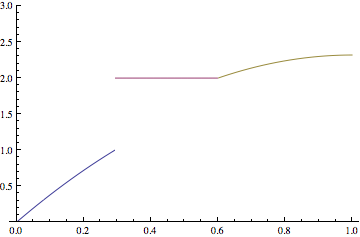
Figure 1: The function ${u}(x)$ for $\gamma=4$

In the specific case, we have (see Figure 1)

$$u(x)=\left\{\begin{aligned} &\frac{1}{2}\left(2\gamma x-\gamma x^{2}\right)\quad&0<x<\xi\\ &2\quad&\xi<x<\eta\\ &\frac{\gamma\eta^{2}}{2}-\gamma\eta-\frac{\gamma x^{2}}{2}+\gamma x+2\quad&\eta<x<1.\end{aligned}\right.$$

We now show that this is not possible because the functional takes a lower value on the solution with only a jump at $x=\xi$. In fact, if we consider the function $\tilde{u}(x)$ defined as follows

$$\tilde{u}(x)=\left\{\begin{aligned} &\frac{1}{2}\left(2\gamma x-\gamma x^{2}\right)\quad&0<x<\xi\\ &\frac{1}{2}\left(-\gamma x^{2}+2\gamma x+2\right)\quad&\xi<x<1\end{aligned}\right.$$

we observe that $u=\tilde{u}$ in $[0,\xi]$, while $u^{\prime}=\tilde{u}^{\prime}=\gamma(1-x)$ for all $x\notin[\xi,\eta]$ and, by explicit computations, we have

$$J(\tilde{u})-J(u)=\gamma^{2}\left[-\frac{\eta}{2}+\frac{\eta^{2}}{2}-\frac{\eta^{3}}{6}+\frac{\xi}{2}-\frac{\xi^{2}}{2}+\frac{\xi^{3}}{6}\right]=\gamma^{2}(\Phi(\eta)-\Phi(\xi))<0,\quad\xi<\eta$$

where $\Phi(s)=-\frac{s}{2}+\frac{s^{2}}{2}-\frac{s^{3}}{6}$ is strictly decreasing, since $\Phi^{\prime}(s)=-\frac{1}{2}(s-1)^{2}\leq 0$.

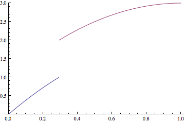
Figure 2: The function $\tilde{u}(x)$ for $\gamma=4$

Actually, the solution is the one shown in Figure 2. Next we show that there exists a unique point $\xi$ such that the minimum is attained. We write the functional $J(u)$, on a generic solution with a single jump from the value $u=1$ to the value $u=2$ at the point $0<\xi<1$ and such that the Euler equation is satisfied before and after $\xi$. We obtain the following value for the functional (in terms of the point $\xi$)

$$J(u)=F(\xi)=\frac{\gamma^{2}\xi^{3}}{8}-\frac{\gamma^{2}\xi^{2}}{2}+\frac{\gamma^{2}\xi}{2}-\frac{\gamma^{2}}{6}+\frac{3\gamma\xi}{2}-2\gamma+\frac{1}{2\xi}.$$

We observe that, $\forall\,\gamma>2$

$$F(0^{+})=+\infty\qquad\text{and}\qquad F(1)=-\frac{\gamma^{2}}{24}-\frac{\gamma}{2}+\frac{1}{2}<0.$$

To study the behavior of $F(\xi)$ one has to solve some fourth order equations (this could be possible in an explicit but cumbersome way), so we prefer to make a qualitative study. We evaluate

$$F^{\prime}(\xi) =\frac{3\gamma^{2}\xi^{2}}{8}-\gamma^{2}\xi+\frac{\gamma^{2}}{2}+\frac{3\gamma}{2}-\frac{1}{2\xi^{2}},$$

$$F^{\prime\prime}(\xi) =\frac{3\gamma^{2}\xi}{4}-\gamma^{2}+\frac{1}{\xi^{3}},$$

$$F^{\prime\prime\prime}(\xi) =\frac{3\gamma^{2}}{4}-\frac{3}{\xi^{4}},$$

hence we have that

$$F^{\prime\prime\prime}(\xi)<0\quad\text{ if and only if }\quad 0<\xi<\sqrt{\frac{2}{\gamma}}<1.$$

Consequently the function $F^{\prime\prime}(\xi)$, which nevertheless satisfies $\forall\,\gamma>2$

$$F^{\prime\prime}(0^{+})=+\infty,\qquad F^{\prime\prime}(1)=1-\frac{\gamma^{2}}{4}<0,$$

has a unique negative minimum at the point $\sqrt{\frac{2}{\gamma}}$.

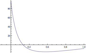
Figure 3: $F^{\prime\prime}(\xi)$ for $\gamma=4$

From this, we deduce that there exists one and only one point $0<\xi_{0}<\sqrt{\frac{2}{\gamma}}$ such that

$$F^{\prime\prime}(\xi)>0 \qquad 0<\xi<\xi_{0}$$

$$F^{\prime\prime}(\xi)<0 \qquad\xi_{0}<\xi\leq 1.$$

From the sign of $F^{\prime\prime}$ we get that $F^{\prime}$ is strictly increasing in $(0,\xi_{0})$ and decreasing in $(\xi_{0},1)$. Next $\forall\,\gamma>2$

$$F^{\prime}(0^{+})=-\infty,\qquad F^{\prime}(1)=-\frac{\gamma^{2}}{8}+\frac{3\gamma}{2}-\frac{1}{2}\qquad$$

hence, in the case that

$$-\frac{\gamma^{2}}{8}+\frac{3\gamma}{2}-\frac{1}{2}>0\quad\text{ that is }\gamma<2\left(3+2\sqrt{2}\right)\sim 11.656...,$$

then $F^{\prime}$ has a single zero $\xi_{1}\in(0,\xi_{0})$ and, being a change of sign, $\xi_{1}$ is a point of absolute minimum for $F(\xi)$.

If $\gamma\geq 2\left(3+2\sqrt{2}\right)$ the above argument fails.

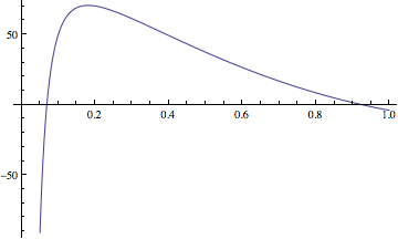
Figure 4: $F^{\prime}(\xi)$ for $\gamma=14$

In this case we can observe that

$$F^{\prime}(1/\gamma)=\frac{\gamma}{2}+\frac{3}{8}>0,$$

hence $F^{\prime}(1)$, which is negative at $\xi=1$ and near $\xi=0$ vanishes exactly two times, at the point $\xi_{1}$, which is a point of local minimum and at another point $\xi_{2}>\xi_{1}$, which is a point of local maximum. Hence, to find the absolute minimum, we have to compare the value of $F(\xi_{1})$ with that of $F(1)$.

In particular, we have that $\xi_{1}<\sqrt{2/\gamma}$ hence, we can show that the minimum is not at $\xi=1$ simply by observing that we can find at least a point where $F(\xi)<F(1)$ and this point is $\sqrt{2/\gamma}$. In fact

$$M(\gamma):=F(\sqrt{2/\gamma})-F(1)=\frac{\gamma^{3/2}}{\sqrt{2}}-\frac{\gamma^{2}}{8}-\frac{5\gamma}{2}+2\sqrt{2}\sqrt{\gamma}-\frac{1}{2}\leq 0.$$

In particular $M(2)=0$ and

$$M^{\prime}(\gamma)=\frac{1}{4}\left(-\gamma+3\sqrt{2}\sqrt{\gamma}+\frac{4\sqrt{2}}{\sqrt{\gamma}}-10\right)<0.$$

This follows since by the substituting $\sqrt{\gamma}\to\chi$, we have to control the sign of the cubic

$$\tilde{M}(\chi)=-\chi^{3}+3\sqrt{2}\chi^{2}-10\chi+4\sqrt{2}$$

which is negative for all $\chi\geq 1$, since $\tilde{M}(1)=-11+7\sqrt{2}$, while

$$\tilde{M}^{\prime}(\chi)=-3\chi^{2}+6\sqrt{2}\chi-10,$$

is a parabola with negative minimum. ∎

Remark 69.

It could be interesting to study this problem in dimension bigger that one, namely, to minimize

$$J\text{\textdegree}(u)=\sqint_{\Omega}\left(\frac{1}{2}a(u)|Du(x)|^{2}-\gamma u(x)\right)\,dx$$ (55)

in the set

$$\left\{v\in V_{\Lambda}(\Omega)\,|\,\forall x\in\Xi^{*},\,u(x)=0\,\right\}$$

and in particular to investigate the structure of the singular set of $u$, both in the general case and in some particular situations in which it is possible to find explicit solutions (e.g. $\Omega=B_{R}(0)$).

References

- [1] Benci V., An algebraic approach to nonstandard analysis, in: Calculus of Variations and Partial differential equations, (G.Buttazzo, et al., eds.), Springer, Berlin (1999), 285-326.
- [2] Benci V., Ultrafunctions and generalized solutions, Adv. Nonlinear Stud. 13, (2013), 461–486, arXiv:1206.2257.
- [3] V. Benci, S. Galatolo, M. Ghimenti, An elementary approach to Stochastic Differential Equations using the infinitesimals, in Contemporary Mathematics 530, Ultrafilters across Mathematics, American Mathematical Society, (2010), p. 1-22.
- [4] Benci V., Di Nasso M., Alpha-theory: an elementary axiomatic for nonstandard analysis, Expo. Math. 21, (2003), 355-386.
- [5] Benci V., Luperi Baglini L., A model problem for ultrafunctions, in: Variational and Topological Methods: Theory, Applications, Numerical Simulations, and Open Problems. Electron. J. Diff. Eqns., Conference 21 (2014), 11-21.
- [6] Benci V., Luperi Baglini L., Basic Properties of ultrafunctions, in: Analysis and Topology in Nonlinear Dierential Equations (D. G. Figuereido, J. M. do O, C. Tomei eds.), Progress in Nonlinear Dierential Equations and their Applications, 85 (2014), 61-86.
- [7] Benci V., Luperi Baglini L., Ultrafunctions and applications, DCDS-S, Vol. 7, No. 4, (2014), 593-616. arXiv:1405.4152.
- [8] Benci V., Luperi Baglini L., A non archimedean algebra and the Schwartz impossibility theorem,, Monatsh. Math. (2014), 503-520.
- [9] Benci V., Luperi Baglini L., Generalized functions beyond distributions, AJOM 4, (2014), arXiv:1401.5270.
- [10] Benci V., Luperi Baglini L., A generalization of Gauss’ divergence theorem, in: Recent Advances in Partial Dierential Equations and Applications, Proceedings of the International Conference on Recent Advances in PDEs and Applications (V. D. Radulescu, A. Sequeira, V. A. Solonnikov eds.), Contemporary Mathematics (2016), 69-84.
- [11] V. Benci, L. Horsten, S. Wenmackers - Non-Archimedean probability, Milan J. Math. 81 (2013), 121-151. arXiv:1106.1524.
- [12] Boccardo L., Croce, G. - Elliptic partial differential equations, De Gruyter, (2013)
- [13] Colombeau, J.-F. Elementary introduction to new generalized functions. North-Holland Mathematics Studies, 113. Notes on Pure Mathematics, 103. North-Holland Publishing Co., Amsterdam, 1985
- [14] Evans L.C., Gariepy R.F. - Measure theory and fine properties of functions - Studies in Advanced Mathematics. CRC Press, Boca Raton, FL, 1992.
- [15] Keisler H. J., Foundations of Infinitesimal Calculus, Prindle, Weber & Schmidt, Boston, (1976).
- [16] Nelson, E. - Internal Set Theory: A new approach to nonstandard analysis, Bull. Amer. Math. Soc., 83 (1977), 1165–1198.
- [17] Robinson A., Non-standard Analysis,Proceedings of the Royal Academy of Sciences, Amsterdam (Series A) 64, (1961), 432-440.
- [18] Sato, M. , Theory of hyperfunctions. II. J. Fac. Sci. Univ. Tokyo Sect. I 8 (1959) 139-193.
- [19] Sato, M., Theory of hyperfunctions. II. J. Fac. Sci. Univ. Tokyo Sect. I 8 (1960) 387–437.
- [20] Squassina M., Exstence, multiplicity, perturbation and concentration results for a class of quasi linear elliptic problems, Electronic Journal of Differential Equations, Monograph 07, 2006, (213 pages). ISSN: 1072-6691. URL: http://ejde.math.txstate.edu or http://ejde.math.unt.edu ftp ejde.math.txstate.edu