Field Theory of Disordered Elastic Interfaces at 3-Loop Order: Critical Exponents and Scaling Functions

Abstract

For disordered elastic manifolds in the ground state (equilibrium) we obtain the critical exponents for the roughness and the correction-to-scaling up to 3-loop order, i.e. third order in $\varepsilon=4-d$, where $d$ is the internal dimension $d$. We also give the full 2-point function up to order $\varepsilon^{2}$, i.e. at 2-loop order.

1 Introduction

For disordered system the application of the functional renormalization group (FRG) is non-trivial because of the cuspy form of the disorder correlator [1, 2, 3, 4, 5, 6, 7, 8, 9]. In [10] we obtained for a 1-component field ($N=1$) the $\beta$-function to 3-loop order, employing the exact renormalization group and several other techniques. Here we analyze the fixed point: We calculate to 3-loop order the roughness exponent $\zeta$ for random-bond disorder, the universal amplitude for periodic disorder, as well as the RG fixed-point functions and universal correction-to-scaling exponents. We also give the complete functional form of the universal 2-point function up to 2-loop order.

Our results are relevant for a remarkably broad set of problems, from subsequences of random permutations in mathematics [11], random matrices [12, 13] to growth models [14, 15, 16, 17, 18, 19, 20, 21, 22] and Burgers turbulence in physics [23, 24], as well as directed polymers [14, 25] and optimization problems such as sequence alignment in biology [26, 27, 28]. Furthermore, they are very useful for numerous experimental systems, each with its specific features in a variety of situations. Interfaces in magnets [29, 30] experience either short-range disorder (random bond RB), or long range (random field RF). Charge density waves (CDW) [31] or the Bragg glass in superconductors [32, 33, 34, 35, 36] are periodic objects pinned by disorder. The contact line of a meniscus on a rough substrate is governed by long-range elasticity [37, 38, 39, 40, 41]. All these systems can be parameterized by a $N$-component height or displacement field $u(x)$, where $x$ denotes the $d$-dimensional internal coordinate of the elastic object. An interface in the 3D random-field Ising model has $d=2$, $N=1$, a vortex lattice $d=3$, $N=2$, a contact-line $d=1$ and $N=1$. The so-called directed polymer ($d=1$) subject to a short-range correlated disorder potential has been much studied [42] as it maps onto the Kardar-Parisi-Zhang growth model [14, 22, 19] for any $N$, and yields an important check for the roughness exponent, defined below, $\zeta_{\mathrm{eq,RB}}(d=1,N=1)=2/3$. Another important field of applications are avalanches, in magnetic systems known as Barkhausen noise. For applications and the necessary theory see e.g. [43, 44, 45, 46, 47, 48, 49, 50, 51, 52, 53].

Finally, let us note that the fixed points analyzed here are for equilibrium, a.k.a. “statics”. At depinning, both the effective disorder, and the critical exponents change. A notable exception is periodic disorder and its mapping to loop-erased random walks [54], where the disorder force-force correlator $\Delta(u)$ changes by a constant, while all other terms are unchanged, and can be gotten from a simpler scalar field theory, allowing to extend the analysis done here to higher-loop order [54].

2 Model and basic definitions

The equilibrium problem is defined by the partition function ${\cal Z}:=\int{\cal D}[u]\,\exp(-{\cal H}[u]/T)$ associated to the Hamiltonian (energy)

$${\cal H}[u]=\int{\mathrm{d}}^{d}x\,\frac{1}{2}\left[\nabla u(x)\right]^{2}+\frac{m^{2}}{2}\left[u(x)-w\right]^{2}+V\big{(}u(x),x\big{)}\ .$$ (1)

In order to simplify notations, we will often note

$$\int_{x}f(x):=\int{\mathrm{d}}^{d}x\,f(x)\ ,$$ (2)

and in momentum space

$$\int_{q}\tilde{f}(q):=\int\frac{{\mathrm{d}}^{d}q}{(2\pi)^{d}}\tilde{f}(q)\ .$$ (3)

The Hamiltonian (1) is the sum of the elastic energy $\int_{x}\frac{1}{2}\left[\nabla u(x)\right]^{2}$ plus the confining potential $\frac{m^{2}}{2}\int_{x}\left[u(x)-w\right]^{2}$ which tends to suppress fluctuations away from the ordered state $u(x)={w}$, and a random potential $V(u,x)$ which enhances them. $w$ is, up to a factor of $m^{2}$, an applied external force, which is useful to measure the renormalized disorder [55, 9, 56, 57, 37, 52, 58], or properly define avalanches [56, 57, 41, 59, 60, 61, 62]. The resulting roughness exponent $\zeta$

$$\overline{\left<[u(x)-u(x^{\prime})]^{2}\right>}\sim|x-x^{\prime}|^{2\zeta}$$ (4)

is measured in experiments for systems at equilibrium ($\zeta_{\rm eq}$) or driven by a force $f$ at zero temperature (depinning, $\zeta_{\rm dep}$). Here and below $\left<\dots\right>$ denote thermal averages and $\overline{(\dots)}$ disorder ones. In the zero-temperature limit, the partition function is dominated by the ground state, and we may drop the explicit thermal averages. In some cases, long-range elasticity appears, e.g. for a contact line by integrating out the bulk-degrees of freedom [40], corresponding to $q^{2}\to|q|$ in the elastic energy. The random potential can without loss of generality [8, 6] be chosen Gaussian with second cumulant

$$\overline{V(u,x)V(u^{\prime},x^{\prime})}=:R_{0}(u-u^{\prime})\delta^{d}(x-x^{\prime})\ .$$ (5)

$R_{0}(u)$ takes various forms: Periodic systems are described by a periodic function $R_{0}(u)$, random-bond disorder by a short-ranged function, and random-field disorder of variance $\sigma$ by $R(u)\simeq-\sigma|u|$ at large $u$. Although this paper is devoted to equilibrium statics, some comparison with dynamics will be made and it is thus useful to indicate the corresponding equation of motion. Adding a time index to the field, $u(x)\to u(x,t)$, the latter reads

$$\eta\partial_{t}u(x,t)=-\frac{\delta{\cal H}[u]}{\delta u(x,t)}=\nabla_{x}^{2}u(x,t)+m^{2}[w-u(x,t)]+F\left(u(x,t),x\right)\ ,$$ (6)

with friction $\eta$. The (bare) pinning force is $F(u,x)=-\partial_{u}V(u,x)$, with correlator

$$\Delta_{0}(u)=-R_{0}^{\prime\prime}(u)\ .$$ (7)

To average over disorder, we replicate the partition function $n$ times, $\overline{{\cal Z}^{n}}=:{\mathrm{e}}^{-\cal S}$, which defines the effective action $\cal S$,

$${\cal S}[u]=\sum_{a=1}^{n}\frac{1}{2T}\int_{x}\left[\nabla u_{a}(x)\right]^{2}+\frac{m^{2}}{2T}u_{a}(x)^{2}-\frac{1}{2T^{2}}\int_{x}\sum_{a,b=1}^{n}R_{0}\big{(}u_{a}(x)-u_{b}(x)\big{)}\ .$$ (8)

We used the notations introduced in Eqs. (2) and (3). In presence of external sources $j_{a}$, the $n$-times replicated action becomes

$${\cal Z}[j]:=\int\prod_{a=1}^{n}{\cal D}[u_{a}]\,\exp\left(-{\cal S}[u]+\int_{x}\sum_{a}j_{a}(x)u_{a}(x)\right)\ ,$$ (9)

from which all static observables can be obtained. $a$ runs from 1 to $n$, and the limit of zero replicas $n\to 0$ is implicit everywhere.

3 3-loop $\beta$-function

In [10] we derived the functional renormalization group equation for the renormalized, dimensionless disorder correlator $\tilde{R}(u)$. For convenience we restate the $\beta$-function here

$$-m\partial_{m}\tilde{R}(u) = (\varepsilon-4\zeta)\tilde{R}(u)+\zeta u\tilde{R}^{\prime}(u)+\textstyle\frac{1}{2}{\tilde{R}^{\prime\prime}(u)}^{2}-\tilde{R}^{\prime\prime}(u)\tilde{R}^{\prime\prime}(0)$$ (10)

$$+\left({\textstyle\frac{1}{2}}+\varepsilon\,{\cal C}_{1}\right)\Big{[}\tilde{R}^{\prime\prime}(u){\tilde{R}^{\prime\prime\prime}(u)}^{2}-\tilde{R}^{\prime\prime}(0){\tilde{R}^{\prime\prime\prime}({u})}^{2}-\tilde{R}^{\prime\prime}(u){\tilde{R}^{\prime\prime\prime}({0^{+}})}^{2}\Big{]}$$

$$+{\cal C}_{2}\Big{[}{\tilde{R}^{\prime\prime\prime}(u)}^{4}-2{\tilde{R}^{\prime\prime\prime}(u)}^{2}{\tilde{R}^{\prime\prime\prime}(0^{+})}^{2}\Big{]}+{\cal C}_{3}\,\big{[}\tilde{R}^{\prime\prime}(u)-\tilde{R}^{\prime\prime}(0)\big{]}^{2}{\tilde{R}^{\prime\prime\prime\prime}(u)}^{2}\rule{0.0pt}{12.91663pt}$$

$$+{\cal C}_{4}\,\Big{[}\tilde{R}^{\prime\prime}(u){\tilde{R}^{\prime\prime\prime}(u)}^{2}{\tilde{R}^{\prime\prime\prime\prime}(u)}-\tilde{R}^{\prime\prime}(0){\tilde{R}^{\prime\prime\prime}(u)}^{2}{\tilde{R}^{\prime\prime\prime\prime}(u)}-\tilde{R}^{\prime\prime}(u){\tilde{R}^{\prime\prime\prime}(0^{+})}^{2}{\tilde{R}^{\prime\prime\prime\prime}(0)}\Big{]}\ .\qquad\ \ \$$

The coefficients are

$${\cal C}_{1} = \frac{1}{4}+\frac{\pi^{2}}{9}-\frac{\psi^{\prime}(\frac{1}{3})}{6}=-0.3359768096723647...$$ (11)

$${\cal C}_{2} = \frac{3}{4}\zeta(3)+\frac{\pi^{2}}{18}-\frac{\psi^{\prime}(\frac{1}{3})}{12}=0.6085542725335131...$$ (12)

$${\cal C}_{3} = \frac{\psi^{\prime}(\frac{1}{3})}{6}-\frac{\pi^{2}}{9}=0.5859768096723648...$$ (13)

$${\cal C}_{4} = 2+\frac{\pi^{2}}{9}-\frac{\psi^{\prime}(\frac{1}{3})}{6}=1.4140231903276352...\ .$$ (14)

The first line contains the rescaling and 1-loop terms, the second line the 2-loop terms, and the last two lines the three 3-loop terms. Note that $\mathcal{C}_{1}=\frac{1}{4}-\mathcal{C}_{3}$, and ${\cal C}_{4}=2-{\cal C}_{3}=\sqrt{2}-0.000190372...$

4 Summary of main results

Here we summarize the main results. Their derivation is given in the following sections.

4.1 Fixed points and critical exponents

There are four generic distinct disorder classes, corresponding to random-bond, random-field, random-periodic, and generic long-ranged disorder. While we will discuss the details in section 5, we give a summary here.

4.1.1 Random-bond disorder

If the microscopic disorder potential is short-ranged, which corresponds to random-bond disorder in magnetic systems, then the roughness exponent can be calculated in an $\varepsilon=4-d$ expansion:

$$\zeta =\varepsilon\zeta_{1}+\varepsilon^{2}\zeta_{2}+\varepsilon^{3}\zeta_{3}+{\cal O}(\varepsilon^{4})$$ (15)

$$\zeta_{1} =0.2082980628(7)$$ (16)

$$\zeta_{2} =0.006857(8)$$ (17)

$$\zeta_{3} =-0.01075(2)\,.$$ (18)

This series expansion has a rather large third-order coefficient. As we will discuss in the conclusions, this is a little surprising, since one might expect the expansion to converge, contrary to $\varphi^{4}$-theory which has a divergent, but Borel-summable series expansion.

One can use a Padé resummation to improve the expansion. Asking that all Padé coefficients are positive singles out the (2,1)-approximant. It is given by

$$\zeta_{(2,1)}\approx\frac{0.208298\varepsilon+0.333429\varepsilon^{2}}{1+1.56781\varepsilon}+{\cal O}(\varepsilon^{4})\ .$$ (19)

Adding a 4-loop term, and asking that in dimension one the exact result is reproduced, i.e. $\zeta(\varepsilon=3)=2/3$, and choosing the Padé with positive coefficients only, leads to

$$\zeta\approx\frac{0.0021794\varepsilon^{4}+0.333429\varepsilon^{2}+0.208298\varepsilon}{1.56781\varepsilon+1}+{\cal O}(\varepsilon^{4})\ .$$ (20)

Details can be found in section 5.1.

4.1.2 Random-field disorder

The roughness exponent is given

$$\zeta_{\rm RF}=\frac{\varepsilon}{3}\ ,$$ (21)

a result exact to all orders in $\varepsilon$. The amplitude of the 2-point function can be calculated analytically. It is given by

$$\overline{\left<\tilde{u}(q)\tilde{u}(q^{\prime})\right>}=\tilde{c}(d)m^{-d-2\zeta_{\rm RF}}F_{d}(q/m)$$ (22)

$$F_{d}(0)=0\ ,\quad F_{d}(z)\simeq B(d)z^{-d-2\zeta_{\rm RF}}\mbox{~{}~{}for~{}~{}}z\to\infty$$ (23)

$$\tilde{c}(d)\approx\frac{\varepsilon^{\frac{1}{3}}\sigma^{\frac{2}{3}}}{0.283721+0.058367\varepsilon+0.064888\varepsilon^{2}}+{\cal O}(\varepsilon^{\frac{10}{3}})$$ (24)

$$B(d)\approx\frac{1+0.226789\varepsilon}{1+0.560122\varepsilon}+{\cal O}(\varepsilon^{3})\ .$$ (25)

An analytical result is given in Eq. (146) ff. We have again given the Padé approximants with only positive coefficients. Translating to position space yields

$$\frac{1}{2}\overline{\left<[u(x)-u(0)]^{2}\right>}=\frac{-\Gamma(-\tfrac{\varepsilon}{3})\tilde{c}(d)B(d)}{(4\pi)^{\frac{d}{2}}\Gamma\left(\frac{d+8}{6}\right)}\left(\frac{x}{2}\right)^{\!\!\tfrac{2\varepsilon}{3}}\ .$$ (26)

The renormalization-group fixed point function $R(u)$ for the disorder can in this case be calculated analytically to third order in $\varepsilon$. The result, together with details on the calculations is given in section 5.2.

4.1.3 Periodic disorder

For periodic disorder, the 2-point function is always a logarithm in position space, with universal amplitude, corresponding to

$$\zeta_{\mathrm{RP}}=0\ .$$ (27)

The scaling functions are defined as for RF disorder, and read

$$\overline{\left<\tilde{u}(q)\tilde{u}(q^{\prime})\right>}=\tilde{c}(d)m^{-d}F_{d}(q/m)$$ (28)

$$F_{d}(0)=0\ ,\quad F_{d}(z)\simeq B(d)z^{-d}\mbox{~{}for~{}}z\to\infty$$ (29)

$$\tilde{c}(d)\approx\frac{2.19325\varepsilon}{1+0.310238\varepsilon+1.33465\varepsilon^{2}}+{\cal O}(\varepsilon^{4})$$ (30)

$$B(d)\approx\frac{1+0.134567\varepsilon}{1+1.13457\varepsilon}+{\cal O}(\varepsilon^{3})\ .$$ (31)

An analytical result is given in Eq. (147) ff. The Padé approximants are again given with only positive coefficients. Translating to position space yields, with a microscopic cutoff $a$

$$\frac{1}{2}\overline{\left<[u(x)-u(0)]^{2}\right>}=\frac{2\tilde{c}(d)B(d)}{(4\pi)^{\frac{d}{2}}\Gamma(\frac{d}{2})}\ln|x/a|\ .$$ (32)

Details are presented in sections 7.3 and 5.3.

4.2 Correction-to-scaling exponent

The correction-to-scaling exponent $\omega$ quantifies how an observable ${\cal O}$, or a critical exponent, approaches its value at the IR fixed point at length scale $\ell$ or at mass $m$

$${\cal O}-{\cal O}_{\rm fix-point}\sim\ell^{-\omega}\sim m^{\omega}\ .$$ (33)

For the fixed points studied above, the correction-to-scaling exponents are as follows.

Random-Periodic fixed point:

$$\omega_{\rm RP}=-\varepsilon+\frac{2\varepsilon^{2}}{3}-\left(\frac{4\zeta(3)}{3}+\frac{5}{9}\right)\varepsilon^{3}+{\cal O}(\varepsilon^{4})=-\varepsilon\,\frac{1+\left[2\zeta(3)+\frac{1}{6}\right]\varepsilon}{1+\left[2\zeta(3)+\frac{5}{6}\right]\varepsilon}+{\cal O}(\varepsilon^{4})\ .$$ (34)

Random-Bond fixed point:

$$\omega_{\rm RB}\approx-\varepsilon+0.4108\varepsilon^{2}+{\cal O}(\varepsilon^{3})=-\frac{\varepsilon}{1+0.4108\varepsilon}+{\cal O}(\varepsilon^{3})\ .$$ (35)

Random-Field fixed point:

$$\omega_{\rm RF}\approx-\varepsilon+0.1346\varepsilon^{2}+{\cal O}(\varepsilon^{3})=-\frac{\varepsilon}{1+0.1346\varepsilon}+{\cal O}(\varepsilon^{3})\ .$$ (36)

Note that for the RP fixed point, we have given the solution up to 3-loop order. For the other fixed points, we have not attempted to solve the RG equations at this order, as this problem can only be tackled via shooting, which is already difficult at second order. Also, as the 2-loop result seems to be quite reliable, whereas corrections for $\zeta$ are large at 3-loop order, we expect the same to be true for $\omega$, which justifies to stop the expansion at second order.

Finally, we can perform the same analysis at depinning, with results as follows:

Random-Field fixed point at depinning:

$$\omega_{\rm RF}^{\rm depinning}\approx-\varepsilon-0.0186\varepsilon^{2}+{\cal O}(\varepsilon^{3})=-\frac{\varepsilon}{1-0.0186\varepsilon}+{\cal O}(\varepsilon^{3})\ .$$ (37)

Random-Periodic fixed point at depinning:

$$\omega_{\rm RP}^{\rm depinning}=-\varepsilon+\frac{2\varepsilon^{2}}{3}+{\cal O}(\varepsilon^{3})\ .$$ (38)

Strangely, while the RP fixed point at depinning is different, the correction-to-scaling exponent $\omega$ does not change, at least to second order.

4.3 2-point correlation function

The 2-point correlation function can be written as

$${\overline{\langle u(q)u(-q)\rangle}}=m^{-d-2\zeta}\tilde{c}(d)F_{d}({\textstyle\frac{|q|}{m}})\ ,$$ (39)

with a universal amplitude $\tilde{c}(d)$ and a scaling function $F_{d}$ with $F_{d}(0)=1$. We have obtained the scaling function $F_{d}(z)$ in an $\varepsilon$ expansion to second order, see Eqs. (145) and (146).

4.4 Other results

A fixed-point function can also be constructed for generic long-ranged disorder, growing (or decaying) at large distances as $R(u)\simeq u^{\alpha}$, with $\alpha=1$ being random-field disorder discussed above. The idea is the same, in all cases the tail for large $u$ does not get corrected.

5 Fix-point analysis

Irrespective of the precise form of the initial disorder distribution function $R_{0}$ in the bare action, we identify different fix-point classes of the RG equation. Although our description may not be complete, the analysis of fix-point solutions gives insight into possible physical realizations of our simple model [Eq. (1)]. We study a universality class where $R_{0}$ is periodic and in the non-periodic case we distinguish whether $R_{0}$ is short range (random bond disorder) or long range (random field disorder). This chapter follows closely Ref. [6] but generalizes the results to 3-loop order.

In terms of the rescaled disorder distribution function

$$\tilde{R}(u)=(\varepsilon\tilde{I}_{1})m^{-\varepsilon+4\zeta}R(um^{-\zeta})$$ (40)

the $\beta$-function up to 3-loop order was given in Eq. (10).

5.1 Random-bond disorder

In order to describe short-range disorder caused by random bonds we look for a fix-point solution that decays exponentially fast for large fields $u$. To this end we numerically solve the fix-point equation

$$-m\frac{\partial}{\partial m}\tilde{R}(u)=0$$ (41)

order by order in $\varepsilon$. We make the Ansatz

$$\tilde{R}(u) =\varepsilon r_{1}(u)+\varepsilon^{2}r_{2}(u)+\varepsilon^{3}r_{3}(u)+{\cal O}(\varepsilon^{4})$$ (42)

and assume that higher orders in $\varepsilon$ do not contribute to field derivatives of lower orders. Also the roughness exponent is expanded in $\varepsilon$

$$\zeta =\varepsilon\zeta_{1}+\varepsilon^{2}\zeta_{2}+\varepsilon^{3}\zeta_{3}+{\cal O}(\varepsilon^{4})\,.$$ (43)

If $\tilde{R}(u)$ is a fix-point solution of Eq. (10) then $\xi^{4}\tilde{R}(u/\xi)$ is a fix-point solution as well for any $\xi$. Thus, without loss of generality, it is possible to normalize $\tilde{R}(0)=\varepsilon$, that is, we set $r_{1}(0)=1$ and $r_{2}(0)=r_{3}(0)=0$.

Inserting the Ansatz into the fix-point equation we find to lowest, that is, second order in $\varepsilon$

$$0=(1-4\zeta_{1})r_{1}(u)+\zeta_{1}ur_{1}^{\prime}(u)+\frac{1}{2}r_{1}^{\prime\prime}(u)^{2}-r_{1}^{\prime\prime}(u)r_{1}^{\prime\prime}(0)\,.$$ (44)

Together with $r_{1}(0)=1$ this differential equation has a solution for any $\zeta_{1}$. But for only one specific value of $\zeta_{1}$ the solution does not change sign and decays exponentially fast for large $u$. Since $R(u)=R(-u)$ we only consider positive values of $u$.

Numerically, we adopt the following iterative procedure: First, we guess a value for $\zeta_{1}$ and compute the corresponding $r_{1}(u)$. Then we evaluate $r_{1}$ at a large value $u_{\max}$. This is repeated until $r_{1}(u_{\max})=0$. The guessing of $\zeta_{1}$ is improved by calculating $r_{1}(u_{\max})$ for many values of $\zeta_{1}$ and interpolating to zero. In order to circumvent numerical problems at small $u$ we approximate $r_{1}(u)$ by its Taylor expansion up to a finite order for $|u|$ smaller than a gluing point $u_{\mbox{\tiny{glue}}}$. We find

$$\zeta_{1} =0.2082980628(7)$$ (45)

for $u_{\max}=25$. Below $u_{\mbox{\tiny{glue}}}=0.01$ a Taylor expansion of order 30 was used. The result does not depend on the order if high enough, also a reasonable variation of the gluing point $u_{\mbox{\tiny{glue}}}<2$ is within error tolerances (that is, does not change the digits shown here). Of course, the result does depend on $u_{\max}$, but choosing $u_{max}>25$ gives results within error tolerances (checked up to $u_{\max}=50$).

For the higher-loop contributions we also need derivatives of $r_{1}$. Instead of solving the corresponding differential equations we simply take numerical derivatives. This is possible since $r_{1}$ is a smooth function away from zero. Using the obtained $\zeta_{1}$, $r_{1}(u)$, and its derivatives, we can solve for the 2-loop contribution

$$0 =r_{2}(u)-4\zeta_{2}r_{1}(u)-4\zeta_{1}r_{2}(u)+u\zeta_{2}r_{1}^{\prime}(u)+u\zeta_{1}r_{2}^{\prime}(u)+r_{1}^{\prime\prime}(u)r_{2}^{\prime\prime}(u)-r_{1}^{\prime\prime}(0)r_{2}^{\prime\prime}(u)$$ (46)

$$\quad-r_{1}^{\prime\prime}(u)r_{2}^{\prime\prime}(0)+\frac{1}{2}\left(r_{1}^{\prime\prime}(u)-r_{1}^{\prime\prime}(0)\right)r_{1}^{\prime\prime\prime}(u)^{2}-\frac{1}{2}r_{1}^{\prime\prime}(u)r_{1}^{\prime\prime\prime}(0^{+})^{2}$$

with $r_{2}(0)=0$. This equation is solved for $r_{2}(u)$ for different values of $\zeta_{2}$. With an analogous iterative procedure we adjust $\zeta_{2}$ such that $r_{2}(u)$ decays exponentially. The best value is

$$\zeta_{2} =0.006857(8)$$ (47)

as found in [6]. Again, derivatives of $r_{2}(u)$ are computed numerically and put into the 3-loop contribution

$$0 =r_{3}(u)-4\zeta_{3}r_{1}(u)-4\zeta_{2}r_{2}(u)-4\zeta_{1}r_{3}(u)+u\big{[}\zeta_{3}r_{1}^{\prime}(u)+\zeta_{2}r_{2}^{\prime}(u)+\zeta_{1}r_{3}^{\prime}(u)\big{]}$$ (48)

$$\quad-r_{2}^{\prime\prime}(0)r_{2}^{\prime\prime}(u)+{\textstyle\frac{1}{2}}r_{2}^{\prime\prime}(u)^{2}-r_{1}^{\prime\prime}(u)r_{3}^{\prime\prime}(0)-r_{1}^{\prime\prime}(0)r_{3}^{\prime\prime}(u)+r_{1}^{\prime\prime}(u)r_{3}^{\prime\prime}(u)-{\cal C}_{1}r_{1}^{\prime\prime}(u)r_{1}^{\prime\prime\prime}(0)^{2}$$

$$\quad-{\textstyle\frac{1}{2}}r_{2}^{\prime\prime}(u)r_{1}^{\prime\prime\prime}(0)^{2}-{\cal C}_{1}r_{1}^{\prime\prime}(0)r_{1}^{\prime\prime\prime}(u)^{2}+{\cal C}_{1}r_{1}^{\prime\prime}(u)r_{1}^{\prime\prime\prime}(u)^{2}-{\textstyle\frac{1}{2}}r_{2}^{\prime\prime}(0)r_{1}^{\prime\prime\prime}(u)^{2}+{\textstyle\frac{1}{2}}r_{2}^{\prime\prime}(u)r_{1}^{\prime\prime\prime}(u)^{2}$$

$$\quad-2{\cal C}_{2}r_{1}^{\prime\prime\prime}(0)^{2}r_{1}^{\prime\prime\prime}(u)^{2}+{\cal C}_{2}r_{1}^{\prime\prime\prime}(u)^{4}-r_{1}^{\prime\prime}(u)r_{1}^{\prime\prime\prime}(0)r_{2}^{\prime\prime\prime}(0)-r_{1}^{\prime\prime}(0)r_{1}^{\prime\prime\prime}(u)r_{2}^{\prime\prime\prime}(u)+r_{1}^{\prime\prime}(u)r_{1}^{\prime\prime\prime}(u)r_{2}^{\prime\prime\prime}(u)$$

$$\quad-{\cal C}_{4}r_{1}^{\prime\prime}(u)r_{1}^{\prime\prime\prime}(0)^{2}r_{1}^{\prime\prime\prime\prime}(0)-{\cal C}_{4}r_{1}^{\prime\prime}(0)r_{1}^{\prime\prime\prime}(u)^{2}r_{1}^{\prime\prime\prime\prime}(u)+{\cal C}_{4}r_{1}^{\prime\prime}(u)r_{1}^{\prime\prime\prime}(u)^{2}r_{1}^{\prime\prime\prime\prime}(u)+{\cal C}_{3}r_{1}^{\prime\prime}(0)^{2}r_{1}^{\prime\prime\prime\prime}(u)^{2}$$

$$\quad-2{\cal C}_{3}r_{1}^{\prime\prime}(0)r_{1}^{\prime\prime}(u)r_{1}^{\prime\prime\prime\prime}(u)^{2}+{\cal C}_{3}r_{1}^{\prime\prime}(u)^{2}r_{1}^{\prime\prime\prime\prime}(u)^{2}$$

with normalization $r_{3}(0)=0$. With the iterative procedure described above an approximate exponential decay of $r_{3}(u)$ is found for

$$\zeta_{3} =-0.01075(2)\,.$$ (49)

The force correlator $-R^{\prime\prime}(u)$ of the fix-point is plotted on the left side in Fig. 1 for $d=3$, that is, $\varepsilon=1$ in a one-, two-, and 3-loop approximation. There are further renormalizations of the cusp, in particular, the 3-loop contribution seems to counteract the 2-loop contribution such that the 3-loop results is close to the 1-loop result.

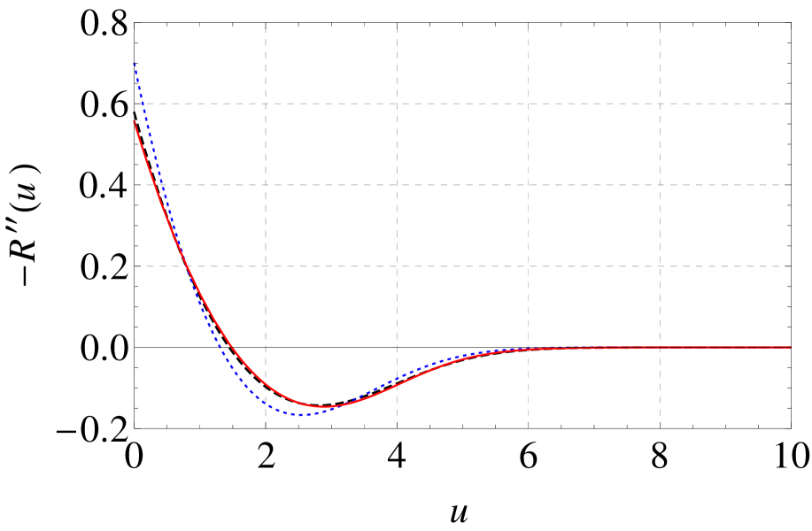
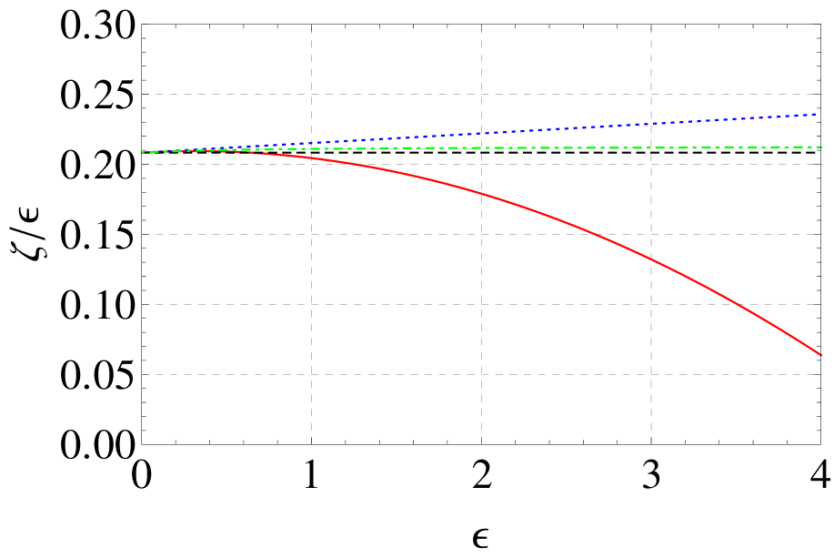
Figure 1: Comparison of results for random bond disorder in 1-loop (black, dashed), 2-loop (blue, dotted), and 3-loop (red, solid) order. Left: Fix point disorder correlator for $d=3$. Right: Dimensional dependence of the roughness exponent normalized with $\varepsilon$. The (2,1)-Padé approximant is plotted in a green dash-dotted line.

The dimensional dependence of the roughness exponent is shown in the right graph of Fig. 1. The corrections in 3-loop order are substantial, for $\varepsilon>1$ they are so large that the $\varepsilon$-expansion is bound to fail. Correspondingly, while the 2-loop results seem to reproduce exact ($d=1$) [63] and simulation results ($d=2,3$) [64], the 3-loop results are worse throughout in this comparison, see Fig. 2. Surprisingly, the (2,1)-Padé-approximant of the 3-loop $\varepsilon$-expansion, which is given by

$$\zeta_{(2,1)}\approx\frac{0.208298\varepsilon+0.333429\varepsilon^{2}}{1+1.56781\varepsilon},$$ (50)

is again very close to the 1-loop result but agrees even better with the reference data. Unfortunately, the third order of a series does not allow to make statements of its asymptotic behavior.

$\zeta_{\rm eq}$	one loop	two loop	three loop	Padé-(2,1)	simulation and exact
$d=3$	0.208	0.215	0.204	0.211	$0.22\pm 0.01$ [64]
$d=2$	0.417	0.444	0.358	0.423	$0.41\pm 0.01$ [64]
$d=1$	0.625	0.687	0.396	0.636	2/3 [63]

Figure 2: Roughness exponent for random bond disorder obtained by an $\varepsilon$-expansion in comparison with exact results and numerical simulations. In the fourth column is an estimate value using a (2,1)-Padé approximant of the 3-loop result.

5.2 Random-field disorder

We consider a class of long-range fix-point solutions with $\tilde{R}(u)\sim-\sigma|u|$ for large $u$. Due to the linear behavior, second and higher derivatives of $\tilde{R}$ do not contribute in the limits $u\to\pm\infty$. Subsequently, all loop corrections to the tail vanish and the reparameterisation terms give $\zeta=\frac{\varepsilon}{3}$ for the roughness exponent to all orders as a prerequisite for the existence of such a fix-point solution.

Following closely the 2-loop calculation [6], we consider $y(u)=-\frac{3}{\varepsilon}\tilde{R}^{\prime\prime}(u)$ and normalize $y(0)=1$. Rewriting the fix-point equation in terms of $y$ and integrating over the interval $[0^{+},u]$ gives (without loss of generality we consider $u>0$)

$$0 =B_{1}+B_{2}\varepsilon+B_{3}\varepsilon^{2}+{\cal O}(\varepsilon^{4})\ .$$ (51)

This is equivalent to taking one derivative of the $\beta$ function (10), and expressing it in terms of $y$. The coefficients $B_{1}$, $B_{2}$ and $B_{3}$ are the 1-, 2-, and 3-loop contributions, given by

$$B_{1}= uy+(1-y)y^{\prime},$$ (52)

$$B_{2}= \frac{1}{6}\Big{[}y^{\prime 2}(y-1)\Big{]}^{\prime}-\frac{1}{6}y^{\prime}y^{\prime}(0)^{2}$$ (53)

and

$$B_{3}= \frac{1}{9}y^{\prime}(0)^{2}\Big{[}(C_{4}y^{\prime\prime}(0)-3C_{1})y+2C_{2}y^{\prime 2}\Big{]}^{\prime}$$

$$+\frac{1}{9}\Big{[}-C_{2}y^{\prime 4}{-}C_{3}(1-y)^{2}y^{\prime\prime 2}+(1-y)y^{\prime 2}(C_{4}{y^{\prime\prime}}-3C_{1})\Big{]}^{\prime}\ .$$ (54)

These equations can be solved analytically, expressing $u$ as a function of $y$. For the 1-loop equation, the solution reads

$$\frac{u^{2}}{2}=y-1-\ln y,$$ (55)

which features the cusp. Higher-loop contributions are obtained by making an ansatz; to 3-loop order we need

$$\frac{u^{2}}{2}=y-1-\ln y-\frac{\varepsilon}{3}F_{2}(y)-\frac{\varepsilon^{2}}{6}F_{3}(y)+{\cal O}(\varepsilon^{3})\ ,\qquad u>0\ .$$ (56)

The inverse function of $u(y)$, $u>0$, is $y(u)$. We make use of the known 2-loop solution [6]

$$F_{2}(y)=2y-1-\frac{1}{2}\ln y+\frac{y}{1-y}\ln y+\mbox{Li}_{2}(1-y)$$ (57)

with boundary conditions up to 2-loop order

$$y^{\prime}(0) =-1-\frac{2}{9}\varepsilon+{\cal O}(\varepsilon^{2})$$ (58)

$$y^{\prime\prime}(0) =\frac{2}{3}+\frac{19}{54}\varepsilon+{\cal O}(\varepsilon^{2})$$

$$y^{\prime\prime\prime}(0) =-\frac{1}{6}-\frac{71}{360}\varepsilon+{\cal O}(\varepsilon^{2})\ .$$

Differentiating the ansatz (56), with respect to $u$ gives an $\varepsilon$-expansion for $y^{\prime}(u)$

$$y^{\prime}(u)=-\frac{uy(u)}{1-y(u)}-\frac{1}{3}\frac{y(u)y^{\prime}(u)}{1-y(u)}\left[\varepsilon\frac{\mathrm{d}}{\mathrm{d}y}F_{2}(y)\Big{|}_{y=y(u)}+\frac{1}{2}\varepsilon^{2}\frac{\mathrm{d}}{\mathrm{d}y}F_{3}(y)\Big{|}_{y=y(u)}\right]+{\cal O}(\varepsilon^{3})\ .$$ (59)

We now insert this expression into Eq. (51), replacing for the moment only $B_{1}$ by its explicit form (52). Then the fix-point condition reads

$$0=\varepsilon\left[B_{2}-\frac{1}{3}y(u)y^{\prime}(u)F_{2}^{\prime}(y(u))\right]+\varepsilon^{2}\left[B_{3}-\frac{1}{6}y(u)y^{\prime}(u)F_{3}^{\prime}(y(u))\right]+{\cal O}(\varepsilon^{3})\ .$$ (60)

The two terms, each enclosed by square brackets, are dealt with separately. We integrate the first term with respect to $u$ and then again insert Eq. (59) to shift the occurrence of $y^{\prime}(u)$ to a higher order in $\varepsilon$. Since $F_{2}$ determines the 2-loop fixed point, the expression is of order $\varepsilon$

$$\int_{0^{+}}^{\overline{u}}\mathrm{d}u\left[B_{2}-\frac{1}{3}y(u)y^{\prime}(u)F_{2}^{\prime}(y(u))\right]=:{u}_{1}(y(\overline{u}),\overline{u})\varepsilon+{\cal O}(\varepsilon^{2}).$$ (61)

The function $F_{3}$ can now be determined by considering the $\varepsilon^{2}$-contribution to Eq. (60),

$$B_{3}-\frac{1}{6}F_{3}^{\prime}(y(u))y^{\prime}(u)y(u)+\frac{\mathrm{d}}{\mathrm{d}u}{u}_{1}(y(u),u)=0$$ (62)

and $F_{3}(1)=0$. Dividing by $y(u)$ and integrating over $u$ we find

$$F_{3}(y(u))=6\int^{u}\mathrm{d}u\frac{1}{y(u)}\left[B_{3}+\frac{\mathrm{d}}{\mathrm{d}u}{u}_{1}(y(u),u)\right]\ .$$ (63)

(The lower bounds from the left and right-hand side cancel.) The integral on the right-hand-side is evaluated by first integrating

$$\Psi(u)=\int^{u}\mathrm{d}u\left[B_{3}+\frac{\mathrm{d}}{\mathrm{d}u}{u}_{1}(y(u),u)\right]$$ (64)

and then replacing $y^{\prime}(u)$ and $y^{\prime\prime}(u)$ by Eq. (59) and $u^{2}$ by Eq. (56) to zeroth order in $\varepsilon$. The remaining integral

$$\int\mathrm{d}u\frac{1}{y(u)}\frac{\mathrm{d}}{\mathrm{d}u}\Psi(u)=\tilde{F}_{3}(y(u))$$ (65)

can be evaluated with the help of Mathematica and is a function of $y(u)$ only. We find

$$F_{3}(y)=\tilde{F}_{3}(y)-\tilde{F}_{3}(1)=f_{0}+f_{1}\ln y+f_{2}(\ln y)^{2}+f_{3}\ln y\ln(1-y),$$ (66)

where

$$f_{0} =\frac{4+\frac{4\pi^{2}}{9}-\frac{2}{3}\gamma_{\frac{1}{3}}-2\zeta(3)}{(1-y)^{2}}-\frac{48-\pi^{2}-30\zeta(3)}{9(1-y)}-\frac{1}{18}\Big{[}6-3\gamma_{\frac{1}{3}}+(57+8\pi^{2})\zeta(3)\Big{]}$$

$$~{}~{}~{}+(1-y)\Big{[}-\frac{4}{9}\pi^{2}+\frac{2}{3}+\frac{2}{3}\gamma_{\frac{1}{3}}+4\zeta(3)\Big{]}+\frac{2}{3}\left(4\zeta(3)-\frac{2-y}{1-y}\right)\mbox{Li}_{2}(y)-\frac{2}{3}\mbox{Li}_{3}(1-y)$$ (67)

with $\gamma_{\frac{1}{3}}=\psi^{\prime}({\textstyle\frac{1}{3}})$. Furthermore,

$$f_{1} =\frac{23}{18}-\frac{38\pi^{2}}{81}+\frac{19}{27}\gamma_{\frac{1}{3}}+\frac{4}{27}\frac{-2\pi^{2}+3(9+\gamma_{\frac{1}{3}}-15\zeta(3))}{1-y}-\frac{2}{27}\frac{180+4\pi^{2}-6\gamma_{\frac{1}{3}}-117\zeta(3)}{(1-y)^{2}}$$ (68)

$$~{}~{}~{}+\frac{8+\frac{8\pi^{2}}{9}-\frac{4}{3}\gamma_{\frac{1}{3}}-4\zeta(3)}{(1-y)^{3}}+2\zeta(3)$$

$$f_{2} =\frac{4+\frac{4\pi^{2}}{9}-\frac{2}{3}\gamma_{\frac{1}{3}}-2\zeta(3)}{(1-y)^{4}}-\frac{8+\frac{8\pi^{2}}{27}-\frac{4}{9}\gamma_{\frac{1}{3}}-\frac{16}{3}\zeta(3)}{(1-y)^{3}}+\frac{4-\frac{4\pi^{2}}{27}+\frac{2}{9}\gamma_{\frac{1}{3}}-4\zeta(3)}{(1-y)^{2}}+\frac{2}{3}\zeta(3)$$ (69)

$$f_{3} =-\frac{2}{3}-\frac{\frac{2}{3}}{1-y}+\frac{8}{3}\zeta(3)\ .$$ (70)

The functions $F_{2}$ and $F_{3}$ correct the cusp without destroying it, since both have a finite Taylor expansion around $y=1$,

$$F_{2}(y)= \,\frac{2}{3}(1-y)^{2}+\frac{13}{36}(1-y)^{3}+\frac{19}{80}(1-y)^{4}+\frac{13}{75}(1-y)^{5}+\frac{17}{126}(1-y)^{6}+\frac{43}{392}(1-y)^{7}$$

$$\,+\frac{53}{576}(1-y)^{8}+\frac{32}{405}(1-y)^{9}+\frac{19}{275}(1-y)^{10}+{\cal O}(1-y)^{11}$$ (71)

$$F_{3}(y)= \,-2.08216(1-y)^{2}-0.949217(1-y)^{3}-0.541283(1-y)^{4}-0.350724(1-y)^{5}$$

$$\,-0.247215(1-y)^{6}-0.185059(1-y)^{7}-0.144938(1-y)^{8}-0.117575(1-y)^{9}$$

$$\,-0.0980832(1-y)^{10}+{\cal O}(1-y)^{11}\ .$$ (72)

Both Taylor-expansions seem to be convergent in the whole range of $y$. The 3-loop contribution has the opposite sign as the 2-loop contribution. For $\varepsilon=1$ the 3-loop result corrects the 1-loop result in a different direction than the 2-loop result, see Fig. 3. The 3-loop contribution is larger than the 2-loop contribution, and the 3-loop result is closer to the 1-loop result.

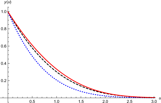
Figure 3: Fix-point solution $y(u)=-\frac{3}{\varepsilon}\tilde{R}^{\prime\prime}(u)$ for $\varepsilon=1$ in the case of random-field disorder. Comparison of 1-loop (dashed black), 2-loop (blue dotted), and 3-loop (red line).

If $\tilde{\Delta}(u):=-\tilde{R}^{\prime\prime}(u)=\frac{\varepsilon}{3}y(u)$ is a fix-point solution, then

$$\tilde{\Delta}(u)=-\tilde{R}^{\prime\prime}(u)=\frac{\varepsilon}{3}\xi^{2}y({\textstyle\frac{u}{\xi}})$$ (73)

is a fix-point solution for any $\xi$ as well. We choose $\xi$ to set the normalization of the fix-point function such that $\tilde{R}(u)\sim-\tilde{\sigma}|u|$ for large $u$, where $\tilde{\sigma}=(\varepsilon\tilde{I}_{1})\sigma$. This ensures $R(u)=\frac{1}{\varepsilon\tilde{I}_{1}}m^{\varepsilon-4\zeta}\tilde{R}(um^{\zeta})\sim-\sigma|u|$, with $\zeta=\frac{\varepsilon}{3}$ . The constant $\xi$ is determined by

$$\tilde{\sigma}\overset{!}{=}-\int_{0}^{\infty}\mathrm{d}u\;\tilde{R}^{\prime\prime}(u)=\frac{\varepsilon}{3}\xi^{3}\int_{0}^{\infty}\mathrm{d}u\;y(u)=\frac{\varepsilon}{3}\xi^{3}\int_{0}^{1}\mathrm{d}y\;u(y)=\frac{\varepsilon}{3}\xi^{3}{{\cal I}_{y}}\ .$$ (74)

The (implicit) solution $u(y)$ is given by the ansatz (56). Numerically, the integral is given by

$${{\cal I}_{y}} =\int_{0}^{1}\mathrm{d}y\;u(y)\approx 0.775304-0.139455\varepsilon+0.17420\varepsilon^{2}+{\cal O}(\varepsilon^{3})\ .$$ (75)

With this fix-point solution, we calculate the universal amplitude as

$$\tilde{c}(d)=m^{d+2\zeta}\langle u(0)u(0)\rangle=-\frac{1}{\varepsilon\tilde{I}_{1}}\tilde{R}^{\prime\prime}(0)=\frac{1}{(\varepsilon\tilde{I}_{1})^{\frac{1}{3}}}\left(\frac{\varepsilon}{3}\right)^{\frac{1}{3}}\sigma^{\frac{2}{3}}{{\cal I}_{y}}^{-\frac{2}{3}}\ .$$ (76)

Using formulas (128)–(130), we obtain

$$\tilde{c}(d)\approx\varepsilon^{\frac{1}{3}}\sigma^{\frac{2}{3}}\Big{[}3.52459-0.72508\varepsilon-0.65692\varepsilon^{2}+{\cal O}(\varepsilon^{3})\Big{]}\ .$$ (77)

For $\varepsilon<0.5$ the 3-loop solution is relatively close to the 2-loop contribution. For larger $\varepsilon$ it deviates substantially and even changes sign for $\varepsilon\approx 1.83$, see Fig.4.

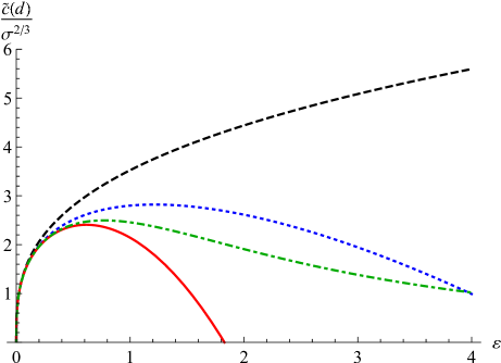
Figure 4: Dimensional dependence of the universal amplitude for random-field disorder. Comparison of 1-loop (dashed black), 2-loop (blue dotted), and 3-loop (red line). The green dot-dashed line is the (0,2)-Padé approximant of the 3-loop solution.

The comparison with the exact result in $d=0$ dimensions [65] may be far fetched in an $\varepsilon=4-d$ expansion. The 1- and 3-loop results are far off from the exact result, but the 2-loop result comes surprisingly close, see Fig. 5. More convincingly and even closer to the exact result is the (0,2)-Padé approximant of the 3-loop result, taking out the prefactor of $\varepsilon^{1/3}$, which is the unique approximant with only positive coefficients,

$$\tilde{c}(d)_{(0,2)}\approx\frac{\varepsilon^{\frac{1}{3}}\sigma^{\frac{2}{3}}}{0.283721+0.058367\varepsilon+0.064888\varepsilon^{2}}\ .$$ (78)

$\tilde{c}(d)\sigma^{-\frac{2}{3}}$	one loop	two loop	three loop	Padé-(0,2)	exact
$d=3$	3.525	2.800	2.143	2.457
$d=2$	4.441	2.614	-0.697	1.909
$d=1$	5.083	1.946	-6.581	1.383
$d=0$	5.595	0.991	-15.694	1.021	$\approx 1.054$ [65]

Figure 5: Universal amplitude for random field disorder obtained by an $\varepsilon$-expansion in comparision with the exact result. In the fourth column is the estimated value using a (0,2)-Padé approximant of the 3-loop result.

5.3 Periodic systems

In order to allow for a periodic solution of the fix-point equation we set $\zeta=0$. Further we assume a period of one; we can use the reparametrization invariance in Eq. (73) to adjust to other periods. The ansatz

$$\tilde{R}(u) =(a_{1}\varepsilon+a_{2}\varepsilon^{2}+a_{3}\varepsilon^{3}+\ldots)+(b_{1}\varepsilon+b_{2}\varepsilon^{2}+b_{3}\varepsilon^{3}+\ldots)u^{2}(1-u)^{2}+{\cal O}(\varepsilon^{4})$$ (79)

works to all orders in $\varepsilon$. This can be seen from the following observations: Each further order in a loop-expansion has one more factor of $R(u)$, and 4 more derivatives. So the RG-equations close for a polynomial up to order $u^{4}$, and no higher-order terms in $u$ are needed. This leaves us with 5 terms, $u^{i}$, with $0\leq i\leq 4$. The function must further be even under the transformation $u\to 1-u$. This leaves space in Eq. (79) for one additional term, $cu(1-u)$, where the constant $c$ may depend on $\varepsilon$. However, each term in the $\beta$-function except the first one $\varepsilon R(u)$ has at least two derivatives, so this term would only appear in $\varepsilon R(u)$, and thus must vanish. (It can appear at depinning for different reasons, see [7].) This leads to the fix-point function

$$\tilde{R}^{*}(u) =\frac{\varepsilon}{2592}+\frac{\varepsilon^{2}}{7776}+\varepsilon^{3}\left(-\frac{1}{46656}+\frac{\pi^{2}}{23328}-\frac{\psi^{\prime}({\textstyle\frac{1}{3}})}{15552}+\frac{\zeta(3)}{15552}\right)$$ (80)

$$\quad-(1-u)^{2}u^{2}\left(\frac{\varepsilon}{72}+\frac{\varepsilon^{2}}{108}+\varepsilon^{3}\frac{9+2\pi^{2}-3\psi^{\prime}({\textstyle\frac{1}{3}})-18\zeta(3)}{1944}\right)+{\cal O}(\varepsilon^{4})\ .$$

With numerical coefficients, the function reads

$$\tilde{R}(u) \approx 0.000385802\varepsilon+0.000128601\varepsilon^{2}-0.000170212\varepsilon^{3}$$

$$\quad-(0.0138889\varepsilon+0.00925926\varepsilon^{2}-0.0119262\varepsilon^{3})(1-u)^{2}u^{2}+{\cal O}(\varepsilon^{4})\ .$$ (81)

Similarly as for random-field disorder we obtain the universal amplitude as

$$\tilde{c}(d)=-\frac{1}{\varepsilon\tilde{I}_{1}}\tilde{R}^{\prime\prime}(0)\approx 2.19325\varepsilon-0.680427\varepsilon^{2}-2.71612\varepsilon^{3}+{\cal O}(\varepsilon^{4})\ .$$ (82)

This is the 2-point correlation function at zero momentum. There is a large contribution in 3-loop order with a larger coefficient than at 2-loop order. For $\varepsilon>0.72$ the 3-loop expansion becomes negative (as does the 2-loop expansion for $\varepsilon>3.22$). This makes the $\varepsilon$-expansion questionable in this case, although the (1,2)-Padé approximant remains positive,

$$\tilde{c}(d)_{(1,2)} \approx\frac{2.19325\varepsilon}{1+0.310238\varepsilon+1.33465\varepsilon^{2}}+{\cal O}(\varepsilon^{4})\ .$$ (83)

The results from different truncations in the loop order and the (1,2)-Padé approximant are plotted in Fig. 6. The amplitude of the propagator in the massless limit is given by

$$c(d)\approx 2.19325\varepsilon-2.87367\varepsilon^{2}+0.45(1)\varepsilon^{3}+{\cal O}(\varepsilon^{4})\ ,$$ (84)

with a 3-loop coefficient not as large as the 2-loop coefficient. Here, however, already the 2-loop solution leads to negative values for $\varepsilon>0.76$. The probably best extrapolations is obtained from the (1,2)-Padé approximant

$$c(d)_{{(1,2)}}\approx\frac{2.19325\varepsilon}{1+1.31024\varepsilon+1.510(6)\varepsilon^{2}}+{\cal O}(\varepsilon^{4})\ .$$ (85)

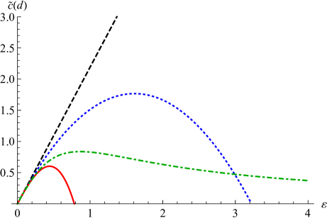
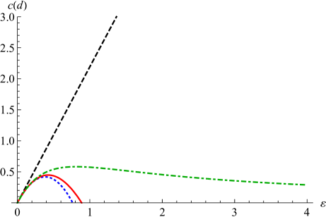
Figure 6: Left: Dimensional dependence of the universal amplitude $\tilde{c}(d)$ in the periodic case. Comparison of 1-loop (dashed black), 2-loop (blue dotted), and 3-loop (red line). The green line corresponds to a (1,2)-Padé approximant of the 3-loop solution. Right: ibid for $c(d)$.

6 The correction-to-scaling exponent $\omega$

The correction-to-scaling exponent $\omega$ controls what happens when a fixed point, here a functional fixed point, is perturbed. In particular, for a fixed point $\Delta^{*}(u)=-\partial_{u}^{2}{{R}^{*}}(u)$ with $\beta[\Delta^{*}]=0$ we consider linear perturbations. Their eigenvalue $\omega$ is determined from the $\cal O(\kappa)$-term in the equation

$$\beta[\Delta^{*}+\kappa z](u)=\omega\kappa\;z(u)+{\cal O}(\kappa^{2})\,.$$ (86)

Since observables, and also scaling functions which determine the critical exponents, in general depend analytically on the coupling constants, a deviation of a critical exponent from the fix-point value scales linearly with the deviation of the coupling constant, or coupling function, from its value at the critical point. In formulas, an observable $\cal O$ or exponent $\alpha$ scales with a length scale $\ell$ as

$${\cal O}-{\cal O}_{\rm fix-point}\sim\alpha-\alpha_{\rm fix-point}\sim R(u)-R_{\rm fix-point}(u)\sim\ell^{-\omega}\ .$$ (87)

This is important for numerical simulations, where $\ell$ is the system size.

For disordered elastic manifolds, this problem has been considered in Ref. [66]. There it was concluded, that two cases have to be distinguished:

• There is the freedom to rescale the field $u$ while at the same time rescaling the disorder correlator. This includes the random-bond and random-field interface models.

• There is no such freedom, since the period is fixed by the microscopic disorder. This is the case for a charge density wave (random periodic problem), but also for the random-field bulk problem, in its treatment via a non-linear sigma model.

In case (a), the two leading eigenvalues and eigenfunctions to linear order in $\varepsilon$ are [66]

$$z_{\rm red}(u) = u\Delta^{\prime}(u)-2\Delta(u)\ ,\qquad~{}~{}~{}~{}~{}~{}~{}~{}~{}~{}~{}~{}~{}\omega_{\rm red}=0\ ,$$ (88)

$$z_{1}(u) = \zeta u\Delta^{\prime}(u)+(\varepsilon-2\zeta)\Delta(u)\ ,\qquad\omega_{1}=-\varepsilon\ .$$ (89)

The first eigenvalue and eigenfunction $z_{\rm red}(u)$ are a consequence of the reparametrization invariance $\Delta(u)\to\kappa^{2}\Delta(u/\kappa)$, and are therefore exact. $z_{\rm red}(u)$ is a redundant operator. $z_{1}(u)$ and $\omega_{1}$ are the dominant eigenfunction and eigenvalue entering into Eq. (87). Both eigenfunctions are given as perturbations of the fixed point $\Delta(u)$ of the force-force correlator. At least for random-field disorder, is was argued [66] that there cannot be any other eigenvalues and eigenfunctions.

In case (b) we can at 1-loop order identify two perturbations, written here as perturbations for the potential-potential correlator $R(u)$:

$$z_{0}(u) = 1\ ,\qquad~{}~{}~{}~{}~{}~{}\omega_{0}=\varepsilon\ ,$$ (90)

$$z_{1}(u) = R(u)\ ,\qquad\omega_{1}=-\varepsilon\ .$$ (91)

6.1 The correction-to-scaling exponent $\omega$ to 2-loop order: General formulas

The 2-loop $\beta$-function is

$$-m\partial_{m}\tilde{\Delta}(u)=(\varepsilon-2\zeta)\Delta(u)+\zeta u\Delta^{\prime}(u)+f_{1}[\Delta,\Delta](u)+f_{2}[\Delta,\Delta,\Delta](u)+...$$ (92)

Both $f_{1}[\Delta]\equiv f_{1}[\Delta,\Delta]$ and $f_{2}[\Delta]\equiv f_{2}[\Delta,\Delta,\Delta]$ are completely symmetric functionals acting locally on the functions $\Delta(u)-\Delta(0)$. More explicitly, we have

$$f_{1}[\Delta]=-\frac{1}{2}\left[(\Delta(u)-\Delta(0))^{2}\right]^{\prime\prime}\ ,$$ (93)

$$f_{2}[\Delta] = \frac{1}{2}\left[(\Delta(u)-\Delta(0))\Delta^{\prime}(u)^{2}\right]^{\prime\prime}-\frac{1}{2}\Delta^{\prime}(0^{+})^{2}\Delta^{\prime\prime}(u)\ .$$ (94)

For different arguments we use the multilinear formulas

$$f(x,y) := \frac{1}{2}\Big{[}f(x+y)-f(x)-f(y)\Big{]}\ ,$$ (95)

$$g(x,y,z) := \frac{1}{6}\Big{[}g(x+y+z)-g(x+y)-g(y+z)-g(x+z)+g(x)+g(y)+g(z)\Big{]}\ ,$$ (96)

$$h(w,x,y,z) := \frac{1}{24}\Big{[}h(w+x+y+z)-h(w+x+y)-h(w+x+z)-h(w+y+z)$$ (97)

$$\qquad-h(x+y+z)+h(w+x)+h(w+y)+h(w+z)+h(x+y)+h(x+z)$$

$$\qquad+h(y+z)-h(w)-h(x)-h(y)-h(z)\Big{]}\ .$$

Consider now $\tilde{\Delta}^{*}(u)$, solution of Eq. (92) with $-m\partial_{m}\tilde{\Delta}^{*}(u)=0$. Setting $\tilde{\Delta}(u)=\tilde{\Delta}^{*}(u)+\kappa z(u)$, we study the flow of the term linear in $\kappa$. Its eigenmodes $z(u)$ with eigenvalues $\omega$ describe the behavior close to the critical point. The eigenvalue-equation to be solved is

$$o(u) := \big{[}\varepsilon-2\zeta-\omega\big{]}z(u)+\zeta uz^{\prime}(u)+2f_{1}[z,\Delta](u)+3f_{2}[z,\Delta,\Delta](u)=0\ .~{}~{}~{}~{}~{}$$ (98)

There are several possible simplifications. First note that if $\Delta(u)$ is a fixed point, also $\kappa^{-2}\Delta(\kappa u)$ is a fixed point. Varying in Eq. (92) the fixed-point condition $-m\partial_{m}\Delta(u)=0$ around $\kappa=1$ yields the redundant or rescaling mode $r(u)$,

$$r(u) = (\varepsilon-2\zeta)\left(u\Delta^{\prime}(u)-2\Delta(u)\right)+\zeta u\left(u\Delta^{\prime}(u)-2\Delta(u)\right)^{\prime}$$ (99)

$$+2f_{1}\left(\Delta(u),u\Delta^{\prime}(u)-2\Delta(u)\right)+3f_{2}\left(\Delta(u),\Delta(u),u\Delta^{\prime}(u)-2\Delta(u)\right)=0\ .\ \ ~{}~{}$$

This equation, as well as a multiple of the vanishing $\beta$-function (92), can be added to Eq. (98). This leaves some freedom to obtain a simpler equation.

We now want to know how the physically relevant correction-to-scaling exponent $\omega=-\varepsilon$ changes to 2-loop order. To this aim we do a loop expansion, starting from what we know,

$$\Delta(u) = \varepsilon\Delta_{1}(u)+\varepsilon^{2}\Delta_{2}(u)+...$$ (100)

$$z(u) = \varepsilon z_{1}(u)+\varepsilon^{2}z_{2}(u)+...$$ (101)

$$z_{1}(u) = \zeta_{1}u\Delta_{1}^{\prime}(u)+(1-2\zeta_{1})\Delta_{1}(u)$$ (102)

$$\zeta = \zeta_{1}\varepsilon+\zeta_{2}\varepsilon^{2}+...$$ (103)

$$\omega = -\varepsilon+\omega_{2}\varepsilon^{2}+...$$ (104)

The 1- and 2-loop orders of the $\beta$-function are given by $\beta=\varepsilon\beta_{1}+\varepsilon^{2}\beta_{2}+{\cal O}(\varepsilon^{3})$ with

$$\beta_{1} = (1-2\zeta_{1})\Delta_{1}(u)+\zeta_{1}u\Delta_{1}^{\prime}(u)+f_{1}\left(\Delta_{1}\right)(u)=0\ ,$$ (105)

$$\beta_{2} = (1-2\zeta_{1})\Delta_{2}(u)+\zeta_{1}u\Delta_{2}^{\prime}(u)-2\zeta_{2}\Delta_{1}(u)+\zeta_{2}u\Delta_{1}^{\prime}(u)+2f_{1}(\Delta_{1},\Delta_{2})+f_{2}(\Delta_{1})(u)\ .~{}~{}~{}~{}~{}~{}~{}~{}~{}~{}~{}$$ (106)

There are many ways a relatively simple differential relation for $\delta z_{2}(u)$ can be written. We start with the ansatz

$$z_{2}(u)=cu\Delta_{1}^{\prime}(u)+d\Delta_{1}(u)+eu\Delta_{2}^{\prime}(u)+f\Delta_{2}(u)+\delta z_{2}(u)\ ,$$ (107)

and consider the following combination

$$o(u)-\beta(u)(2+\varepsilon(4b+2d))-r(u)(\zeta_{1}+b\varepsilon)-g\beta_{2}(u)\varepsilon^{3}=0\ .$$ (108)

For

$$b=c=\frac{2\zeta_{2}}{1-2\zeta_{1}}\ ,\quad d=-\omega_{2}\ ,\quad e=\zeta_{1}\ ,\quad f=2-2\zeta_{1}\ ,\quad g=1\ ,$$ (109)

we get

$$2\left(1-\zeta_{1}\right)\delta z_{2}(u)+\zeta_{1}u\delta z_{2}^{\prime}(u)+2f_{1}\left[\Delta_{1}(u),\delta z_{2}(u)\right]-\omega_{2}\Delta_{1}(u)+\Delta_{2}(u)=0\ .$$ (110)

This is the simplest equation we have been able to find.

At 3-loop order, the problem becomes more complicated. The best equation we found was

$$2f_{1}\Big{(}\Delta_{1}(u),\delta z_{3}(u)\Big{)}+2f_{1}\Big{(}\Delta_{2}(u),\delta z_{2}(u)\Big{)}+3f_{2}\Big{(}\Delta_{1}(u),\Delta_{1}(u),\delta z_{2}(u)\Big{)}$$

$$+\left(\frac{4\zeta_{2}\omega_{2}}{1-2\zeta_{1}}-\omega_{2}^{2}+\omega_{3}\right)f_{1}\Big{(}\Delta_{1}(u),\Delta_{1}(u)\Big{)}+\left(\frac{4\zeta_{2}}{1-2\zeta_{1}}-3\omega_{2}\right)\Delta_{2}(u)+2\Delta_{3}(u)$$

$$-\left(2\zeta_{2}+\omega_{2}\right)\delta z_{2}(u)+\zeta_{2}u\delta z_{2}^{\prime}(u)+\zeta_{1}u\delta z_{3}^{\prime}(u)-2(\zeta_{1}-1)\delta z_{3}(u)=0\ .$$ (111)

For the lack of use in applications (the 3-loop order for the roughness exponent is rather large), we did not try to solve this equation.

We now specify to the main cases of interest.

6.2 Correction-to-scaling exponent at the random-field fixed point

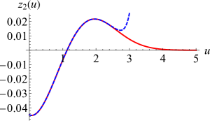
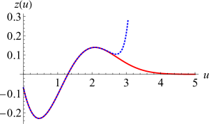
Figure 7: $z_{1}(u)$, $z_{2}(u)$ and $z(u)_{\varepsilon=3}$ for RF, statics. Red (solid) is the numerical solution, blue (dashed) the Taylor expansion around $u=0$.

Using shooting, we find $\omega_{2}=0.1346$, thus

$$\omega\approx-\varepsilon+0.1346\varepsilon^{2}+{\cal O}(\varepsilon^{3})=-\frac{\varepsilon}{1+0.1346\varepsilon}+{\cal O}(\varepsilon^{3})\ .$$ (112)

The corresponding function $\delta z_{2}(u)$ and $z(u)$ at $\varepsilon=3$ are plotted on figure 7. In $d=1$ this gives

$$\omega=-1.97(20)\ ,\qquad d=1\ .$$ (113)

where the error-estimate comes from the deviation of the direct expansion as compared to the Padé approximant.

6.3 Correction-to-scaling exponent at the random-bond fixed point

We find via shooting

$$\omega\approx-\varepsilon+0.4108(1)\varepsilon^{2}+{\cal O}(\varepsilon^{3})=-\frac{\varepsilon}{1+0.4108(1)\varepsilon}+{\cal O}(\varepsilon^{3})\ .$$ (114)

In $d=1$ this gives using the Padé approximant (the direct $\varepsilon$ expansion is not monotonous)

$$\omega\approx-1.344\ ,\qquad d=1\ .$$ (115)

We have checked that the numerical solutions, given on figure 8, integrate to 0 within numerical accuracy, as necessary for a RB fixed point.

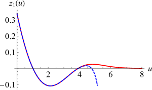
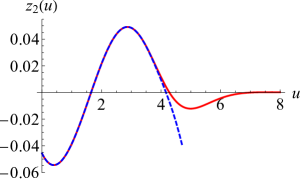
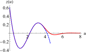
Figure 8: $z_{1}(u)$, $z_{2}(u)$ and $z(u)|_{\varepsilon=3}$ for RB, statics. Red (solid) is the numerical solution, blue (dashed) Taylor expansion.

6.4 Correction-to-scaling exponent for charge-density waves (random-periodic fixed point)

We find that the leading-order perturbation for the random-periodic fix-point (80) closes in the same space spanned by 1 and $[u(1-u)]^{2}$. The correction-to-scaling exponent becomes

$$\omega_{\rm RP}=-\varepsilon+\frac{2\varepsilon^{2}}{3}-\left(\frac{4\zeta(3)}{3}+\frac{5}{9}\right)\varepsilon^{3}+{\cal O}(\varepsilon^{4})=-\varepsilon\,\frac{1+\left[2\zeta(3)+\frac{1}{6}\right]\varepsilon}{1+\left[2\zeta(3)+\frac{5}{6}\right]\varepsilon}+{\cal O}(\varepsilon^{4})\ .$$ (116)

Curiously, all contributions proportional to $\pi^{2}$ and $\psi^{\prime}(1/3)$, present in the coefficients ${\cal C}_{1},...,{\cal C}_{4}$ have canceled. The corresponding eigenfunction, normalized to $\delta R(0)=1$ is

$$\delta R(u)=1-36[u(1-u)]^{2}\left[1+\frac{\varepsilon}{2}+\varepsilon^{2}\frac{8-30\zeta(3)+3\psi^{\prime}(\frac{1}{3})-2\pi^{2}}{18}+{\cal O}(\varepsilon^{3})\right]\ .$$ (117)

Up to 2-loop order, the exponent $\omega$ is the same for depinning.

6.5 Correction-to-scaling exponent for depinning (random-field fixed point)

For completeness and usefulness in applications, we also give the correction-to-scaling exponent at depinning, using the $\beta$-function of [7, 8]. Via shooting, we find $\omega_{2}=-0.0186$, thus

$$\omega\approx-\varepsilon-0.0186\varepsilon^{2}+{\cal O}(\varepsilon^{3})=-\frac{\varepsilon}{1-0.0186\varepsilon}+{\cal O}(\varepsilon^{3})\ .$$ (118)

The corresponding function $\delta z_{2}(u)$ and $z(u)$ at $\varepsilon=3$ are plotted on figure 9. In $d=1$ this gives

$$\omega=-3.17(1)\ ,\qquad d=1\ .$$ (119)

where the error-estimate comes from the difference of the Padé approximant to the direct expansion.

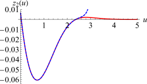
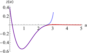
Figure 9: $z_{1}(u)$, $z_{2}(u)$ and $z(u)|_{\varepsilon=3}$ for RF, depinning. Red (solid) is the numerical solution, blue (dashed) the Taylor expansion.

7 2-point correlation function

7.1 2-loop expression

As a prototype physical observable we calculate the 2-point correlation function to 2-loop order in an $\varepsilon$-expansion. This function reads

$$\overline{\langle u(x)u(y)\rangle}_{V}=Tg(x,y)-{\int_{z,z^{\prime}}g(x,z)g(y,z^{\prime})}R^{\prime\prime}[0^{+}](z,z^{\prime})\,.$$ (120)

The expression $R^{\prime\prime}[0^{+}](z,z^{\prime})$ denotes the second functional derivative of $R[u]$ with respect to $u(z)$ and $u(z^{\prime})$ that is evaluated for $u(x)=\mbox{const}\to 0$. Its expansion to 2-loop order has been calculated in [10] and reads

$$R^{\prime\prime}[0^{+}](z,z^{\prime})=R^{\prime\prime}(0^{+})\delta(z-z^{\prime})+\tilde{R}^{\prime\prime}[0^{+}](z,z^{\prime})\,,$$ (121)

where the non-local part is given by

$$\tilde{R}^{\prime\prime}[0^{+}](z_{1},z_{2}) =\delta_{z_{1}z_{2}}\Big{[}-I_{1}R^{\prime\prime\prime}(0^{+})^{2}+(5I_{1}^{2}-4I_{A})R^{\prime\prime\prime}(0^{+})^{2}R^{\prime\prime\prime\prime}(0^{+})\Big{]}$$ (122)

$$+g(z_{1},z_{2})^{2}\Big{[}R^{\prime\prime\prime}(0^{+})^{2}-6I_{1}R^{\prime\prime\prime}(0^{+})^{2}R^{\prime\prime\prime\prime}(0^{+})\Big{]}$$

$$+2g(z_{1},z_{2})R^{\prime\prime\prime}(0^{+})^{2}R^{\prime\prime\prime\prime}(0^{+})\int_{x}\;g(x,z_{1})g(x,z_{2})\big{[}g(x,z_{1})+g(x,z_{2})\big{]}$$

$$+R^{\prime\prime\prime}(0^{+})^{2}R^{\prime\prime\prime\prime}(0^{+})\int_{x}\;g(x,z_{1})^{2}g(x,z_{2})^{2}.$$

Inserting into Eq. (120) and taking the Fourier transform gives at $T=0$

$$g(q)^{-2}\overline{\langle u(q)u(-q)\rangle}_{V} =-R^{\prime\prime}(0^{+})+R^{\prime\prime\prime}(0^{+})^{2}\big{[}I_{1}-I_{1}(q)\big{]}$$ (123)

$$\quad-R^{\prime\prime\prime}(0^{+})^{2}R^{\prime\prime\prime\prime}(0^{+})\big{[}(I_{1}-I_{1}(q))^{2}+4{\Phi_{2,\varepsilon}}(q)\big{]}\ .$$

As before $I_{1}=I_{1}(0)$, $I_{A}=I_{A}(0)$, and $\Phi_{2,\varepsilon}(q)=I_{A}(q)-I_{A}+I_{1}^{2}-I_{1}I_{1}(q)$ with

$$I_{1}(q) =\;\stackrel{{\scriptstyle q}}{{\longrightarrow}}\!\!\!-\!\!\!-\!\!\!\!\parbox{29.29259pt}{\hskip 3.44444pt\includegraphics[scale={0.35}]{1loop}\hskip 3.44444pt}\!\!\!\!\!\!\longrightarrow\!\!\!-\!\!\!-=\int_{p}\;g(p)g(p+q)$$ (124)

$$I_{A}(q) =\;\raisebox{-10.243pt}{$\stackrel{{\scriptstyle q}}{{\longrightarrow}}\!\!\!-\!\!\!-\!\!\!$}\parbox{29.29259pt}{\hskip 3.44444pt\includegraphics[scale={0.35}]{LH}\hskip 3.44444pt}\!\!\!\!\!\!\!\!\!\raisebox{15.07996pt}{${\longrightarrow}\!\!\!-\!\!\!-\!\!\!$}=\int_{p_{1},p_{2}}g(p_{1})g(p_{2})g(p_{1}+p_{2})g(p_{1}+q).$$ (125)

The first line in Eq. (123) is the tree and 1-loop contribution, already calculated in [6]. The second line is the 2-loop contribution, again with a non-vanishing limit $R^{\prime\prime\prime}(0^{+})^{2}$. Note that the momentum could go through the non-trivial 2-loop diagram $I_{A}$ in two different ways, but only the one in Eq. (125) contributes to the 2-point function.

7.2 Integrals

Let us start out with the normalization factors used throughout this work. Consider the 1-loop integral

$$\tilde{I}_{1}=\parbox{29.29259pt}{\hskip 3.44444pt\includegraphics[scale={0.35}]{1loop}\hskip 3.44444pt}\Big{|}_{m=1}=\int_{k}\;{g(k)^{2}}\Big{|}_{m=1}=\int\frac{{\mathrm{d}}^{d}k}{(2\pi)^{d}}\frac{1}{(k^{2}+1)^{2}}\ .$$ (126)

Using a Feynman-representation for the propagator yields

$$\tilde{I}_{1}=\int\frac{{\mathrm{d}}^{d}k}{(2\pi)^{d}}\int_{0}^{\infty}{\mathrm{d}}\alpha\,\alpha\,{\mathrm{e}}^{-\alpha(k^{2}+1)}=\int\frac{{\mathrm{d}}^{d}k}{(2\pi)^{d}}{\mathrm{e}}^{-k^{2}}\times\int_{0}^{\infty}{\mathrm{d}}\alpha\,\alpha^{1-d/2}\,{\mathrm{e}}^{-\alpha}\ .$$ (127)

Let us note, with $d=4-\varepsilon$

$${\cal N}:=\int\frac{{\mathrm{d}}^{d}k}{(2\pi)^{d}}{\mathrm{e}}^{-k^{2}}=\frac{1}{(4\pi)^{\frac{d}{2}}}\ ,$$ (128)

$$\int_{0}^{\infty}{\mathrm{d}}\alpha\,\alpha^{1-d/2}\,{\mathrm{e}}^{-\alpha}=\Gamma(2-\tfrac{d}{2})=\Gamma(\tfrac{\varepsilon}{2})=\frac{2}{\varepsilon}\Gamma(1+\tfrac{\varepsilon}{2})\ .$$ (129)

This yields

$$\varepsilon\tilde{I}_{1}={\cal N}\times 2\Gamma(1+\tfrac{\varepsilon}{2})={{\cal N}}\times\left[2-\gamma_{\rm E}\varepsilon+\frac{1}{24}(6\gamma_{\rm E}^{2}+\pi^{2})\varepsilon^{2}+{\cal O}(\varepsilon^{3})\right]\ .$$ (130)

There are therefore two convenient choices for normalizations: Either we normalize everything by $\varepsilon\tilde{I}_{1}$: then $\tilde{I}_{1}$ will be effectively $1/\varepsilon$, without higher-loop corrections. Or we normalize by ${\cal N}$, which takes out the factor from the Gauss integration. We use whatever is more convenient.

We now turn to the evaluation of $I_{1}(q)$ and $I_{A}(q)$. The 1-loop integral in presence of an external momentum can be parameterized by $I_{1}(q)=\frac{1}{m^{\varepsilon}}\tilde{I}_{1}({\textstyle\frac{q}{m}})$ with

$$\tilde{I}_{1}(z) =\tilde{I}_{1}(0)\;{}_{2}F_{1}(2-d/2,1,3/2,-z^{2}/4)$$ (131)

$$={\tilde{I}_{1}(0)\int\limits_{0}^{1}{\mathrm{d}}y\;\left[1+y(1-y)z^{2}\right]^{-\frac{\varepsilon}{2}}\ .}$$ (132)

Using the series expansion of the hypergeometric function in Eq. (131) or an expansion in $\varepsilon$ of the integrand in Eq. (132), we find

$$\tilde{I}_{1}(z) = \tilde{I}_{1}(0)\Bigg{\{}1+\varepsilon\left(1-\frac{\sqrt{4+z^{2}}}{z}\mbox{asinh}(z/2)\right)$$ (133)

$$+ \varepsilon^{2}\Bigg{[}1+\frac{\sqrt{4+{z^{2}}}}{4z}\Bigg{(}\text{Li}_{2}\!\Big{(}\tfrac{1}{2}-\tfrac{z}{2\sqrt{{z^{2}}+{4}}}\Big{)}-\text{Li}_{2}\!\Big{(}\tfrac{1}{2}+\tfrac{z}{2\sqrt{{z^{2}}{+}{4}}}\Big{)}+\left(\ln(z^{2}{+}4){-}4\right)\mbox{asinh}(z/2)\Bigg{)}\Bigg{]}$$

$$+ {\cal O}(\varepsilon^{3})\Bigg{\}}\ .$$

All singular contributions of $\tilde{I}_{1}(z)$ are present for $z=0$, where $\tilde{I}_{1}(0)={\cal N}[{\textstyle\frac{2}{\varepsilon}}-\gamma_{\mbox{\tiny{E}}}+{\cal O}(\varepsilon)]$. Thus, the difference $I_{1}-I_{1}(q)$ is finite in the limit of $\varepsilon\to 0$. The asymptotics for large $z$ is given by

$$\tilde{I}_{1}(z)\simeq\tilde{I}_{1}(0)\bigg{\{}1 + \varepsilon\left[1-\ln z+{\cal O}({\textstyle\frac{1}{z}}\ln z)\right]+\varepsilon^{2}\left[\frac{1}{2}(\ln z)^{2}-\ln(z)+1-\frac{\pi^{2}}{24}+{\cal O}({\textstyle\frac{1}{z}}\ln z)\right]$$ (134)

$$+ {\cal O}(\varepsilon^{3})\bigg{\}}\ .$$

The second term $\Phi_{2,\varepsilon}(q)=\frac{1}{m^{2\varepsilon}}\tilde{\Phi}_{2,\varepsilon}(\frac{q}{m})$ is more complicated and treated in App. B. It also has a finite limit $\varepsilon\to 0$, which we can only state as an integral. A Taylor expansion for small $z$ gives

$$\tilde{\Phi}_{2,0}(z)\approx{{\cal N}^{2}}\big{(}0.03821z^{2}+0.00169z^{4}-0.00039z^{6}+0.00007z^{8}+\ldots\big{)}\ .$$ (135)

For large $z$ we find

$$\tilde{\Phi}_{2,0}(z)\simeq{{\cal N}^{2}}\big{[}2(\ln z)^{2}-6\ln z+\alpha_{0}+{\cal O}({\textstyle\frac{1}{z}}\ln z)\big{]}\ .$$ (136)

Thus the full 2-loop contribution to the 2-point function has the asymptotic form

$$\big{[}\tilde{I}_{1}(z)-\tilde{I}_{1}(0)\big{]}^{2}+4\tilde{\Phi}_{2,0}(z)\simeq{{\cal N}^{2}}\big{[}12(\ln z)^{2}-32\ln z+4+{4\alpha_{0}}+{\cal O}({\textstyle\frac{1}{z}}\ln z)+{\cal O}(\varepsilon)\big{]}\,.$$ (137)

The constant $\alpha_{0}\approx 6.17$ was calculated numerically.

7.3 Scaling function (for arbitrary $\zeta$)

We parameterize the 2-point correlation function as

$${\overline{\langle u(q)u(-q)\rangle}}=m^{-d-2\zeta}\tilde{c}(d)F_{d}({\textstyle\frac{|q|}{m}})$$ (138)

with universal amplitude $\tilde{c}(d)$ and scaling function $F_{d}$ with $F_{d}(0)=1$. At momentum zero the higher-loop terms do not contribute to the 2-point correlation function such that to all orders in $\varepsilon$

$$\tilde{c}(d)=m^{d+2\zeta}\langle u(0)u(0)\rangle=-\frac{1}{\varepsilon\tilde{I}_{1}}\tilde{R}^{\prime\prime}(0).$$ (139)

Using Eq. (123) and the rescaled renormalized disorder $\tilde{R}$, defined in Eq. (40), the scaling function is given by

$$F_{d}(z) =\frac{-1}{\tilde{R}^{\prime\prime}(0)}\frac{1}{(1+z^{2})^{2}}\left\{-\tilde{R}^{\prime\prime}(0)+\tilde{R}^{\prime\prime\prime}(0^{+})^{2}\frac{1}{\varepsilon\tilde{I}_{1}}\left[\tilde{I}_{1}-\tilde{I}_{1}(z)\right]\right.$$ (140)

$$\left.\hskip 56.9055pt-\tilde{R}^{\prime\prime\prime}(0^{+})^{2}\tilde{R}^{\prime\prime\prime\prime}(0^{+})\frac{1}{(\varepsilon\tilde{I}_{1})^{2}}\left[\left(\tilde{I}_{1}-\tilde{I}_{1}(z)\right)^{\!\!2}+4\tilde{\Phi}_{2,\varepsilon}(z)\right]+{\cal O}(\varepsilon^{4})\right\}.$$

At a fix-point there are a number of consistency relations for the third and fourth derivatives of the disorder distribution at $u=0^{+}$ in an $\varepsilon$-expansion. Taking two field-derivatives of the fix-point equation, that is, evaluating $0=\frac{\partial}{\partial m}\tilde{R}^{\prime\prime}(0^{+})$ gives

$$0=(\varepsilon-2\zeta)\tilde{R}^{\prime\prime}(0^{+})+\tilde{R}^{\prime\prime\prime}(0^{+})^{2}+2\tilde{R}^{\prime\prime\prime}(0^{+})^{2}\tilde{R}^{\prime\prime\prime\prime}(0^{+})+{\cal O}(\varepsilon^{4}).$$ (141)

Similarly, $0=\frac{\partial}{\partial m}\tilde{R}^{\prime\prime\prime}(0^{+})$ gives the identity

$$0 =R^{\prime\prime\prime}(0^{+})\big{[}-\zeta+\varepsilon+3R^{\prime\prime\prime\prime}(0^{+})+{\cal O}(\varepsilon^{2})\big{]}.$$ (142)

Regardless of the sign of the prefactor, the bracket has to vanish. Therefore, evaluation at $u=0^{-}$ would lead to the same result, namely $\tilde{R}^{\prime\prime\prime\prime}(0^{+})=-\frac{\varepsilon-\zeta}{3}+{\cal O}(\varepsilon^{2})$, which can be inserted into Eq. (141) to obtain

$$\tilde{R}^{\prime\prime\prime}(0^{+})^{2} =-(\varepsilon-2\zeta)\tilde{R}^{\prime\prime}(0^{+})\left[1+{\textstyle\frac{2}{3}}(\varepsilon-\zeta)\right]+{\cal O}(\varepsilon^{4})$$ (143)

$$\tilde{R}^{\prime\prime\prime}(0^{+})^{2}\tilde{R}^{\prime\prime\prime\prime}(0^{+}) ={\textstyle\frac{1}{3}}(\varepsilon-2\zeta)(\varepsilon-\zeta)\tilde{R}^{\prime\prime}(0^{+})+{\cal O}(\varepsilon^{4}).$$ (144)

Substituting these expressions into Eq. (140) gives

$$F_{d}(z) =\frac{{1}}{(1+z^{2})^{2}}\left\{1+(\varepsilon-2\zeta)\big{[}1+{\textstyle\frac{2}{3}}(\varepsilon-\zeta)\big{]}\frac{1}{\varepsilon\tilde{I}_{1}}\big{(}\tilde{I}_{1}-\tilde{I}_{1}(z)\big{)}\right.$$ (145)

$$\left.\qquad+{\textstyle\frac{1}{3}}(\varepsilon-2\zeta)(\varepsilon-\zeta)\frac{1}{(\varepsilon\tilde{I}_{1})^{2}}\left[\left(\tilde{I}_{1}-\tilde{I}_{1}(z)\right)^{2}+4\tilde{\Phi}_{2,\varepsilon}(z)\right]\right\}+{\cal O}(\varepsilon^{3}).$$

For large $z=\frac{|q|}{m}$ the asymptotic behavior of the scaling function is, with $\alpha_{0}$ given after Eq. (137),

$$F_{d}(z) \simeq\frac{1}{(1+z^{2})^{2}}\left\{1+(\ln z-1)(\varepsilon-2\zeta)+\left(\frac{1}{2}(\ln z)^{2}-\ln z\right)(\varepsilon-2\zeta)^{2}\right.$$ (146)

$$\qquad\left.+(\varepsilon-2\zeta)\left[\left(\frac{\alpha_{0}-1}{3}-1+\frac{\pi^{2}}{24}\right)\varepsilon-\frac{\alpha_{0}-1}{3}\zeta\right]\right\}+{\cal O}(\varepsilon^{3})+{\cal O}({\textstyle\frac{1}{z}}\ln z).$$

Assuming the following behavior for large $z$

$$F_{d}(z)\simeq\big{[}1+b_{1}\varepsilon+b_{2}\varepsilon^{2}+{\cal O}(\varepsilon^{3})\big{]}z^{\varepsilon-2\zeta-4}\ ,$$ (147)

the coefficients $b_{1}$ and $b_{2}$ are

$$b_{1} =-(1-2\zeta_{1})\ ,$$ (148)

$$b_{2} =2\zeta_{2}+(1-2\zeta_{1})\left[\frac{\alpha_{0}-1}{3}(1-\zeta_{1})-1+\frac{\pi^{2}}{24}\right]\ .$$ (149)

In the massless limit, that is $|q|\gg m$, the amplitude of the 2-point correlation function is given by

$$\langle u(q)u(-q)\rangle\sim|q|^{-(d+2\zeta)}c(d)$$ (150)

with amplitude

$$c(d)=[1+b_{1}\varepsilon+b_{2}\varepsilon^{2}+{\cal O}(\varepsilon^{3})]\tilde{c}(d).$$ (151)

We also note that transforming to real space we have

$$\frac{1}{2}\overline{\left<[u(x)-u(0)]^{2}\right>} = c(d)\int\frac{{\mathrm{d}}^{d}q}{(2\pi)^{d}}\,{(1-{\mathrm{e}}^{iqx})}|q|^{-d-2\zeta}$$ (152)

$$= \frac{-\Gamma(-\zeta)c(d)}{(4\pi)^{\frac{d}{2}}\Gamma\left(\frac{d}{2}+\zeta\right)}\left(\frac{x}{2}\right)^{\!\!2\zeta}\ .$$

This expression breaks down for $\zeta\geq 1$. Having in mind the RF fixed point in $d=1$ which has $\zeta=1$, we consider a finite system of size $L$ and periodic boundary conditions,

$$\int\frac{{\mathrm{d}}q}{2\pi}\,(1-{\mathrm{e}}^{iqx})|q|^{-3} \to \frac{2}{L}\sum_{n=1}^{\infty}\frac{1-\cos(\tfrac{2\pi nx}{L})}{(\tfrac{2\pi n}{L})^{3}}$$ (153)

$$= -\frac{L^{2}}{8\pi^{3}}{\left[\text{Li}_{3}\!\left({\mathrm{e}}^{-\frac{2i\pi x}{L}}\right)+\text{Li}_{3}\!\left({\mathrm{e}}^{\frac{2i\pi x}{L}}\right)-2\zeta_{\rm R}(3)\right]}$$

$$= \frac{x^{2}\left[3+2\log\left(\frac{L}{2\pi x}\right)\right]}{4\pi}+{\cal O}(x^{3})\ .$$

To avoid confusion, we have added an index $\rm R$ to the Riemann $\zeta$-function. When $\zeta>1$, the correlation function (152) will grow quadratically with the distance $x$, with an $L$-dependent prefactor scaling as $L^{2\zeta-1}$, even though the Fourier-transform has a pure power-law.

$$\int\frac{{\mathrm{d}}q}{2\pi}\,(1-{\mathrm{e}}^{iqx})|q|^{-1-2\zeta} \to \frac{L^{2\zeta+1}}{(2\pi)^{2(\zeta+1)}}\left[2\zeta_{\rm R}(2\zeta+1)-\text{Li}_{2\zeta+1}\left(e^{-\frac{2i\pi x}{L}}\right)-\text{Li}_{2\zeta+1}\left(e^{\frac{2i\pi x}{L}}\right)\right]~{}~{}~{}~{}~{}~{}~{}~{}$$ (154)

$$= \frac{L^{2\zeta-1}}{(2\pi)^{2\zeta}}\zeta_{\rm R}(2\zeta-1)x^{2}-\frac{x^{2\zeta}\cos(\pi\zeta)\Gamma(-2\zeta)}{2\pi^{2}}+...$$

The best studied example is depinning, where $\zeta=\frac{5}{4}$ (possibly exactly [67]). As an example we mention Fig. 1 of Ref. [68], where one sees that the structure factor, i.e. Fourier transform of the 2-point function, is a power-law over almost three decades.

8 Conclusions and open problems

In this article, we have obtained the functional renormalization-group flow equations for the equilibrium properties of elastic manifolds in quenched disorder up to 3-loop order. This allowed us to obtain several critical exponents, especially the roughness exponent, to 3-loop accuracy, for random-bond, random-field, and periodic disorder. For an elastic string in a random-bond environment, for which we know the exact value $\zeta=\frac{2}{3}$, the corrections turn out to be quite large. This suggests that convergence of the $\varepsilon$-expansion is plagued by the typical problem of renormalized field theory, namely that the perturbation expansion in the coupling is not convergent, but only Borel-summable. In $\varphi^{4}$-theory the physical reason for a only Borel-summable series is that the theory with the opposite sign of the coupling is unstable, thus the perturbative expansion cannot be convergent. For the case at hand, this is not evident: Since averaging over disorder leads to attractive inter-replica interactions, making the latter repulsive should make the problem even better defined: a self-attractive polymer is unstable, whereas a self-repelling one has a well-defined fixed point, the self-avoiding polymer fixed point. The second point which makes us doubt that the theory is only Borel-summable is that when the interaction behaves as $\int_{x}g\varphi^{2\alpha}(x)$, then the standard instanton analysis yields that $\left<\exp(-\int_{x}g\varphi^{2\alpha}(x))\right>=\sum_{n=0}^{\infty}\frac{(-g)^{n}}{n!}\left<\left[\int_{x}\varphi^{2\alpha}(x)\right]^{n}\right>$, with $\left<\left[\int_{x}\varphi^{2\alpha}(x)\right]^{n}\right>\simeq(n!)^{\alpha}$ for a total of the $n$-th order term being $(n!)^{\alpha-1}$. The exponent $\alpha$ in the last formula is extracted from the large $\varphi$ behavior of the interaction. For the problem at hand, $R(u)$ has a Gaussian tail, thus the perturbative expansion should converge! This does however not say anything about the result at a given order, here $n=3$. It would be interesting to find an exact solution in some limit, which could shed light on this issue. In some cases, large $N$ (with $N$ being the number of components) provides such a limit. It has however been shown in [69, 70] that the $\beta$-function at leading order in $1/N$ is as obtained in 1-loop order. For the order $1/N$-corrections [71], the same problem appears.

Appendix A Loop integrals

A.1 General formulae, strategy of calculation, and conventions

We make use of the Schwinger parameterization

$$\frac{1}{A^{n}}=\frac{1}{\Gamma(n)}\int_{0}^{\infty}\mathrm{d}u\;u^{n-1}e^{-uA}$$ (155)

and the $d$-dimensional momentum integration

$$\int\frac{{\mathrm{d}}^{d}p}{(2\pi)^{d}}{\mathrm{e}}^{-ap^{2}}\equiv\int_{p}e^{-ap^{2}}=\frac{1}{a^{d/2}}\int_{p}{\mathrm{e}}^{-p^{2}}=\frac{1}{a^{d/2}}\frac{1}{(4\pi)^{d/2}}\ .$$ (156)

In order to avoid cumbersome appearances of factors like $\frac{1}{(4\pi)^{d/2}}$, we will write explicitly the last integral, and will only calculate ratios compared to the leading 1-loop diagram $I_{1}$, given in the next section.

We will frequently use the decomposition trick

$$\frac{1}{k^{2}+1}=\frac{1}{k^{2}}-\frac{1}{k^{2}(k^{2}+1)}\ ,$$ (157)

which works well for dimension $d\leq 4$. The reason for the utility of this decomposition is that it allows one to replace the massive propagator by a massless one, which is easier to integrate over, and a term converging faster for large $k$, which finally renders the integration finite.

Special functions which appear are

$$\psi(x) := \frac{\Gamma^{\prime}(x)}{\Gamma(x)}\ ,$$ (158)

$$\psi^{\prime}(x) = \frac{{\mathrm{d}}}{{\mathrm{d}}x}\psi(x)\ .$$ (159)

A.2 The 1-loop integral $I_{1}$

The integral $I_{1}$ is defined as

$$I_{1}:=\parbox{29.29259pt}{\hskip 3.44444pt\includegraphics[scale={0.35}]{1loop}\hskip 3.44444pt}=\int_{k}\frac{1}{(k^{2}+m^{2})^{2}}\ ,$$ (160)

and is calculated as follows:

$$I_{1} = \int_{k}\int_{0}^{\infty}{\mathrm{d}}\alpha\,\alpha\,{\mathrm{e}}^{{-\alpha(k^{2}+m^{2})}}$$ (161)

$$= \left(\int_{k}{\mathrm{e}}^{-k^{2}}\right)\int_{0}^{\infty}{\mathrm{d}}\alpha\,\alpha^{{1-\frac{d}{2}}}\,{\mathrm{e}}^{-\alpha m^{2}}$$

$$= \left(\int_{k}{\mathrm{e}}^{-k^{2}}\right)m^{-\varepsilon}\Gamma\left(\frac{\varepsilon}{2}\right)\ .$$

We will also denote the dimensionless integral

$$\tilde{I}_{1}=I_{1}\Big{|}_{m=1}\ .$$ (162)

This gives us the normalization-constant for higher-loop calculations

$$\left(\varepsilon I_{1}\right)=m^{-\varepsilon}\left(\int_{k}{\mathrm{e}}^{-k^{2}}\right)\varepsilon\Gamma\left(\frac{\varepsilon}{2}\right)=m^{-\varepsilon}\left(\int_{k}{\mathrm{e}}^{-k^{2}}\right)2\,\Gamma\left(1+\frac{\varepsilon}{2}\right)\ .$$ (163)

Appendix B 2-loop integral for the 2-point correlation function

We consider the following 2-loop contribution to the 2-point correlation function

$$\Phi_{2,\varepsilon}(q) =I_{A}(q)-I_{A}+I_{1}^{2}-I_{1}I_{1}(q)={\textstyle\frac{1}{m^{2\varepsilon}}}\tilde{\Phi}_{2,\varepsilon}({\textstyle\frac{q}{m}})\,,$$ (164)

which can be written as

$$\tilde{\Phi}_{2,\varepsilon}(z) ={{\cal N}^{2}}\big{[}F_{\varepsilon}(z,1)-F_{\varepsilon}(0,1)-F_{\varepsilon}(z,0)+F_{\varepsilon}(0,0)\big{]}\ ,$$ (165)

with

$$F_{\varepsilon}(z,b)=\Gamma(\varepsilon)\int_{x_{1},x_{2},x_{3}>0}\frac{\left[1+x_{1}+x_{2}+x_{3}+z^{2}\frac{x_{1}\left(x_{2}+x_{3}\right)+x_{2}x_{3}b^{2}}{(x_{2}+x_{3})(1+x_{1})+x_{2}x_{3}b^{2}}\right]^{{-\varepsilon}}}{\Big{[}(x_{2}+x_{3})(1+x_{1})+x_{2}x_{3}b^{2}\Big{]}^{2-\frac{\varepsilon}{2}}}\ .$$ (166)

Although each individual term is of order $\frac{1}{\varepsilon^{2}}$, the limit $\varepsilon\to 0$ of $\tilde{\Phi}_{2,\varepsilon}$ exists and is given by

$$\tilde{\Phi}_{2,0}(z) ={{\cal N}^{2}}\int_{x_{1},x_{2},x_{3}>0}\left\{{\textstyle\frac{\ln\left(1+\frac{z^{2}x_{1}}{(1+x_{1})(1+x_{1}+x_{2}+x_{3})}\right)}{(1+x_{1})^{2}(x_{2}+x_{3})^{2}}}-{\textstyle\frac{\ln\left(1+\frac{z^{2}x_{1}(x_{2}+x_{3})+x_{2}x_{3}}{\big{[}(1+x_{1})(x_{2}+x_{3})+x_{2}x_{3}\big{]}(1+x_{1}+x_{2}+x_{3})}\right)}{\big{[}(x_{2}+x_{3})(1+x_{1})+x_{2}x_{3}\big{]}^{2}}}\right\}\,.$$ (167)

We were not able to obtain a closed analytical expression for the three-dimensional integral. Using the variable transformations $x_{1}={\textstyle\frac{1}{x}}-1$, $x_{3}={\textstyle\frac{y}{x}}$, and $x_{2}={\textstyle\frac{y_{2}}{x}}$ helps to determine the Taylor expansion $\tilde{\Phi}_{2,0}(z)\approx{{\cal N}^{2}}\sum_{n}\alpha_{n}z^{2n}$ with the first four coefficients

$$\alpha_{1} =-\frac{2}{9}-\frac{8\pi^{2}}{243}+\frac{1}{81}\left[\psi^{\prime}({\textstyle\frac{1}{3}})+\psi^{\prime}({\textstyle\frac{1}{6}})\right]\approx 0.03821\ ,$$ (168)

$$\alpha_{2} =\frac{193}{3240}+\frac{16\pi^{2}}{2187}-\frac{2}{729}\left[\psi^{\prime}({\textstyle\frac{1}{3}})+\psi^{\prime}({\textstyle\frac{1}{6}})\right]\approx 0.00169\ ,$$ (169)

$$\alpha_{3} \approx-0.00039\ ,$$ (170)

$$\alpha_{4} \approx 0.00007\ .$$ (171)

Since the coefficients are small, a Taylor expansion to fourth order compares well with the full function up to $z\approx 3$, see Fig. 10.

To render the integral numerically well-behaved, it is convenient to perform a variable transformation to $s=x_{2}+x_{3}$, $ds=x_{2}-x_{3}$, $x=x_{1}$. The integral to be calculated then is (using the symmetry $d\to-d$)

$$\tilde{\Phi}_{2,0}(z)={{\cal N}^{2}}\int_{0<d<1}\int_{s,x>0}\frac{\ln\!\left(\frac{xz^{2}}{\left(x+1\right)\left(s+x+1\right)}+1\right)}{s\left(x+1\right){}^{2}}-\frac{16\ln\!\left(\frac{z^{2}\left[\left(d^{2}-1\right)s-4x\right]}{\left(s+x+1\right)\left[\left(d^{2}-1\right)s-4\left(x+1\right)\right]}+1\right)}{s\left(d^{2}s-s-4x-4\right)^{2}}\ .$$ (172)

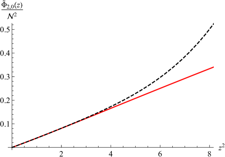
Figure 10: Taylor expansion to 8th order as given in Eq. (168)–(171) (dashed curve) of $\tilde{\Phi}_{2,0}(z)$ (red, solid line).

In order to calculate the asymptotics for large $z$ we consider $z^{2}{\textstyle\frac{\mathrm{d}}{\mathrm{d}z^{2}}}\tilde{\Phi}_{2,0}(z)$, which helps to solve the integrals but eliminates the constant part. Using again the variable transformations $x_{1}={\textstyle\frac{1}{x}}-1$, $x_{3}={\textstyle\frac{y}{x}}$, and $x_{2}={\textstyle\frac{y_{2}}{x}}$ the integral reads

$$z^{2}{\textstyle\frac{\mathrm{d}}{\mathrm{d}(z^{2})}}\tilde{\Phi}_{2,0}(z) ={{\cal N}^{2}}\int_{0}^{1}\mathrm{d}x\int_{0}^{\infty}\mathrm{d}y\int_{0}^{\infty}\mathrm{d}y_{2}\;\big{[}F_{z}^{(1)}(x,y,y_{2})+F_{z}^{(2)}(x,y,y_{2})\big{]}$$ (173)

$$F_{z}^{(1)}(x,y,y_{2}) =\frac{xz^{2}(1-x)}{(y+y_{2})^{2}(1+y+y_{2}+(1-x)xz^{2})}$$ (174)

$$F_{z}^{(2)}(x,y,y_{2}) =\frac{-xz^{2}[y(1-x+y_{2})+(1-x)y_{2}]}{(y+y_{2}+yy_{2})^{2}\big{[}(1+y+y_{2})(y+y_{2}+yy_{2})+xz^{2}(y_{2}-xy_{2}+y(1-x+y_{2}))\big{]}}$$ (175)

We distinguish the cases $y<1$ and $y>1$ and split $z^{2}{\textstyle\frac{\mathrm{d}}{\mathrm{d}z^{2}}}\tilde{\Phi}_{2,0}(z)=A_{<}+A_{>}$ accordingly. For $y<1$ the limit $z\to\infty$ exists and can be taken in the integrand. This integration gives a constant,

$$\lim_{z\to\infty}A_{<}=\int_{0}^{1}\mathrm{d}x\int_{0}^{\infty}\mathrm{d}y\int_{0}^{1}\mathrm{d}y_{2}\;\left[\frac{1}{(y+y_{2})^{2}}-\frac{1}{(y+y_{2}+yy_{2})^{2}}\right]=\ln 2\ .$$ (176)

For $y>1$ we perform the $y$ and $y_{2}$ integration over the first term in Eq. (167), then expand to lowest orders in $\frac{1}{z}$ and integrate over $x$. This gives the logarithm

$$\int_{0}^{1}\mathrm{d}x\int_{0}^{\infty}\mathrm{d}y\int_{0}^{\infty}\mathrm{d}y_{2}\;F_{z}^{(1)}(x,y,y_{2}) =-3+2\ln z+{\cal O}(z\ln z).$$ (177)

Obtaining the next order is more delicate than expanding in $\frac{1}{z}$ before the $x$-integration. The second term gives again only a constant, and the limit $z\to\infty$ can be taken in the integrand

$$\lim_{z\to\infty}\int_{0}^{1}\mathrm{d}x\int_{0}^{\infty}\mathrm{d}y\int_{0}^{\infty}\mathrm{d}y_{2}\;F_{z}^{(2)}(x,y,y_{2})=-\ln 2\ .$$ (178)

In summary, we find

$$z^{2}\frac{{\mathrm{d}}}{{\mathrm{d}}z^{2}}\tilde{\Phi}_{2,0}(z) ={{\cal N}^{2}}\big{[}2\ln z-3+{\cal O}({\textstyle\frac{1}{z}}\ln z)\big{]}\ .$$ (179)

And consequently after integration

$$\tilde{\Phi}_{2,0}(z) ={{\cal N}^{2}}\big{[}2(\ln z)^{2}-6\ln z+\alpha_{0}+{\cal O}({\textstyle\frac{1}{z}}\ln z)\big{]}.$$ (180)

We plot the asymptotics in Fig. 11 and find numerically $\alpha_{0}\approx 6.17(2)$.

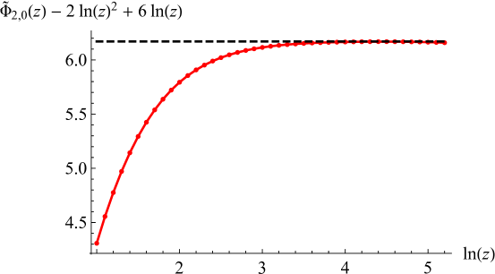
Figure 11: Asymptotics of $\tilde{\Phi}_{2,0}(z)-2\ln(z)^{2}+6\ln(z)$ for large $z$. The dashed line is the asypmptotic value $6.17$.

References

- [1] O. Narayan and D.S. Fisher, Threshold critical dynamics of driven interfaces in random media, Phys. Rev. B 48 (1993) 7030–42.
- [2] O. Narayan and D.S. Fisher, Critical behavior of sliding charge-density waves in 4-epsilon dimensions, Phys. Rev. B 46 (1992) 11520–49.
- [3] O. Narayan and D.S. Fisher, Dynamics of sliding charge-density waves in 4-epsilon dimensions, Phys. Rev. Lett. 68 (1992) 3615–18.
- [4] H. Leschhorn, T. Nattermann, S. Stepanow and L.-H. Tang, Driven interface depinning in a disordered medium, Annalen der Physik 509 (1997) 1–34, arXiv:cond-mat/9603114.
- [5] T. Nattermann, S. Stepanow, L.-H. Tang and H. Leschhorn, Dynamics of interface depinning in a disordered medium, J. Phys. II (France) 2 (1992) 1483–8.
- [6] P. Le Doussal, K.J. Wiese and P. Chauve, Functional renormalization group and the field theory of disordered elastic systems, Phys. Rev. E 69 (2004) 026112, cond-mat/0304614.
- [7] P. Le Doussal, K.J. Wiese and P. Chauve, 2-loop functional renormalization group analysis of the depinning transition, Phys. Rev. B 66 (2002) 174201, cond-mat/0205108.
- [8] P. Chauve, P. Le Doussal and K.J. Wiese, Renormalization of pinned elastic systems: How does it work beyond one loop?, Phys. Rev. Lett. 86 (2001) 1785–1788, cond-mat/0006056.
- [9] A.A. Middleton, P. Le Doussal and K.J. Wiese, Measuring functional renormalization group fixed-point functions for pinned manifolds, Phys. Rev. Lett. 98 (2007) 155701, cond-mat/0606160.
- [10] K.J. Wiese, C. Husemann and P. Le Doussal, Field theory of disordered elastic interfaces at 3-loop order: The -function, Nucl. Phys. B 932 (2018) 540-588, arXiv:1801.08483.
- [11] K. Johansson, Shape fluctuations and random matrices, Communications in Mathematical Physics 209 (2000) 437–76, math/9903134.
- [12] M. Prähofer and H. Spohn, Universal distributions for growth processes in 1 + 1 dimensions and random matrices, Phys. Rev. Lett. 84 (2000) 4882–4885, cond-mat/9912264.
- [13] M. Prähofer and H. Spohn, Statistical self-similarity of one-dimensional growth processes, Physica A 279 (2000) 342–52, cond-mat/9910273.
- [14] M. Kardar, G. Parisi and Y.-C. Zhang, Dynamic scaling of growing interfaces, Phys. Rev. Lett. 56 (1986) 889–892.
- [15] E. Frey and U.C. Täuber, Two-loop renormalization group analysis of the Burgers-Kardar-Parisi-Zhang equation, Phys. Rev. E 50 (1994) 1024–1045.
- [16] M. Lässig, On the renormalization of the Kardar-Parisi-Zhang equation, Nucl. Phys. B 448 (1995) 559–574, cond-mat/9501094.
- [17] E. Frey, U.C. Täuber and T. Hwa, Mode coupling and renormalization group results for the noisy Burgers equation, Phys. Rev. E 53 (1996) 4424.
- [18] K.J. Wiese, Critical discussion of the 2-loop calculations for the KPZ-equation, Phys. Rev. E 56 (1997) 5013–5017, cond-mat/9706009.
- [19] K.J. Wiese, On the perturbation expansion of the KPZ-equation, J. Stat. Phys. 93 (1998) 143–154, cond-mat/9802068.
- [20] E. Marinari, A. Pagnani and G. Parisi, Critical exponents of the KPZ equation via multi-surface coding numerical simulations, J. Phys. A 33 (2000) 8181–92.
- [21] M. Prähofer and H. Spohn, An exactly solved model of three-dimensional surface growth in the anisotropic KPZ regime, J. Stat. Phys. 88 (1997) 999–1012, cond-mat/9612209.
- [22] J. Krug, Origins of scale invariance in growth processes, Advances in Physics 46 (1997) 139–282.
- [23] M. Mezard, Disordered systems and Burger’s turbulence, J. Phys. IV (France) 8 (1997) 27–38, cond-mat/9801029.
- [24] E. Medina, T. Hwa, M. Kardar and Y.C. Zhang, Burgers equation with correlated noise: Renormalization-group analysis and applications to directed polymers and interface growth, Phys. Rev. A 39 (1989) 3053.
- [25] T. Hwa and D.S. Fisher, Anomalous fluctuations of directed polymers in random media, Phys. Rev. B 49 (1994) 3136–54, cond-mat/9309016.
- [26] R. Bundschuh and T. Hwa, An analytic study of the phase transition line in local sequence alignment with gaps, Discrete Applied Mathematics 104 (2000) 113–42.
- [27] R. Bundschuh and T. Hwa, RNA secondary structure formation: a solvable model of heteropolymer folding, Phys. Rev. Lett. 83 (1999) 1479–82, cond-mat/9903089.
- [28] T. Hwa and M. Lässig, Optimal detection of sequence similarity by local alignment. RECOMB 98, pages 109–16, 1998, cond-mat/9712081.
- [29] T. Nattermann, Theory of the random field Ising model, in A.P. Young, editor, Spin glasses and random fields, World Scientific, Singapore, 1997, cond-mat/9705295.
- [30] S. Lemerle, J. Ferré, C. Chappert, V. Mathet, T. Giamarchi and P. Le Doussal, Domain wall creep in an Ising ultrathin magnetic film, Phys. Rev. Lett. 80 (1998) 849.
- [31] G. Grüner, The dynamics of charge-density waves, Rev. Mod. Phys. 60 (1988) 1129–81.
- [32] G. Blatter, M.V. Feigel’man, V.B. Geshkenbein, A.I. Larkin and V.M. Vinokur, Vortices in high-temperature superconductors, Rev. Mod. Phys. 66 (1994) 1125.
- [33] T. Giamarchi and P. Le Doussal, Statics and dynamics of disordered elastic systems, in A.P. Young, editor, Spin glasses and random fields, World Scientific, Singapore, 1997, cond-mat/9705096.
- [34] T. Giamarchi and P. Le Doussal, Elastic theory of flux lattices in the presence of weak disorder, Phys. Rev. B 52 (1995) 1242–70, cond-mat/9501087.
- [35] T. Giamarchi and P. Le Doussal, Elastic theory of pinned flux lattices, Phys. Rev. Lett. 72 (1994) 1530–3.
- [36] T. Nattermann and S. Scheidl, Vortex-glass phases in type-II superconductors, Advances in Physics 49 (2000) 607–704, cond-mat/0003052.
- [37] P. Le Doussal, K.J. Wiese, S. Moulinet and E. Rolley, Height fluctuations of a contact line: A direct measurement of the renormalized disorder correlator, EPL 87 (2009) 56001, arXiv:0904.4156.
- [38] A. Prevost, E. Rolley and C. Guthmann, Dynamics of a helium-4 meniscus on a strongly disordered cesium substrate, Phys. Rev. B 65 (2002) 064517/1–8.
- [39] A. Prevost, PhD thesis, Orsay, 1999.
- [40] D. Ertas and M. Kardar, Critical dynamics of contact line depinning, Phys. Rev. E 49 (1994) 2532.
- [41] P. Le Doussal and K.J. Wiese, Elasticity of a contact-line and avalanche-size distribution at depinning, Phys. Rev. E 82 (2010) 011108, arXiv:0908.4001.
- [42] M. Kardar, Lectures on directed paths in random media, in F. David, P. Ginsparg and J. Zinn-Justin, editors, Fluctuating Geometries in Statistical Mechanics and Field Theory, Volume LXII of Les Houches, école d’été de physique théorique 1994, Elsevier Science, Amsterdam, 1996.
- [43] L.E. Aragon, A.B. Kolton, P. Le Doussal, K.J. Wiese and E. Jagla, Avalanches in tip-driven interfaces in random media, EPL 113 (2016) 10002, arXiv:1510.06795.
- [44] G. Durin, F. Bohn, M.A. Correa, R.L. Sommer, P. Le Doussal and K.J. Wiese, Quantitative scaling of magnetic avalanches, Phys. Rev. Lett. 117 (2016) 087201, arXiv:1601.01331.
- [45] L. Laurson, X. Illa, S. Santucci, K.T. Tallakstad, K.J. Måløy and M.J. Alava, Evolution of the average avalanche shape with the universality class, Nat. Commun. 4 (2013) 2927.
- [46] G. Durin and S. Zapperi, Scaling exponents for Barkhausen avalanches in polycrystalline and amorphous ferromagnets, Phys. Rev. Lett. 84 (2000) 4705–4708.
- [47] O. Perkovic, K. Dahmen and JP. Sethna, Avalanches, Barkhausen noise, and plain old criticality, Phys. Rev. Lett. 75 (1995) 4528–4531.
- [48] P. Le Doussal and K.J. Wiese, Avalanche dynamics of elastic interfaces, Phys. Rev. E 88 (2013) 022106, arXiv:1302.4316.
- [49] A. Dobrinevski, P. Le Doussal and K.J. Wiese, Statistics of avalanches with relaxation and Barkhausen noise: A solvable model, Phys. Rev. E 88 (2013) 032106, arXiv:1304.7219.
- [50] A. Dobrinevski, P. Le Doussal and K.J. Wiese, Non-stationary dynamics of the Alessandro-Beatrice-Bertotti-Montorsi model, Phys. Rev. E 85 (2012) 031105, arXiv:1112.6307.
- [51] P. Le Doussal, M. Müller and K.J. Wiese, Equilibrium avalanches in spin glasses, Phys. Rev. B 85 (2012) 214402, arXiv:1110.2011.
- [52] P. Le Doussal and K.J. Wiese, Driven particle in a random landscape: disorder correlator, avalanche distribution and extreme value statistics of records, Phys. Rev. E 79 (2009) 051105, arXiv:0808.3217.
- [53] Z. Zhu and K.J. Wiese, The spatial shape of avalanches, Phys. Rev. E 96 (2017) 062116, arXiv:1708.01078.
- [54] K.J. Wiese and A.A. Fedorenko, Field theories for loop-erased random walks, (2018), arXiv:1802.08830.
- [55] P. Le Doussal, Finite temperature Functional RG, droplets and decaying Burgers turbulence, Europhys. Lett. 76 (2006) 457–463, cond-mat/0605490.
- [56] P. Le Doussal and K.J. Wiese, How to measure Functional RG fixed-point functions for dynamics and at depinning, EPL 77 (2007) 66001, cond-mat/0610525.
- [57] A. Rosso, P. Le Doussal and K.J. Wiese, Numerical calculation of the functional renormalization group fixed-point functions at the depinning transition, Phys. Rev. B 75 (2007) 220201, cond-mat/0610821.
- [58] P. Le Doussal, M. Müller and K.J. Wiese, Cusps and shocks in the renormalized potential of glassy random manifolds: How functional renormalization group and replica symmetry breaking fit together, Phys. Rev. B 77 (2007) 064203, arXiv:0711.3929.
- [59] P. Le Doussal and K.J. Wiese, First-principle derivation of static avalanche-size distribution, Phys. Rev. E 85 (2011) 061102, arXiv:1111.3172.
- [60] P. Le Doussal, A.A. Middleton and K.J. Wiese, Statistics of static avalanches in a random pinning landscape, Phys. Rev. E 79 (2009) 050101 (R), arXiv:0803.1142.
- [61] P. Le Doussal and K.J. Wiese, Size distributions of shocks and static avalanches from the functional renormalization group, Phys. Rev. E 79 (2009) 051106, arXiv:0812.1893.
- [62] A. Rosso, P. Le Doussal and K.J. Wiese, Avalanche-size distribution at the depinning transition: A numerical test of the theory, Phys. Rev. B 80 (2009) 144204, arXiv:0904.1123.
- [63] M. Kardar, D.A. Huse, C.L. Henley and D.S. Fisher, Roughening by impurities at finite temperatures (comment and reply), Phys. Rev. Lett. 55 (1985) 2923–4.
- [64] A.A. Middleton, Numerical results for the ground-state interface in a random medium, Phys. Rev. E 52 (1995) R3337–40.
- [65] P. Le Doussal and C. Monthus, Exact solutions for the statistics of extrema of some random 1d landscapes, application to the equilibrium and the dynamics of the toy model, Physica A 317 (2003) 140–98, cond-mat/0204168.
- [66] P. Le Doussal and K.J. Wiese, Higher correlations, universal distributions and finite size scaling in the field theory of depinning, Phys. Rev. E 68 (2003) 046118, cond-mat/0301465.
- [67] P. Grassberger, D. Dhar and P. K. Mohanty, Oslo model, hyperuniformity, and the quenched Edwards-Wilkinson model, Phys. Rev. E 94 (2016) 042314.
- [68] E.E. Ferrero, S. Bustingorry and A.B. Kolton, Non-steady relaxation and critical exponents at the depinning transition, Phys. Rev. E 87 (2013) 032122, arXiv:1211.7275.
- [69] P. Le Doussal and K.J. Wiese, Functional renormalization group at large for random manifolds, Phys. Rev. Lett. 89 (2002) 125702, cond-mat/0109204.
- [70] P. Le Doussal and K.J. Wiese, Functional renormalization group at large for disordered elastic systems, and relation to replica symmetry breaking, Phys. Rev. B 68 (2003) 174202, cond-mat/0305634.
- [71] P. Le Doussal and K.J. Wiese, Derivation of the functional renormalization group -function at order for manifolds pinned by disorder, Nucl. Phys. B 701 (2004) 409–480, cond-mat/0406297.