New signals for vector-like down-type quark in $U(1)$ of $E_{6}$

Abstract

We consider the pair production of vector-like down-type quarks in an $E_{6}$ motivated model, where each of the produced down-type vector-like quark decays into an ordinary Standard Model light quark and a singlet scalar. Both the vector-like quark and singlet scalar appear naturally in the $E_{6}$ model with masses at the TeV scale with a favorable choice of symmetry breaking pattern. We focus on the non-standard decay of the vector-like quark and the new scalar which decays to two photons or two gluons. We analyze the signal for the vector-like quark production in the $2\gamma+\geq 2j$ channel and show how the scalar and vector-like quark masses can be determined at the Large Hadron Collider.

I Introduction

Elementary particle physics has been at crossroads of expecting a breakthrough to understanding what lies beyond the Standard Model (SM) for quite some time now. The Large Hadron Collider’s (LHC) discovery of the Higgs boson Chatrchyan:2012xdj ; Aad:2012tfa came much to the satisfaction of confirming the SM picture of electroweak interactions. Although the reported hints of several phenomena that would have definitely indicated of physics beyond the SM (BSM) have not survived further scrutiny by the LHC experiment, the diphoton excess at LHC CMS:2015dxe ; TheATLAScollaboration:2015mdt ; Aaboud:2016tru brought back the attention to heavy vector-like quarks and extended scalar sectors amongst many other models. The SM is widely believed to be an incomplete theory due to the lack of explanation to several outstanding issues (e.g. neutrino masses, dark matter candidate, etc.). The Grand Unified Theories (GUTs) are known to present novel ideas in addressing the above issues in the SM while also proposing to unify the three SM gauge couplings to one at a high scale. Most of the GUT models have testable consequences at the TeV scale which are in the form of an extra gauge group such as an extra $U(1)$ and some additional new particles with heavy masses. We look at such an example in the $E_{6}$ GUT model Gursey:1975ki where one gets down-type vector-like (VL) fermions charged under an extra $U(1)$ gauge symmetry. In this work we focus on an interesting signal of the down-type vector-like quark (VLQ) at LHC.

Note that vector-like fermions exist in many BSM scenarios and a lot of phenomenological studies on the down-type VLQs exist in the literatures delAguila:1998tp . The current experimental bounds on the mass of down-type VLQ are obtained under certain assumption of its decay modes Sirunyan:2017usq ; Sirunyan:2017ezy ; Aad:2015voa ; Khachatryan:2015gza ; Aad:2015kqa ; Aad:2015mba ; Aad:2011yn . For a down-type VLQ the searches are based on the assumption that it decays to one of the SM final states $Zb,Wt$ and $bh$. The current experimental lower bound on the mass of the down-type vector-like quark which mixes only with the third generation quark is around 730 GeV from Run 2 of the LHC Sirunyan:2017usq and is around 900 GeV from Run 1 of the LHC Khachatryan:2015gza . Similarly, the current lower bound for a vector-like quark which mixes with the light quarks is around 760 GeV from Run 1 of the LHC Aad:2011yn . While strong limits can be derived from these conventional search channels, the bounds get relaxed once new non-standard decay modes are present and start dominating over the SM channels. In this work we discuss a non-standard decay channel of the VLQ and about its possible signatures in a non supersymmetric version of $E_{6}$ model. A recent work discussing detailed phenomenology of vector-like quarks in $E_{6}$ model can be found in Ref. Joglekar:2016yap . In our case, we look at the VLQs and singlet scalars which are particles already present in the $E_{6}$ GUT, as discussed later. Using appropriate symmetry breaking pattern, one $U(1)$ in addition to the SM gauge symmetry remain unbroken at the TeV scale or even higher. The heavy down-type quark $xd$, which is a color triplet and an $SU(2)$ singlet with an electric charge of $-1/3$, is pair produced dominantly from two gluons via strong interactions at the LHC. Also, three such $xd$ and $\overline{xd}$ quarks naturally appear in our model based on $E_{6}$ from three fermion families. A singlet scalar is also naturally present which is responsible in breaking the additional $U(1)$ at the TeV scale. The pattern of symmetry breaking that we shall use gives the singlet scalar mass which is close to the $xd$-quark mass. Our $E_{6}$ model will be discussed in the next section. The quantum numbers of all the particles are fixed from the $E_{6}$ symmetry. The VLQ has a dominant decay mode in the non-standard form of a SM quark and the new singlet scalar which is the focus of this study. We discuss the phenomenology of such a scenario and on the observable signatures for the vector-like down-type quarks at the LHC when the singlet scalar decays to a pair of photons or a pair of gluons. We shall have events with dijet/diphoton resonances at the same mass and these predictions can be tested as more data accumulates at the upcoming 13 TeV LHC run.

This paper is organized as follows. In Section II below, we discuss our model and the formalism. In Section III, we discuss the phenomenology of our model. This gives emphasis on the prediction regarding the vector-like quarks through a new channel. The Section IV contains our conclusions and discussions.

II The model and formalism

We work with an effective symmetry at the TeV scale where the SM is augmented with an extra $U(1)^{\prime}$. This extra $U(1)^{\prime}$ is a special subgroup of the $E_{6}$ GUT gursey ; Langacker:2008yv ; general ; PLJW ; Erler:2002pr ; Kang:2004pp ; Kang:2004ix ; Kang:2009rd . We consider the non-supersymmetric version of $E_{6}$. The symmetry group $E_{6}$ is special in the sense that it is anomaly free, as well as has chiral fermions. Its fundamental representation decomposes under $SO(10)$ as

$$\bf 27=16+10+1~{}.$$

The representation 16 contains the $15$ SM fermions, as well as a right-handed neutrino. It decomposes under $SU(5)$ as

$$\bf 16=10+\bar{5}+1~{}.$$

And the 10 representation decomposes under $SU(5)$ as

$$\bf 10=5+\bar{5}+1~{}.$$

The 5 contains a color triplet and an $SU(2)_{L}$ doublet, whereas $\bf\bar{5}$ contains a color anti-triplet and another $SU(2)$ doublet, while the $\bf 1$ is a SM singlet. The gauge bosons are contained in the adjoint $\bf 78$ representation of $E_{6}$.

The full particle content of $\bf 27$ representation, which contains the SM fermions as well as extra fermions, are shown in the first two columns of Table 1. For three families of the SM fermions, we use three such $\bf 27$. The $E_{6}$ gauge symmetry can be broken as follows Group ; Hewett:1988xc

$$E_{6}\to\ SO(10)\times\ U(1)_{\psi}\to\ SU(5)\times\ U(1)_{\chi}\times\ U(1)_{\psi}~{}.~{}\,$$ (1)

The $U(1)_{\psi}$ and $U(1)_{\chi}$ charges for the $E_{6}$ fundamental ${\bf 27}$ representation are also given in Table 1. The $U(1)^{\prime}$ is a linear combination of the $U(1)_{\chi}$ and $U(1)_{\psi}$

$$Q^{\prime} = \cos\theta\ Q_{\chi}+\sin\theta\ Q_{\psi}~{}.~{}\,$$ (2)

The other orthogonal linear combination of $U(1)_{\chi}$ and $U(1)_{\psi}$ as well as the $SU(5)$ are broken at a high scale. This will allow us to have a large doublet-triplet splitting scale, which prevents rapid proton decay if the $E_{6}$ Yukawa relations were enforced. This will require either two pairs of (${\bf 27}$, ${\bf{\overline{27}}}$) and one pair of (${\bf 351^{\prime}}$, ${\bf\overline{351^{\prime}}}$) dimensional Higgs representations, or one pair of (${\bf 27}$, ${\bf{\overline{27}}}$), ${\bf 78}$, and one pair of (${\bf 351^{\prime}}$, ${\bf\overline{351^{\prime}}}$) dimensional Higgs representations (detailed studies of $E_{6}$ theories with broken Yukawa relations can be found in King:2005jy ; Babu:2015psa .) For our model, the unbroken symmetry at the TeV scale is $SU(3)_{C}\times SU(2)_{L}\times U(1)_{Y}\times U(1)^{\prime}$.

$SO(10)$	$SU(5)$	$2\sqrt{10}Q_{\chi}$	$2\sqrt{6}Q_{\psi}$	$4\sqrt{15}Q$
16	$10~{}(Q_{i},U_{i}^{c},E_{i}^{c})$	–1	1	$1$
	${\bar{5}}~{}(D_{i}^{c},L_{i})$	3	1	7
	$1~{}(N_{i}^{c}/T)$	–5	1	$-5$
10	$5~{}(XD_{i},XL_{i}^{c}/H_{u})$	2	–2	$-2$
	${\bar{5}}~{}(XD_{i}^{c},XL_{i}/H_{d})$	–2	–2	$-8$
1	$1~{}(XN_{i}/S)$	0	4	10

Table 1: Decomposition of the $E_{6}$ fundamental ${\bf 27}$ representation under $SO(10)$, $SU(5)$, and the $U(1)_{\chi}$, $U(1)_{\psi}$ and $U(1)^{\prime}$ charges.

We explain our convention in some details as given in Table 1. Our notation is similar to what is used in the supersymmetric case. We have denoted the SM quark doublets, right-handed up-type quarks, right-handed down-type quarks, lepton doublets, right-handed charged leptons, and right-handed neutrinos as $Q_{i}$, $U_{i}^{c}$, $D_{i}^{c}$, $L_{i}$, $E_{i}^{c}$, and $N_{i}^{c}$, respectively. In our model, we introduce three fermionic ${\bf 27}$s, one scalar Higgs doublet field $H_{u}$ from the doublet of ${\bf{5}}$ of $SU(5)$, one scalar Higgs doublet field $H_{d}$ from the doublet of ${\bf{\bar{5}}}$ of $SU(5)$, one scalar SM singlet Higgs field $T$ from the singlet of ${\bf 16}$ of $SO(10)$, and one scalar SM singlet Higgs field $S$ from the singlet of ${\bf 27}$ of $E_{6}$. Thus, similar to the fermions, all the scalars with masses at the TeV scale are coming from the ${\bf 27}$ of $E_{6}$. Note that the new additional fermions from the ${\bf 27}$ with masses at the TeV scale are $N_{i}^{c}$, $XD_{i}$, $XL_{i}^{c}$, $XD_{i}^{c}$, $XL_{i}$, and $XN_{i}$. For details see Table 2.

In our model, $S$ gives the Majorana masses to the right-handed neutrinos $N^{c}_{i}$ after $U(1)^{\prime}$ gauge symmetry breaking, i.e., the terms $SN_{i}^{c}N_{i}^{c}$ are $U(1)^{\prime}$ gauge invariant. Thus, the mixing angle in our model is given by

$$\tan\theta=\sqrt{5/3}~{}.~{}\,$$ (3)

$Q_{i}$	$(\mathbf{3},\mathbf{2},\mathbf{1/6},\mathbf{1})$	$U_{i}^{c}$	$(\mathbf{\overline{3}},\mathbf{1},\mathbf{-2/3},\mathbf{1})$	$D_{i}^{c}$	$(\mathbf{\overline{3}},\mathbf{1},\mathbf{1/3},\mathbf{7})$
$L_{i}$	$(\mathbf{1},\mathbf{2},\mathbf{-1/2},\mathbf{7})$	$E_{i}^{c}$	$(\mathbf{1},\mathbf{1},\mathbf{1},\mathbf{1})$	$N_{i}^{c}/T$	$(\mathbf{1},\mathbf{1},\mathbf{0},\mathbf{-5})$
$XD_{i}$	$(\mathbf{3},\mathbf{1},\mathbf{-1/3},\mathbf{-2})$	$XL^{c}_{i},~{}H_{u}$	$(\mathbf{1},\mathbf{2},\mathbf{1/2},\mathbf{-2})$	$XD_{i}^{c}$	$(\mathbf{\overline{3}},\mathbf{1},\mathbf{1/3},\mathbf{-8})$
$XL_{i},~{}H_{d}$	$(\mathbf{1},\mathbf{2},\mathbf{-1/2},\mathbf{-8})$	$XN_{i},~{}S$	$(\mathbf{1},\mathbf{1},\mathbf{0},\mathbf{10})$

Table 2: The particles and their quantum numbers under the $SU(3)_{C}\times SU(2)_{L}\times U(1)_{Y}\times U(1)^{\prime}$ gauge symmetry. Here, the correct $U(1)^{\prime}$ charges are the $U(1)^{\prime}$ charges in the above Table divided by $4{\sqrt{15}}$.

The Higgs potential needed for our purpose giving rise to the extra $U(1)$ symmetry breaking is

$$V=-m_{S}^{2}|S|^{2}-m_{T}^{2}|T|^{2}+\lambda_{S}|S|^{4}+\lambda_{T}|T|^{4}+\lambda_{ST}|S|^{2}|T|^{2}+(\sigma ST^{2}+H.C.)~{}.~{}\,$$ (4)

Among the parameters in the potential $V$, $\sigma$ is in general complex ($\sigma_{1}+i\sigma_{2}$) and all others are real. Note that without the term $\sigma ST^{2}$, there are two global $U(1)$ symmetries for the complex phases of $S$ and $T$. After $S$ and $T$ obtain the Vacuum Expectation Values (VEVs), we have two Goldstone bosons, and one of them is eaten by the extra $U(1)$ gauge boson. Thus, to avoid the extra Goldstone boson, one needs the term $\sigma ST^{2}$ to break one global symmetry. This leaves us with only one $U(1)$ symmetry in the above potential, which is the extra $U(1)^{\prime}$ gauge symmetry. Thus, after $S$ and $T$ acquire the VEVs, the $U(1)^{\prime}$ gauge symmetry is broken, and $S$ and $T$ will be mixed via the $\lambda_{ST}|S|^{2}|T|^{2}$ and $\sigma ST^{2}$ terms.

The SM gauge boson masses are determined by the VEVs of the $SU(2)$ doublet scalars and therefore $v_{EW}=\sqrt{v_{d}^{2}+v_{u}^{2}}\simeq 246$ GeV. The structure for the VEVs is given as

$$<H_{d}> =\begin{pmatrix}v_{d}/\sqrt{2}\\ 0\end{pmatrix}~{},~{} <H_{u}> =\begin{pmatrix}0\\ v_{u}/\sqrt{2}\end{pmatrix}~{},~{}$$ (5)

$$<T> =v_{t}/\sqrt{2}~{},~{} <S> =v_{s}/\sqrt{2}~{}~{}.$$ (6)

The mass squared matrices for the scalar sectors $(s_{1},t_{1})$ and $(s_{2},t_{2})$ are respectively given by

$$\mathcal{M}_{(s_{1},t_{1})}=\begin{pmatrix}2v_{s}^{2}\lambda_{S}-\frac{v_{t}^{2}\sigma_{1}}{\sqrt{2}v_{s}}&v_{t}(v_{s}\lambda_{ST}+\sqrt{2}\sigma_{1})\\ v_{t}(v_{s}\lambda_{ST}+\sqrt{2}\sigma_{1})&2v_{t}^{2}\lambda_{T}\end{pmatrix}\,\,\,\text{and}\,\,\,\mathcal{M}_{(s_{2},t_{2})}=\begin{pmatrix}-\frac{v_{t}^{2}\sigma_{1}}{\sqrt{2}v_{s}}&0\\ 0&0\end{pmatrix}.$$

$\sigma_{1}$ is the real part of $\sigma$ and the complex part $\sigma_{2}$ is assumed to be zero at tree level. These mass matrices have been obtained from the tree-level scalar potential under the assumption that there is no mixing in the $(S,T)$ and $(H_{u},H_{d})$ sector. The mass eigenstates for the CP-even sector $(s_{1},t_{1})$ is $s_{h}$ and $t_{h}$. The massive scalar from the CP-odd sector $(s_{2},t_{2})$ is represented by $a_{h}$. The relation between the gauge basis and the mass basis in for $(s_{1},t_{1})$ sector is given by

$$\begin{pmatrix}s_{1}\\ t_{1}\end{pmatrix}=\begin{pmatrix}\cos\alpha&\sin\alpha\\ -\sin\alpha&\cos\alpha\end{pmatrix}\begin{pmatrix}s_{h}\\ t_{h}\end{pmatrix},$$ (7)

where the mixing angle is given by

$$\sin 2\alpha=\frac{2m_{12}}{\sqrt{(m_{11}-m_{22})^{2}+4m_{12}^{2}}}$$

and

$$\cos 2\alpha=\frac{-(m_{11}-m_{22})}{\sqrt{(m_{11}-m_{22})^{2}+4m_{12}^{2}}},$$

while $m_{ij}$’s are different components of the matrix $\mathcal{M}_{(s1,t1)}$. For illustration for the given parameter values $(v_{s}=1.5\,\text{TeV},\lambda_{S}=1.78\times 10^{-4},\,\lambda_{T}=10^{-4},v_{t}=10^{5},\,\lambda_{ST}=1.86\times 10^{-2},\,\sigma_{1}=-9.8503\times 10^{-1})$, we get the masses of the scalars to be $m_{s_{h}}=600$ GeV, $m_{t_{h}}=2507$ GeV and $m_{a_{h}}=2155$ GeV. The value of $\sin\alpha$ for the above parameter set is 0.82.

The Yukawa couplings in our model are

$$-{\cal L} = y_{ij}^{U}Q_{i}U_{j}^{c}H_{u}+y_{ij}^{D}Q_{i}D_{j}^{c}H_{d}+y_{ij}^{E}L_{i}E_{j}^{c}H_{d}+y_{ij}^{N}L_{i}N_{j}^{c}H_{u}+y_{ij}^{XNd}XL_{i}^{c}XN_{j}H_{d}$$ (8)

$$+y_{ij}^{XNu}XL_{i}XN_{j}H_{u}+y_{ij}^{TD}D_{i}^{c}XD_{j}{T}+y_{ij}^{TL}XL_{i}^{c}L_{j}{T}$$

$$+y_{ij}^{SD}XD_{i}^{c}XD_{j}S+y_{ij}^{SL}XL_{i}^{c}XL_{j}S+{\rm H.C.}~{},~{}\,$$

where $i=1,~{}2,~{}3$. Thus, after $S$ and $T$ obtain VEVs or after $U(1)^{\prime}$ gauge symmetry breaking, $(XD_{i}^{c},~{}XD_{i})$ and $(XL_{i}^{c},~{}XL_{i})$ will become vector-like particles from the $y_{ij}^{SD}XD_{i}^{c}XD_{j}S$ and $y_{ij}^{SL}XL_{i}^{c}XL_{j}S$ terms, and $(D_{i}^{c},~{}XD_{i})$ and $(XL_{i}^{c},~{}L_{i})$ will obtain vector-like masses from the $y_{ij}^{TD}D_{i}^{c}XD_{j}{T}$ and $y_{ij}^{TL}XL_{i}^{c}L_{j}{T}$ terms. For simplicity, we assume $y_{ij}^{SD}\langle S\rangle>>y_{ij}^{TD}\langle{T}\rangle$ and $y_{ij}^{SL}\langle S\rangle>>y_{ij}^{TL}\langle{T}\rangle$. After we diagonalize their mass matrices, we obtain the mixings between $XD_{i}^{c}$ and $D_{i}^{c}$, and the mixings between $XL_{i}$ and $L_{i}$. The discussion of the Higgs potential for electroweak symmetry breaking is similar to the Type II two Higgs doublet model, so we will not repeat it here.

We note that the $U(1)^{\prime}$ gauge boson couples to all the SM fields in addition to the new matter and scalar fields. The covariant derivatives for the $SU(2)_{L}$ doublet and the singlet scalars are respectively given by

$$\begin{split}{\mathcal{D}}_{\mu}&=(\partial_{\mu}-i\frac{\vec{\sigma}}{2}.\vec{W_{\mu}}-ig^{\prime}YB_{\mu}-ig_{X}Y_{X}Z^{\prime}{{}_{\mu}}),\end{split}$$ (9)

where $Y(H_{u})=\frac{1}{2},Y(H_{d})=-\frac{1}{2}$ and $Y_{X}(H_{u})=-\frac{2}{4\sqrt{15}},Y_{X}(H_{d})=-\frac{8}{4\sqrt{15}}$;

$$\begin{split}{\mathcal{D}}_{\mu}&=(\partial_{\mu}-ig_{X}Y_{X}Z^{\prime}{{}_{\mu}}),\end{split}$$ (10)

where $Y_{X}(S)=\frac{10}{4\sqrt{15}}$ and $Y_{X}(T)=-\frac{5}{4\sqrt{15}}$. The mass square matrix for the neutral gauge boson sector in the $(W_{3},B,Z^{\prime})$ basis is then given as

$$\mathcal{M}=\begin{pmatrix}{\Huge({\mathcal{M}_{SM}})_{2\times 2}}&\begin{matrix}\mathcal{M}_{13}\\ \mathcal{M}_{23}\end{matrix}\\ \begin{matrix}\mathcal{M}_{13}&\mathcal{M}_{23}\end{matrix}&\mathcal{M}_{33}\end{pmatrix}~{},$$ (11)

where

$$\mathcal{M}_{13}=\frac{gg_{X}}{8\sqrt{15}}(2v_{u}^{2}-8v_{d}^{2}) \mathcal{M}_{23}=-\frac{g^{\prime}g_{X}}{8\sqrt{15}}(2v_{u}^{2}-8v_{d}^{2})~{},$$ ,

$${\rm and} \mathcal{M}_{33}=\frac{g_{X}^{2}}{240}(4v_{u}^{2}+64v_{d}^{2}+25v_{t}^{2}+100v_{s}^{2})~{}.$$ (12)

We can clearly see that the new gauge boson mass is dependent on the VEVs of all the scalars, such that one can choose one singlet VEV to be much smaller than the other and still have a very heavy $Z^{\prime}$ that evades the existing limits. Moreover, the mixings between $W_{3}/B$ and $Z^{\prime}$ will be zero at tree level if $v_{u}=2v_{d}$.

The mass matrix for the down-type quarks and the charged leptons in the $(q_{1},q_{2},q_{3},xq_{1},xq_{2},xq_{3})$ basis is given by

$$\frac{1}{\sqrt{2}}\begin{pmatrix}y_{ij}^{D}v_{d}&0\\ y_{ji}^{TD}v_{t}&y_{ij}^{SD}v_{s}\end{pmatrix}, \frac{1}{\sqrt{2}}\begin{pmatrix}y_{ij}^{E}v_{d}&y_{ji}^{TL}v_{t}\\ 0&y_{ij}^{SL}v_{s}\end{pmatrix},$$ (13)

where $i,j=1,2,3$. The $q_{i}$s and $xq_{i}$s represent the down-type quarks for the left matrix and charged leptons for the right matrix. These mass matrices would be diagonalized by a bi-unitary transformation which would lead to a mixing between the vector-like fermions and the SM fermions. However, one should note that the mixings between the left-handed fermions and the right-handed fermions will be dictated by different set of mixing angles. In our analysis we will allow mixings between the $d$ quark and the 1st generation vector-like quark($xd_{1}^{0}$) only and the mass matrix in the gauge basis $(d^{0},xd_{1}^{0})$ is given by

$$\frac{1}{\sqrt{2}}\begin{pmatrix}y_{11}^{D}v_{d}&0\\ y_{11}^{TD}v_{t}&y_{11}^{SD}v_{s}\end{pmatrix}\equiv\begin{pmatrix}m_{1}&0\\ m_{2}&m_{3}\end{pmatrix}.$$

The mixing matrices which transform the gauge eigenstates $(d^{0},xd_{1}^{0})$ to mass eigenstates$(d,xd_{1})$ are given by

$$S_{i}=\begin{pmatrix}\cos\theta_{i}&-\sin\theta_{i}\\ \sin\theta_{i}&\cos\theta_{i}\end{pmatrix},\text{where}\,\,\,i=L,R,$$ (14)

with the following left and right handed mixing angles

$$\sin 2\theta_{L}=\frac{2m_{1}m_{2}}{\sqrt{(m_{1}^{2}-m_{2}^{2}-m_{3}^{2})^{2}+4m_{1}^{2}m_{2}^{2}}},\,\,\,\,\,\,\,\,\, \cos 2\theta_{L}=\frac{-(m_{1}^{2}-m_{2}^{2}-m_{3}^{2})}{\sqrt{(m_{1}^{2}-m_{2}^{2}-m_{3}^{2})^{2}+4m_{1}^{2}m_{2}^{2}}},$$

$$\sin 2\theta_{R}=\frac{2m_{2}m_{3}}{\sqrt{(m_{1}^{2}+m_{2}^{2}-m_{3}^{2})^{2}+4m_{2}^{2}m_{3}^{2}}},\,\,\,\,\,\,\,\,\,\, \cos 2\theta_{R}=\frac{-(m_{1}^{2}+m_{2}^{2}-m_{3}^{2})}{\sqrt{(m_{1}^{2}+m_{2}^{2}-m_{3}^{2})^{2}+4m_{2}^{2}m_{3}^{2}}}.$$

We should also point out a few useful assumptions that we think are relevant for the analysis:

1. We have neglected any mixing between the electroweak doublet scalars and singlet scalars.

2. We also ensure that the new $U(1)^{\prime}$ gauge boson does not have a significant mixing with the SM gauge boson $Z$ ($\mathcal{M}_{13},\mathcal{M}_{23}<<\mathcal{M}_{33}$).

3. For simplicity, we will take all types of Yukawa couplings $y^{A}_{ij}$ to be zero for $i\neq j$, where $A\equiv TD,TL,SD,SL$ (see eq.8).

4. The mixing angles between the left-handed SM fermions and the vector-like fermions are taken to be very very small, i.e., we assume the left-mixing angle $\theta_{L}\sim 0$ to avoid the flavour physics constraints Alok:2014yua . For the choice of the set of parameter values {$\frac{y_{11}^{D}v_{d}}{\sqrt{2}}\sim m_{d}$, $\frac{y_{11}^{SD}v_{s}}{\sqrt{2}}\sim 640$ GeV, $v_{t}\sim 10^{4}$ GeV, $y_{11}^{TD}\sim 10^{-5}$} we get small values of mixing angles, i.e., $\sin\theta_{L}\sim 10^{-10}$ and $\sin\theta_{R}\sim 10^{-4}$.

III Signals for vector-like quarks

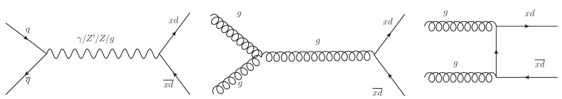
Figure 1: The leading-order Feynman diagrams for the subprocess contributing to the pair production of the VLQ at the LHC.

The new VLQ will be dominantly produced via strong interaction, with subleading contributions coming from the $s$-channel exchange of the $\gamma,Z$ and $Z^{\prime}$. In situations where the VLQ mass is less than $M_{Z^{\prime}}/2$, then the $Z^{\prime}$ mediated process can give a resonant contribution. However these contributions are found to be not very significant. We list the various production mechanisms of the VLQ in Fig.1. Note that one can in principle also produce the VLQs singly but they would be heavily suppressed as the production strength would depend on the mixing between the VLQs and SM quarks.

In Fig. 2 we show the pair production cross section of the VLQ $xd_{1}$ as a function of its mass at both run-1 and current run of the LHC with $\sqrt{s}=13$ TeV. With a few 100 femtobarns of cross section, it would be highly unlikely for the LHC to miss the signal for VLQs when they decay directly to SM particles. These already put strong limits on the mass of the VLQs. However, a new decay mode for the VLQ can definitely alter the search strategies for these exotics even when the rates are significantly high.

With the details of the model discussed in the previous section, it is now possible to write down the interaction vertices for the VLQ and new scalars with the SM particles that we use in our calculation and analysis. We list the relevant interactions in Table 3.

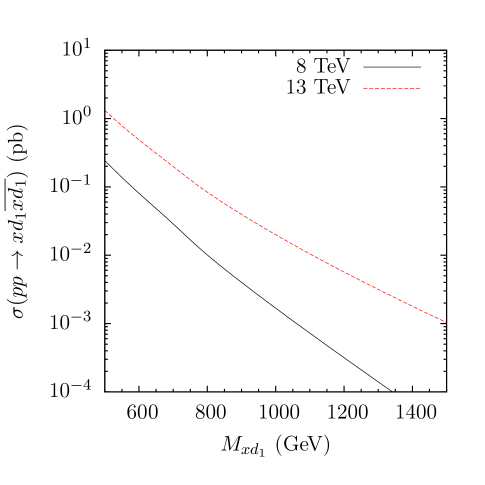
Figure 2: The pair production cross section of $xd_{1}$ at the LHC with $\sqrt{s}=13$ TeV as a function of $M_{xd_{1}}$.

	$K$	$c_{V}$	$c_{A}$
$\overline{d}\,d\,Z_{\mu}$	$\frac{e}{12\sin{2\theta_{w}}}$	$4\cos{2\theta_{w}}+3\cos{2\theta_{L}}-1$	$3(1+\cos{2\theta_{L}})$
$\overline{xd_{1}}\,xd_{1}\,Z_{\mu}$	$\frac{e}{12\sin{2\theta_{w}}}$	$4\cos{2\theta_{w}}-3\cos{2\theta_{L}}-1$	$3(1-\cos{2\theta_{L}})$
$\overline{d}\,xd_{1}\,Z_{\mu}$	$\frac{e}{4}\frac{\sin{2\theta_{L}}}{\sin{2\theta_{w}}}$	1	1
$\overline{u}\,d\,W^{+}$	$\frac{-e}{2\sqrt{2}}\frac{\cos{\theta_{L}}}{\sin{\theta_{w}}}V_{ud}$	1	1
$\overline{u}\,xd_{1}\,W^{+}$	$\frac{-e}{2\sqrt{2}}\frac{\sin{\theta_{L}}}{\sin{\theta_{w}}}V_{ud}$	1	1
$\overline{d}\,d\,Z^{\prime}_{\mu}$	$\frac{g_{X}}{16\sqrt{15}}$	$15\cos{2\theta_{R}}-3\cos{2\theta_{L}}$	$-(15\cos{2\theta_{R}}+3\cos{2\theta_{L}}-2)$
$\overline{xd_{1}}\,xd_{1}\,Z^{\prime}_{\mu}$	$-\frac{g_{X}}{16\sqrt{15}}$	$15\cos{2\theta_{R}}-3\cos{2\theta_{L}}$	$-(15\cos{2\theta_{R}}+3\cos{2\theta_{L}}+2)$
$\overline{d}\,xd_{1}\,Z^{\prime}_{\mu}$	$\frac{3g_{X}}{16\sqrt{15}}$	$5\sin{2\theta_{R}}-\sin{2\theta_{L}}$	$-(5\sin{2\theta_{R}}+\sin{2\theta_{L}})$
	$K$	$c_{S}$	$c_{P}$
$\overline{d}\,d\,s_{h}$	$-\frac{\sin{\theta_{L}}}{\sqrt{2}}$	$y_{11}^{SD}\cos{\alpha}\sin\theta_{R}+y_{11}^{TD}\sin\alpha\cos\theta_{R}$	0
$\overline{xd_{1}}\,xd_{1}\,s_{h}$	$\frac{-\cos\theta_{L}}{\sqrt{2}}$	$y_{11}^{SD}\cos{\alpha}\cos\theta_{R}-y_{11}^{TD}\sin\alpha\sin\theta_{R}$	0
		$y_{11}^{SD}\cos\alpha\sin(\theta_{L}+\theta_{R})$	$y_{11}^{SD}\cos\alpha\sin(\theta_{L}-\theta_{R})$
$\overline{d}\,xd_{1}\,s_{h}$	$\frac{1}{2\sqrt{2}}$	$+\,y_{11}^{TD}\sin\alpha\cos(\theta_{L}+\theta_{R})$	$-\,y_{11}^{TD}\sin\alpha\cos(\theta_{L}-\theta_{R})$
$\overline{d}\,d\,t_{h}$	$\frac{-\sin\theta_{L}}{\sqrt{2}}$	$y_{11}^{SD}\sin\alpha\sin\theta_{R}-y_{11}^{TD}\cos\alpha\cos\theta_{R}$	0
		$y_{11}^{SD}\sin\alpha\sin(\theta_{L}+\theta_{R})$	$y_{11}^{SD}\sin\alpha\sin(\theta_{L}-\theta_{R})$
$\overline{d}\,xd_{1}\,t_{h}$	$\frac{1}{2\sqrt{2}}$	$-\,y_{11}^{TD}\cos\alpha\cos(\theta_{L}+\theta_{R})$	$+\,y_{11}^{TD}\cos\alpha\cos(\theta_{L}-\theta_{R})$
$\overline{xd_{1}}\,xd_{1}\,t_{h}$	$\frac{-\cos\theta_{L}}{\sqrt{2}}$	$y_{11}^{SD}\sin\alpha\cos\theta_{R}\,+\,y_{11}^{TD}\cos\alpha\sin\theta_{R}$	0

Table 3: The couplings of VLQ $xd_{1}$ and $d$-quark with SM gauge bosons and, with the scalars $s_{h}$ and $t_{h}$. Coupling with gauge bosons are of the form $K\gamma^{\mu}(c_{V}-c_{A}\gamma^{5})$ and with scalars are of the form $K(c_{S}-c_{P}\gamma^{5})$. Here $\alpha$ is the scalar sector mixing angle in Eq. (7), $\theta_{L}$ and $\theta_{R}$ are left and right mixing angles in Eq. (14).

The possible decay modes for a down-type VLQ in our model are to the SM particles given by $xd_{1}\rightarrow h\,d,\,d\,Z,\,\text{and}\,u\,W^{-}$ while the non-standard decay modes would be $xd_{1}\rightarrow s_{h}\,d,\,t_{h}\,d,\,a_{h}\,d,\text{and}\,d\,Z^{\prime}$. Here $h$ is the SM Higgs boson, $u$ and $d$ are SM first generation quarks, $Z$ and $W^{-}$ are SM gauge bosons. $s_{h}$ and $t_{h}$ are CP-even scalars from $(S,T)$ sector while $a_{h}$ is CP-odd scalar from $(S,T)$ sector. For simplicity we focus on the case where out of all the SM down-type quarks, $xd_{1}$ interacts only with the $d$ quark through the Yukawa interaction with $S$ and $T$. For a very small mixing between $xd_{1}$ and $d$ quark and for a $Z^{\prime}$ heavier than $xd_{1}$, the dominant decay modes of $xd_{1}$ become $s_{h}\,d,\,\,t_{h}\,d$ and $a_{h}\,d$. The other decay modes are suppressed because the interaction strength for these decays are proportional to the very small mixing angles $\sin\theta_{L}$ and $\sin\theta_{R}$ (Table 3). As discussed in the previous section and to be safe from flavor constraints, one can impose small mixing angles, for example, $\sin\theta_{L}\sim 10^{-10}$ and $\sin\theta_{R}\sim 10^{-4}$ as mentioned for a set of parameter choices of the model. This will insure that the vector-like fermions do not decay to the SM gauge bosons and light SM fermions Grossmann:2010wm . The decay to the SM Higgs and light down-type quark is again very suppressed, due to the coupling strength being proportional to $\sin\theta_{R}$ and mass of the down-type SM quark. The mixing in the Higgs sector has been neglected as a convenient choice to keep the number of free parameters to tune to be small.

The $Z-Z^{\prime}$ mixing which is anyhow strongly constrained by electroweak data in any $U(1)$ extension beyond the SM is also negligible, thus avoiding the decay of VLQ to $d\,Z$ final state through this mixing. All other possible scalars other than $h$ from the doublet sector $(H_{u},\,H_{d})$ are heavier than the VLQ, and thus ensure absence of the decay of VLQ to them. So if both $a_{h}$ and $t_{h}$ are also heavier than $xd_{1}$, the VLQ $xd_{1}$ decays to the lone $s_{h}\,d$ final state. This decay is not suppressed due to a direct Yukawa coupling of the SM quark and VLQ with $T$ as well as the mixing between the $xd_{1}$ and $d$ in the right-handed sector. Thus, the decay is made possible through not only the mixing between the CP-even components of the scalars $S$ and $T$ but also depends on $\sin\theta_{R}$. It turns out that even with a choice of the Yukawa strength of $10^{-5}$ or lower (where $\sin\theta_{L}\sim 10^{-10}$ and $\sin\theta_{R}\sim 10^{-4}$), this decay is still the dominant channel. Thus, with the minimal assumptions that mixing of the new states with the SM sector being small and negligible allows a very specific decay channel for the VLQ in the model.

Once the VLQ is produced at the LHC, it will almost always decay into the non-standard channel to give a light quark jet and the scalar $s_{h}$. The $s_{h}$ then decays promptly to either SM particles or any lighter states of the new particles in the spectrum. The decay modes for the scalar can be summarized as $s_{h}\rightarrow\overline{\ell_{i}}\,\ell_{j},\overline{x\ell_{i}}\,x\ell_{j},\,\overline{x\ell_{i}}\,\ell_{j},\,\overline{\ell_{i}}\,x\ell_{j},\,\gamma\,\gamma,\,g\,g,\overline{d}\,d$. Here $\ell_{i}$s are SM charged leptons and $x\ell_{i}$s are vector-like leptons. We avoid the decay of $s_{h}$ to a pair of VLLs by setting their mass such that $M_{x\ell_{i}}>m_{s_{h}}/2$. Here $M_{x\ell_{i}}$ is mass for the $i^{th}$ generation vector-like lepton and $m_{s_{h}}$ is the mass of the scalar $s_{h}$. The Yukawa coupling $y_{ij}^{TL}$ has been chosen zero to avoid mixing between the VLL and the SM lepton sector, and thus avoiding the decay of $s_{h}$ to the final states $\overline{x\ell_{i}}\,\ell_{j}$, $\bar{\ell_{i}}\,x\ell_{j}$ and $\overline{\ell_{i}}\,\ell_{j}$. Additionally the decay to $\overline{d}d$ is controlled by the mixing angle $\sin\theta_{L}$ and is therefore too suppressed. With $xd_{1}$ heavier than $s_{h}$ the decay mode $s_{h}\rightarrow\overline{xd_{1}}\,d$ is not allowed. Hence the only allowed final states for $s_{h}$ decay are $\gamma\gamma$ and $gg$.

Decay to $\gamma\gamma$ and $gg$ will occur through the effective one-loop induced coupling. All of the three generations of down-type VLQs and charged VLLs will affect the branching ratios of $s_{h}$ to $\gamma\gamma$ and to $gg$. The coupling of $s_{h}$ to gluons and photons follows the standard notations that are being used in the literature and for clarification we are giving only the coupling with gluons by the effective Lagrangian

$$\mathcal{L}_{s_{h}GG}=-\lambda_{sgg}s_{h}~{}G_{\mu\nu}G^{\mu\nu}~{},$$ (15)

with the effective coupling $\lambda_{sgg}=\alpha_{s}F_{1/2}(\tau_{xd})/(16\pi v_{s})$ where

$$F_{1/2}(\tau_{xd})=2(\tau_{xd}+(\tau_{xd}-1)f(\tau_{xd}))\tau_{xd}^{-2}$$ (16)

represents the loop function and $f(\tau_{xd})=(sin^{-1}\sqrt{\tau_{xd}})^{2}$ with $\tau_{xd}=m_{s_{h}}^{2}/4M_{xd}^{2}\,\,<1$. Here, we have shown the contribution to the coupling from only one vector-like quark.

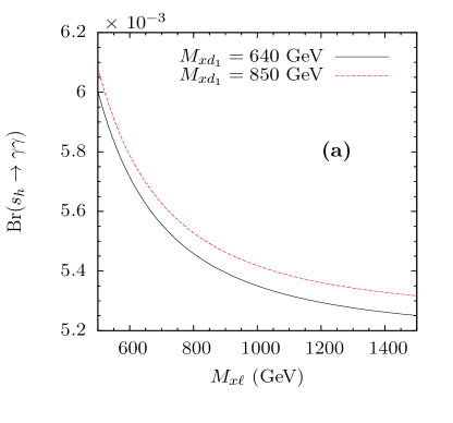
Figure 3: (a) Illustrating the diphoton branching ratio for $s_{h}$ decay as a function of the vector-like lepton mass for two different values of the lightest VLQ mass ($M_{xd_{1}}$). (b) The on-shell $s_{h}$ production cross section at LHC with $\sqrt{s}=13$ TeV through gluon-fusion as a function the singlet vev $v_{s}$ with $m_{s_{h}}=600$ GeV. For the above plots, we fix $M_{xd_{2}}\,=\,M_{xd_{3}}\,=$ 1.5 TeV, $y_{ii}^{SL}\,=\,1$. For (a) $M_{x\ell_{1}}\,=\,M_{x\ell_{2}}\,=\,M_{x\ell_{3}}\,=\,M_{x\ell}$, while for (b) $y_{11}^{SD}\,=\,1$, $M_{xd_{1}}=y_{11}^{SD}v_{s}/\sqrt{2}$, and $y_{22}^{SD}\,=\,\sqrt{2}\,M_{xd_{2}}/v_{s}$.

We plot the branching ratio for the scalar $s_{h}$ decaying into a pair of photons in Fig. 3 (a) as a function of the VLL masses for two values of the lightest VLQ mass($M_{xd_{1}}$), while the other two VLQs have masses at 1.5 TeV. As the mass of light vector-like leptons are not severely constrained by experiments, we shall consider the results with all the three VLLs contributing to the diphoton decay. Here the mass values of all the three vector-like leptons have been taken to be same ($M_{x\ell}$) while the Yukawa couplings of $s_{h}$ to VLLs have been taken to be unity ($y_{ii}^{SL}=1$).

Note that the branching of the $s_{h}\to\gamma\gamma$ is very similar to the order at which the SM Higgs decay happens but slightly higher. This is because of the contributions of the VLLs which do not contribute to the $s_{h}\to gg$ mode. However, the decay to $\gamma\gamma$ mode is still between 0.5% – 0.6% at best while the remaining decay probability is made up by the $gg$ channel.

Fig. 3 (b) shows the production cross section of a 600 GeV $s_{h}$ at $\sqrt{s}=13$ TeV center of mass energy as a function of the singlet vev $v_{s}$. The $s_{h}$ is being produced by the loop induced effective coupling in Eq. 15. For the cross section estimates we have chosen the Yukawa coupling of $s_{h}$ to the 1st generation VLQ $xd_{1}$ to be 1. The mass of $xd_{1}$ depends on the value $v_{s}$ following the relation $M_{xd_{1}}=y_{11}^{SD}v_{s}/\sqrt{2}$. The masses for the $xd_{2}$ and $xd_{3}$ have been taken to 1.5 TeV. The Yukawa couplings ($y_{22}^{SD}$ and $y_{33}^{SD}$) have different values for different values of $v_{s}$. Note that the $s_{h}$ production crucially depends on the Yukawa coupling which can be tuned to control its production rate. In fact, this possibility was earlier used by us Das:2015enc ; Das:2016xuc to arrive at the possible explanation of the now hitherto disproved diphoton excess for a 750 GeV resonance CMS:2015dxe ; TheATLAScollaboration:2015mdt ; Aaboud:2016tru .

As pointed out earlier, the VEVs for $S$ and $T$ which are given by $v_{s}$ and $v_{t}$ respectively play a significant role in giving mass to $Z^{\prime}$. We choose the mass of $Z^{\prime}$ to be 1.5 TeV which is still allowed by current LHC data, primarily due to the SM fermions carrying very suppressed quantum charges of the new $U(1)^{\prime}$ as shown in Table 2. As can be seen from the mass square matrix of the neutral gauge boson sector (Eq. (12)), by choosing large values of $v_{s}$ or $v_{t}$, it is possible to avoid mixing between the SM and new gauge boson sector. But the vector-like lepton masses are given by the relation, $M_{x\ell_{i}}=y_{ii}^{SL}v_{s}/\sqrt{2}$. And $y_{ii}^{SL}$ is the Yukawa coupling of $s_{h}$ to the VLLs which enters in the $s_{h}\gamma\gamma$ effective coupling. For a sub-TeV vector-like lepton and with significant value of Yukawa coupling it will not be possible to choose a very large value of $v_{s}$. We therefore choose a higher value for $v_{t}$ at 10 TeV which effectively suppresses any significant mixing in the neutral gauge boson sector.

Note that after the decay of the VLQs there will be two $s_{h}$ and two jets in the final state. As the $s_{h}$ decays to two gluons or to two photons only, with almost 99% to the gluonic jets, the resultant final states are either $2\gamma+4j$, $4\gamma+2j$ or $6j$. The cross section for the $4\gamma\,+\,2j$ final state is quite small while the QCD background for the $6j$ final state is significantly large compared to the $2\gamma\,+\,4j$ final state. Thus, these two channels would require large statistics to leave any imprint of their signal at the LHC. So in all likelihood the remaining channel of $2\gamma+4j$ seems the most promising channel which we shall focus on for our analysis.

For the $2\gamma+4j$ final state one of the $xd_{1}$ will eventually have a full hadronic decay to 3 jets. The bound on the branching ratio for the decay of a color triplet vector-like quark to three jets for different masses of vector-like quark has been obtained in Dobrescu:2016pda using the existing searches for resonances in multijet final states by the CDF Collaboration Aaltonen:2011sg at the Tevatron, and by the CMS and ATLAS Collaborations at the LHC using data from the 7 TeV ATLAS_CMS_7TeV , 8 TeV ATLAS_CMS_8TeV and 13 TeV ATLAS_13TeV runs. Ref. Dobrescu:2016pda shows that the physical region where BR(VLQ $\rightarrow 3j)\leq 1$ for different mass values of vector-like quark remains unconstrained except for a tiny region around 500 GeV.

	Model Parameters	Particle Mass	(Br($s_{h}\rightarrow\gamma\gamma$),  Br($s_{h}\rightarrow gg$))	$\sigma(pp\rightarrow xd_{1}\overline{xd_{1}})$
BP1	$\lambda_{T}=0.31$, $\lambda_{S}=0.088$, $\lambda_{ST}=0.75$, $v_{s}=950$ GeV, $v_{t}=10^{4}$ GeV, $\sigma_{1}=-83.96$ GeV, $\sin\alpha=0.71$	$M_{xd_{1}}=640$ GeV, $M_{x\ell_{i}}=500$ GeV, $m_{s_{h}}=600$ GeV, $m_{a_{h}}=2.5$ TeV, $m_{t_{h}}=3.5$ TeV	(0.006, 0.994)	339 fb
BP2	$\lambda_{T}=0.01$, $\lambda_{S}=0.269$, $\lambda_{ST}=0.216$, $v_{s}=2.5$ TeV, $v_{t}=10^{4}$ GeV, $\sigma_{1}=-141.4$ GeV, $\sin\alpha=0.9$	$M_{xd_{1}}=850$ GeV, $M_{x\ell_{i}}=500$ GeV, $m_{s_{h}}=600$ GeV, $m_{a_{h}}=2$ TeV, $m_{t_{h}}=3$ TeV	(0.006, 0.994)	56.4 fb

Table 4: Two benchmark scenarios. The cross section is evaluated at the 13 TeV LHC. Note that $y_{ii}^{SD}\,=\,\sqrt{2}\,M_{xd_{i}}/v_{s}$, $y_{ii}^{TD}\,=\,10^{-5}$ and we fix $M_{xd_{2}}=M_{xd_{3}}=1.5$ TeV.

To analyze the signal in our model, we note that the hardness of the jet from the decay $xd_{1}\rightarrow s_{h}\,j$ will depend on the mass difference between the VLQ $xd_{1}$ and the scalar $s_{h}$. This will affect the signal efficiency in the $2\gamma+4j$ channel as well as dictate how well the mass reconstruction for the parent particles can be made. We will discuss these features by considering two benchmark scenarios with different mass gaps between the $xd_{1}$ and $s_{h}$, where in one case the jet is hard while for the other case the jet would be comparatively soft. We choose BP1 ($M_{xd_{1}}=640$ GeV, $m_{s_{h}}=600$ GeV) with small mass difference between the VLQ and $s_{h}$ as well as BP2 ($M_{xd_{1}}=850$ GeV, $m_{s_{h}}=600$ GeV) with a large mass difference of $250$ GeV between them. For the two benchmarks the masses of the VLQs from the other two generations have been kept at 1.5 TeV. By comparing the cross sections for an 850 GeV VLQ with that of a 1.5 TeV VLQ from Fig. 2 it can be concluded that the two VLQs having mass of 1.5 TeV will not contribute to the final state of the analysis. Other benchmark details including the pair production cross section for $xd_{1}$ and the branching fractions for the decay of $s_{h}$ are shown in Table 4. We also check that the current upper limits on the cross section for the diphoton production through a narrow-width scalar resonance at 13 TeV run of LHC given by CMS Collaboration Khachatryan:2016yec is satisfied for our choice of the benchmark points. The upper limits on the cross section for the dijet production through a narrow-width resonance at the 13 TeV LHC, given by the CMS collaborationSirunyan:2016iap ; CMS_dijet_13TeV are also satisfied.

Note that for BP1 the mass difference between $xd_{1}$ and $s_{h}$ is 40 GeV. This would mean that the jet coming from the decay of $xd_{1}$ is quite soft. Although at a hadronic machine such as the LHC, the jet multiplicity from parton showering would be invariably increased, we intend to focus on relatively hard jets and therefore would like to neglect soft jets in the process. So for the analysis of BP1 we consider a final state with smaller jet multiplicity given by $2\gamma\,+\,\geq\,2j$. We demand that the jets have at least a minimum 40 GeV transverse momentum. The dominant SM background for such a final state is through all subprocesses contributing to $pp\rightarrow 2\gamma\,+\,\geq\,2j$ (with $p_{T}(j)\,>\,40$ GeV). For BP2 where the mass gap between $xd_{1}$ and $s_{h}$ is above 200 GeV, one expects the jet from $xd_{1}$ decay to be quite hard and thus the SM background is given by $pp\rightarrow 2\gamma\,+\,\geq\,4j$.

We have implemented the TeV-scale $U(1)^{\prime}$ extended model derived from $E_{6}$ GUT in LanHEP lanhep to generate the model files for CalcHEP Belyaev:2012qa . Using the model files we generated events for the pair production of VLQs (in LHEF format Alwall:2006yp ) at the LHC with $\sqrt{s}=13$ TeV and the subsequent decays of the $xd_{1}$ and $s_{h}$ were included as a decay table for the model (in SLHA formatslha ) with the help of CalcHEP. We then use these files to decay the unstable particles, and pass the generated parton-level events for showering and hadronization in PYTHIA 8.2 Sjostrand:2014zea . To enable detector simulation, we then linked the HepMC2 Dobbs:2001ck libraries with PYTHIA 8.2 to translate PYTHIA 8 events into HepMC format. For simulating the background, we generated the events at leading-order accuracy using MadGraph5 Alwall:2014hca . Pythia 6 Sjostrand:2006za interfaced in MadGraph5 was used for parton showering and hadronization of the background events, and to get event files in STDHEP format.

For both signal and background we include the detector effects and have reconstructed the final state objects using DELPHES 3 deFavereau:2013fsa . These are obtained in a CMS environment. Further, FastJet Cacciari:2011ma embedded in DELPHES has been used to reconstruct the jets. In the DELPHES framework the anti-$k_{T}$ algorithm with a cone size 0.5, $p_{T}^{j}>20$ GeV and $|\eta_{parton}|<2.5$ is used to reconstruct the jets. The phenomenological event-analysis is done with the MadAnalysis5 package using the event format ROOT.

In case of BP1 for which the mass difference between the lightest vector-like quark ($xd_{1}$) and the scalar ($s_{h}$) is small, we have generated $pp\rightarrow 2\gamma+2j$ events as background at 13 TeV LHC. At the level of generation of events certain basic cuts have been imposed on the final state particles. All jets and photons satisfy $|\eta|<2.5$ and each final state particle is separated from all other final state particles with an angular separation ($\Delta R$) value greater than 0.4. The transverse momenta of photons and jets satisfy

$$p_{T}(j)\,>\,20\,\,\text{GeV} p_{T}(\gamma)\,>\,100\,\,\text{GeV}.$$ and (17)

The final state photons for the signal come from the decay of the $s_{h}$ which has 600 GeV mass and hence the probability for the photons for the signal to have higher $p_{T}$ values is more compared to the background. Hence a 100 GeV $p_{T}$ cut for photon has been used for the generation of background because the phase space with lower photon $p_{T}$ will be largely populated by background compared to the signal. For 13 TeV LHC, with the above cuts taken into account and at leading-order (LO) accuracy the value of the cross section for the parton-level background for BP1 is around 234 fb.

For BP2 where the mass difference between $xd_{1}$ and $s_{h}$ is 250 GeV, $pp\rightarrow 2\gamma+4j$ events have been generated as the background. The basic cuts on the pseudo-rapidity ($\eta$) and on the angular separation ($\Delta R$) of the final state particles have been taken to be same as that of the benchmark BP1. The cut on the photon $p_{T}$ is taken to be the same 100 GeV as in case of BP1. We have imposed different $p_{T}$ cuts on the four jets and those are given by

$$p_{T}(j_{1})\,>\,80\,\,\text{GeV}, p_{T}(j_{2})\,>\,80\,\,\text{GeV}, p_{T}(j_{3})\,>\,40\,\,\text{GeV} p_{T}(j_{4})\,>\,40\,\,\text{GeV}.$$ and (18)

With the above cuts the cross section at the parton-level for the background, for BP2 i.e. for the process $pp\rightarrow 2\gamma+4j$, comes out to be around 12.15 fb. Similarly the signal events $pp\rightarrow xd_{1}xd_{1}$ have been generated using the event generator CalcHEP. The pair production cross sections are shown in Table 4. For the reconstructed events we choose the following selection criteria on the photons, jets and leptons

• A jet is considered in an event if $p_{T}(j)>40$ GeV and $|\eta(j)|<2.5$.

• An electron or a muon is considered in the lepton set if $p_{T}(\ell)>10$ GeV and $|\eta(\ell)|<2.5$.

• A photon is considered in an event if $p_{T}(\gamma)>40$ GeV and $|\eta(\gamma)|<2.5$.

• All final state candidates are separated from each other with a minimum angular separation satisfying $\Delta R>0.4$.

	No. of Events
Cuts	Signal	Background
Preselection	267	10626
$p_{T}(\gamma_{2})\geq 100$ GeV	248	9440
$p_{T}(j_{2})\geq 100$ GeV	210	2921
$p_{T}(\gamma_{1})\geq 200$ GeV	205	1735
$p_{T}(j_{1})\geq 150$ GeV	201	1534
$M_{eff}\geq 800$ GeV	201	1394

Table 5: The selected events after each step of selection criteria for BP1 with an integrated luminosity of 100 fb^-1.

	No. of Events
Cuts	Signal	Background
Preselection	40	685
$p_{T}(\gamma_{2})\geq 100$ GeV	37	634
$p_{T}(j_{2})\geq 100$ GeV	36	554
$p_{T}(\gamma_{1})\geq 200$ GeV	35	326
$M_{eff}\geq 1000$ GeV	35	293

Table 6: The selected events after each step of selection criteria for BP2 with an integrated luminosity of 100 fb^-1.

The preselection criteria for BP1 is to consider events having 2 photons and a minimum of two jets. For BP2 the preselection criteria is to consider events with two photons and a minimum of four jets in the final state. We vetoed all the events having at least one isolated lepton of $p_{T}$ value greater than 10 GeV. For the two leading (in $p_{T}$) jets and the two leading photons in the signal it is expected that they come from the decay of the VLQ. As the mass of the VLQ for the two cases is above 600 GeV, the two leading jets will have a large amount of $p_{T}$ compared to the leading jets in the background. So for both the benchmarks we have considered the events with the leading two jets and two photons with $p_{T}$ value greater than 100 GeV.

To further increase the signal-to-background ratio we apply the following selection cuts to the analysis for BP1

$$p_{T}(\gamma_{1})\geq 200\,\text{GeV}, p_{T}(j_{1})\geq 150\,\text{GeV}, M_{eff}\geq 800\,\text{GeV}.$$ (19)

The cut-flow table for BP1 signal and background is shown in Table 6. Note that to generate the background events with large statistics we have used the preselection cuts given in Eq. (17).

Similarly for BP2 we have besides the criterion in Eq. (17), the additional preselection requirements for jets as given by Eq. (18) to generate the SM background with good statistics. We further impose the stronger selection cuts on the events

$$p_{T}(\gamma_{1})\geq 200\,\text{GeV}, M_{eff}\geq 1000\,\text{GeV},$$ (20)

which help in improving the signal-to-background ratio for the signal events in the $2\gamma+4j$ final state.

With these cuts and a 100 fb^-1 integrated luminosity we get a statistical significance of 5$\sigma$ for BP1 as can be seen from the Table 6. For BP2 we get a significance of 1.9$\sigma$ as can be seen from Table 6. The significance is calculated using the formula $\sigma=\sqrt{\frac{S}{S+B}}$.

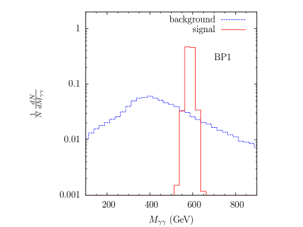
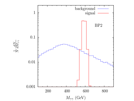
Figure 4: The normalized invariant mass distributions for the two leading photons of benchmark scenarios BP1 and BP2.

As we trigger upon two hard photons in the final state which come from the decay of the scalar $s_{h}$, the mass of the scalar $s_{h}$ can be reconstructed by looking at the invariant mass distribution of the two leading photons for both BP1 and BP2. To highlight this we plot the normalized invariant mass distribution of the two leading photons for both signal and background in Fig. 4. As expected the signal from the pair production of the VLQ is confined to a bin around the mass of the scalar $s_{h}$ with a clear peak for the signal at $m_{s_{h}}=600$ GeV. There would in principle also be an invariant mass peak for a jet pair around the $s_{h}$ mass which however is more challenging to observe due to the large spread in their invariant mass distribution.

Similarly, to reconstruct the mass of the VLQ one can use the fully hadronic channel giving three jets or the semi-hadronic channel giving two photons and a jet. With the knowledge of the reconstructed mass for $s_{h}$ through the $2\gamma$ invariant mass peak, the mass for the vector-like quark can be reconstructed for both BP1 and BP2. To compare the reconstruction of the VLQ in the two channels, we first plot the $3j$ invariant mass distribution comprised of the leading jets in the events for both the signal and background in Fig. 5. Although a distinct excess in the distribution exists around the mass of VLQ for both BP1 and BP2, the spread is quite wide and hence unclear as a mass resonance.

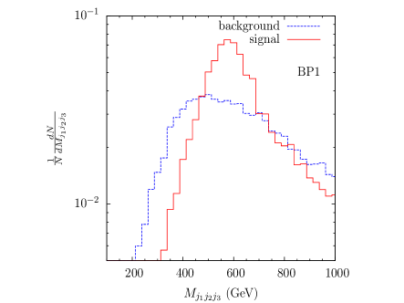
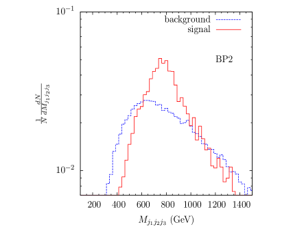
Figure 5: The invariant mass distribution for the leading three jets for both benchmark scenarios BP1 and BP2.

Although, the other channel with two photons and a hard jet should be a much more cleaner and precise mode to reconstruct the parent VLQ mass, it does suffer from the ambiguity of pairing the right jet with the pair of photons. In addition, for BP1 the mass splitting between the $xd_{1}$ and $s_{h}$ is quite small and therefore the choice of the right jet is affected by other soft jets that may originate from showering and fragmentation effects. To account for this ambiguity, we use the primary information on the kinematic characteristics of events for both BP1 and BP2 that is available to us to determine how we should combine the jets with the two photons. Owing to the small mass gap in BP1, we can safely assume that the two leading jets for the signal in BP1 would come from the decay of $s_{h}$ and therefore can be safely discounted in the combination. Of the remaining soft jets, all wrong combinations would only contribute in smearing the distribution for $M_{\gamma_{1}\gamma_{2}j}$. We therefore propose to neutralize the smearing effects by averaging over all such soft jets (with $p_{T}>40$ GeV) in the invariant mass

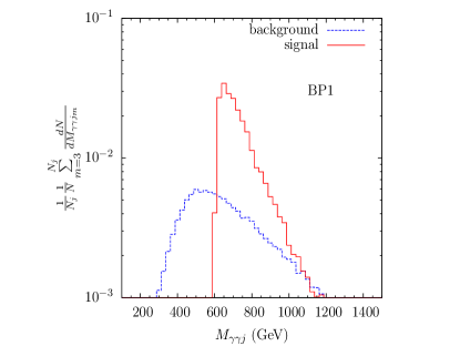
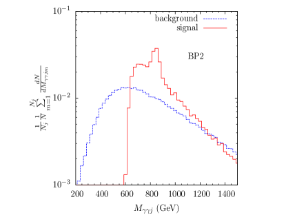
Figure 6: The average of normalized invariant mass distributions of the leading two photons with a jet. The average for BP1 starts from the third leading jet and the average for BP2 starts from the first leading jet.

reconstruction and neglecting the first two leading jets for BP1. For BP2, the jets coming from the decay of VLQ to $s_{h}j$ is equally hard as the ones that come from the decay of $s_{h}$ themselves. Therefore, for BP2, the averaging is done including all jets with $p_{T}>40$ GeV. We plot their normalized distribution after averaging for both signal and background in Fig. 6. As the diphoton coming from the $s_{h}$ decay marks a kinematic edge in the distribution, this can be clearly seen to happen at the mass value of $s_{h}$ at 600 GeV for both BP1 and BP2 which is absent for the invariant mass distribution in the $3j$ hadronic channel. In addition, a much cleaner and distinct peak can be observed for the VLQ mass for BP2. In case of BP1, as the VLQ mass at 640 GeV is quite close to the scalar $s_{h}$ mass of 600 GeV, resolving the VLQ (although visible) mass peak from the sharp kinematic edge is difficult. However, for a larger mass gap the peak should be distinctly identifiable as in BP2.

Finally to impress upon the fact that the VLQ mass can be clearly reconstructed through the modified invariant mass variable proposed above, we show the distribution without any normalization in Fig. 7 overlaying the signal for BP2 over the SM background. It clearly shows the VLQ mass peak over the background. Thus, we find that both the $s_{h}$ and $xd_{1}$ can be reconstructed clearly to determine their masses

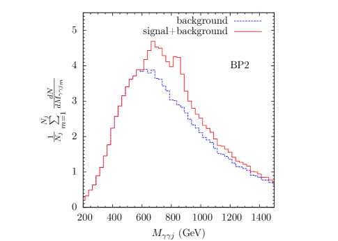
Figure 7: The average of invariant mass distributions of the leading two photons with a jet for BP2.

for the channel under study. As BP2 pertains to a VLQ mass of 850 GeV, we conclude that a TeV mass VLQ with such non-standard decay modes, possible for BSM scenarios which have very little mixing with the SM sector, can be observed and its mass parameters determined at the LHC with a few 100 fb^-1 of integrated luminosity.

IV Conclusion

In this work we have considered an $E_{6}$ motivated extension of the SM where the larger symmetry groups are broken at a very high scale and a residual $U(1)$ gauge symmetry is the only remaining symmetry beyond the unbroken SM gauge symmetry. This additional $U(1)$ then gets broken at the TeV scale through new SM singlet scalars giving rise to a TeV scale particle spectrum with three generations of vector-like quarks and leptons and several neutral scalars. The vector-like quarks in the model have non-standard decay modes and decay into an ordinary light quark and a SM singlet scalar. Further the scalar decays either to two photons or two gluons. The current experimental limits for VLQ which do not decay directly to the SM particles are very weak and therefore allow their mass to be as light as 500 GeV. We analyzed the events from such VLQ production at the LHC with $\sqrt{s}=13$ TeV in the $2\gamma+\geq 2j$ final states and present a search strategy for observing its signals. We also studied how to reconstruct the masses for both the scalar as well as the VLQ through a modified construction of the invariant mass variable using the $\gamma\gamma j$ sub-system. We saw that the mass of the scalar can be reconstructed from the invariant mass distribution of the two leading photons. With the upcoming high luminosity data at the LHC, the new signal for the VLQ, proposed in this work, could provide to be an interesting channel to search for new physics beyond the SM.

- (1) S. Chatrchyan et al. [CMS Collaboration], Phys. Lett. B 716, 30 (2012) doi:10.1016/j.physletb.2012.08.021 [arXiv:1207.7235 [hep-ex]].
- (2) G. Aad et al. [ATLAS Collaboration], Phys. Lett. B 716, 1 (2012) doi:10.1016/j.physletb.2012.08.020 [arXiv:1207.7214 [hep-ex]].
- (3) CMS Collaboration [CMS Collaboration], CMS-PAS-EXO-15-004.
- (4) The ATLAS collaboration, ATLAS-CONF-2015-081.
- (5) M. Aaboud et al. [ATLAS Collaboration], JHEP 1609, 001 (2016) doi:10.1007/JHEP09(2016)001 [arXiv:1606.03833 [hep-ex]].
- (6) F. Gursey, P. Ramond and P. Sikivie, Phys. Lett. 60B, 177 (1976). doi:10.1016/0370-2693(76)90417-2
- (7) F. del Aguila, J. A. Aguilar-Saavedra and R. Miquel, Phys. Rev. Lett. 82, 1628 (1999) doi:10.1103/PhysRevLett.82.1628 [hep-ph/9808400] ; S. Gopalakrishna, T. Mandal, S. Mitra and R. Tibrewala, Phys. Rev. D 84, 055001 (2011) doi:10.1103/PhysRevD.84.055001 [arXiv:1107.4306 [hep-ph]]; J. A. Aguilar-Saavedra, R. Benbrik, S. Heinemeyer and M. Pérez-Victoria, Phys. Rev. D 88, no. 9, 094010 (2013) doi:10.1103/PhysRevD.88.094010 [arXiv:1306.0572 [hep-ph]]; S. Gopalakrishna, T. Mandal, S. Mitra and G. Moreau, JHEP 1408, 079 (2014) doi:10.1007/JHEP08(2014)079 [arXiv:1306.2656 [hep-ph]]; C. Y. Chen, S. Dawson and Y. Zhang, Phys. Rev. D 92, no. 7, 075026 (2015) doi:10.1103/PhysRevD.92.075026 [arXiv:1507.07020 [hep-ph]]; F. del Aguila, M. Perez-Victoria and J. Santiago, JHEP 0009, 011 (2000) doi:10.1088/1126-6708/2000/09/011 [hep-ph/0007316]; A. Atre, M. Carena, T. Han and J. Santiago, Phys. Rev. D 79, 054018 (2009) doi:10.1103/PhysRevD.79.054018 [arXiv:0806.3966 [hep-ph]]; A. Atre, G. Azuelos, M. Carena, T. Han, E. Ozcan, J. Santiago and G. Unel, JHEP 1108, 080 (2011) doi:10.1007/JHEP08(2011)080 [arXiv:1102.1987 [hep-ph]]; R. Barcelo, A. Carmona, M. Chala, M. Masip and J. Santiago, Nucl. Phys. B 857, 172 (2012) doi:10.1016/j.nuclphysb.2011.12.012 [arXiv:1110.5914 [hep-ph]]; S. Fajfer, A. Greljo, J. F. Kamenik and I. Mustac, JHEP 1307, 155 (2013) doi:10.1007/JHEP07(2013)155 [arXiv:1304.4219 [hep-ph]]; J. P. Araque, N. F. Castro and J. Santiago, JHEP 1511, 120 (2015) doi:10.1007/JHEP11(2015)120 [arXiv:1507.05628 [hep-ph]]; M. Gillioz, R. Gröber, A. Kapuvari and M. Mühlleitner, JHEP 1403, 037 (2014) doi:10.1007/JHEP03(2014)037 [arXiv:1311.4453 [hep-ph]]; A. K. Alok and S. Gangal, Phys. Rev. D 86, 114009 (2012) doi:10.1103/PhysRevD.86.114009 [arXiv:1209.1987 [hep-ph]]; J. A. Aguilar-Saavedra, D. E. López-Fogliani and C. Muñoz, JHEP 1706, 095 (2017) doi:10.1007/JHEP06(2017)095 [arXiv:1705.02526 [hep-ph]]; G. Cacciapaglia, H. Cai, A. Carvalho, A. Deandrea, T. Flacke, B. Fuks, D. Majumder and H. S. Shao, JHEP 1707, no. 7, 005 (2017) doi:10.1007/JHEP07(2017)005 [arXiv:1703.10614 [hep-ph]]; C. H. Lee and R. N. Mohapatra, JHEP 1702, 080 (2017) doi:10.1007/JHEP02(2017)080 [arXiv:1611.05478 [hep-ph]]; B. Fuks and H. S. Shao, Eur. Phys. J. C 77, no. 2, 135 (2017) doi:10.1140/epjc/s10052-017-4686-z [arXiv:1610.04622 [hep-ph]]; F. J. Botella, G. C. Branco, M. Nebot, M. N. Rebelo and J. I. Silva-Marcos, Eur. Phys. J. C 77, no. 6, 408 (2017) doi:10.1140/epjc/s10052-017-4933-3 [arXiv:1610.03018 [hep-ph]]; A. Hebbar, G. K. Leontaris and Q. Shafi, Phys. Rev. D 93, no. 11, 111701 (2016) doi:10.1103/PhysRevD.93.111701 [arXiv:1604.08328 [hep-ph]]; S. Gopalakrishna and T. S. Mukherjee, arXiv:1702.04000 [hep-ph].
- (8) A. M. Sirunyan et al. [CMS Collaboration], arXiv:1706.03408 [hep-ex].
- (9) A. M. Sirunyan et al. [CMS Collaboration], JHEP 1705, 029 (2017) doi:10.1007/JHEP05(2017)029 [arXiv:1701.07409 [hep-ex]].
- (10) G. Aad et al. [ATLAS Collaboration], JHEP 1602, 110 (2016) doi:10.1007/JHEP02(2016)110 [arXiv:1510.02664 [hep-ex]].
- (11) V. Khachatryan et al. [CMS Collaboration], Phys. Rev. D 93, no. 11, 112009 (2016) doi:10.1103/PhysRevD.93.112009 [arXiv:1507.07129 [hep-ex]].
- (12) G. Aad et al. [ATLAS Collaboration], JHEP 1508, 105 (2015) doi:10.1007/JHEP08(2015)105 [arXiv:1505.04306 [hep-ex]].
- (13) G. Aad et al. [ATLAS Collaboration], Phys. Rev. D 91, no. 11, 112011 (2015) doi:10.1103/PhysRevD.91.112011 [arXiv:1503.05425 [hep-ex]].
- (14) G. Aad et al. [ATLAS Collaboration], Phys. Lett. B 712, 22 (2012) doi:10.1016/j.physletb.2012.03.082 [arXiv:1112.5755 [hep-ex]].
- (15) A. Joglekar and J. L. Rosner, arXiv:1607.06900 [hep-ph].
- (16) F. Gursey, P. Ramond P. Sikivie, Phys. Lett. 60B(1976)177; Y. Achiman and B. Stech, Phys. Lett. B(1978)389; Q. Shafi, Phys. Lett. 79B (1978)301; P. Ramond, Caltech Preprint CALT-68-709(1979).
- (17) For a review, see, P. Langacker, Rev. Mod. Phys. 81, 1199 (2009) [arXiv:0801.1345 [hep-ph]].
- (18) J. Erler, Nucl. Phys. B 586, 73 (2000).
- (19) P. Langacker and J. Wang, Phys. Rev. D 58, 115010 (1998).
- (20) J. Erler, P. Langacker and T. Li, Phys. Rev. D 66, 015002 (2002)
- (21) J. Kang, P. Langacker, T. Li and T. Liu, Phys. Rev. Lett. 94, 061801 (2005)
- (22) J. h. Kang, P. Langacker and T. Li, Phys. Rev. D 71, 015012 (2005)
- (23) J. Kang, P. Langacker, T. Li and T. Liu, JHEP 1104, 097 (2011)
- (24) R. Slansky, Phys. Rept. 79,1 (1981).
- (25) J. L. Hewett and T. G. Rizzo, Phys. Rept. 183, 193 (1989).
- (26) S. F. King, S. Moretti and R. Nevzorov, Phys. Rev. D 73, 035009 (2006); R. Howl and S. F. King, JHEP 0801, 030 (2008),
- (27) K. S. Babu, B. Bajc and V. Susič, JHEP 1505, 108 (2015).
- (28) A. Karozas, S. F. King, G. K. Leontaris and A. K. Meadowcroft, Phys. Lett. B 757, 73 (2016) [arXiv:1601.00640 [hep-ph]]; S. F. King and R. Nevzorov, JHEP 1603, 139 (2016) [arXiv:1601.07242 [hep-ph]].
- (29) B. N. Grossmann, B. McElrath, S. Nandi and S. K. Rai, Phys. Rev. D 82, 055021 (2010) [arXiv:1006.5019 [hep-ph]].
- (30) A. Belyaev, N. D. Christensen and A. Pukhov, Comput. Phys. Commun. 184, 1729 (2013) [arXiv:1207.6082 [hep-ph]].
- (31) A. K. Alok, S. Banerjee, D. Kumar and S. Uma Sankar, Nucl. Phys. B 906, 321 (2016) doi:10.1016/j.nuclphysb.2016.03.012 [arXiv:1402.1023 [hep-ph]].
- (32) K. Das and S. K. Rai, Phys. Rev. D 93, no. 9, 095007 (2016) doi:10.1103/PhysRevD.93.095007 [arXiv:1512.07789 [hep-ph]].
- (33) K. Das, T. Li, S. Nandi and S. K. Rai, arXiv:1607.00810 [hep-ph].
- (34) B. A. Dobrescu and F. Yu, arXiv:1612.01909 [hep-ph].
- (35) T. Aaltonen et al. [CDF Collaboration], Phys. Rev. Lett. 107, 042001 (2011) doi:10.1103/PhysRevLett.107.042001 [arXiv:1105.2815 [hep-ex]].
- (36) G. Aad et al. [ATLAS Collaboration], JHEP 1212, 086 (2012) doi:10.1007/JHEP12(2012)086 [arXiv:1210.4813 [hep-ex]]. S. Chatrchyan et al. [CMS Collaboration], Phys. Lett. B 718, 329 (2012) doi:10.1016/j.physletb.2012.10.048 [arXiv:1208.2931 [hep-ex]].
- (37) S. Chatrchyan et al. [CMS Collaboration], Phys. Lett. B 730, 193 (2014) doi:10.1016/j.physletb.2014.01.049 [arXiv:1311.1799 [hep-ex]]. G. Aad et al. [ATLAS Collaboration], Phys. Rev. D 91, no. 11, 112016 (2015) Erratum: [Phys. Rev. D 93, no. 3, 039901 (2016)] doi:10.1103/PhysRevD.93.039901, 10.1103/PhysRevD.91.112016 [arXiv:1502.05686 [hep-ex]].
- (38) ATLAS Collaboration, “Search for massive supersym-metric particles in multi-jet nal states produced in collisions at TeV,” note CONF-2016-057, Aug. 2016.
- (39) V. Khachatryan et al. [CMS Collaboration], Phys. Lett. B 767, 147 (2017) doi:10.1016/j.physletb.2017.01.027 [arXiv:1609.02507 [hep-ex]].
- (40) A. M. Sirunyan et al. [CMS Collaboration], Phys. Lett. B doi:10.1016/j.physletb.2017.02.012 [arXiv:1611.03568 [hep-ex]].
- (41) CMS Collaboration, “Search for dijet resonances in collisions at TeV using data collected in 2016,” Analysis Summary, CMS-PAS-EXO-16-056, March 2017.
- (42) A. Semenov, Comput. Phys. Commun. 180, 431 (2009) [arXiv:0805.0555 [hep-ph]]; A. Semenov, Comput. Phys. Commun. 201, 167 (2016) [arXiv:1412.5016 [physics.comp-ph]].
- (43) A. Belyaev, N. D. Christensen and A. Pukhov, Comput. Phys. Commun. 184, 1729 (2013) [arXiv:1207.6082 [hep-ph]].
- (44) J. Alwall et al., Comput. Phys. Commun. 176, 300 (2007) doi:10.1016/j.cpc.2006.11.010 [hep-ph/0609017].
- (45) P. Z. Skands et al., JHEP 0407, 036 (2004) doi:10.1088/1126-6708/2004/07/036 [hep-ph/0311123]. N. Desai and P. Z. Skands, Eur. Phys. J. C 72, 2238 (2012) doi:10.1140/epjc/s10052-012-2238-0 [arXiv:1109.5852 [hep-ph]].
- (46) T. Sjöstrand et al., Comput. Phys. Commun. 191, 159 (2015) doi:10.1016/j.cpc.2015.01.024 [arXiv:1410.3012 [hep-ph]].
- (47) M. Dobbs and J. B. Hansen, Comput. Phys. Commun. 134, 41 (2001). doi:10.1016/S0010-4655(00)00189-2
- (48) J. Alwall et al., JHEP 1407, 079 (2014) doi:10.1007/JHEP07(2014)079 [arXiv:1405.0301 [hep-ph]].
- (49) T. Sjostrand, S. Mrenna and P. Z. Skands, JHEP 0605, 026 (2006) doi:10.1088/1126-6708/2006/05/026 [hep-ph/0603175].
- (50) J. de Favereau et al. [DELPHES 3 Collaboration], JHEP 1402, 057 (2014) doi:10.1007/JHEP02(2014)057 [arXiv:1307.6346 [hep-ex]].
- (51) M. Cacciari, G. P. Salam and G. Soyez, Eur. Phys. J. C 72, 1896 (2012) doi:10.1140/epjc/s10052-012-1896-2 [arXiv:1111.6097 [hep-ph]].