Vacuum solutions around spherically symmetric and static objects
in the Starobinsky model

Abstract

The vacuum solutions around a spherically symmetric and static object in the Starobinsky model are studied with a perturbative approach. The differential equations for the components of the metric and the Ricci scalar are obtained and solved by using the method of matched asymptotic expansions. The presence of higher order terms in this gravity model leads to the formation of a boundary layer near the surface of the star allowing the accommodation of the extra boundary conditions on the Ricci scalar. Accordingly, the metric can be different from the Schwarzschild solution near the star depending on the value of the Ricci scalar at the surface of the star while matching the Schwarzschild metric far from the star.

I Introduction

A commonly followed path for addressing the accelerated expansion of the Universe is to modify Einstein’s general relativity (GR). One approach to modify GR is to replace the Einstein-Hilbert Lagrangian with a function of the Ricci scalar, the so-called $f\left(\mathcal{R}\right)$ models Sotiriou and Faraoni (2010); de Felice and Tsujikawa (2010); Capozziello and de Laurentis (2011); Nojiri and Odintsov (2011). Among these, the Starobinsky model Starobinsky (1980), $f\left(\mathcal{R}\right)=\mathcal{R}+\alpha\mathcal{R}^{2}$, is one of the most popular models of gravity as it provides a natural inflationary era in the early universe and it does not contain ghostlike modes.

The structures of relativistic stars have been studied to test $f\left(\mathcal{R}\right)$ models in a strong gravity regime in Refs. Kobayashi and Maeda (2009); Babichev and Langlois (2009, 2010); Jaime et al. (2011); Cooney et al. (2010); Arapoğlu et al. (2011); Ganguly et al. (2014); Arapoğlu et al. (2017); Yazadjiev et al. (2014); Staykov et al. (2014); Yazadjiev et al. (2015); Yazadjiev and Doneva (2015); Astashenok et al. (2013, 2014, 2015a, 2015b); Capozziello et al. (2016). The second term in the Lagrangian is assumed to be perturbative in Refs. Cooney et al. (2010); Arapoğlu et al. (2011), and the authors reduced the order by the method of perturbative constraints Eliezer and Woodard (1989); Jaén et al. (1986). More recently, another perturbative method known as matched asymptotic expansions (MAE) Bender and Orszag (1978); Holmes (2012) has been employed Ganguly et al. (2014); Arapoğlu et al. (2017) for the singular perturbation problem posed by the hydrostatic equations.

The latter approach requires extra boundary conditions since the order of the differential equations increases. The most reasonable choice for the extra boundary condition is the value of the Ricci scalar at the surface of the star. Yet, in $f\left(\mathcal{R}\right)$ theories, the vacuum solutions are not unique around a spherically symmetric and static object unlike the case in GR.

The vacuum solutions for $f(R)$ theories are studied by employing different approaches in Refs. Multamäki and Vilja (2006); Capozziello et al. (2007); Pun et al. (2008); Gao and Shen (2016). In these works, the authors search for a vacuum solution within $f\left(\mathcal{R}\right)$ models for specific choices of the Ricci scalar. Although they show that the Schwarzschild solution can be a vacuum solution for $f\left(\mathcal{R}\right)=\mathcal{R}+\alpha\mathcal{R}^{2}$, their results are not unique in the sense that different solutions of the field equations are also possible. Besides these works, the exterior solution is found as the Schwarzschild-de Sitter metric with a perturbative approach for $f\left(\mathcal{R}\right)$ models where the modified term is a power of the Ricci scalar in Ref. Cooney et al. (2010). A regular perturbative approach where the solutions are expanded as corrections to general relativity’s solutions is employed in this work although the trace equation poses a singular perturbation problem. Accordingly, some solutions might have been missed. A different perturbative approach is employed in Aparicio Resco et al. (2016), and the vacuum solutions are found as a decaying harmonic function of the Ricci scalar within $\mathcal{R}+\alpha\mathcal{R}^{2}$ for negative $\alpha$ values. Yet, negative $\alpha$ is known to lead to “ghosts” in the theory.

The no-hair theorem which states that a black hole is characterized by only its mass, spin, and electric charge Israel (1967, 1968); Carter (1971), is known to prevail in modified gravity theories Hawking (1972); Mayo and Bekenstein (1996); Psaltis et al. (2008); Sotiriou and Faraoni (2012); Cañate et al. (2016). The validity of the no-hair theorem is shown in Ref. Cañate et al. (2016) for the Starobinsky model with a spherically symmetric and static setup. Also, the authors of Ref. Mignemi and Wiltshire (1992) showed that the only static spherically symmetric asymptotically flat solution with a regular horizon is the Schwarzschild solution for positive values of $\alpha$.

In this work, the MAE method, which is appropriate for handling the singular perturbation problem Bender and Orszag (1978); Holmes (2012) posed by the trace equation, is employed to obtain the vacuum solutions around spherically symmetric objects. The results demonstrate the possibility of solutions other than the Schwarzschild solution in the $f\left(\mathcal{R}\right)=\mathcal{R}+\alpha\mathcal{R}^{2}$ gravity model around relativistic stars. Our results are applied to spherically symmetric and static black holes for vanishing Ricci scalar at the horizon and for this value our solutions reduce to the Schwarzschild metric, in full consistency with these previous results Mayo and Bekenstein (1996); Psaltis et al. (2008); Sotiriou and Faraoni (2012); Cañate et al. (2016); Mignemi and Wiltshire (1992).

The plan of the paper is as follows: The field equations are obtained in Sec. II. In Sec. III, these equations are solved by using the MAE method. Then, the composite solutions are constructed by matching these solutions, and the vacuum solution is obtained in the Starobinsky model in  Sec. IV. Finally, the vacuum solutions are discussed in Sec. V.

II Field Equations

The action of the Starobinsky model is

$$S=\frac{1}{16\pi}\int{\rm d}^{4}x\sqrt{-g}\left(\mathcal{R}+\alpha\mathcal{R}^{2}\right)+S_{\rm matter},$$ (1)

where $g$ is the determinant of the metric $g_{\mu\nu}$, $\mathcal{R}$ is the Ricci scalar, $\alpha$ is a positive constant, and $S_{\rm matter}$ is the action of matter. We assume the second term of the Lagrangian is a perturbative correction to the first term Jaén et al. (1986); Eliezer and Woodard (1989). In the metric formalism, the variation of the action with respect to the metric gives the field equations,

$$\left(1+2\alpha\mathcal{R}\right)G_{\mu\nu}+\frac{1}{2}\alpha g_{\mu\nu}\mathcal{R}^{2}-2\alpha\left(\nabla_{\mu}\nabla_{\nu}-g_{\mu\nu}\square\right)\mathcal{R}=8\pi T_{\mu\nu}$$ (2)

Sotiriou and Faraoni (2010); de Felice and Tsujikawa (2010). Contracting with the inverse metric, the trace equation is

$$6\alpha\square\mathcal{R}-\mathcal{R}=8\pi T.$$ (3)

A general form of the spherically symmetric and static metric is

$${\rm d}s^{2}=-h\left(r\right){\rm d}t^{2}+f\left(r\right){\rm d}r^{2}+r^{2}\left({\rm d}\theta^{2}+\sin^{2}\theta{\rm d}\phi^{2}\right).$$ (4)

All components of the energy-momentum tensor are zero in vacuum. Accordingly, by using the field equations and the trace equation, a set of differential equations for the metric components and the Ricci scalar in vacuum can be obtained as

$$6r \left(1+2\alpha\mathcal{R}\right)\left(1+2\alpha\mathcal{R}+\alpha r\mathcal{R}^{\prime}\right){\frac{{\rm d}f}{\mathrm{d}r}}$$

$$= f\left(1+2\alpha\mathcal{R}\right)\left[6\left(1+2\alpha\mathcal{R}\right)\left(1-f\right)+{r}^{2}f\mathcal{R}\left(2+3\alpha\mathcal{R}\right)\right]$$

$$+2\alpha f\left[6r\left(1+2{\alpha}\mathcal{R}\right)\left(1-f\right)+r^{3}f\mathcal{R}\left(1+3\alpha\mathcal{R}\right)\right]\mathcal{R}^{\prime}$$

$$+24{\alpha}^{2}f{r}^{2}\mathcal{R}^{\prime 2},$$ (5)

$$- \left(1+2\alpha\mathcal{R}+\alpha r\mathcal{R}^{\prime}\right)\frac{{\rm d}h}{\mathrm{d}r}$$

$$=\frac{h}{r}\left[1-f+\alpha\left(\frac{r^{2}f\mathcal{R}^{2}}{2}+2\left(1-f\right)\mathcal{R}+4r\mathcal{R}^{\prime}\right)\right],$$ (6)

$$6\alpha \left(1+2\alpha\mathcal{R}\right)r\frac{{\rm d}^{2}\mathcal{R}}{{\rm d}r^{2}}$$

$$= rf\mathcal{R}\left(1+2\alpha\mathcal{R}\right)-\alpha\mathcal{R}^{\prime}\left[6\left(1+2\alpha\mathcal{R}\right)\left(1+f\right)\right.$$

$$\left.-\left(1+3\alpha\mathcal{R}\right)r^{2}f\mathcal{R}\right]+12{\alpha}^{2}r\mathcal{R}^{\prime 2}.$$ (7)

Considering the third equation, this set of differential equations poses a singular perturbation problem Bender and Orszag (1978); Holmes (2012), since $\alpha$ is a small parameter. To solve these equations, we will use the MAE method which is appropriate for such problems. According to the MAE method, a boundary layer occurs where the highest derivative term is non-negligible compared with the other terms. The location of the boundary layer is not known from the beginning. Moreover, there could be more than one boundary layer. Instead of trying to locate the boundary layer, we work on a fictitious finite size domain where the boundary layer occurs at one of the edges of the region. Later, we will check which choices give physical solutions and construct the vacuum solutions accordingly. We use $R_{-}$ and $R_{+}$ to denote the nearest and the farthest points of the region to the star, respectively. To employ the MAE method, parameters should be nondimensionalized. With the definitions

$$x\equiv\frac{r}{L}-L_{\ast},\qquad L\equiv R_{+}-R_{-},\qquad L_{\ast}\equiv\frac{R_{-}}{L},$$ (8)

the problem is restricted to the interval $0<x<1$, and this leads to

$$r=\left(x+L_{\ast}\right)L,\qquad\frac{{\rm d}}{{\rm d}r}=\frac{1}{L}\frac{{\rm d}}{{\rm d}x},\qquad\frac{{\rm d}^{2}}{{\rm d}r^{2}}=\frac{1}{L^{2}}\frac{{\rm d}^{2}}{{\rm d}x^{2}}.$$ (9)

The other parameters can be made dimensionless by using finite scale factor $L$ as

$$\mathcal{\bar{R}}=L^{2}\mathcal{R},\qquad\epsilon=\frac{\alpha}{L^{2}}.$$ (10)

Then Eqs. (5), (6), and (7), respectively, become

$$\big{(}1+ 2\epsilon\mathcal{\bar{R}}+\epsilon\left(x+L_{\ast}\right)\mathcal{\bar{R}}^{\prime}\big{)}\frac{\mathrm{d}f}{\mathrm{d}x}$$

$$= \frac{f}{6}\left[6\left(1+2\epsilon\mathcal{\bar{R}}\right)\frac{1-f}{x+L_{\ast}}+{\left(x+L_{\ast}\right)}f\mathcal{\bar{R}}\left(2+3\epsilon\mathcal{\bar{R}}\right)\right]$$

$$+2\epsilon f\left[1-f+\left(x+L_{\ast}\right)^{2}\frac{f}{6}\frac{\left(1+3\epsilon\mathcal{\bar{R}}\right)}{\left(1+2\epsilon\mathcal{\bar{R}}\right)}\mathcal{\bar{R}}\right]\mathcal{\bar{R}}^{\prime}$$

$$+4\epsilon^{2}\left(x+L_{\ast}\right)\frac{f}{1+2\epsilon\mathcal{\bar{R}}}\mathcal{\bar{R}}^{\prime 2},$$ (11)

$$\big{(}1+ 2\epsilon\mathcal{\bar{R}}+\epsilon\left(x+L_{\ast}\right)\mathcal{\bar{R}}^{\prime}\big{)}\frac{{\rm d}h}{{\rm d}x}$$

$$= -\frac{h}{x+L_{\ast}}\left[1-f+\epsilon\left(\frac{\left(x+L_{\ast}\right)^{2}f\mathcal{\bar{R}}^{2}}{2}\right.\right.$$

$$+2\left(1-f\right)\mathcal{\bar{R}}+4\left(x+L_{\ast}\right)\mathcal{\bar{R}}^{\prime}\Bigg{)}\Bigg{]},$$ (12)

$$6\epsilon\big{(}1 +2\epsilon\mathcal{\bar{R}}\big{)}\left(x+L_{\ast}\right)\frac{\mathrm{d}^{2}\mathcal{\bar{R}}}{\mathrm{d}{x}^{2}}$$

$$= \left(x+L_{\ast}\right)f\mathcal{\bar{R}}\left(1+2\epsilon\mathcal{\bar{R}}\right)-\epsilon\mathcal{\bar{R}}^{\prime}\left[6\left(1+2\epsilon\mathcal{\bar{R}}\right)\left(1+f\right)\right.$$

$$\left.-\left(1+3\epsilon\mathcal{\bar{R}}\right)\left(x+L_{\ast}\right)^{2}f\mathcal{\bar{R}}\right]+12\epsilon^{2}\left(x+L_{\ast}\right)\mathcal{\bar{R}}^{\prime 2}.$$ (13)

Far from the object the metric should converge to the Minkowski metric. Therefore, the most reasonable boundary conditions for the components of the metric are $f\left(r\rightarrow\infty\right)=1$ and $h\left(r\rightarrow\infty\right)=1$, and for the Ricci scalar it is $\mathcal{R}\left(r\rightarrow\infty\right)=0$. The Starobinsky model is an exceptional case, among $f(\mathcal{R})$ theories, in that the Ricci scalar can be discontinuous at the surface of the object in the presence of thin shells or braneworlds Senovilla (2013). As we assume absences of braneworlds and thin shells in this paper, the interior of the star continuously matches with the exterior without any need for the Chameleon mechanism. This requires the continuity of the Ricci scalar and its derivative on the surface of the star according to junction conditions derived in Senovilla (2013). So, we choose the final boundary condition as $\mathcal{R}\left(r=R_{\ast}\right)=\mathcal{R}_{\ast}$ where $R_{\ast}$ is the radius of the star and $\mathcal{R}_{\ast}$ is the Ricci scalar at the surface of the star which is provided by the interior solutions of the star. The condition of continuity of Ricci scalar’s derivative can be used to test the validity of the solutions.

III Inner and Outer Solutions

According to the method, we need to seek solutions inside and outside the boundary layer separately. The solutions valid inside the boundary layer are called the inner solutions, and the solutions valid outside the boundary layer are called the outer solutions. Both of the solutions are introduced as perturbative series. The composite solutions, which are valid all over the interval of the problem, are constructed by combining the inner and outer solutions after matching them Bender and Orszag (1978); Holmes (2012).

III.1 Outer solutions

We can obtain the general outer solutions before deciding the location of the boundary layer. By introducing the outer solution of the Ricci scalar as a perturbative series,

$$\mathcal{\bar{R}}^{\rm out}\left(x\right)=\mathcal{\bar{R}}^{\rm out}_{0}\left(x\right)+\epsilon\mathcal{\bar{R}}^{\rm out}_{1}\left(x\right)+O\left(\epsilon^{2}\right),$$ (14)

Eq. (13) can be written up to the first order as

$$6\epsilon \left(x+L_{\ast}\right){\frac{\mathrm{d}^{2}\mathcal{\bar{R}}^{\rm out}_{0}}{\mathrm{d}{x}^{2}}}$$

$$= \left(x+L_{\ast}\right)f^{\rm out}\mathcal{\bar{R}}^{\rm out}_{0}+\epsilon\left(x+L_{\ast}\right)f^{\rm out}\left[\mathcal{\bar{R}}^{\rm out}_{1}+2\left(\mathcal{\bar{R}}^{{\rm out}}_{0}\right)^{2}\right]$$

$$-\epsilon\mathcal{\bar{R}}^{\rm out\prime}_{0}\left(6+6f^{\rm out}-\left(x+L_{\ast}\right)^{2}f^{\rm out}\mathcal{\bar{R}}^{\rm out}_{0}\right).$$ (15)

By solving the equation order by order, the solutions, independent from the boundary conditions, are obtained as

$$\mathcal{\bar{R}}^{\rm out}_{0}=\mathcal{\bar{R}}^{\rm out}_{1}=0,$$ (16)

since $f^{\rm out}\left(x\right)=0$ is not physical. Therefore, Eqs. (11) and (12) become

$$\frac{\mathrm{d}f^{\rm out}}{\mathrm{d}x}= \frac{f^{\rm out}}{x+L_{\ast}}\left(1-f^{\rm out}\right),$$ (17)

$$\frac{\mathrm{d}h^{\rm out}}{\mathrm{d}x}= -\frac{h^{\rm out}}{x+L_{\ast}}\left(1-f^{\rm out}\right).$$ (18)

These equations do not contain a perturbative part and they are similar to the GR case. The general solutions of these equations are

$$f^{\rm out}\left(x\right)= \frac{L_{\ast}+x}{A+x},$$ (19)

$$h^{\rm out}\left(x\right)= B\frac{A+x}{L_{\ast}+x}.$$ (20)

III.2 Inner solutions

We do not have any mathematical justification for the location of the boundary layer. Yet, the Ricci scalar is zero outside the boundary layer as found in the previous section. Then, a boundary layer which occurs at the farthest point of the fictitious region requires deviation of the Ricci scalar from zero with the divergence of the metric components from one (see Appendix A). That corresponds to a solution in which gravity increases radially away from the source in the vacuum which is not physical. So, a boundary layer can occur only at the nearest point of the fictitious region.

In a regular perturbative approach, due to the factor of $\epsilon$, the highest order differential term does not appear in the differential equations, and some solutions are missed because of this order reduction. According to the MAE method, the boundary layer is where the highest order differential term becomes non-negligible, and to appropriately examine solutions inside the boundary layer we need to define a new coordinate variable (coordinate stretching parameter)

$$\xi\equiv\frac{x}{\epsilon^{n}}.$$ (21)

With this definition, the derivative, ${\rm d}/{\rm d}x$, reduces the order of the term upon which it acts, as $n$. Hence, the highest order differential term becomes more significant.

In terms of the inner variable, Eq. (13) turns into

$$6\left(1+2\epsilon\mathcal{\bar{R}}^{\rm in}\right)\left(\epsilon^{1-n}\xi+\epsilon^{1-2n}L_{\ast}\right)\frac{{\rm d}^{2}\mathcal{\bar{R}}^{\rm in}}{{\rm d}\xi^{2}}= \left(\epsilon^{n}\xi+L_{\ast}\right)\left(1+2\epsilon\mathcal{\bar{R}}^{\rm in}\right)f^{\rm in}\mathcal{\bar{R}}^{\rm in}-\left[6\epsilon^{1-n}\left(1+f^{\rm in}\right)+12\epsilon^{2-n}\left(1+f^{\rm in}\right)\mathcal{\bar{R}}^{\rm in}\right]\left(\mathcal{\bar{R}}^{\rm in}\right)^{\prime}$$

$$+f^{\rm in}\left[\epsilon^{1+n}\xi^{2}\mathcal{\bar{R}}^{\rm in}+2\epsilon\xi L_{\ast}\mathcal{\bar{R}}^{\rm in}+{\epsilon}^{1-n}L_{\ast}^{2}\mathcal{\bar{R}}^{\rm in}+3\epsilon^{2+n}{\xi}^{2}\left(\mathcal{\bar{R}}^{\rm in}\right)^{2}\right]\left(\mathcal{\bar{R}}^{\rm in}\right)^{\prime}$$

$$+f^{\rm in}\left[6\epsilon^{2}\xi L_{\ast}\left(\mathcal{\bar{R}}^{\rm in}\right)^{2}+3\epsilon^{2-n}L_{\ast}^{2}\left(\mathcal{\bar{R}}^{\rm in}\right)^{2}\right]\left(\mathcal{\bar{R}}^{\rm in}\right)^{\prime}$$

$$+12\left(\epsilon^{2-n}\xi+\epsilon^{2-2n}L_{\ast}\right)\left(\mathcal{\bar{R}}^{\rm in}\right)^{\prime 2}.$$ (22)

$n$ should be chosen such that the highest order differential term and one of the other terms become the lowest order terms in the equation. Hence, the order reduction does not occur and no solutions are missed. Accordingly, $n=1/2$ is the most suitable choice to balance the second order differential term in the left-hand side of the equation with another term in the equation. Hence, the above equation becomes

$$6(1+2\epsilon\mathcal{\bar{R}}^{\rm in})(\sqrt{\epsilon}\xi+L_{\ast})\frac{{\rm d}^{2}\mathcal{\bar{R}}^{\rm in}}{{\rm d}\xi^{2}}= \left(\sqrt{\epsilon}\xi+L_{\ast}\right)\left(1+2\epsilon\mathcal{\bar{R}}^{\rm in}\right)f^{\rm in}\mathcal{\bar{R}}^{\rm in}-6\sqrt{\epsilon}\left(1+f^{\rm in}\right)\left(1+2\epsilon\mathcal{\bar{R}}^{\rm in}\right)\left(\mathcal{\bar{R}}^{\rm in}\right)^{\prime}$$

$$+(\epsilon^{3/2}\xi^{2}+2\epsilon\xi L_{\ast}+\sqrt{\epsilon}L_{\ast}^{2})(1+3\epsilon\mathcal{\bar{R}}^{\rm in})f^{\rm in}\mathcal{\bar{R}}^{\rm in}(\mathcal{\bar{R}}^{\rm in})^{\prime}+12(\epsilon^{3/2}\xi+\epsilon L_{\ast})(\mathcal{\bar{R}}^{\rm in})^{\prime 2}.$$ (23)

Similarly, Eqs. (11) and (12) become

$$\left[1+2\epsilon\mathcal{\bar{R}}^{\rm in}+\sqrt{\epsilon}\left(\xi\sqrt{\epsilon}+L_{\ast}\right)\left(\mathcal{\bar{R}}^{\rm in}\right)^{\prime}\right]{\frac{{\rm d}f^{\rm in}}{{\rm d}\xi}}= \frac{\sqrt{\epsilon}f^{\rm in}}{\xi\sqrt{\epsilon}+L_{\ast}}\left(1+2\epsilon\mathcal{\bar{R}}^{\rm in}\right)\left(1-f^{\rm in}\right)+\frac{\sqrt{\epsilon}}{6}f^{\rm in}\left(\xi\sqrt{\epsilon}+L_{\ast}\right)\left(2+3\epsilon\mathcal{\bar{R}}^{\rm in}\right)f^{\rm in}\mathcal{\bar{R}}^{\rm in}$$

$$+2\epsilon f^{\rm in}\left(\mathcal{\bar{R}}^{\rm in}\right)^{\prime}\left(1-f^{\rm in}\right)+\epsilon\frac{\left(f^{\rm in}\right)^{2}\left(\mathcal{\bar{R}}^{\rm in}\right)^{\prime}}{3\left(1+2\epsilon\mathcal{\bar{R}}^{\rm in}\right)}\left(\xi\sqrt{\epsilon}+L_{\ast}\right)^{2}\left(1+3\epsilon\mathcal{\bar{R}}^{\rm in}\right)\mathcal{\bar{R}}^{\rm in}$$

$$+4\epsilon^{3/2}f^{\rm in}\left(\xi\sqrt{\epsilon}+L_{\ast}\right)\frac{\left(\mathcal{\bar{R}}^{\rm in}\right)^{\prime 2}}{\left(1+2\epsilon\mathcal{\bar{R}}^{\rm in}\right)},$$ (24)

and

$$\frac{{\rm d}h^{\rm in}}{{\rm d}\xi}= -\frac{h^{\rm in}}{\left(\xi\sqrt{\epsilon}+L_{\ast}\right)\left(1+2\epsilon\mathcal{\bar{R}}^{\rm in}+\sqrt{\epsilon}\left(\xi\sqrt{\epsilon}+L_{\ast}\right)\left(\mathcal{\bar{R}}^{\rm in}\right)^{\prime}\right)}$$ (25)

$$\left\{\sqrt{\epsilon}\left(1-f^{\rm in}\right)+\epsilon\left[\frac{\sqrt{\epsilon}}{2}\left(\xi\sqrt{\epsilon}+L_{\ast}\right)^{2}f^{\rm in}\left(\mathcal{\bar{R}}^{\rm in}\right)^{2}+2\sqrt{\epsilon}\left(1-f^{\rm in}\right)\mathcal{\bar{R}}^{\rm in}+4\left(\xi\,\sqrt{\epsilon}+L_{\ast}\right)\left(\mathcal{\bar{R}}^{\rm in}\right)^{\prime}\right]\right\}.$$

The inner solutions are introduced as perturbed series,

$$f^{\rm in}\left(\xi\right)= f^{\rm in}_{0}\left(\xi\right)+\sqrt{\epsilon}f^{\rm in}_{1}\left(\xi\right)+\epsilon f^{\rm in}_{2}\left(\xi\right)+O\left(\epsilon^{3/2}\right),$$ (26)

$$h^{\rm in}\left(\xi\right)= h^{\rm in}_{0}\left(\xi\right)+\sqrt{\epsilon}h^{\rm in}_{1}\left(\xi\right)+\epsilon h^{\rm in}_{2}\left(\xi\right)+O\left(\epsilon^{3/2}\right),$$ (27)

$$\mathcal{R}^{\rm in}\left(\xi\right)= \mathcal{R}^{\rm in}_{0}\left(\xi\right)+\sqrt{\alpha}\mathcal{R}^{\rm in}_{1}\left(\xi\right)+\epsilon\mathcal{R}^{\rm in}_{2}\left(\xi\right)+O\left(\epsilon^{3/2}\right).$$ (28)

After plugging these solutions into Eqs. (24), (25), (23), they are found as

$$f_{0}^{\rm in}\left(\xi\right)= C_{0},$$ (29)

$$f_{1}^{\rm in}\left(\xi\right)= -\sqrt{\frac{2C_{0}^{3}}{3}}H_{0}L_{\ast}\exp\left(-\sqrt{\frac{C_{0}}{6}}\xi\right)+C_{0}\frac{1-C_{0}}{L_{\ast}}\xi+C_{1},$$ (30)

$$f_{2}^{\rm in}\left(\xi\right)= \left[\frac{H_{0}C_{0}^{2}}{12}\left(1-C_{0}\right)\xi^{2}-\frac{7\sqrt{6}C_{0}^{3/2}H_{0}}{12}\left(1-C_{0}\right)\xi+\frac{L_{\ast}}{6}C_{0}C_{1}H_{0}\xi\right]\exp\left(-\sqrt{\frac{C_{0}}{6}}\xi\right)$$

$$+\left[\frac{C_{0}H_{0}}{4}\left(1-5C_{0}\right)-\frac{5L_{\ast}C_{1}H_{0}}{12}\sqrt{6C_{0}}-\frac{1}{3}L_{\ast}\sqrt{6}C_{0}^{3/2}H_{1}\right]\exp\left(-\sqrt{\frac{C_{0}}{6}}\xi\right)$$

$$+\frac{5}{6}L_{\ast}^{2}H_{0}^{2}C_{0}^{2}\exp\left(-2\sqrt{\frac{C_{0}}{6}}\xi\right)+\frac{C_{0}^{2}}{L_{\ast}^{2}}\left(C_{0}-1\right)\xi^{2}+\frac{C_{1}}{L_{\ast}}\left(1-2C_{0}\right)\xi+C_{2},$$ (31)

$$h_{0}^{\rm in}\left(\xi\right)= D_{0},$$ (32)

$$h_{1}^{\rm in}\left(\xi\right)= D_{0}\frac{C_{0}-1}{L_{\ast}}\xi+D_{1},$$ (33)

$$h_{2}^{\rm in}\left(\xi\right)= \left(C_{0}-3\right)D_{0}H_{0}\exp\left(-\sqrt{\frac{C_{0}}{6}}\xi\right)+\frac{D_{1}\left(C_{0}-1\right)+C_{1}D_{0}}{L_{\ast}}\xi+\frac{D_{0}}{L_{\ast}^{2}}\left(1-C_{0}\right)\xi^{2}+D_{2},$$ (34)

$$\mathcal{\bar{R}}_{0}^{\rm in}\left(\xi\right)= H_{0}\exp\left(-\sqrt{\frac{C_{0}}{6}}\xi\right),$$ (35)

$$\mathcal{\bar{R}}_{1}^{\rm in}\left(\xi\right)= H_{1}\exp\left(-\sqrt{\frac{C_{0}}{6}}\xi\right)-\frac{H_{0}}{24L_{\ast}C_{0}}\left[\sqrt{6C_{0}^{3}}\left(1-C_{0}\right)\xi^{2}+\left(6C_{0}^{2}+18C_{0}+2L_{\ast}C_{1}\sqrt{6C_{0}}\right)\xi\right.$$

$$\left.+6L_{\ast}C_{1}+3\sqrt{6C_{0}^{3}}+9\sqrt{6C_{0}}\right]\exp\left(-\sqrt{\frac{C_{0}}{6}}\xi\right)-L_{\ast}H_{0}^{2}\sqrt{\frac{C_{0}}{6}}\exp\left(-2\sqrt{\frac{C_{0}}{6}}\xi\right),$$ (36)

$$\mathcal{\bar{R}}_{2}^{\rm in}\left(\xi\right)= H_{2}\exp\left(-\sqrt{\frac{C_{0}}{6}}\xi\right)+\frac{H_{0}^{3}L_{\ast}^{2}C_{0}}{4}\exp\left(-3\sqrt{\frac{C_{0}}{6}}\xi\right)+C_{1}H_{0}\frac{\sqrt{6C_{0}}\left(21C_{0}+15\right)+6C_{1}L_{\ast}}{288L_{\ast}C_{0}}\xi^{2}\exp\left(-\sqrt{\frac{C_{0}}{6}}\xi\right)$$

$$+\frac{H_{0}^{2}}{12}\left[-C_{0}\left(C_{0}-1\right)\xi^{2}+2\left(C_{1}L_{\ast}+\sqrt{6C_{0}^{3}}\right)\xi-\frac{4H_{1}}{H_{0}}L_{\ast}\sqrt{6C_{0}}\right]\exp\left(-2\sqrt{\frac{C_{0}}{6}}\xi\right)$$

$$+\left[\frac{C_{0}H_{0}}{192L_{\ast}^{2}}\left(C_{0}-1\right)^{2}\xi^{4}-H_{0}\sqrt{6}\frac{C_{0}^{1/2}\left(9C_{0}+11\right)+C_{1}L_{\ast}\sqrt{6}}{288L_{\ast}^{2}}\left(C_{0}-1\right)\xi^{3}\right]\exp\left(-\sqrt{\frac{C_{0}}{6}}\xi\right)$$

$$+\frac{36C_{0}H_{0}\left(C_{0}+1\right)+12H_{1}L_{\ast}\sqrt{6C_{0}}\left(C_{0}-1\right)+216H_{0}}{288L_{\ast}^{2}}{\xi}^{2}\exp\left(-\sqrt{\frac{C_{0}}{6}}\xi\right)$$

$$-\sqrt{6}C_{1}\frac{4L_{\ast}C_{0}H_{1}+H_{0}\sqrt{6C_{0}}\left(C_{0}-3\right)-2L_{\ast}C_{1}H_{0}}{48C_{0}^{3/2}L_{\ast}}\xi\exp\left(-\sqrt{\frac{C_{0}}{6}}\xi\right)$$

$$-\frac{2\sqrt{6C_{0}}L_{\ast}H_{1}\left(C_{0}+3\right)-3C_{0}^{2}H_{0}+4L_{\ast}^{2}H_{0}C_{2}+6H_{0}C_{0}-27H_{0}}{8L_{\ast}^{2}\sqrt{6C_{0}}}\xi\exp\left(-\sqrt{\frac{C_{0}}{6}}\xi\right).$$ (37)

Here, by taking some arbitrary constants zero, positive powers of $\exp\left(\xi\right)$ are removed to prevent infinities in the matching procedure of the inner solutions with the outer solutions. If the boundary condition $\mathcal{\bar{R}}^{\rm in}\left(0\right)=0$ is employed, the remaining exponential terms would also vanish. So, with this choice of the boundary condition, a boundary layer does not occur and the vacuum solutions would be the same as Schwarzschild’s solution.

IV Vacuum Solutions

The outer solutions are valid outside the boundary layer and the inner solutions are valid inside the boundary layer. These two solutions should converge to each other near the edge of the boundary layer. So, the asymptotic values of the inner solutions should equal the outer solutions for the small values of $x$. We will use Van Dyke’s method Van Dyke (1964) to satisfy this condition. According to the method, the inner solutions are written in terms of $x$, and then they are expanded up to $O\left(\epsilon\right)$ in the limit of $\epsilon\rightarrow 0$. After that, they are equalized to the outer solutions and the matching conditions are obtained as

$$A=\frac{L_{\ast}}{C_{0}},\qquad B=C_{0}D_{0},\qquad C_{1}=C_{2}=D_{1}=D_{2}=0.$$ (38)

If a boundary layer occurs at the nearest point of a fictitious region except for the surface of the star, another boundary layer should also occur at the farthest point of the neighboring region simultaneously. Since a boundary layer at the farthest point of a fictitious region is not reasonable, as mentioned earlier, the boundary layer can occur only at the surface of the star. The outer solutions are dominant outside the boundary layer, and these solutions are valid in the rest of the vacuum since there is not another boundary layer. So, the outer solutions should satisfy the boundary conditions $f\left(r\rightarrow\infty\right)=1$ and $h\left(r\rightarrow\infty\right)=1$ which imply $C_{0}D_{0}=1$.

The composite solutions are constructed by adding the inner solutions to the outer solutions and then subtracting the overlapping part. We can write the composite solutions in dimensional form by using the definitions given in Eqs. (8) and (10). Here, $R_{-}$ equals the radius of the star, $R_{\ast}$, since the boundary layer can occur only at the surface of the star. Also, the metric should be consistent with Newtonian gravity at the weak field limit. The value of the Ricci scalar can be assumed negligible at the surface of a nonrelativistic object. Equaling the “tt” component of the metric to $1-2M$ in this limit gives $C_{0}=\left(1-2M/R_{\ast}\right)^{-1}$ where $G=c=1$. Hence, the dimensional vacuum solutions are

$$f^{\rm comp}\left(r\right)= \left(1-\frac{2M}{r}\right)^{-1}-\sqrt{\frac{2C_{0}^{3}\alpha}{3}}K_{0}R_{*}\exp\left[-\sqrt{\frac{C_{0}}{6\alpha}}\left(r-R_{*}\right)\right]$$

$$+\left(1-C_{0}\right)\frac{K_{0}}{12}\left[C_{0}^{2}\left(r-R_{*}\right)^{2}-7\sqrt{6C_{0}^{3}\alpha}\left(r-R_{*}\right)\right]\exp\left[-\sqrt{\frac{C_{0}}{6\alpha}}\left(r-R_{*}\right)\right]$$

$$+\alpha\left[\frac{C_{0}K_{0}}{4}(1-5C_{0})-\frac{\sqrt{6}}{3}R_{*}C_{0}^{3/2}K_{1}\right]\exp\left[-\sqrt{\frac{C_{0}}{6\alpha}}(r-R_{*})\right]$$

$$+\alpha\frac{5}{6}(R_{*}K_{0}C_{0})^{2}\exp\left[-2\sqrt{\frac{C_{0}}{6\alpha}}(r-R_{*})\right],$$ (39)

$$h^{\rm comp}\left(r\right)= 1-\frac{2M}{r}+\alpha\left(C_{0}-3\right)\frac{K_{0}}{C_{0}}\exp\left[-\sqrt{\frac{C_{0}}{6\alpha}}\left(r-R_{*}\right)\right],$$ (40)

$$\mathcal{R}^{\rm comp}\left(r\right)= K_{0}\exp\left[-\sqrt{\frac{C_{0}}{6\alpha}}\left(r-R_{*}\right)\right]+\sqrt{\alpha}K_{1}\exp\left[-\sqrt{\frac{C_{0}}{6\alpha}}\left(r-R_{*}\right)\right]$$

$$+\frac{K_{1}R_{*}\sqrt{6C_{0}}\left(C_{0}-1\right)+3K_{0}\left(C_{0}^{2}+C_{0}+6\right)}{24R_{*}^{2}}\left(r-R_{*}\right)^{2}\exp\left[-\sqrt{\frac{C_{0}}{6\alpha}}\left(r-R_{*}\right)\right]$$

$$-\sqrt{\alpha}\frac{2\sqrt{6C_{0}}R_{*}K_{1}\left(C_{0}+3\right)-3\left(C_{0}^{2}-2C_{0}+9\right)K_{0}}{8R_{*}^{2}\sqrt{6C_{0}}}\left(r-R_{*}\right)\exp\left[-\sqrt{\frac{C_{0}}{6\alpha}}\left(r-R_{*}\right)\right]$$

$$-\sqrt{\alpha}\frac{K_{0}}{24R_{*}}\left[\sqrt{6C_{0}}\left(1-C_{0}\right)\frac{\left(r-R_{*}\right)^{2}}{\alpha}+\left(6C_{0}+18\right)\frac{r-R_{*}}{\sqrt{\alpha}}+3\sqrt{6C_{0}}+9\sqrt{\frac{6}{C_{0}}}\right]\exp\left[-\sqrt{\frac{C_{0}}{6\alpha}}\left(r-R_{*}\right)\right]$$

$$-\sqrt{\frac{\alpha C_{0}}{6}}R_{*}K_{0}^{2}\exp\left[-2\sqrt{\frac{C_{0}}{6\alpha}}\left(r-R_{*}\right)\right]+\alpha K_{2}\exp\left[-\sqrt{\frac{C_{0}}{6\alpha}}\left(r-R_{*}\right)\right]+\alpha\frac{K_{0}^{3}R_{*}^{2}C_{0}}{4}\exp\left[-3\sqrt{\frac{C_{0}}{6\alpha}}\left(r-R_{*}\right)\right]$$

$$+\alpha\frac{K_{0}^{2}}{12}\left[-C_{0}\left(C_{0}-1\right)\frac{\left(r-R_{*}\right)^{2}}{\alpha}+2\sqrt{6C_{0}^{3}}\frac{r-R_{*}}{\sqrt{\alpha}}-\frac{4K_{1}}{K_{0}}R_{*}\sqrt{6C_{0}}\right]\exp\left[-2\sqrt{\frac{C_{0}}{6\alpha}}\left(r-R_{*}\right)\right]$$

$$+\alpha\frac{K_{0}}{R_{*}^{2}}\left[\frac{C_{0}}{192}\left(C_{0}-1\right)^{2}\frac{\left(r-R_{*}\right)^{4}}{\alpha^{2}}-\sqrt{6C_{0}}\frac{\left(9C_{0}+11\right)}{288}\left(C_{0}-1\right)\frac{\left(r-R_{*}\right)^{3}}{\alpha^{3/2}}\right]\exp\left[-\sqrt{\frac{C_{0}}{6\alpha}}\left(r-R_{*}\right)\right],$$ (41)

where

$$K_{0}=\frac{H_{0}}{L^{2}},\qquad K_{1}=\frac{H_{1}}{L^{3}},\qquad K_{2}=\frac{H_{2}}{L^{4}}.$$ (42)

Accordingly, the nonexponential terms of the metric components are the same as Schwarzschild’s metric. The metric converges to the Schwarzschild metric far from the star since the exponential terms go to zero rapidly when $r-R_{\ast}$ becomes much greater than $\sqrt{\alpha}$.

So far, we have used three boundary conditions and the Newtonian limit of the metric. By using these, we determined all arbitrary constants except $K_{0}$, $K_{1}$, and $K_{2}$. We still have freedom to use one more boundary condition to determine these three constants. The continuity of the Ricci scalar on the surface of the star is sufficient to determine $K_{0}$, $K_{1}$, and $K_{2}$. Still, the continuity of the derivative of the Ricci scalar is required according to the junction conditions derived in Senovilla (2013). Then, the solutions which are obtained by solving the interior of the star should satisfy

$$\left.\frac{{\rm d}\mathcal{R}^{\rm interior}}{{\rm d}r}\right|_{r=R_{*}}= -K_{0}\sqrt{\frac{C_{0}}{6\alpha}}-K_{1}\sqrt{\frac{C_{0}}{6}}-\frac{K_{0}}{24R_{*}}\left(3C_{0}+9\right)+\frac{C_{0}}{3}R_{*}K_{0}^{2}-\sqrt{\alpha}\frac{2\sqrt{6C_{0}}R_{*}K_{1}(C_{0}+3)-3(C_{0}^{2}-2C_{0}+9)K_{0}}{8R_{*}^{2}\sqrt{6C_{0}}}$$

$$-\sqrt{\alpha\frac{C_{0}}{6}}K_{2}-3\sqrt{\alpha\frac{C_{0}}{6}}\frac{K_{0}^{3}R_{*}^{2}C_{0}}{4}+\sqrt{\alpha}\frac{K_{0}^{2}}{12}\left[2\sqrt{6C_{0}^{3}}+8\frac{K_{1}}{K_{0}}R_{*}C_{0}\right].$$ (43)

The metric components and the Ricci scalar for arbitrary values of $\alpha$ and the Ricci scalar at the surface of the star, $\mathcal{R}_{*}$, are shown in Fig. 1 which shows that the solutions converge to the Schwarzschild’s solution far from the star. The Ricci scalar goes to zero more rapidly as $\alpha$ decreases. The value of $\mathcal{R}_{*}$ does not change the form of the solutions of the Ricci scalar; it makes a difference only at the magnitude of them. Similarly, the metric components converge to the Schwarzschild’s solution more rapidly as $\alpha$ decreases. Also, the difference between metric components in the Starobinsky model and in GR lessens as $\alpha$ and $\mathcal{R}_{*}$ decrease. In the Starobinsky model, the metric components are smaller than their values in GR and the value of $g_{tt}g_{rr}$ is less than 1 near the surface of the star unless $\mathcal{R}_{*}$ is not zero.

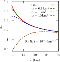
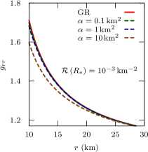
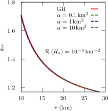
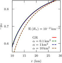
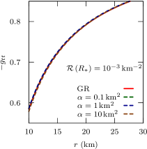
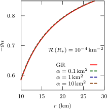
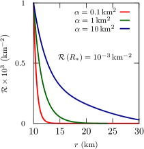
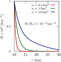
Figure 1: The metric components and the Ricci scalar for different values of $\alpha$ and $\mathcal{R}_{*}$. In all graphs, the mass of the star is assumed $1.4\,M_{\odot}$ where $M_{\odot}$ is the solar mass, and the radius of the star is assumed $R_{*}=10\,{\rm km}$.

The singular points of the metric components are $r=0$ and $r=2M=R_{\rm sch}$ as is the case in Schwarzschild’s solution. So, our solutions do not alter the location of the event horizon. The authors of Ref. Cañate et al. (2016) showed that the Ricci scalar should be zero at the Schwarzschild radius in the Starobinsky model for the spherically symmetric and static configuration. So, the outer solutions are valid from infinity to the event horizon, and the solutions given in Eqs. (39)-(41) reduce to Schwarzschild’s solution. Then, Schwarzschild’s solution describes the vacuum solution around a static black hole in Starobinsky model when the second term Eq. (1) is assumed to be a perturbative correction to GR.

V Conclusion

In this paper, we solved the vacuum field equations around a spherically symmetric and static object in the Starobinsky model by using the MAE method. We showed that the boundary layer can occur only near the surface of the star. Inside the boundary layer the solutions can be different from Schwarzschild’s solution while the metric definitely matches the Schwarzschild solution outside the boundary layer.

We thus conclude that vacuum solutions are not unique in the Starobinsky model. Our solutions have arbitrary constants which can be determined depending on the value of the Ricci scalar at the surface of the star. For some cases, the metric can be different from the Schwarzschild metric near the surface of the star. With the specific choice that the Ricci scalar is zero at the surface of the star, a boundary layer does not occur and the Schwarzschild metric is valid all over the vacuum. Another case for which a boundary layer does not occur is the choice of the boundary condition such that the first derivative of the Ricci scalar is zero at the surface of the star. Accordingly, the radius of the star and the value of the Ricci scalar at the surface as well as the mass of the star are required to uniquely define the metric outside spherically symmetric and static stars in the Starobinsky model while only mass is required in GR. The Ricci scalar is a geometric parameter rather than an observable or measurable parameter like the mass and the radius. So, it is reasonable to expect that there is a unique value of the Ricci scalar for all objects or it depends on another parameter of the object such as its compactness. Showing this is beyond the scope of this paper.

The vacuum solutions found by Ref. Cooney et al. (2010) reduce to Schwarzschild’s solution in the absence of the cosmological constant. The regular perturbation approach the authors have employed only provide solutions for the metric outside the boundary layer, and so they miss the solutions other than Schwarzschild’s solutions. This is yet another example which shows the requirement of using the MAE method when the second term in the Lagrangian is assumed to be perturbative.

Our vacuum solutions are different from the solutions obtained in Aparicio Resco et al. (2016) for the Starobinsky model as well. We considered $\alpha$ to be positive to avoid “ghosts” while their solutions are valid only when $\alpha$ is negative. Still, we could obtain such type of solutions, reincreasing the absolute value of the Ricci scalar, by proposing the boundary layer at somewhere other than the surface of the star. Yet, this case corresponds to increase of gravity with radial distance as described in Appendix A. We, thus, avoided this case purposely.

Our solution of the Ricci scalar does not contain logarithmic or some powers of $r$ as in Ref.Pun et al. (2008). The difference probably arises due to the different approaches employed or the difference between the generality of the solutions.

Within the framework of this paper, we found that the vacuum solution around a static black hole is Schwarzschild’s solution as consistent with previous studies Mayo and Bekenstein (1996); Psaltis et al. (2008); Sotiriou and Faraoni (2012); Cañate et al. (2016); Mignemi and Wiltshire (1992).

In the Starobinsky model, the interior solutions of relativistic stars also depend on the value of the Ricci scalar Arapoğlu et al. (2017) as well as the vacuum solutions. The problem being non-well posed prevents finding unique solutions. The metric components being different from that of Schwarzschild’s solution modifies the definition of the mass of the star. These issues require the simultaneous solution of the interior and the exterior metrics of the star. Therefore, the self-consistent approach which is employed in Yazadjiev et al. (2014); Staykov et al. (2014); Yazadjiev et al. (2015), can be considered as an appropriate method to study the structure of relativistic stars in the Starobinsky model. Still, the different boundary conditions cannot be distinguished far from the star, and they all satisfy the asymptotic flat space-time as shown in Fig. 1. This degeneracy reduces the reliability of using the shooting-method unless the computer code seeks for all possible solutions and does not terminate once a solution is found. Continuity of the derivative of the Ricci scalar condition at the surface of the star, given in Eq. (43), can be used to eliminate the solutions and might give a unique solution. Furthermore, it is well expected that different boundary conditions caused by vacuum solutions give different mass-radius relations for neutron stars.

Appendix A Boundary Layer at the Farthest Point

If we find the inner solutions for the boundary layer that occurred at the farthest point of a fictitious region, then follow the same steps in Sec. IV, we would obtain the vacuum solutions of the metric components as

$$f^{\rm comp}\left(r\right)= \left[1-\frac{2M}{r}\right]^{-1}+\sqrt{6\alpha C_{0}^{3}}\frac{K_{0}R_{+}}{3}\exp\left(-\sqrt{\frac{C_{0}}{6\alpha}}\left(R_{+}-r\right)\right)+\alpha\frac{5R_{+}^{2}C_{0}^{2}K_{0}^{2}}{6}\exp\left(-2\sqrt{\frac{C_{0}}{6\alpha}}\left(R_{+}-r\right)\right)$$

$$+\frac{C_{0}^{2}K_{0}}{12}\left(1-C_{0}\right)\left(R_{+}-r\right)^{2}\exp\left(-\sqrt{\frac{C_{0}}{6\alpha}}\left(R_{+}-r\right)\right)-\sqrt{\alpha}\frac{7K_{0}\sqrt{6C_{0}^{3}}}{12}\left(1-C_{0}\right)\left(R_{+}-r\right)\exp\left(-\sqrt{\frac{C_{0}}{6\alpha}}\left(R_{+}-r\right)\right)$$

$$+\alpha\left[\frac{C_{0}K_{0}}{4}\left(1-5C_{0}\right)+\frac{K_{1}C_{0}R_{+}}{3}\sqrt{6C_{0}}\right]\exp\left(-\sqrt{\frac{C_{0}}{6\alpha}}\left(R_{+}-r\right)\right),$$ (44)

$$h^{\rm comp}\left(r\right)= 1-\frac{2M}{r}+\alpha\frac{K_{0}}{C_{0}}\left(C_{0}-3\right)\exp\left(-\sqrt{\frac{C_{0}}{6\alpha}}\left(R_{+}-r\right)\right),$$ (45)

where

$$K_{0}=\frac{H_{0}}{L^{2}},\qquad K_{1}=\frac{H_{1}}{L^{3}}$$ (46)

and they are determined according to the value of the Ricci scalar at the farthest point of the region. The behaviors of the metric components are shown in Fig. 2 with two different boundary conditions where the Ricci scalar has the same magnitude but opposite sign at the farthest point of the region. It can be seen from the graphs that the metric components are independent of the sign of the Ricci scalar, and they diverge from $1$ as getting far away from the star. It means that the gravitation increases as getting far away from the star, and this is not physically reasonable.

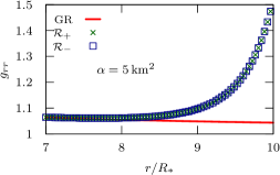
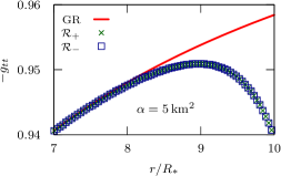
Figure 2: The metric components are shown in the case of the boundary layer occurred at the farthest point of a region. Here, the mass and the radius of the star are taken as $1.4\,M_{\odot}$ and $R_{*}=10\,{\rm km}$, respectively, where $M_{\odot}$ is the solar mass. $\mathcal{R}_{+}$ corresponds to the case where the boundary condition is chosen as positive finite value for the Ricci scalar at $r=10\,R_{*}$, and $\mathcal{R}_{-}$ corresponds to the case where the Ricci scalar at $r=10\,R_{*}$ has the same magnitude but opposite sign with the $\mathcal{R}_{+}$ case.