A Multi-band Study of the remarkable Jet in Quasar 4C+19.44

Abstract

We present arc-second-resolution data in the radio, IR, optical and X-ray for 4C+19.44 (=PKS 1354+195), the longest and straightest quasar jet with deep X-ray observations. We report results from radio images with half to one arc-second angular resolution at three frequencies, plus HST and Spitzer data. The Chandra data allow us to measure the X-ray spectral index in 10 distinct regions along the 18″ jet and compare with the radio index. The radio and X-ray spectral indices of the jet regions are consistent with a value of $\alpha=0.80$ throughout the jet, to within $2\sigma$ uncertainties. The X-ray jet structure to the south extends beyond the prominent radio jet and connects to the southern radio lobe, and there is extended X-ray emission in the direction of the unseen counter jet and coincident with the northern radio lobe. This jet is remarkable since its straight appearance over a large distance allows the geometry factors to be taken as fixed along the jet. Using the model of inverse Compton scattering of the cosmic microwave background (iC/CMB) by relativistic electrons, we find that the magnetic field strengths and Doppler factors are relatively constant along the jet. If instead the X-rays are synchrotron emission, they must arise from a population of electrons distinct from the particles producing the radio synchrotron spectrum.

1 Introduction

After more than two decades of multi-wavelength studies of extragalactic jets, there is still no clear conclusion as to the physical process responsible for the X-ray emission (Harris and Krawczynski, 2002, 2006) from powerful quasar jets which extend to 100-kpc distances. For low power jets, there is convincing evidence that X-ray emission is dominated by synchrotron radiation from electrons with Lorentz factors $\gamma$ of order 10⁷ (Worrall et al., 2001; Perlman et al., 2001; Hardcastle et al., 2001). For quasar jets, inverse Compton (iC) scattering of cosmic microwave background (CMB) photons (Tavecchio et al., 2000; Celotti et al., 2001) is generally invoked to model the X-ray emission (Siemiginowska et al., 2002; Sambruna et al., 2002, 2004; Marshall et al., 2005; Sambruna et al., 2006; Schwartz et al., 2006a, b; Worrall, 2009; Marshall et al., 2011; Perlman et al., 2011; Massaro et al., 2011). This mechanism requires that the energy distribution of the radio emitting electrons extends below $\gamma\approx$ 100 and that the jets are relativistic with bulk Lorentz factors $\Gamma\approx$ 3 to 15 (Schwartz et al., 2015). The bulk Lorentz factors are critical since the CMB energy density is enhanced in the jet rest frame by a factor $\Gamma^{2}$ (Dermer and Schlickeiser, 1994; Dermer, 1995; Ghisellini et al., 1998; Ghisellini & Celotti, 2001). For the brighter quasar jets, deep Chandra observations are capable of obtaining enough photons in spatially resolved individual regions to measure the X-ray spectral index, $\alpha_{\rm x}$, which is one of the key parameters in the iC/CMB model.

As noted above for low-power jets, iC/CMB may not be the only mechanism operating. For the quasar 3C 273, both the multi-wavelength spectra of the knots (Jester et al., 2006) and upper limits to Fermi $\gamma$-ray emission (Meyer & Georganopoulos, 2014) show that the jet must have an additional component of radiation, which might be due to synchrotron X-rays from a separate population of electrons or of protons (Aharonian, 2002). Detection of two-sided X-ray jets in the FR II radio galaxies Cyg A (Wilson et al., 2000, 2001), 3C353 (Kataoka et al., 2008), and Pictor A (Hardcastle et al., 2016) indicate a Doppler factor around unity that does not allow an iC/CMB origin. The optical polarization in the jet of the quasar PKS 1136-135 indicates production via synchrotron emission, and is best explained as arising from the low-energy tail of the X-ray emitting population (Cara et al., 2013). Meyer et al. (2015, 2017) use upper limits to Fermi $\gamma$-ray emission and also ALMA imaging of the jet in the quasar PKS 0637-752 to construct models that do not allow iC/CMB emission to explain the X-rays, providing that the ALMA and optical emission are the high energy extension of the radio synchrotron spectrum. The complex structure of the jet in the quasar PKS1127-145 requires at least two emission components, which may include both iC/CMB and synchrotron components (Siemiginowska et al., 2007).

Despite these challenges, at sufficiently large redshifts the CMB energy density must dominate over magnetic energy density, and iC/CMB X-rays will result (Schwartz, 2002). High redshift X-ray jets have been reported (Siemiginowska et al., 2003b; Cheung et al., 2006, 2012; McKeough et al., 2016), most remarkably the jet in the z=2.5 quasar B3 0727+409 for which the only radio detection is single knot 1$\farcs$4 from the core. No further extended radio emission was detected along the $\approx$ 10″ long X-ray jet (Simionescu et al., 2016). Lucchini et al. (2017) suggest that cooling of the highest energy electrons can result in X-ray jets that are ”silent in the radio and optical bands.” These considerations motivate continued efforts to test the iC/CMB model at lower redshifts.

The primary purpose of this paper is to present the broadband data collected on the 4C+19.44 jet (z=0.72). We will show that a consistent interpretation in terms of the iC/CMB mechanism is possible for the bulk of the X-ray jet. If the iC/CMB scenario is ultimately proven, it provides a means to deduce the otherwise unobservable low energy tail of the electrons producing GHz radiation. That low energy tail contains the bulk of the relativistic energy budget of the emitting particles, and must be estimated in order to apply minimum energy or equipartition arguments to measure the magnetic field.

4C+19.44 (=PKS 1354+195) was included in a Chandra and HST survey project (Sambruna et al., 2002, 2004; Marshall et al., 2005) that was based on a selection of radio jets that were asessed as having high probability of detection by Chandra in a 5 to 10 ks observation. We selected this source for longer observations because the 10 ks Chandra observation demonstrated that the entire jet to the South of the quasar was detected in the X-rays and because two inner knots were also optically-detected with the Hubble Space Telescope (HST) (Sambruna et al., 2002). Preliminary results from these longer Chandra observations have been reported (Schwartz et al., 2007a, b). In addition to the deep Chandra observations, we obtained HST observations (475 and 814 nm), a Spitzer image (3.6 $\mu$m) and data at three radio frequencies (1.4, 5, and 15 GHz) with the NRAO Very Large Array (VLA). With many resolution elements down the jet, our primary goal was to evaluate the spectral energy distributions as a function of distance from the quasar in order to constrain the emission processes for the various bands.

We adopt $h={\rm H}_{0}$/(100 km s^-1 Mpc^-1)=0.67, $\Omega_{\rm M}=0.27$ and $\Omega_{\rm\Lambda}=0.73$, so that at a redshift of 0.719 (Steidel & Sargent, 1991) 1^′′ corresponds to 7.7 kpc. Spectral indices, $\alpha$, are defined by flux density S${}_{\nu}\propto\nu^{-\alpha}$.

2 The Data

2.1 Chandra X-ray Data

Our deep Chandra observation was scheduled as four separate pointings in 2006
http://cda.harvard.edu/chaser?obsid=6903,6904,7302,7303 (catalog Chandra ObsIDs 6903, 6904, 7302, and 7303) for a total of 199 ks on target as summarized in Table 1. We observed using only the back illuminated ACIS chip S3 in a 1/4 sub-array mode to reduce the effects of pile-up of the bright nucleus. This results in a dead-time fraction of about 5% (0.04104 s readout time divided by the 0.84104 frame time) for a net observation live-time of 189.35 ks. All data were obtained with ACIS-S in the faint mode; i.e., telemetering the 3$\times$3 pixel amplitudes. A range in roll angle was requested to position the CCD charge-transfer readout streak away from the jet. ObsID 6904 gave about 35 ks live-time taken at roll angle 120°, while the remaining observations were all at 137°. Although we encountered a star tracker problem during the first half of ObsID 7302 that produced a displacement to the east, the offset was of order 0$\farcs$2 so for the purposes of photometry, we did not reject these data. Previous results were reported using CALDB 3.2.1; more recently we have reanalyzed all the data using CALDB 4.5.1.1 and CIAO 4.6. These give an appropriate ACIS contamination model, and use the energy dependent sub-pixel event redistribution algorithm (EDSER). Various members of our team have analyzed the data independently. We also add the reprocessed data from http://cda.harvard.edu/chaser?obsid=2140 (catalog Chandra ObsID 2140) originally published by Sambruna et al. (2002, 2004), to give a total live-time of 198.4 ks.

Table 1: Summary of the Chandra X-ray Observations

Observation Date	ObsID	Live Time	Roll Angle
		(ks)
2001 Jan 08	2140	9.056	66°
2006 Mar 20	6904	34.958	120°
2006 Mar 28	7302	68.936	137°
2006 Mar 30	7303	41.523	137°
2006 Apr 01	6903	43.933	137°

An alternate analysis was reported in Massaro et al. (2011). They created flux maps in the soft (0.5–1 keV), medium (1–2 keV), and hard (2–7 keV) bands. For each band, the data were divided by the exposure map and multiplied by the nominal energy of each band, resulting in maps with units of erg cm^-2 s^-1. Photometry was then performed for each region using funtools and is reported in the on-line version of Table 7 of Massaro et al. (2011) for ObsID 7302.

Table 2: Photometric Regions

Description	shape	Position	Size
		(J2000.0)
N16.0; N hot spot	box	13:57:04.174,+19:19:22.54	2$\farcs$46,1$\farcs$72,163∘
N15.4; N lobe	circle	13:57:03.959,+19:19:21.06	6$\farcs$4
S2.1	box	13:57:04.476,+19:19:05.36	2$\farcs$12,1$\farcs$72,163∘
S4.0	box	13:57:04.507,+19:19:03.57	1$\farcs$54,1$\farcs$72,163∘
S5.3	box	13:57:04.531,+19:19:02.30	1$\farcs$08,1$\farcs$72,163∘
S6.6	box	13:57:04.540,+19:19:00.97	1$\farcs$52,1$\farcs$47,163∘
S8.3	box	13:57:04.583,+19:18:59.37	1$\farcs$87,1$\farcs$72,163∘
S10.0	box	13:57:04.613,+19:18:57.81	1$\farcs$38,1$\farcs$72,163∘
S11.2	box	13:57:04.661,+19:18:56.65	1$\farcs$23,1$\farcs$72,163∘
S12.9	box	13:57:04.697,+19:18:55.20	1$\farcs$87,1$\farcs$72,163∘
S14.6	box	13:57:04.732,+19:18:53.58	1$\farcs$47,1$\farcs$72,163∘
S15.9	box	13:57:04.760,+19:18:52.29	1$\farcs$23,1$\farcs$72,163∘
S17.7	box	13:57:04.800,+19:18:50.50	2$\farcs$46,1$\farcs$72,163∘
S21.6; transition region	box	13:57:04.799,+19:18:46.37	5$\farcs$4,5$\farcs$4,163∘
S25.7; entrance SHS	circle	13:57:04.887,+19:18:42.52	1$\farcs$33
S28.0; S hot spot	circle	13:57:04.780,+19:18:39.89	1$\farcs$72
North Background	box	13:57:03.568,+19:19:55.93	35$\farcs$04,49$\farcs$35,0∘
Southwest Background	box	13:57:03.422,+19:18:24.28,	24$\farcs$26,24$\farcs$05,315∘

2.1.1 Photometric Regions

Since our primary interest is to determine the spectral energy distribution (SED) for each X-ray feature, we defined our regions on the basis of the X-ray morphology. The regions are shown in figure 1 and are labeled with their direction (N or S) and distance in arc-seconds of the region center from the quasar, following the convention defined in Schwartz et al. (2000). Each ObsID was adjusted by an amount between 0$\farcs$21 and 0$\farcs$30 to superpose the quasar core at the position given in Johnston et al. (1995); RA:13^h57^m04.4366^s and DEC:+19^∘19′07$\farcs$372  (J2000). N16.0 is a rectangle for the northern hot-spot and N15.4 is a large circle to deal with the northern lobe. Moving south from the quasar, the first region is designated S2.1 and there are a total of 11 rectangles along the jet. S6.6 is not centered on the jet: the eastern 0$\farcs$25 has been trimmed off in order to avoid optical emission associated with a (foreground?) edge-on galaxy. After the main jet, there is a large square, S21.6 which is termed ‘the transition region’. It contains low brightness emission in both X-ray and radio bands: although the morphology is not well defined, the emission may arise from the southern lobe. Finally there are two circular regions, S25.7, called ‘the entrance to the hot-spot’ and S28.0, the southern hot-spot itself. The regions are shown in Figure 1 and specified in Table 2. Detector background was determined from two large rectangular regions, north of the northern lobe and southwest of the southern lobe. These are not shown, but are specified in Table 2. Table 3 gives the resulting 1 keV flux densities for all the regions, along with those at other frequencies as discussed in sections 2.2, 2.3, and 2.4.

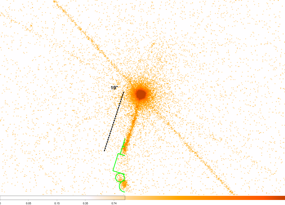
Figure 1: The regions defined by the X-ray morphology, and used for photometry are delineated by the solid circles and rectangles defined in Table 2. The figure is a summed X-ray count map (0.5–7 keV) binned in 0$\farcs$246 $\times$ 0$\farcs$246 pixels. From top (North) to bottom, N16.0 is the small rectangle for the northern hot-spot, and N15.4 is the large circle for the northern lobe. The bright and the faint streaks from NE to SW are the CCD readout streaks from the observations at the two different roll angles. The jet is composed of the 11 rectangular regions starting 2$\farcs$1 S of the quasar nucleus and ending at S17.7. The large rectangle, S21.6 is the ‘transition region’ which has only low surface brightness in both the radio and X-ray bands. The next region is a small circle, S25.7 which is the ‘entrance’ to the S hot-spot, and the last, larger circle is the S hot-spot. Numbers in the name of each region refer to the center of the box or circle. The color bar gives counts per pixel, and saturates at 50 counts per 0.0605 arc-second².

2.1.2 Spectral Analysis

Modeling of the X-ray emission from several regions has been performed in Sherpa (Freeman et al., 2001) version CIAO 4.6. We extracted the spectra and created response files for each observation and used the energy range 0.5–7 keV for all the spectral modeling. The number of net counts from the jet in each region, used for the photometry reported in Table tab:fluxes, ranged from 39.3 to 184.5, after subtracting the detector background and scattered photons from the quasar itself. We determined the latter from a Marx 5.1 simulation of the quasar, using the quasar’s measured spectral energy index, $\alpha_{\rm x}$, of 0.66 (Marshall et al., 2017), and incorporating pile-up, the ACIS readout streak, and EDSER. In region S2.1 the quasar can account for the entire signal, leaving the ten regions from S4.0 to S17.7 for analysis of the jet. For spectral fitting we neglected the background counts, predicted to range from 1.2 to 2.6, i.e., less than 2% of the total counts in any region. Scattered photons from the quasar give 44% and 39% of the counts in regions S4.0 and S5.3, but should bias the fit to the index by less than the estimated errors, since the quasar has a similar spectrum. We used the Nelder-Mead optimization algorithm and Cash likelihood statistics appropriate for low counts and fit the data in Sherpa.

For the spectral analysis we use only the four contemporaneous ObsID’s from 2006 (Table 1). We fit the same model jointly to the four individual spectra. We assumed an absorbed power law model for each region, with the absorption column frozen at the Galactic value of $\rm N_{H}=2.23\times 10^{20}$ cm^-2. No absorption in excess of Galactic was detected, with 90% upper limits for an absorber at redshift ${\it z}=0.5$ with a range of $(0.2$ to $0.4)\times 10^{22}$ cm^-2 for the different regions. We then froze the excess absorption at zero, and fit the photon index $\Gamma$ of a power law and the normalization. We get the same results using XSPEC or Sherpa. Table 4 lists the X-ray spectral results, reporting the energy index $\alpha_{\rm x}=\Gamma-1$, along with the radio spectral index as discussed in section 2.4.1.

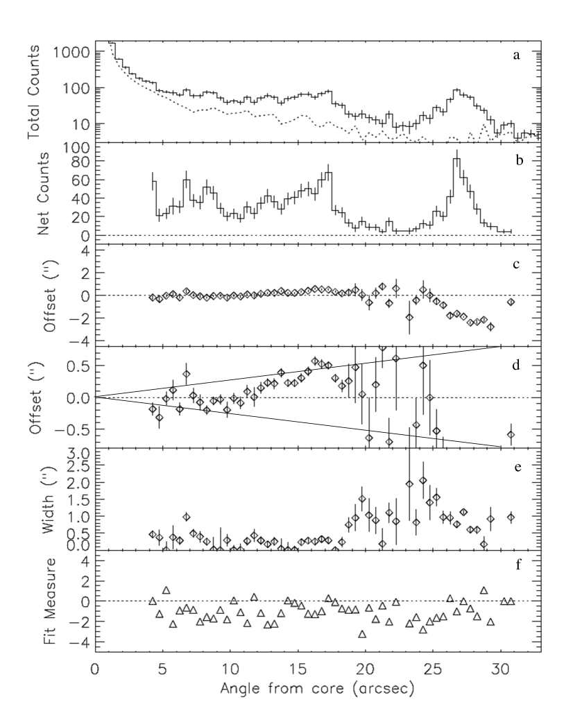
Figure 2: Panel a: solid histogram gives Chandra X-ray counts per bin along the jet through the southern hotspots. Dashed histogram gives counts per bin in a region 180° from the jet. Panel b: net counts, subtracting the region 180° away. Panel c: the deviation of the centroid of each bin from the mean position angle of 165°. Panel d is the same data plotted at a stretched scale to emphasize the inner straight 17″ jet, and with the solid lines indicating a deviation of $\pm$1$.\!^{\circ}$5 from 165°. Panel e: The width, defined as the difference in quadrature of a fit to the observed data plus background, and the intrinsic resolution $\sigma=0\farcs 34$ determined from the readout streak. Panel f: the fit measure is calculated from the probability determined from a Kolmogorov-Smirnov goodness of fit test, converted to a Gaussian deviate giving the same probability.

2.1.3 X-ray Jet Structure

We generated profiles of the X-ray jet, using likelihood-based Gaussian fitting with Poisson statistics. We sorted the summed counts from 0.5 to 7 keV into 0$\farcs$5 bins along the jet, taking counts $\pm$5″ perpendicular to the jet. Figure 2 plots the data along the jet as a function of distance from the quasar core. Each fit was to a one dimensional Gaussian normal to the jet, with free parameters being the total number of counts, the position relative to the mean position angle of 165°, the sigma of the Gaussian, and the background level data from a strip at position angle 345°. Small aspect residuals were reduced by fitting the quasar core in right ascension and declination in separate 300 s time intervals, and fitting the residuals from the known position to a polynomial to correct the data. Fitting a Gaussian shape across the ACIS readout streak gives $\sigma$= 0$\farcs$34, and represents the intrinsic response to an unresolved line source. Subtracting this number in quadrature from the standard deviation gives a measure of the intrinsic width of the jet, plotted in the second panel up from the bottom.

Closer than 3$\farcs$5 from the quasar the jet parameters cannot be determined. The width is marginally resolved in the 3$\farcs$5 to 17″ region, but contaminated due to the galaxy SDSS J135704.63+191900.9 which has a significant X-ray flux density $\approx$0.08 nJy, and overlaps the jet in the 6″ to 7″ region. The X-ray emission is clearly detected and very broad between 20″ and 25″. This region bridges the straight part of the jet and the terminal hot-spot, and is probably part of a lobe structure. Within the 17″ jet there are some significant, but small, offsets of the position angle of the jet center line (middle panels of Figure 2).

2.2 HST Data

Our HST data were obtained with the WFC-ACS (proposal ID 10762) on 2006 March 23 (F814W) and March 24 (F475W). Exposure times were 6998 s and 4472 s respectively. We also included analysis of some archival WFPC2 F702W data from 1996 Jun 22 (4600 s exposure; proposal ID 5984). The images were processed in the usual manner with CAL_VER 4.6.1. The 8060Å image is shown in Figure 3.

The left panel shows the field around the quasar. The presence of many galaxies of similar size and magnitude (particularly to the East of the quasar) is suggestive of a group or cluster. Ellingson et al. (1991) searched for a cluster associated with 4C+19.44 and studied seven galaxies within 2′ of which four had measured redshifts between 0.36 and 0.53. The NASA/IPAC Extragalactic Database (NED) indicates that 4C+19.44 has absorption line systems at z = 0.431, 0.457, and 0.522 (Ryabinkov, Kaminker, & Varshalovich, 2003). There are three galaxies listed by NED that lie within 30^′′; these have spectroscopic redshifts in the range z = 0.43- 0.46, while the SDSS-measured redshift of 4C+19.44 is 0.7196 (Schneider et al., 2010). There are no other objects within 4′ that have SDSS spectra. Attempts to confirm either a foreground cluster or a cluster associated with the quasar using SDSS photometric redshifts were inconclusive. The measured X-ray profile in an azimuthal sector of 70° to the West tracks the profile of the simulated point quasar plus background, and puts a 2$\sigma$ upper limit of 2$\times$10⁴³ erg cm^-2 s^-1 for emission from an assumed cluster with temperature 2 keV at the redshift of the quasar.

The other two panels of Figure 3 have had their contrasts adjusted to emphasize the optical detections of knots within regions S2.1 and S4.0. We find that S2.1 has an apparent diameter of 0$\farcs$2, consistent with the deconvolved radio major axis, whereas S4.0 has an extent along the jet of $\approx$ 0$\farcs$4, again consistent with the radio size in the PA of the jet. Emission from the region S5.3 is also significant although barely visible in Figure 3. The HST photometry reported in Table 3 was performed on images that had a first order subtraction of the quasar.

Figure 3: Left panel: The HST F475W image with 1.4 GHz radio contours overlaid. Middle panel: HST F814W image with 5 GHz contours from the the VLA A array overlaid. The grey scale mapping is adjusted to show the knot S2.1. Right panel: Same data as the middle panel, but with the field of view and grey scale adjusted to show the detection of S4.0. S5.3 is also detected in all three HST filters. The lowest radio contour is 0.25 mJy/beam with contours increasing by factors of 4.

Table 3: Flux densities for X-ray defined regions

Region	4.86 GHz	14.9 GHz	3.6 $\mu$m	F814W	F702W	F475W	1.0 keV
	4.9 109 Hz	1.5 1010 Hz	8.3 1013 Hz	3.7 1014 Hz	4.3 1014 Hz	6.3 1014 Hz	2.4 1017 Hz
	(mJy)	(mJy)	($\mu$Jy)	($\mu$Jy)	($\mu$Jy)	($\mu$Jy)	(nJy)
N16.0	61.1$\pm$0.30	23.7$\pm$0.4	$\cdots$	$<$0.52	$<$0.24	$<$0.12	0.101$\pm$.028
N15.4	173$\pm$20	48.2$\pm$2.5	$\cdots$	$<$15	$<$6.2	$<$3.8	0.822$\pm$0.111
S2.1	$\cdots$	$\cdots$	$\cdots$	0.57$\pm$0.09	0.40$\pm$0.15	0.21$\pm$0.07	$<$0.42
S4.0	16.5$\pm$0.20	7.21$\pm$0.36	$\cdots$	0.11$\pm$0.01	0.07$\pm$0.04	0.07$\pm$0.02	0.513$\pm$0.079
S5.3	6.69$\pm$0.21	2.92$\pm$0.28	$\cdots$	0.07$\pm$0.03	0.08$\pm$0.03	0.04$\pm$0.01	0.184$\pm$0.045
S6.6	11.0$\pm$0.20	4.57$\pm$0.33	$<$10	$<$0.28	$<$0.26	$<$0.11	0.396$\pm$0.051
S8.3	19.0$\pm$0.30	7.56$\pm$0.39	$<$10	$<$2.59	$<$1.64	$<$0.33	0.693$\pm$0.062
S10.0	6.19$\pm$0.23	2.29$\pm$0.34	$<$10	$<$1.74	$<$0.59	$<$0.84	0.302$\pm$0.042
S11.2	5.34$\pm$0.22	2.00$\pm$0.32	$<$6	$<$0.14	$<$0.07	$<$0.10	0.310$\pm$0.041
S12.9	9.91$\pm$0.27	4.11$\pm$0.39	$<$12	$<$1.94	$<$1.05	$<$0.55	0.643$\pm$0.058
S14.6	9.18$\pm$0.24	3.48$\pm$0.35	$<$6	$<$0.10	$<$0.23	$<$0.10	0.604$\pm$0.054
S15.9	2.79$\pm$0.22	1.10$\pm$0.32	$<$6	$<$0.10	$<$0.12	$<$0.08	0.581$\pm$0.053
S17.7	2.48$\pm$0.31	0.87$\pm$0.45	$<$6	$<$0.12	$<$0.10	$<$0.06	0.865$\pm$0.065
S21.6	5.45$\pm$0.82	3.01$\pm$1.18	$\cdots$	$<$1.1	$<$0.83	$<$0.52	0.434$\pm$0.056
S25.7	3.17$\pm$0.35	1.50$\pm$0.51	$<$6	$<$0.33	$<$0.46	$<$0.08	0.392$\pm$0.045
S28.0	85.7$\pm$0.5	30.4$\pm$0.7	$<$6	$<$0.60	$<$0.52	$<$0.38	1.09$\pm$0.074

Note. — X-ray flux densities were derived from the observed fluxes assuming an energy index $\alpha_{\rm x}$=0.8.

2.3 Spitzer IRAC Data

Our Spitzer IRAC data were taken on 2005 July 16 as part of our Cycle-1 General Observer program (Uchiyama et al., 2006). We chose the pair of 3.6 and $5.8\ \mu\rm m$ arrays for best spatial resolution and sensitivity. The native pixel size in both arrays is $\simeq 1\farcs 22$, and the point spread functions are $1\farcs 66$ and $1\farcs 88$ (FWHM) for the 3.6 and $5.8\ \mu\rm m$ bands, respectively. We obtained a total of 60 frames per channel, each with a 30-s frame time, and the frame data were combined into a single image using the Spitzer Science Center software mopex. We subtracted the PSF wing of the bright quasar core from each IRAC image. Also, some field galaxies (see the Hubble image) near the southern jet were subtracted.

Figure 4: Spitzer IRAC 3.6 micron image, with the X-ray photometry regions overlaid. All apparent emission can be attributed to the quasar and foreground galaxies. The jet surface brightness is too low to detect with the angular resolution of Spitzer.

No significant infrared emission was found along the jet with the Spitzer IRAC (Figure 4). Based on statistical fluctuations of the surface brightness of the core-subtracted IRAC image and the uncertainties associated with PSF removal (adopting 10% of the quasar’s PSF wing intensity at the location being considered), we place a $3\sigma$ upper limit on the $3.6\ \mu\rm m$ flux of a point source in this region as $f_{3.6}=6\ \mu\rm Jy$. As reported in Table 3, we adopt this value as the upper limit for each jet knot and hot-spot except that we place more conservative limits for some regions that contain field galaxies (S6.6, S8.3, S10.0, and S12.9). We do not report the upper limits for the $5.8\ \mu\rm m$ band because they are much less constraining.

2.4 VLA Observations

We have performed radio observations of the quasar with the NRAO VLA (program S71062) at two epochs: 2006 February 06 at 1.4 and 4.86 GHz with A-array and 2006 July 30 at 4.86 and 14.965 GHz with B-array. The data were reduced in the usual manner with the Astronomical Image Processing System (AIPS) using 1407+284 as a phase and polarization D-terms calibrator and 3C 286 as an amplitude and polarization position angle calibrator. We also use Difmap for modeling calibrated uv-data. We have obtained images for three Stokes parameters, I, Q, and U. At 1.4 GHz we have imaged separately the two intermediate frequency bands centered on 1.365 GHz and 1.435 GHz. Table 5 summarizes the radio observations. The highest dynamic-range image of the quasar is presented in Figure 5, which shows that the morphology of the radio source is similar to the X-ray structure: a bright compact core, a prominent jet to the south-east up to 17^′′ from the core at position angle $\sim$165^∘, a southern hot spot with faint diffuse emission, and a diffuse northern lobe with a hot spot. We have measured the flux at all wavelengths in the photometric regions described in section 2.1.1 using the AIPS task IMEAN. The measurements at 4.86 GHz and 14.9 GHz are listed in Table 3, for the regions defined in Table 2. At 1.4 GHz the beam size is large enough that some of the flux density “spills” out of the smaller photometric regions.

Figure 5: VLA image at 4.86 GHz (B-array). The parameters of the image are given in Table 5; contours increase by factors of 2 and the lowest contour level is 0.2 mJy/beam.

Figure 6: VLA images at different wavelengths: left - at 1.365 GHz (A-Array, lowest contour is 0.45 mJy/beam), middle - at 4.86 GHz (A-Array, lowest contour is 0.2 mJy/beam), and right - at 14.965  GHz (B-Array, lowest contour is 0.3 mJy/beam). The parameters of the image are given in Table 5; contours increase by factors of 2; linear segments show polarization E-vectors; the length of vectors is proportional to the local polarized intensity.

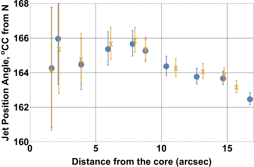
Figure 7: Dependence of position angle (top) and width (bottom) of the jet on distance from the core at 5 GHz (filled circles) and 15 GHz (crosses). These quantities are measured from 2-d components using modelfit in difmap. The jet appears wider than in X-rays, but note the different modeling technique (1-d cross-cuts) in the X-ray case.

Figure 8: Radio profiles (from top to bottom) of: 1. The total intensity (solid curve) and percent polarization (values are divided by a factor of 4, dotted curve) at 5 GHz; 2. The spectral index between 1.4 and 15 GHz; 3. The position angle of polarization (electric vector) at 5 GHz (solid curve) and 1.4 GHz (dotted curve); 4. The Faraday rotation measure.

Table 4: Radio and X-ray Spectral Results for the X-Ray Jet Regions

Region	$\alpha_{R}$	$\alpha_{Rerr}$	$\alpha_{\rm X}$	$\alpha_{\rm Xerr}$
		1 sigma		1 sigma
S4.0	0.74	$\pm$0.05	0.55	$\pm$0.13
S5.3	0.74	$\pm$0.09	0.90	$\pm$0.22
S6.6	0.78	$\pm$0.07	0.87	$\pm$0.18
S8.3	0.82	$\pm$0.05	0.64	$\pm$0.14
S10.0	0.88	$\pm$0.14	0.61	$\pm$0.20
S11.2	0.87	$\pm$0.15	0.68	$\pm$0.21
S12.9	0.78	$\pm$0.09	0.93	$\pm$0.16
S14.6	0.86	$\pm$0.09	0.88	$\pm$0.17
S15.9	0.83	$\pm$0.27	0.81	$\pm$0.16
S17.7	0.93	$\pm$0.47	0.81	$\pm$0.13

Table 5: Summary of the VLA Observations

Frequency	Array	TOS	Clean Beam	I Map Peak	I rms	P Map Peak	P rms
(GHz)				(mJy/Beam)	(mJy)	(mJy/Beam)	(mJy)
1.365	A	4h10m	1.21$\times$1.07, 50.6	1240	0.012	71.9	0.063
1.435	A	4h10m	1.16$\times$1.03, 48.4	1210	0.028	71.1	0.075
4.860	A	4h10m	0.47$\times$0.43, 38.5	1164	0.073	49.6	0.039
4.860	B	3h31m	1.09$\times$1.06, 19.2	1171	0.061	51.5	0.078
14.940	B	5h21m	0.50$\times$0.49, 36.4	1805	0.096	34.0	0.088

2.4.1 Radio Jet

Figure 6 shows total intensity images of the jet with linear polarization electric vectors. The jet has knotty structure, which we have modeled as circular Gaussian brightness distributions using the task MODELFIT in Difmap. For each component we have obtained angular distance, $R$, and position angle, $\Theta$, relative to the core located at RA: 13^h57^m04.4366^s and DEC:+19^∘19′07$\farcs$372  (J2000), as well as FWHM size, $w$, and flux density, $S$. The number of components required to fit the data was determined by the best agreement between the model and data according to $\chi^{2}$ values. In general, 10 Gaussian components give a reasonable representation of the jet morphology at all frequencies, with reduced $\chi^{2}$ ranging from 1.5 to 5. Figure 7 shows the dependence of $\Theta$ and $w$ on distance from the core. We estimate 0$\farcs$1 uncertainty in position or width, so that the position angle error is 0$\farcs$1/(distance in radians). Although the jet executes wiggles close to the core, deviations do not exceed the uncertainties, and, on average, the jet is straight within 9^′′ of the core, with $\Theta$=165.0${}^{\circ}\pm$0.5^∘. Beyond 9^′′ it turns to the east by 1.5${}^{\circ}\pm$0.5^∘ relative to the core, or $\sim$4^∘ with respect to the previous direction. The independence of the width of the jet on distance indicates that the jet is well collimated, with similar size near the core and at the end (at 17^′′ or 130 kpc in projection from the core). However, in the transverse direction the jet appears to undergo contractions and expansions. These could be the result of standing shock formation in the jet flow as it adjusts to imbalances between the jet and external medium pressures, as seen in numerical simulations (Aloy et al., 2003). Both properties (good collimation and contraction-rarefaction structure) imply that the jet should be highly supersonic and probably relativistic far downstream of the core.

We have constructed profiles along the jet axis of total intensity, degree of polarization, spectral index, position angle of polarization, and Faraday rotation measure ($RM$), as plotted in Figure 8. Each point of a profile is the median average within a window of half a beam size. The window slides by half of its size for every new measurement. There is a prominent feature in the polarization profiles in the region from 7^′′ to 10^′′. The profiles at all wavelengths show an increase of total intensity, a sharp decrease of degree of polarization, and a change of position angle of polarization in this region. In addition, the change of position angle of polarization depends on wavelength. Such behavior can result from an increase of $RM$, in this part of the jet. We have calculated the $RM$ values using polarization maps at 1.365, 1.435, 4.86, and 14.965 GHz, convolved with the same circular beam of 1^′′$\times$1^′′ for the polarized intensity exceeding the 3$\sigma$ rms level. At 14.965 GHz this condition applies only within $\sim$5^′′ from the core. The average rotation measure is low, $\sim~{}5$ rad m^-2, being consistent with integrated measurements and likely of Galactic origin (Simard-Normandin et al., 1981). However, the RM increases by a factor of 2 in the core and by a factor of 5 in the region from 7^′′ to 10^′′ and at the end of the jet. The HST image (see Figure 3) contains a galaxy partially projected on the jet 6^′′-7^′′ from the core. The gas from the galaxy could cause the observed polarization behavior if the galaxy lies along the line of sight to the quasar. On the other hand, the brightening is difficult to explain if the galaxy is intervening rather than interacting with the jet. In the former case, the increase in the intensity must be intrinsic. Because of this ambiguity, we exclude the region affected by the galaxy and also the core region within 1$\farcs$5 (the core has degree of polarization $P^{\rm core}_{\rm 5~{}GHz}\sim$4%) from all further discussion of the jet radio properties.

The total intensity along the jet varies by a factor of $\sim$50 while the degree of polarization changes by a factor of $\sim$3. There is a tight correlation between the total and polarized intensity in the jet, with linear coefficient of correlation $\rho=0.94$; however, the degree of polarization does not correlate with total intensity ($\rho=0.13$). On average, the jet is highly polarized, with $\langle P_{5GHz}\rangle$=(24.7$\pm$6.0)% and polarization position angle $\langle\chi_{5GHz}\rangle$=(84$\pm$6)^∘. These values indicate that the magnetic field aligns with the jet direction and that the degree of field order remains fairly uniform along the jet. Nevertheless, comparison of the variations in polarization position angle (Figure 9), defined as $\Delta\chi=\left\|\chi-\langle\chi\rangle\right\|$, with the total intensity behavior along the jet suggests a positive correlation between the two ($\rho=0.37$). This correlation can be explained if the magnetic field tends to be more turbulent in bright knots than in the underlying jet. We caution, however, that the maximum variations of $\chi$ are only $\sim$10^∘, while the uncertainties of individual measurements of polarization position angle are $\sim$5^∘.

Figure 9: Top: Profiles of variations of polarization position angle (solid curve) and total intensity (dotted curve) at 5 GHz. Bottom: Normalized profiles of spectral index (solid curve), $\langle\alpha_{\rm r}\rangle$=0.73, and total intensity (dotted curve), $\langle S\rangle$=3.4 mJy/Beam.

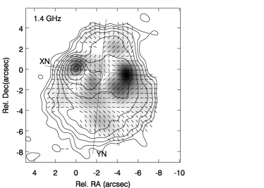
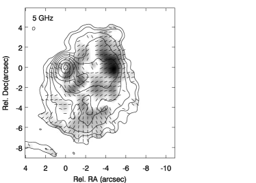
q

Figure 10: top: Total (contours) and polarized (gray scale) intensity images of the northern lobe. left: at 1.4 GHz (A-array), $S_{\rm peak}$=101.3 mJy/beam, $S_{\rm peak}^{\rm pol}$=4.16 mJy/beam, and right: at 5 GHz (B-array), $S_{\rm peak}$=33.4 mJy/beam, $S_{\rm peak}^{\rm pol}$=1.81 mJy/beam. Beam size is according to Table 5; linear segments correspond to polarization E-vectors; solid lines in left panel show two axes XN and YN used for constructions of profiles in the lower left and right panels, respectively. bottom: Those profiles show (top to bottom) 1. Total intensity at 1.4 GHz; 2. Spectral index between 1.4 and 5 GHz; 3. Degree of polarization at 1.4 GHz; 4. Position angle of polarization at 1.4 GHz.

We have calculated the radio spectral index, $\alpha_{\rm R}$, using flux densities at 1.365, 1.435, 4.86, and 14.965 GHz from images convolved with the same beam of 1^′′$\times$1^′′ . We find an inverted spectrum in the core $\alpha_{\rm R}^{core}=-0.14\pm 0.07$, an optically thin spectrum in the jet, $\langle\alpha_{\rm R}\rangle=0.82\pm 0.06$, and a steeper spectrum near the end of the jet (beyond 15.5^′′),  $\alpha_{\rm R}>$1.0. There are small variations of $\alpha_{\rm R}$ along the jet between 1$\farcs$5 and 15$\farcs$5 from 0.74 to 0.93 with the uncertainty of individual measurements from $\pm$0.05 up to $\pm$0.5. These variations show a possible anti-correlation with total intensity ($\rho=-0.30$, see also Figure 9), which implies a slightly harder radio spectrum within bright knots. Table 4 gives the separate radio and X-ray spectral indices and their 1$\sigma$ errors in the ten regions used for X-ray photometry of the jet. All are consistent with the value 0.80, considering the uncertainties. The X-ray spectral index of the quasar core is slightly flatter, $\alpha_{\rm x}=0.66^{+0.07}_{-0.06}$ (Marshall et al. 2017, ApJS, submitted).

2.4.2 Radio Lobes

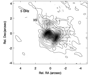
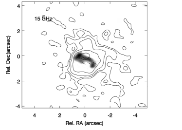
Figure 11: Top: Total (contours) and polarized (gray scale) intensity images of the southern lobe left: at 5 GHz (A-array), $S_{\rm peak}$=6.76 mJy/beam, $S_{\rm peak}^{\rm pol}$=1.40 mJy/beam, and right: at 15 GHz (B-array), $S_{\rm peak}$=2.94 mJy/beam, $S_{\rm peak}^{\rm pol}$=0.89 mJy/beam. Beam size is according to Table 5; linear segments correspond to polarization E-vectors. Bottom: Radio profiles of the southern lobe along axis XS in the top left panel. From top to bottom; Total intensity at 5 GHz; Spectral index between 5 and 15 GHz; Degree of polarization at 5 GHz; Position angle of polarization at 5 GHz.

The northern radio lobe (Figure 5) is located $\sim$16^′′ from the quasar at the position angle
$\Theta$ $\sim$ - 14^∘, which corresponds to the direction of the inferred counter-jet. Figure 10 shows the total and polarized intensity structure of the lobe. There are two prominent features: a bright knot in total intensity (hot spot) and a separate bright knot in polarized intensity (polarized spot) located  4^′′ to the west from the hot spot. We have constructed the total intensity and degree of polarization profiles at 1.4 GHz along the line connecting the knots (axis XN) and along the line perpendicular to the juncture (axis YN) (see Figure 10), as well as spectral index profiles using 1.4 GHz and 5 GHz maps obtained with similar resolution beams. The spectral index profiles show that $\alpha_{1.4-5GHz}$=1.1$\pm$0.1 dominates the diffuse part of the lobe except two regions: i) the region at the western end beyond the polarized spot with the steepest spectrum ($\alpha\sim$1.4) and ii) the region on the northern end with the flattest spectrum ($\alpha\sim 0.7$). The hot spot also has a fairly hard spectrum, $\alpha\sim 0.8$. The degree of polarization in the hot spot is low, $P\sim 2\%$, perhaps due to rotation of the magnetic field direction within the beam as seen from the $\chi$ profile. The northern edge has an increase of degree of polarization up to 30% and position angle of polarization perpendicular to the boundary, i.e., the magnetic field ordered along the boundary (assuming a small $RM$). These conditions, along with hardening of the spectrum imply a shock formation on the northern end. It is difficult to understand the nature of the polarized spot that has similar surface brightness to the neighboring region, a steep spectrum ($\alpha\sim 1.1$), high polarization $\sim$20-30%, and fairly uniform magnetic field along the YN axis. In general, the magnetic field in the lobe has patchy structure, with the size of a patch $\sim$2^′′$\times$2^′′ and uniform magnetic field within a patch, with changing direction from one patch to another.

The diffuse part of the southern lobe is most likely located between the end of the jet and the southern hot spot, with too low a radio surface brightness to be seen in our high resolution maps, (e.g. Figure 5). The hot spot is located 28^′′ from the core at $\Theta\sim$170^∘, shifted by $\sim$5^∘ from the jet direction. The high resolution maps (Figure 11) show that the hot spot has a double structure with a separation between peaks $\sim$0.7^′′. We have constructed profiles along the line crossing the peaks, (axis XS in Figure 11), similar those obtained for the northern lobe; the profiles are presented in the bottom section of Figure 11. The spectral index ($\alpha_{5-15GHz}$) of the region is similar to that of the jet. The magnetic field is rather uniform with the direction perpendicular to XS axis, the polarized intensity increases in the peaks, and the whole structure has an almost constant degree of polarization $\sim$20%.

2.4.3 VLBA 2cm Survey Data

Three epochs (1997.63, 1999.55 and 2002.61) of 15 GHz VLBA observations were obtained as part of the VLBA 2 cm survey (Kellermann et al., 2004; Zensus et al., 2002). Since no published VLBI proper motions were available in the literature, we obtained the calibrated ($u,v$) data from the MOJAVE website (Lister et al., 2009) and modeled them with circular Gaussians using Difmap to fit knot positions. Two distinct knots are found with average separations of $\sim$3 mas and $\sim$5.5 mas from the core during these epochs. These components are well fitted with proper motions of 0.20 mas/yr and 0.23 mas/yr, at average position angles of 145°and 142°, respectively (c.f. PA=165° for the kpc scale jet); see Figure 12. These translate to apparent motions of $(8.1\pm 1.2)c$ and $(9.4\pm 1.2)c$, where the uncertainties assumed 0.1 mas errors in determinations of the knot positions. Marshall et al. (2017) use an additional VLBA measurement in 2003.01 to estimate velocities 8.68$\pm$0.4 c and 9.84$\pm$0.7 c, respectively, for the inner and outer knots.

The apparent superluminal proper motions require the pc-scale jet to be aligned at $<14\arcdeg$ (3 mas knot) and $<12\arcdeg$ (5.5 mas knot) to our line-of-sight. The observed difference in the projected position angles of the outermost VLBI-scale knot and the kpc-scale jet of $23\arcdeg$ is likely caused by a smaller intrinsic bend in the jet amplified by projection. For small observed misalignments, the intrinsic bend in the jet is probably smaller than the angle to the line-of-sight (see Conway & Murphy, 1993; Marshall et al., 2011; Singal, 2016). In this case, we take an intrinsic bend of $\sim 23\arcdeg$ sin ($12\arcdeg$) $\sim 5\arcdeg$ in the jet to estimate that the kpc-scale jet is likely aligned at $\leq 12\arcdeg$ to our line-of-sight, consistent with estimates to be presented in Section 4.

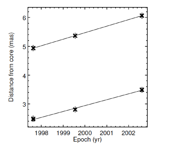
Figure 12: Proper motions of two features in the VLBA jet. The observed motions correspond to velocities of 8.1$\pm$1.2c (inner feature, bottom) and 9.4$\pm$1.2c (outer feature, top).

2.5 Comparison of X-ray and Radio Profiles

Figure 13: X-ray and radio profiles down the jet. The profile region is 2^′′ wide and 18^′′ long. The horizontal axis starts 0$\farcs$87 from the quasar and the region S2.1 is off the top scale. The heavy line is the X-ray (0.4-6 keV), the lighter line is for 5 GHz, and the dashed line is 15 GHz. The Chandra image was smoothed with a Gaussian of FWHM=0.5^′′, producing an effective resolution of about 0.85^′′. The radio maps had clean beams of 0.5^′′, but were smoothed with Gaussians suitable to produce a beam size equivalent to the Chandra resolution. The X-ray map was fractionally binned in order to match the radio pixel size of 0.05^′′.

To compare radio and X-ray structures we constructed profiles of the X-ray, 5 GHz, and 15 GHz emission of the main jet (see Figure 13). We first filtered the merged event files for the energy band 0.4-6 keV. Next we binned the data so as to match the pixel size of the radio maps. Since our event file had previously been registered so as to align the X-ray and radio nuclear positions, we employed a projection region in ds9 (Joye & Mandel, 2003) based on WCS coordinates: 2^′′ wide and 18^′′ long. We then scaled the X-ray profile by a factor of 0.01 so that both radio and X-ray curves could be easily compared. Before performing the profiles, we smoothed the X-ray data with a Gaussian of FWHM=0.5^′′ in order to minimize statistical fluctuations. For an intrinsic beam size of 0$\farcs$75, the resulting map had an effective resolution of $\approx$ 0$\farcs$85. We then applied an appropriate Gaussian smoothing to the two radio maps which originally had clean beams of 0$\farcs$5.

Within a factor of 2, the X-ray and radio profile shapes are similar, but with differences larger than those between the 5 GHz and 15 GHz profiles. For the most part, the brighter X-ray enhancements can be associated with corresponding radio knots, but not necessarily at identical positions. However, towards the end of the main jet, ($>15\arcsec\$ from the quasar), there is a marked departure: the X-ray intensities become larger going downstream whereas the radio fades away by a relative factor of 10. The overall comparison is in stark contrast to the 3C 273 jet which is X-ray bright at the upstream end, and then drops by a factor of 100 relative to the radio jet that continuously brightens going away from the quasar. For three prominent enhancements, there appears to be a small offset (of order 0$\farcs$2, or 1.4 kpc in the plane of the sky) of the peak brightness in the sense that the X-ray peaks upstream of the radio, as commonly seen in FR I jets (Hardcastle et al., 2001; Dulwich et al., 2007), and also in FR II jets, e.g., 3C353 (Kataoka et al., 2008) and quasars, e.g., PKS1127-145 (Siemiginowska et al., 2007). These knots (N to S) are located at distances 3$\farcs$9, 8$\farcs$5, and 14$\farcs$5 from the quasar. There are also jet segments for which the X-ray intensities do not track the radio. The most obvious such is the radio peak 5$\farcs$6 from the nucleus, with the X-ray peak downstream at 6$\farcs$4 in the figure. This is near the region where a galaxy overlaps the jet, and we note that the 5 GHz and 15 GHz profiles are also dissimilar there.

3 Summary

We summarize the key features of the data presented above:

• X-rays trace the radio jet along a projected length of at least 140 kpc in the plane of the sky.

• The jet is very nearly straight out to 18″ from the quasar, with an apparent projected bend of about 4° past 10″ . The intrinsic bend is probably smaller, due to the small angle of the jet to our line of sight.

• The radio and X-ray profile shapes track within a factor of 2 along the straight jet from 4″ to 14″ but cases of X-ray peaks upstream and downstream of radio peaks both occur.

• The jet appears broader in the radio than the X-ray in the region 5″ to 15″ from the core.

• The jet is at $<$ 12° to the line of sight.

• Radio and X-ray spectra are consistent with an average energy index 0.80$\pm$0.1.

• The jet likely remains relativistic far downstream of the core, as inferred from the collimation and the contraction-rarefraction structure.

• The magnetic field aligns with the jet and remains fairly uniform along the jet.

• Correlation between the total intensity and the dispersion in polarization position angle suggests that the magnetic field tends to be more turbulent in the radio knots.

• There are double hot-spots in the southern radio lobe, and separate hot spots in intensity and in polarization in the northern radio lobe. Polarization and spectral hardening indicates shock formation at the edge of the northern radio lobe.

4 Discussion and Conclusions

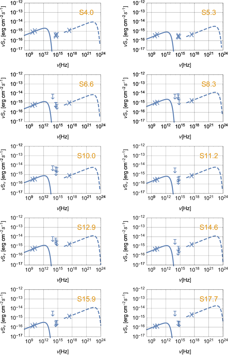
Figure 14: Inverse Compton/CMB models fit to measured radio and X-ray data, with an extrapolation giving predicted $\gamma$-ray fluxes. The models assume a power law distribution of electrons with spectral index 2.6 between $\gamma_{\rm min}$=30, and a cutoff at $\gamma_{\rm max}$=10⁵, for the entire jet. Solid lines model the radio synchrotron spectra, and dashed lines are the iC/CMB spectra from that same electron population.

We apply the iC/CMB model described by Tavecchio et al. (2000) and Celotti et al. (2001) to derive the intrinsic physical conditions of the jet. That model assumes a minimum total energy in magnetic field and relativistic particles, and requires that the jet be in relativistic motion with bulk Lorentz factor $\Gamma$ and be beamed at an angle $\theta$ to our direction with a Doppler factor $\delta=(\Gamma(1-\beta\,\cos\theta))^{-1}$. Many other assumptions are made, including that the particles and magnetic field uniformly fill the volume, that the relativistic electron spectrum dN/d$\gamma$=K$\gamma^{-m}$ gives the observed 1.4 to 15 GHz radio emission, that the charge balance is provided by protons that have equal relativistic energy as the electrons, and that the angle of the jet to our line of sight, $\theta$, takes on its maximum value for a fixed $\delta$, namely $\arcsin(1/\delta)$, so that $\delta=\Gamma$. These are the same assumptions made in Schwartz et al. (2006a), where the sensitivity to those assumed parameters was also calculated. The one difference here is that we calculate the energy in relativistic electrons by integrating from an assumed $\gamma_{\rm min}$ of the spectrum (Worrall, 2009; Schwartz et al., 2010) instead of assuming a minimum observed frequency in the radio synchrotron spectrum as originally formulated by Pacholczyk (1970). We choose $\gamma_{\rm min}$=30, consistent with the result of $\gamma_{\rm min}<80$ for PKS 0637-752 (Mueller & Schwartz, 2009). We take the volume of the regions to be cylinders of the lengths shown in Figure 1 and Table 2, and diameter assumed to be 0$\farcs$52 = 4 kpc.

Figure 14 shows the measured radio, optical, and X-ray fluxes from the 10 jet regions with detectable X-ray emission. The dashed lines model the X-ray emission as inverse Compton scattering of the cosmic microwave background, from the electrons giving rise to the synchrotron spectra shown as solid lines. We have assumed a uniform electron spectrum with index m= 2$\alpha$+1=2.6, giving a mean radiation spectrum with $\alpha$=0.80. To avoid Fermi upper limits to GeV gamma rays (Breiding et al., 2017, presented $\nu f_{\nu}<4.5\times 10^{-14}$ at $4.6\times 10^{22}$ Hz) requires a sharp cutoff to the relativistic electrons above $\gamma$=10⁵. Where optical emission is detected, from S4.0 and S5.3, it prohibits an extrapolation of the radio synchrotron spectrum to the X-ray region (Sambruna et al., 2004), as do upper limits to optical emission in regions S6.6, S8.3, S11.2, S14.6, S15.9, and S17.7. In the other regions the optical limits are too high to rule out such an extrapolation; however the radio spectrum does not directly connect to the X-rays but would over-produce the 1 keV flux density unless cut-off at a lower frequency; e.g., in regions S10.0 and S12.9.

In the iC/CMB model just sketched, we could invoke a higher cutoff to the electron spectrum to try to reproduce the optical emission. A value of $\gamma\approx$ 10^5.8 would result in the tail of the synchrotron spectrum passing close to the optical data in regions S4.0 and S5.3. The spectrum in the optical region would not be well matched, and in the absence of polarization data we do not distinguish whether such an extension or whether some additional mechanism produces the compact optical knots. The remainder of the jet would still require an upper cutoff around 10⁵ to avoid exceeding the Fermi upper limits (Breiding et al., 2017) by the summed iC/CMB from the entire jet.

As an alternative to the iC/CMB model, consider whether an additional population of electrons produces the X-ray jet via synchrotron radiation. In the jet rest frame, the magnetic field energy density equals that of the CMB when B²/(8$\pi$) = aT${}_{0}^{4}\,(1+z)^{4}\,\Gamma^{2}$. At the redshift 0.72 of 4C+19.44, the magnetic field would have to be greater than 10 $\mu$Gauss, and the jet speed would have to be less than 0.4$c$, to exceed the CMB energy density, as required for particles to emit primarily by synchrotron radiation rather than inverse Compton. In such a magnetic field, electrons emitting 1 keV synchrotron radiation would have $\gamma>$7$\times$10⁷, where we use the delta-function approximation that the particles emit at a frequency $\gamma^{2}$ times the gyro frequency. Since the synchrotron frequency depends on $\gamma^{2}$B, while the lifetime is inversely proportional to $\gamma$B², those electrons would have a lifetime less than 2300 years, or a range of less than 700 pc which projects to $<$0$\farcs$1 in the plane of the sky. By contrast, the population of 15 GHz emitting electrons would have $\gamma\approx$10⁴ and a range of 37 kpc (5″ ) in an equipartition field of $\approx$ 35 $\mu$G, where the field strength is chosen to exceed the CMB energy density even if the jet Lorentz factor were as large as $\Gamma$=4. In such a scenario it seems difficult to explain why the ratio of X-ray to radio emission remains even within a factor of 2, over a projected distance of 115 kpc, as shown in Figure 13. In a synchrotron model, the X-rays are from electrons accelerated at essentially every point in Figure 13. Some feedback mechanism must operate to coordinate the separate spectra of GHz- and X-ray- emitting electrons. The present data does not exclude such a model, subject to the constraints outlined above.

The iC/CMB model values for magnetic field strength, B, and Doppler factor, $\delta$, are presented in Figure 15. These values are of the same order as found in other one-sided kpc X-ray jets (e.g., Sambruna et al., 2002; Marshall et al., 2005; Schwartz et al., 2006a). Fixing the spectral indices at the value $\alpha$=0.80 consistent with the data, the jet shows relatively constant structure, especially from 4″ to 15″ from the quasar. In the left hand panel we use the assumption that $\Gamma=\delta$ and calculate mean values $<$B$>$ =  22 $\mu$G and $<$$\delta$$>$=7.7. The mean number density of the minimum energy electron population would be 16.5$\times$10${}^{-8}\$cm^-3, and the angle $<$$\theta$$>$=7.6° . The deprojected distance 10″ from the quasar would be 580 kpc. The kinetic power, (enthalpy flux), is calculated assuming the charge balance is provided by protons, which have total relativistic energy equal to that in the electrons. If only positrons neutralize the charge then the kinetic flux would be about 6 times less, while the magnetic field strength values would decrease by about 30%. Uncertainties in the individual quantities are 3% to 10% due to photon statistics, so systematic differences from the assumptions of isotropy of the particles and field, of uniform volume filling factor, of low energy electron cutoffs and that $\Gamma=\delta$, will dominate. In particular, past 15″ from the quasar, we calculate $\delta\approx$ 10, implying that the jet angle is moving closer to our line of sight, from a maximum of 9$.\!^{\circ}$1 to 5$.\!^{\circ}$7, if $\Gamma=\delta$. But this contradicts our empirically based hypothesis that the jet is at a constant angle to our line of sight. If we assume instead that the entire jet is at the minimum angle 5$.\!^{\circ}$7 that results from the $\Gamma=\delta$ assumption, we calculate the run of parameters shown in the right hand panel of Figure 15. The trend of magnetic field decreasing along the jet is still seen. Past 15″ the magnetic field decrease, and the concomitant decrease of the number of relativistic particles according to the minimum energy assumption, compensates for the bulk Lorentz factor increase to maintain a constant enthalpy flux at about 1$\times$10⁴⁶ erg s^-1. This could be caused by time dependent differences in the injected structure of the jet, but at constant power. Alternately , the divergence of the radio and X-ray jet profiles past 15″ may indicate a breakdown of assumptions of uniformity along the jet, or even that the iC/CMB model does not explain all the X-ray emission in this region.

We have interpreted the present results in terms of the iC/CMB model in order to estimate physical quantities in the jet. At redshifts greater than 2.5 this must be the dominant mechanism, unless the magnetic field strength is greater than 90 $\mu$G or the relativistic jet speed is less than $\beta$=0.9$c$. However, at lower redshifts the mechanism is still not certain, as has been discussed. An alternate interpretation, discussed by many authors, is to produce the X-ray and possibly optical emission by a second, high-energy electron population, as proposed e.g., for 3C 273 by Jester et al. (2006). A measurement of the spectral slope of the optical knots, extended into the infrared (e.g., by JWST), and especially measurement of the optical polarization, could indicate whether they are the extension of the electron population producing the GHz radio emission, or due to a distinct electron population as in 3C 273 (Jester et al., 2006). Significant improvement of the X-ray data for the 4C+19.44 jet would require Ms Chandra observations, which may be prohibitively expensive. More high quality multi-band data of individual jets, as well as larger samples of jets, are required to study the radiation and acceleration processes in general. Observations of high redshift X-ray jets, where we know the emission mechanism must be iC/CMB, are particularly needed. Chandra is the only X-ray observatory in at least the next twenty years which can make the required arcsec scale, high contrast observations.

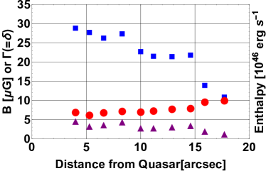
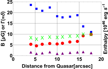
Figure 15: Left Panel: Change of the magnetic field (blue squares), Lorentz factor (red dots) and enthalpy flux (purple triangles) as a function of distance along the jet. We assume the Doppler factor equals the Lorentz factor. Right Panel: Change of the magnetic field (blue squares), Lorentz factor (red dots), Doppler factor (green crosses), and enthalpy flux (purple triangles) as a function of distance along the jet. For this calculation we assume the jet is at the constant angle $\theta$ = 5$.\!^{\circ}$8 to our line of sight. Both figures assume protons provide the charge neutrality.

References

- Alam et al. (2015) Alam, S., Albareti, F. D., Allende Prieto, C. et al. 2015 ApJS, 219, 12
- Aloy et al. (2003) Aloy, M. A., et al. 2003 ApJ, 585, 109
- Aharonian (2002) Aharonian, F. A. 2002, MNRAS, 332, 215
- Breiding et al. (2017) Breiding, P., Meyer, E. T., & Georganopoulos, M. 2017, American Astronomical Society Meeting Abstracts, 229, 250.44
- Cara et al. (2013) Cara, M., Perlman, E. S., Uchiyama, Y., et al. 2013, ApJ, 773, 2
- Celotti et al. (2001) Celotti, A., Ghisellini, G., and Chiaberge, M. 2001, MNRAS, 321, L1
- Cheung et al. (2006) Cheung, C. C., Stawarz, Ł., & Siemiginowska, A. 2006, ApJ, 650, 679
- Cheung et al. (2012) Cheung, C. C., Stawarz, Ł., Siemiginowska, A., et al. 2012, ApJ, 756, L20
- Conway & Murphy (1993) Conway, J. E., & Murphy, D. W. 1993, ApJ, 411, 89
- D’Abrusco et al. (2012) D’Abrusco, R., Massaro, F., Ajello, M. et al. 2012 ApJ, 748, 68
- Dermer (1995) Dermer, C. D. 1995, ApJ, 446, L63
- Dermer and Schlickeiser (1994) Dermer, C. D. and Schlickeiser, R. 1994, ApJS, 90, 945
- Dulwich et al. (2007) Dulwich, F., Worrall, D. M., Birkinshaw, M., Padgett, C. A., & Perlman, E. S. 2007, MNRAS, 374, 1216
- Ellingson et al. (1991) Ellingson, E., Green, R. F., & Yee, H. K. C. 1991, ApJ, 378, 476
- Freeman et al. (2001) Freeman, P., Doe, S., & Siemiginowska, A. 2001, Proc. SPIE, 4477, 76
- Ghisellini et al. (1998) Ghisellini, G., Celotti, A., Fossati, G., Maraschi, L., & Comastri, A. 1998, MNRAS, 301, 451
- Ghisellini & Celotti (2001) Ghisellini, G., & Celotti, A. 2001, MNRAS, 327, 739
- Hardcastle et al. (2001) Hardcastle, M. J., Birkinshaw, M., & Worrall, D. M. 2001, MNRAS, 326, 1499
- Hardcastle et al. (2016) Hardcastle, M. J., Lenc, E., Birkinshaw, M., et al. 2016, MNRAS, 455, 3526
- Harris and Krawczynski (2002) Harris, D. E., and Krawczynski, H. 2002,Ap.J., 565, 244
- Harris and Krawczynski (2006) Harris, D. E., and Krawczynski, H. 2006, ARAA 44, 463
- Jester et al. (2006) Jester, S., Harris, D. E., Marshall, H. L., & Meisenheimer, K. 2006, ApJ, 648, 900
- Johnston et al. (1995) Johnston, K. J., Fey, A. L., Zacharias, N., et al. 1995, AJ, 110, 880
- Joye & Mandel (2003) Joye, W. A., & Mandel, E. 2003, Astronomical Data Analysis Software and Systems XII, 295, 489
- Kataoka et al. (2008) Kataoka, J., Stawarz, Ł., Harris, D. E., et al. 2008, ApJ, 685, 839-857
- Kellermann et al. (2004) Kellermann, K. I., et al. 2004, ApJ, 609, 539
- Lister et al. (2009) Lister, M. L., Aller, H. D., Aller, M. F., et al. 2009, AJ, 137, 3718-3729
- Lucchini et al. (2017) Lucchini, M., Tavecchio,
- Marshall et al. (2005) Marshall, H. L., et al. 2005, ApJS, 156, 13
- Marshall et al. (2011) Marshall, H. L., Gelbord, J. M., Schwartz, D. A., et al. 2011, ApJS, 193, 15
- Marshall et al. (2017) Marshall, H. L., et al., submitted to ApJS
- Massaro et al. (2011) Massaro, F., Harris, D. E., & Cheung, C. C. 2011, ApJS, 197, 24
- McKeough et al. (2016) McKeough, K., Siemiginowska, A., Cheung, C. C., et al. 2016, ApJ, 833, 123
- Meyer et al. (2015) Meyer, E. T., Georganopoulos, M., Sparks, W. B., et al. 2015, ApJ, 805, 154
- Meyer et al. (2017) Meyer, E. T., Breiding, P., Georganopoulos, M., et al. 2017, ApJ, 835, L35
- Meyer & Georganopoulos (2014) Meyer, E. T., & Georganopoulos, M. 2014, ApJ, 780, L27
- Mueller & Schwartz (2009) Mueller, M., & Schwartz, D. A. 2009, ApJ, 693, 648
- Pacholczyk (1970) Pacholczyk, A. G. 1970, Series of Books in Astronomy and Astrophysics, San Francisco: Freeman, 1970
- Perlman et al. (2001) Perlman, E. S., Biretta, J. A., Sparks, W. B., Macchetto, F. D., & Leahy, J. P. 2001, ApJ, 551, 206
- Perlman et al. (2011) Perlman, E. S., Georganopoulos, M., Marshall, H. L., et al. 2011, ApJ, 739, 65
- Ryabinkov, Kaminker, & Varshalovich (2003) Ryabinkov, A. I., Kaminker, A. D.& Varshalovich, D. A. 2003 A&A 412, 707
- Sambruna et al. (2002) Sambruna, R. M., Maraschi, L., Tavecchio, F., Urry, C. M., Cheung, C. C., Chartas, G., Scarpa, R., & Gambill, J. K. 2002, ApJ, 571, 206
- Sambruna et al. (2004) Sambruna, R. M., Gambill, J.K., Maraschi, L., Tavecchio, F., Cerutti, R., Cheung, C. C., Urry, C. M., & Chartas, G., 2004, ApJ, 608, 698
- Sambruna et al. (2006) Sambruna, R. M., Gliozzi, M., Donato, D., et al. 2006, ApJ, 641, 717
- Schneider et al. (2010) Schneider, D. P., Richards, G. T., Hall, P. B., et al. 2010, AJ, 139, 2360
- Schwartz et al. (2000) Schwartz, D. A., et al. 2000,ApJ, 540, L69
- Schwartz (2002) Schwartz, D. A. 2002, ApJ, 569, L23
- Schwartz et al. (2006a) Schwartz, D. A., et al. 2006a, ApJ, 640, 592
- Schwartz et al. (2006b) Schwartz, D. A., Marshall, H. L., Lovell, J. E. J., et al. 2006b, ApJ, 647, L107
- Schwartz et al. (2007a) Schwartz, D. A., Harris, D. E., Landt, H., et al. 2007a, Ap&SS, 311, 341
- Schwartz et al. (2007b) Schwartz, D. A., Harris, D. E., Landt, H., et al. 2007b, Proc. IAU Symp. No. 238 Black Holes from Stars to Galaxies – Across the Range of Masses, 238, 443
- Schwartz et al. (2010) Schwartz, D. A., Massaro, F., Siemiginowska, A., et al. 2010, International Journal of Modern Physics D, 19, 879
- Schwartz et al. (2015) Schwartz, D. A., Marshall, H. L., Worrall, D. M., et al. 2015, Extragalactic Jets from Every Angle, IAU Symposium 313, 219
- Siemiginowska et al. (2002) Siemiginowska, A, Bechtold, J., Aldcroft, T. L., Elvis, M., Harris, D. E., Dobrzycki, A. 2002, ApJ, 570, 543
- Siemiginowska et al. (2003b) Siemiginowska, A., Smith, R. K., Aldcroft, T. L., Schwartz, D. A., Paerels, F., & Petric, A. O. 2003, ApJ, 598, L15
- Siemiginowska et al. (2007) Siemiginowska, A., Stawarz, Ł., Cheung, C. C., et al. 2007, ApJ, 657, 145
- Siemiginowska et al. (2010) Siemiginowska, A., Burke, D. J., Aldcroft, T. L., Worrall, D. M., Allen, S., Bechtold, J., Clarke, T., & Cheung, C. C. 2010, ApJ, 722, 102
- Simard-Normandin et al. (1981) Simard-Normandin, M., Kronberg, P. P., & Button, S. 1981, ApJS, 45, 97
- Simionescu et al. (2016) Simionescu, A., Stawarz, Ł., Ichinohe, Y., et al. 2016, ApJ, 816, L15
- Singal (2016) Singal, A. K. 2016, ApJ, 827, 66
- Steidel & Sargent (1991) Steidel, C. C., & Sargent, W. L. W. 1991, ApJ, 382, 433
- Tavecchio et al. (2000) Tavecchio, F.,Maraschi, L., Sambruna, R. M., Urry, C. M. 2000, ApJ, 544, L23
- Uchiyama et al. (2006) Uchiyama, Y., Urry, C. M., Cheung, C. C., Jester, S., Van Duyne, J., Coppi, P., Sambruna, R. M., Takahashi, T., Tavecchio, F., & Maraschi, L. 2006, ApJ, 648, 910
- Wilson et al. (2000) Wilson, A.S., Young, A.J., and Shopbell,P.L., 2000, Ap.J., 544, L27
- Wilson et al. (2001) Wilson, A. S., Young, A. J., & Shopbell, P. L. 2001, Particles and Fields in Radio Galaxies, ASP Conf. Series 250, 213
- Worrall (2009) Worrall, D. M. 2009, A&A Rev., 17, 1
- Worrall et al. (2001) Worrall, D. M., Birkinshaw, M., & Hardcastle, M. J. 2001, MNRAS, 326, L7
- Zensus et al. (2002) Zensus, J. A., Ros, E., Kellermann, K. I., Cohen, M. H., Vermeulen, R. C., & Kadler, M. 2002, AJ, 124, 662