The Polymorphic Evolution Sequence for Populations with Phenotypic Plasticity

Abstract.

In this paper we study a class of stochastic individual-based models that describe the evolution of haploid populations where each individual is characterised by a phenotype and a genotype. The phenotype of an individual determines its natural birth- and death rates as well as the competition kernel, $c(x,y)$ which describes the induced death rate that an individual of type $x$ experiences due to the presence of an individual or type $y$. When a new individual is born, with a small probability a mutation occurs, i.e. the offspring has different genotype as the parent. The novel aspect of the models we study is that an individual with a given genotype may express a certain set of different phenotypes, and during its lifetime it may switch between different phenotypes, with rates that are much larger then the mutation rates and that, moreover, may depend on the state of the entire population. The evolution of the population is described by a continuous-time, measure-valued Markov process. In [4], such a model was proposed to describe tumor evolution under immunotherapy. In the present paper we consider a large class of models which comprises the example studied in [4] and analyse their scaling limits as the population size tends to infinity and the mutation rate tends to zero. Under suitable assumptions, we prove convergence to a Markov jump process that is a generalisation of the polymorphic evolution sequence (PES) as analysed in [8, 10].

1. Introduction

Over the last decade there has been increasing interest in the mathematical analysis of so-called stochastic individual based models of adaptive dynamics. These models were introduced in a series of papers by Bolker, Pacala, Dieckmann, and Law [6, 7, 12]. They describe the evolution of a population of individuals characterised by their phenotypes under the influence of the evolutionary mechanisms of birth, death, mutation, and ecological competition in an inhomogeneous "fitness landscape" as a measure valued Markov process. In these models there appear two natural scaling parameters. The carrying capacity, $K$, which regulates the size of the population and that can reasonably considered as a large parameter, and the mutation rate (of advantageous mutations), $u$, that in many biological situations can be taken as a small parameter. In a series of remarkable papers, Champagnat and Méléard [8, 10] (and others) have analysed the limiting processes that arise in the limit when $K$ is taken to infinity while at the same time $u=u_{K}$ tends to zero. Under conditions that ensure the separation of the ecological and evolutionary time scales. This means that the mutation rates are so small that the system has time to equilibrate (ecological time scale) between two mutational events. On the time scale where mutations occur (evolutionary time scale), the evolution of the population can then be described as a Markov jump process along a sequence of equilibria of, in general, polymorphic populations. An important (and in some sense generic) special case occurs when the mutant population fixates while the resident population dies out in each step. The corresponding jump process is called the Trait Substitution Sequence (TSS) in adaptive dynamics. Champagnat [8] derived criteria in the context of individual-based models under which convergence to the TSS can be proven. The general process is called the Polymorphic Evolution Sequence (PES) [10]. Here the limit is describes as a jump process between possibly polymorphic equilibria of systems of Lotka-Volterra equations of increasing dimension.

In the present paper we extend this analysis to models where an additional biological phenomenon is present, the so-called phenotypic plasticity. By this we mean the following. Individuals are no longer described by their phenotype, but by both their genotype and their phenotype. Moreover, an individual of a given phenotype can express several phenotypes and it can change its phenotype during the course of its lifetime.

Our original motivation for this comes from applications to cancer therapy, where it is well-known that phenotypic switches (“phenotypic plasticity") is of utmost importance and in fact a major obstacle to successful therapies (see, e.g. [17] and references therein). For a first attempt at modelling specific scenarios in the framework of individual based stochastic models, see [4]. However, phenotypic switches without mutations are certainly relevant in many if not most biological systems.

Here we take a broader look at a large class of models. By expanding the techniques of [10] we prove that the microscopic process converges on the evolutionary time scale to a generalisation of the Polymorphic Evolution Sequences (PES) (cf. Thm. 3.3). The main difference in the proof is that we have to couple the process with multi-type branching processes instead of normal branching processes, which leads also to a different definition of invasion fitness in this setting. Note that we gave in [4] already heuristic arguments why the process should converge to a Markov jump process. The aim of this paper is to give the rigorous statement and its proof.

The remainder of this paper is organised as follows. In Section 2 we define the model, give a pathwise description of the Markov process we are studying and state the convergence towards a quadratic system of ODEs in the large population limit. In Sections 3 we consider the case of rare mutations and fast switches. More precisely, we state the convergence to the Polymorphic Evolution Sequences with phenotypic Plasticity (PESP) in Subsection 3.2 and prove it in Subsection 3.3.

2. The microscopic model

In this section we introduce the stochastic individual-based model we analyse (cf. [4, 15, 8, 10, 5]). The evolutionary process changes populations on a macroscopic level, but the basic mechanisms of evolution, heredity, variation (in our context caused by mutation and phenotypical switching), and selection, act on the microscopic level of the individuals. We describe the evolving population as a stochastic system of interacting individuals, where each individual is characterised by its phenotype and its genotype.

Let $l\geq 1$ and $\mathcal{X}$ a finite set of the form $\mathcal{X}=\mathcal{G}\times\mathcal{P}$, where $\mathcal{G}$ is the set of genotypes and $\mathcal{P}$ is the set of phenotypes. We call $\mathcal{X}$ the trait space of the population. As usual, we introduce a parameter $K\in\mathbb{N}$, called the carrying capacity. This parameter allows to scale the population size and can be interpreted as the size of available space or the amount of available resources. Let $\mathcal{M}(\mathcal{X})$ be the set of finite, non-negative measures on $\mathcal{X}$, equipped with the topology of weak convergence, and let $\mathcal{M}^{K}(\mathcal{X})\subset\mathcal{M}(\mathcal{X})$ be the set of finite point measures on $\mathcal{X}$ rescaled by K, i.e.

$$\mathcal{M}^{K}(\mathcal{X})\equiv\left\{\frac{1}{K}\sum_{i=1}^{n}\delta_{x_{i}}\>:\>n\in{\mathbb{N}}_{0},\>x_{1},\ldots x_{n}\in\mathcal{X}\right\},$$ (2.1)

where $\delta_{x}$ denotes the Dirac mass at $x\in\mathcal{X}$. We model the time evolution of a population as an $\mathcal{M}^{K}(\mathcal{X})$-valued, continuous time Markov process $(\nu^{K}_{t})_{t\geq 0}$. To account for the process basic mechanisms of evolution and the phenotypic plasticity, we introduce the following parameters:

1. $b(p)\in\mathbb{R}_{+}$ is the rate of birth of an individual with phenotype $p\in\mathcal{P}$.

2. $d(p)\in\mathbb{R}_{+}$ is the rate of natural death of an individual with with phenotype $p\in\mathcal{P}$.

3. $c(p,\tilde{p})K^{-1}\in\mathbb{R}_{+}$ is the competition kernel which models the competitive pressure an individual with phenotype $p\in\mathcal{P}$ feels from an individual with phenotype $\tilde{p}\in\mathcal{P}$ and is inversely proportional to the carrying capacity $K$.

4. $s_{\text{nat.}}^{g}(p,\tilde{p})\in{\mathbb{R}}_{+}$ is the natural switch kernel which models the natural switching from phenotype $p$ to $\tilde{p}$ of individuals with genotype $g$.

5. $s_{\text{ind.}}^{g}(p,\tilde{p})(\hat{p})K^{-1}\in\mathbb{R}_{+}$ is the induced switch kernel which models the switching from phenotype $p$ to $\tilde{p}$ of individuals with genotype $g$ induced by an individual with phenotype $\hat{p}$.

   (Compare with the cytokine-induced switch of [4], especially the one of TNF-${\alpha}$ (Tumour Necrosis Factor).)

6. $u_{K}m(g)$ with $u_{K},m(g)\in[0,1]$ is the probability that a mutation occurs at birth from an individual with genotype $g\in\mathcal{G}$, where $u_{K}$ is a scaling parameter.

7. $M((g,p),(\tilde{g},\tilde{p}))$ is the mutation law, i.e. if a mutant is born from an individual with trait $(g,p)$, then the mutant’s trait is $(\tilde{g},\tilde{p})$ with probability $M((g,p),(\tilde{g},\tilde{p}))$.

Note that most of the parameters depend on the phenotype only and that we explicitly allow that individuals with different genotypes can express the same phenotype and conversely that individuals with the same genotype can express different phenotypes.

Assumption 1.

For simplicity we assume that $s_{\text{ind.}}^{g}(p,\tilde{p})(\hat{p})K^{-1}=0$ for all $\hat{p}\in\mathcal{X}$ whenever $s_{\text{nat.}}^{g}(p,\tilde{p})=0$, i.e. depending on the environment the total switching rate can be larger or smaller but not zero or non-zero.

At any time $t\geq 0$, we consider a finite population which consist of $N_{t}$ individuals and each individual is characterised its trait $x_{i}(t)\in\mathcal{X}$. The state of a population at time $t$ is the measure

$$\nu^{K}_{t}=\frac{1}{K}\sum_{i=1}^{N_{t}}\delta_{x_{i}(t)}.$$ (2.2)

The population process $\nu^{K}$ is a $\mathcal{M}^{K}(\mathcal{X})$-valued Markov process with infinitesimal generator ${\mathscr{L}^{K}}$, defined, for any bounded measurable function $\phi:\mathcal{M}^{K}(\mathcal{X})\rightarrow\mathbb{R}$ and for all $\mu^{K}\in\mathcal{M}^{K}(\mathcal{X})$ by

$$\left({\mathscr{L}^{K}}\phi\right)(\mu^{K})$$ (2.3)

$$\>=\sum_{(g,p)\in\mathcal{G}\times\mathcal{P}}\left(\phi\left(\mu^{K}+\tfrac{\delta_{(g,p)}}{K}\right)-\phi(\mu^{K})\right)(1-u_{K}m(g))b(p)K\mu^{K}(g,p)$$

$$\quad+\sum_{(g,p)\in\mathcal{G}\times\mathcal{P}}\sum_{(\tilde{g},\tilde{p})\in\mathcal{G}\times\mathcal{P}}\left(\phi\left(\mu^{K}+\tfrac{\delta_{(\tilde{g},\tilde{p})}}{K}\right)-\phi(\mu^{K})\right)u_{K}m(g)M\big{(}(g,p),(\tilde{g},\tilde{p})\big{)}b(p)K\mu^{K}(g,p)$$

$$\quad+\sum_{(g,p)\in\mathcal{G}\times\mathcal{P}}\left(\phi\left(\mu^{K}-\tfrac{\delta_{(g,p)}}{K}\right)-\phi(\mu^{K})\right)\biggl{(}d(p)+\sum_{\tilde{p}\in\mathcal{P}}c(p,\tilde{p})\mu^{K}(\tilde{p})\biggr{)}K\mu^{K}(g,p)$$

$$\quad+\sum_{(g,p)\in\mathcal{G}\times\mathcal{P}}\>\sum_{\tilde{p}\in\mathcal{P}}\left(\phi\left(\mu^{K}+\tfrac{\delta_{(g,\tilde{p})}}{K}-\tfrac{\delta_{(g,p)}}{K}\right)-\phi(\mu^{K})\right)\biggl{(}s_{\text{nat.}}^{g}(p,\tilde{p})+\sum_{\hat{p}\in\mathcal{P}}s^{g}_{\text{ind.}}(p,\tilde{p})(\hat{p})\mu^{K}(\hat{p})\biggr{)}\>K\mu^{K}(g,p).$$

The first and second terms describe the births (without and with mutation), the third term describes the deaths due to age or competition, and the last term describes the phenotypic plasticity. Observe that the first and second terms are linear (in $\mu^{K}$ ), but the third and fourth terms are non-linear. The only difference to the standard model is the presence of the fourth term that corresponds to the phenotypic switches. However, this term changes the dynamics substantially. In particular, the system of differential equations which arises in the large population limit without mutation ($u_{K}=0$) is not a generalised Lotka-Volterra system anymore, i.e. has not the form $\dot{\mathfrak{n}}=\mathfrak{n}f(\mathfrak{n})$, where $f$ is linear in $\mathfrak{n}$ (cf. Thm. 2.1 and Def. 3.1).

Remark 1.

1. Since $\mathcal{X}$ is finite, we could also represent the population state as an $|\mathcal{X}|$-dimensional vector. More precisely, let $E$ be a subset of $\mathbb{R}^{|\mathcal{X}|}$ and $E^{K}\equiv E\cup\{n/K:n\in\mathbb{N}_{0}\}$, then for fixed $K\geq 1$, the population process can be constructed as Markov process with state space $E^{K}$ by using independent standard Poisson processes (cf. [14] Chap. 11).

2. For an extension to a non-finite trait space, e.g. if $\mathcal{G}$ and $\mathcal{P}$ are compact subsets of $\mathbb{R}^{k}$ for some $k\geq 1$, the modeling of switching the phenotype has to be changed in the following way: Each individual with trait $(g,p)\in\mathcal{G}\times\mathcal{P}$ has instead of the natural switch kernel $s_{\text{nat.}}^{g}(p,\tilde{p})$ a natural switch rate $s_{\text{nat.}}(g,p)$ combined with a probability measure ${S}_{\text{nat.}}^{(g,p)}(d\tilde{p})$ on $\mathcal{P}$ and instead of the induced switch kernel $s_{\text{ind.}}^{g}(p,\tilde{p})(\hat{p})K^{-1}$ a induced switch kernel $s_{\text{ind.}}((g,p),\hat{p})K^{-1}$ combined with a family of probability measure $\{{S}_{\text{ind.}}^{((g,p),\hat{p})}(d\tilde{p})\}$ on $\mathcal{P}$.

2.1. Explicit construction of the population process with phenotypic plasticity

It is useful to give a pathwise description of $\nu^{K}$ in terms of Poisson point measures (cf. [15]). Let us recall this construction. Let $(\Omega,\mathcal{F},\mathbb{P})$ be an abstract probability space. On this space, we define the following independent random elements:

1. a convergent sequence $(\nu^{K}_{0})_{K\geq 1}$ of $\mathcal{M}^{K}(\mathcal{X})$-valued random measures (the random initial population),

2. $|\mathcal{X}|$ independent Poisson point measures $(\,N^{\text{birth}}_{(g,p)}(ds,di,d\theta)\,)_{(g,p)\in\mathcal{X}}$ on $\,[0,\infty)\times\mathbb{N}\times\mathbb{R}_{+}\,$ with intensity measure $ds\sum_{n\geq 0}\delta_{n}(di)d\theta$,

3. $|\mathcal{X}|$ independent Poisson point measures $(\,N^{\text{mut.}}_{(g,p)}(ds,di,d\theta,dx)\,)_{(g,p)\in\mathcal{X}}$ on $\,[0,\infty)\times\mathbb{N}\times\mathbb{R}_{+}\times\mathcal{X}\,$ with intensity measure $\,ds\sum_{n\geq 0}\delta_{n}(di)d\theta\sum_{\tilde{x}\in\mathcal{X}}\delta_{\tilde{x}}(dx)$.

4. $|\mathcal{X}|$ independent Poisson point measures $(\,N^{\text{death}}_{(g,p)}(ds,di,d\theta)\,)_{(g,p)\in\mathcal{X}}$ on $\,[0,\infty)\times\mathbb{N}\times\mathbb{R}_{+}\,$ with intensity measure $\,ds\sum_{n\geq 0}\delta_{n}(di)d\theta$,

5. $|\mathcal{X}|$ independent Poisson point measures $(\,N^{\text{switch}}_{(g,p)}(ds,di,d\theta,dp)\,)_{(g,p)\in\mathcal{X}}$ on $\,[0,\infty)\times\mathbb{N}\times\mathbb{R}_{+}\times\mathcal{P}\,$ with intensity measure $\,ds\sum_{n\geq 0}\delta_{n}(di)d\theta\sum_{\tilde{p}\in\mathcal{P}}\delta_{\tilde{p}}(dp)$,

Then, $\nu^{K}$ is given by the following equation

$$\nu_{t}^{K}=\> \nu_{0}^{K}+\!\sum_{(g,p)\in\mathcal{X}}\int_{0}^{t}\int_{\mathbb{N}_{0}}\int_{\mathbb{R}_{+}}\mathds{1}_{\left\{i\leq K\nu^{K}_{s-}(g,p),\;\theta\leq b(p)\left(1-u_{K}m(g)\right)\right\}}\tfrac{1}{K}{{\delta}_{(g,p)}}N^{\text{birth}}_{(g,p)}(ds,di,d{\theta})$$ (2.4)

$$+\sum_{(g,p)\in\mathcal{X}}\int_{0}^{t}\int_{\mathbb{N}_{0}}\int_{\mathbb{R}_{+}}\int_{\mathcal{X}}\mathds{1}_{\left\{i\leq K\nu^{K}_{s-}(g,p),\;\theta\leq b(p)u_{K}m(g)M((g,p),x)\right\}}\tfrac{1}{K}{{\delta}_{x}}N_{(g,p)}^{\text{mut.}}(ds,di,d{\theta},dx)$$

$$-\sum_{(g,p)\in\mathcal{X}}\int_{0}^{t}\int_{\mathbb{N}_{0}}\int_{\mathbb{R}_{+}}\mathds{1}_{\left\{i\leq K\nu^{K}_{s-}(g,p),\;\theta\leq d(p)+\sum_{\tilde{p}\in\mathcal{P}}c(p,\tilde{p})\nu^{K}_{s^{-}}(\tilde{p})\right\}}\tfrac{1}{K}{{\delta}_{(g,p)}}N_{(g,p)}^{\text{death}}(ds,di,d{\theta})$$

$$+\sum_{(g,p)\in\mathcal{X}}\int_{0}^{t}\int_{\mathbb{N}_{0}}\int_{\mathbb{R}_{+}}\int_{\mathcal{P}}{\mathds{1}_{\left\{i\leq K\nu^{K}_{s-}(g,p),\;\theta\leq s_{\text{nat.}}^{g}(p,\tilde{p})+\sum_{\hat{p}\in\mathcal{P}}s^{g}_{\text{ind.}}(p,\tilde{p})(\hat{p})\nu_{s-}^{K}(\hat{p})\right\}}}$$

$$\hskip 170.71652pt\times\tfrac{1}{K}\left({{\delta}_{(g,\tilde{p})}-{\delta}_{(g,p)}}\right)N_{(g,p)}^{\text{switch}}(ds,di,d{\theta},d\tilde{p}).$$

Remark 2.

This construction uses that $\mathcal{X}$ is a discrete set and is in some sense closer to the definition given in [14] (p. 455). For non-discrete trait spaces the process can be constructed as in [15].

2.2. The Law of Large Numbers.

If the mutation rate is independent of $K$ and the initial conditions converge to a deterministic limit, then the sequence of rescaled processes, $(\nu^{K})_{K\geq 1}$, converges, almost surely, as $K\uparrow\infty$ to the solution of system of ODEs. This follows directly from the law of large numbers for density depending processes, see, e.g. Ethier and Kurtz [14], Chap. 11. The following theorem gives a precise statement.

Theorem 2.1.

Let $u_{K}\equiv{1}$. Suppose that the initial conditions converge almost surely to a deterministic limit, i.e. $\lim_{K\uparrow\infty}\nu^{K}_{0}=\nu_{0}$, where $\nu_{0}$ is a finite measure on $\mathcal{X}$. Then, for every $T>0$, exists a deterministic function $\xi\in C([0,T],\mathcal{M}_{F}(\mathcal{X}))$ such that

$$\lim_{K\uparrow\infty}\sup_{t\in[0,T]}\big{|}\big{|}\nu^{K}_{t}-\xi_{t}\big{|}\big{|}_{\text{TV}}=0,\qquad\text{a.s.,}$$ (2.5)

where $||\,.\,||{}_{\text{TV}}$ is the total variation norm. Moreover, let $\mathfrak{n}$ be the unique solution to the dynamical system

$$\quad\dot{\mathfrak{n}}_{(g,p)}(t)\>= \;\mathfrak{n}_{(g,p)}(t)\>\Biggl{(}\bigl{(}1-m(g)\bigr{)}b(p)-d(p)-\sum_{(\tilde{g},\tilde{p})\in\mathcal{G}\times\mathcal{P}}c(p,\tilde{p})\mathfrak{n}_{(\tilde{g},\tilde{p})}(t)$$ (2.6)

$$\hskip 71.13188pt-\sum_{\tilde{p}\in\mathcal{P}}\biggl{(}s_{\text{nat.}}^{g}(p,\tilde{p})+\sum_{(\hat{g},\hat{p})\in\mathcal{G}\times\mathcal{P}}s^{g}_{\text{ind.}}(p,\tilde{p})(\hat{p})\mathfrak{n}_{(\hat{g},\hat{p})}(t)\biggr{)}\Biggr{)}$$

$$+\quad\sum_{\tilde{p}\in\mathcal{P}}\;\;\mathfrak{n}_{(g,\tilde{p})}(t)\>\biggl{(}s_{\text{nat.}}^{g}(\tilde{p},p)+\sum_{(\hat{g},\hat{p})\in\mathcal{G}\times\mathcal{P}}s^{g}_{\text{ind.}}(\tilde{p},p)(\hat{p})\mathfrak{n}_{(\hat{g},\hat{p})}(t)\biggr{)}$$

$$+\sum_{(\tilde{g},\tilde{p})\in\mathcal{G}\times\mathcal{P}}\mathfrak{n}_{(\tilde{g},\tilde{p})}(t)\>m(\tilde{g})b(\tilde{p})M((\tilde{g},\tilde{p}),(g,p)),\quad(g,p)\in\mathcal{G}\times\mathcal{P},$$

with initial condition $\mathfrak{n}_{x}(0)=\nu_{0}(x)$ for all $x\in\mathcal{X}$.
Then, $\xi$ is given as $\xi_{t}=\sum_{x\in\mathcal{X}}\mathfrak{n}_{x}(t)\delta_{x}$.

Proof.

This result follows from Theorem 2.1 in Chapter 11 of [14], since we can construct the process as described in Remark 1 (i). For more details see [21]. ∎

Remark 3.

If the trait spaces is not finite, one can obtain a similar result, cf. [15].

3. The interplay between rare mutations and fast switches.

In this section we state our main results. As in previous work, we place ourselves under the assumptions

$$\forall V>0,\qquad\exp(-VK)\ll u_{K}\ll\frac{1}{K\ln K},\qquad\text{as }K\uparrow\infty,$$ (3.1)

which ensure that a population reaches equilibrium before a new mutant appears. Under these assumptions we prove that the individual-based process with phenotypic plasticity convergences to a generalisation of the PES. Let us start with describing the techniques used in [10].

The key element in the proof of the convergence to the PES used by Champagnat and Méléard [10] is a precise analysis of how a mutant population fixates. A crucial assumption in [10] is that the competitive Lotka-Volterra systems that describes the large population limit always have a unique stable fixed point $\bar{\mathfrak{n}}$. Thus, the main task is to study the invasion of a mutant that has just appeared in a population close to equilibrium. The invasion can be divided into three steps: First, as long as the mutant population size is smaller than $K\epsilon$, for a fixed small $\epsilon>0$, the resident population stays close to its equilibrium. Therefore, the mutant population can be approximated by a branching process. Second, once the mutant population reaches the level $K\epsilon$, the whole system is close to the solution of the corresponding deterministic system and reaches an $\epsilon$-neighbourhood of $\bar{\mathfrak{n}}$ in finite time. Third, the subpopulations which have a zero coordinate in $\bar{\mathfrak{n}}$ can be approximated by subcritical branching processes until they die out.

The first and third steps require a time of order $\ln(K)$, whereas the second step requires only a time of order one, independent of $K$. Since the expected time between two mutations is of order $1/(u_{K}K)$, the the upper bound on $u_{K}$ in (3.1) guarantees that, with high probability, the three steps of an invasion are completed before a new mutation occurs.

In the first invasion step the invasion fitness of a mutant plays a crucial role. Given a population in a stable equilibrium that populates a certain set of traits, say $M\subset\mathcal{X}$, the invasion fitness $f(x,M)$ is the growth rate of a population consisting of a single individual with trait $x\not\in M$ in the presence of the equilibrium population $\bar{\mathfrak{n}}$ on $M$. In the case of the standard model, it is given by

$$f(x,M)=b(x)-d(x)-\sum_{y\in M}c(x,y)\bar{\mathfrak{n}}_{y}.$$ (3.2)

Positive $f(x,M)$ implies that a mutant appearing with trait $x$ from the equilibrium population on $M$ has a positive probability (uniformly in $K$) to grow to a population of size of order $K$; negative invasion fitness implies that such a mutant population will die out with probability tending to one (as $K\uparrow\infty$) before it can reach a size of order $K$. The reason for this is that the branching process (birth-death process) which approximates the mutant population is supercritical if $f(x,M)$ is positive and subcritical if $f(x,M)$ is negative.

In order to describe the dynamics of a phenotypically heterogeneous population on the evolutionary time scale, we have to adapt the notion of invasion fitness to the case where fast phenotypic switches are present. Since switches between phenotypes associated to the same genotype happen at times of order one, the growth rate of the initial mutant phenotype does not determine the probability of fixation. See [11] for a similar issue in a model with sexual reproduction. In the proof of Theorem 3.3 we approximate the dynamics of the mutant population by a multi-type branching process until the reaches a size $K\epsilon$ (or dies out). A continuous-time multi-type branching process is supercritical if and only if the largest eigenvalue of its infinitesimal generator of is strictly positive (cf. [2, 23]). Therefore, this eigenvalue will provide an appropriate generalisation of the invasion fitness.

3.1. The competitive Lotka-Volterra system with phenotypic plasticity.

We first consider the large population limit without mutation $(u_{K}\equiv 0)$. Assume tha the initial condition is supported on $d$ traits, $(\mathbf{g},\mathbf{p})=((g_{1},p_{1}),\ldots,(g_{d},p_{d}))\in(\mathcal{G}\times\mathcal{P})^{d}$, and that the sequence of the initial conditions converges almost surely to a deterministic limit, i.e.

$$\lim_{K\uparrow\infty}\nu_{0}^{K}=\sum_{i=1}^{d}n_{i}(0)\delta_{(g_{i},p_{i})},\quad\text{a.s.,}\qquad\text{ where $n_{i}(0)>0$ for all $i\in\{1\ldots d\}$. }$$ (3.3)

By Theorem 2.1, for every $T>0$, the sequences of processes $\nu^{K}\in\mathbb{D}([0,T],\mathcal{M}^{K}(\mathcal{X}))$ generated by ${\mathscr{L}}^{K}$ with initial state $\nu_{0}^{K}$ converges almost surely, as $K\uparrow\infty$, to a deterministic function $\xi\in C([0,T],\mathcal{M}(\mathcal{X}))$. Since $u_{K}\equiv 0$, no new genotype can appear in the population process $\nu^{K}$. Moreover, not every genotype can express every phenotype. <let us describe the support of $\nu_{t}^{K}$ more precisely.

For all $g\in\mathcal{G}$, let $X^{g}$ be a stationary discrete-time Markov chain with state space $\mathcal{P}$ and transition probabilities

$$\mathbb{P}[X^{g}_{i}=\tilde{p}\>|\>X^{g}_{i-1}=p]=\frac{s^{g}(p,\tilde{p})}{\sum_{\hat{p}\in\mathcal{P}}s^{g}(p,\hat{p})},\quad\text{ if }\sum_{\hat{p}\in\mathcal{P}}s^{g}(p,\hat{p})>0$$ (3.4)

and

$$\mathbb{P}[X^{g}_{i}=p\>|\>X^{g}_{i-1}=p]=1,\quad\text{ if }\sum_{\hat{p}\in\mathcal{P}}s^{g}(p,\hat{p})=0.$$ (3.5)

The Markov chains $\{X^{g},g\in\mathcal{G}\}$ contain only partial information on the switching behaviour of the process $\nu^{K}$, but we see that this is the key information needed later.

In the sequel we work under the following simplifying assumption:

Assumption 2.

For all $g\in\mathcal{G}$, all communicating classes of $X^{g}$ are recurrent.

We denote the communicating class associated with $(g,p)\in\mathcal{G}\times\mathcal{P}$ by $[p]_{g}$. This is the communicating class of $X^{g}$ which contains $p$, i.e. $p$ can be seen as a representative of the class, which has an equivalence relation depending on $g$.

Figure 1. Example of a Markov chain $X^{g}$. Here, $\mathcal{P}=\{p_{1},\ldots,p_{10}\}$ and $X^{g}$ has four communicating classes: $\{p_{1},p_{2},p_{3},p_{4}\},\{p_{5},p_{6},p_{7}\},\{p_{8}\},\{p_{9},p_{10}\}$. The class $\{p_{8}\}$ has only one element, i.e. $\sum_{i=1}^{10}s^{g}(p_{8},p_{i})=0$ in this example.

By Assumption 1, this ensures that if we start with a large enough population consisting only of individuals carrying the same trait $(g,p)$, then, after a short time, all phenotypes in the class $[p]_{g}$ will be present in the population, but none of the other classes. Observe that these Markov chains do not describe the dynamics of the whole process. If we allowed transient states this would not imply that the trait would get extinct, since its growth rate could be larger than the switching rate.

Thus, $[p]_{g}$ is the set of phenotypes which are reachable in the Markov chain $X^{g}$ with $X^{g}_{0}=p$ and the set of traits which can appear in the population process $\nu^{K}$ is given by

$$\mathcal{X}_{(\mathbf{g},\mathbf{p})}\equiv\bigcup_{i=1}^{d}\{g_{i}\}\times[p_{i}]_{g_{i}}.$$ (3.6)

With this notation, $\xi$ is given by $\xi(t)=\sum_{x\in\mathcal{X}_{(\mathbf{g},\mathbf{p})}}{\mathfrak{n}}_{x}(t)\delta_{x}$, where ${\mathfrak{n}}$ is the solution of the competitive Lotka-Volterra system with phenotypic plasticity defined below.

Definition 3.1.

For any $(\mathbf{g},\mathbf{p})\in(\mathcal{G}\times\mathcal{P})^{d}$, we denote by $LVS(d,(\mathbf{g},\mathbf{p}))$ the competitive Lotka-Volterra system with phenotypic plasticity. This is an $|\mathcal{X}_{(\mathbf{g},\mathbf{p})}|$-dimensional system of ODEs given by

$$\dot{{\mathfrak{n}}}_{(g,p)}=\> \mathfrak{n}_{(g,p)}\biggl{(}b(p)-d(p)-\!\!\sum_{(\tilde{g},\tilde{p})\in\mathcal{X}_{(\mathbf{g},\mathbf{p})}}\!\!c(p,\tilde{p})\mathfrak{n}_{(\tilde{g},\tilde{p})}-\!\!\sum_{\tilde{p}\in[p]_{g}}\biggl{(}s_{\text{nat.}}^{g}(p,\tilde{p})+\!\!\sum_{(\hat{g},\hat{p})\in\mathcal{X}_{(\mathbf{g},\mathbf{p})}}\!\!s^{g}_{\text{ind.}}(p,\tilde{p})(\hat{p})\mathfrak{n}_{(\hat{g},\hat{p})}(t)\biggr{)}\biggr{)}$$

$$+\!\!\sum_{\tilde{p}\in[p]_{g}}\mathfrak{n}_{(g,\tilde{p})}\biggl{(}s_{\text{nat.}}^{g}(\tilde{p},p)+\!\!\sum_{(\hat{g},\hat{p})\in\mathcal{X}_{(\mathbf{g},\mathbf{p})}}\!\!s^{g}_{\text{ind.}}(\tilde{p},p)(\hat{p})\mathfrak{n}_{(\hat{g},\hat{p})}(t)\biggr{)},\quad(g,p)\in\mathcal{X}_{(\mathbf{g},\mathbf{p})}.$$ (3.7)

We choose the (possibly misleading) name competitive Lotka-Volterra system with phenotypic plasticity to emphasise that we add phenotypic plasticity (induced by switching rates) in the usual competitive Lotka-Volterra system. Note, however, that the system $LVS$ is not a system of Lotka-Volterra equations.

We now introduce the notation of coexisting traits in this context (cf. [10]).

Definition 3.2.

For any $d\geq 2$, we say that the distinct traits $(g_{1},p_{1}),\ldots,(g_{d},p_{d})$ coexist if the system $LVS(d,(\mathbf{g},\mathbf{p}))$ has a unique non-trivial equilibrium $\bar{\mathfrak{n}}(\mathbf{g},\mathbf{p})\in(0,\infty)^{|\mathcal{X}_{(\mathbf{g},\mathbf{p})}|}$ which is locally strictly stable, meaning that all eigenvalues of the Jacobian matrix of the system $LVS(d,(\mathbf{g},\mathbf{p}))$ at $\bar{\mathfrak{n}}(\mathbf{g},\mathbf{p})$ have strictly negative real parts.

Note that if $(g_{1},p_{1}),\ldots,(g_{d},p_{d})$ coexist, then all traits of $\mathcal{X}_{(\mathbf{g},\mathbf{p})}$ coexist and the equilibrium $\bar{\mathfrak{n}}(\mathbf{g},\mathbf{p})$ is asymptotically stable. We will prove later that if the traits $(g_{1},p_{1}),\ldots,(g_{d},p_{d})$ coexist, then the invasion probability of a mutant trait $(\tilde{g},\tilde{p})$ which appears in the resident population $\mathcal{X}_{(\mathbf{g},\mathbf{p})}$ close to $\bar{\mathfrak{n}}(\mathbf{g},\mathbf{p})$ is given by the function

$$1-q_{{(\mathbf{g},\mathbf{p})}}(\tilde{g},\tilde{p}),$$ (3.8)

where $q_{(\mathbf{g},\mathbf{p})}(\tilde{g},\tilde{p})$ is given as follows: Let us denote the elements of $[\tilde{p}]_{\tilde{g}}$ by $\tilde{p}_{1},\tilde{p}_{2},\ldots,\tilde{p}_{|[\tilde{p}]_{\tilde{g}}|}$ and assume without lost of generality that $\tilde{p}=\tilde{p}_{1}$. Then, $q_{(\mathbf{g},\mathbf{p})}(\tilde{g},\tilde{p})$ is the first component of the smallest solution of

$$\mathbf{u}(\mathbf{y})=\mathbf{0},$$ (3.9)

where $\mathbf{u}$ is a map from $\mathbb{R}^{|[\tilde{p}]_{\tilde{g}}|}$ to $\mathbb{R}^{|[\tilde{p}]_{\tilde{g}}|}$ defined for all $i\in\{1,\ldots,|[\tilde{p}]_{\tilde{g}}|\}$ by

$$u_{i}(\mathbf{y})\equiv$$ (3.10)

$$\;b(\tilde{p}_{i})\>y_{i}^{2}+\sum_{j=1}^{|[\tilde{p}]_{\tilde{g}}|}\biggl{(}s_{\text{nat.}}^{\tilde{g}}(\tilde{p}_{i},\tilde{p}_{j})+\!\!\sum_{(g,p)\in\mathcal{X}_{(\mathbf{g},\mathbf{p})}}\!\!s^{\tilde{g}}_{\text{ind.}}(\tilde{p}_{i},\tilde{p}_{j})(p)\bar{\mathfrak{n}}_{(g,p)}\biggr{)}\>y_{j}+d(\tilde{p}_{i})+\sum_{(g,p)\in\mathcal{X}_{(\mathbf{g},\mathbf{p})}}c(\tilde{p}_{i},p)\bar{\mathfrak{n}}_{(g,p)}(\mathbf{g},\mathbf{p})$$

$$-\>\Bigg{(}b(\tilde{p}_{i})+\sum_{j=1}^{|[\tilde{p}]_{\tilde{g}}|}\biggl{(}s_{\text{nat.}}^{\tilde{g}}(\tilde{p}_{i},\tilde{p}_{j})+\!\!\sum_{(g,p)\in\mathcal{X}_{(\mathbf{g},\mathbf{p})}}\!\!s^{\tilde{g}}_{\text{ind.}}(\tilde{p}_{i},\tilde{p}_{j})(p)\bar{\mathfrak{n}}_{(g,p)}\biggr{)}+d(\tilde{p}_{i})+\!\!\sum_{(g,p)\in\mathcal{X}_{(\mathbf{g},\mathbf{p})}}\!\!c(\tilde{p}_{i},p)\bar{\mathfrak{n}}_{(g,p)}(\mathbf{g},\mathbf{p})\Bigg{)}\>y_{i}.$$

In fact, $(1-q_{{(\mathbf{g},\mathbf{p})}}(\tilde{g},\tilde{p}))$ is the probability that a single mutant survives in a resident population with traits $\mathcal{X}_{(\mathbf{g},\mathbf{p})}$. We obtain this by approximating the mutant population with multi-type branching processes (cf. proof of Thm. 3.6). The function $(1-q_{(\mathbf{g},\mathbf{p})}(\tilde{g},\tilde{p}))$ plays the same role as the function $[f(y;\mathbf{x})]_{+}/b(y)$ in the standard case (cf.  [10]).

To obtain that the process jumps on the evolutionary time scale from one equilibrium to the next, we need an assumption to prevent cycles, unstable equilibria or chaotic dynamics in the deterministic system (cf. [10] Ass. B).

Assumption 3.

For any given traits $(g_{1},p_{1}),\ldots,(g_{d},p_{d})\in\mathcal{G}\times\mathcal{P}$ that coexist and for any mutant trait $(\tilde{g},\tilde{p})\in\mathcal{X}\setminus\mathcal{X}_{(\mathbf{g},\mathbf{p})}$ such that $1-q_{{(\mathbf{g},\mathbf{p})}}(\tilde{g},\tilde{p})>0$, there exists a neighbourhood $U\subset\mathbb{R}^{|\mathcal{X}_{(\mathbf{g},\mathbf{p})}|+|[\tilde{p}]_{\tilde{g}}|}$ of $(\bar{\mathfrak{n}}(\mathbf{g},\mathbf{p}),0,\ldots,0)$ such that all solutions of $LVS(d+1,((\mathbf{g},\mathbf{p}),(\tilde{g},\tilde{p})))$ with initial condition in $U\cap(0,\infty)^{|\mathcal{X}_{(\mathbf{g},\mathbf{p})}|+|[\tilde{p}]_{\tilde{g}}|}$ converge as $t\uparrow\infty$ to a unique locally strictly stable equilibrium in $\mathbb{R}^{|\mathcal{X}_{(\mathbf{g},\mathbf{p})}|+|[\tilde{p}]_{\tilde{g}}|}$ denoted by $\mathfrak{n}^{*}((\mathbf{g},\mathbf{p}),(\tilde{g},\tilde{p}))$.

We write $\mathfrak{n}^{*}$ and not $\bar{\mathfrak{n}}$ to emphasise that some components of $\mathfrak{n}^{*}$ can be zero. We use the shorthand notation $((\mathbf{g},\mathbf{p}),(\tilde{g},\tilde{p}))$ for $((g_{1},p_{1}),\ldots,(g_{d},p_{d}),(\tilde{g},\tilde{p}))$. Assumption 3 does not have to hold for all traits in $\mathcal{X}\setminus\mathcal{X}_{(\mathbf{g},\mathbf{p})}$, but only for those traits $(\tilde{g},\tilde{p})$ which can appear in the resident population by mutation, i.e. only if $\sum_{(g,p)\in\mathcal{X}_{(\mathbf{g},\mathbf{p})}}m(g)M((g,p),(\tilde{g},\tilde{p}))$ is positive.

Remark 4.

It is possible to extend the definitions and assumptions for the study of rare mutations and fast switches in populations with non-discrete trait space if one assumes that an individual can change its phenotype only to finitely many other phenotypes. This must be encoded in the switching kernels. More precisely, for all $(g,p)\in\mathcal{G}\times\mathcal{P}$ the communicating class $[p]_{g}$ should contain finitely many elements.

3.2. Convergence to the generalised Polymorphic Evolution Sequence.

In this subsection we state the main theorem of this paper and give the general idea of the proof illustrated by an example.

Theorem 3.3.

Suppose that the Assumptions 1, 2 and 3 hold. Fix $(g_{1},p_{1}),\ldots,(g_{d},p_{d})\in\mathcal{G}\times\mathcal{P}$ coexisting traits and assume that the initial conditions have support $\mathcal{X}_{(\mathbf{g},\mathbf{p})}$ and converge almost surely to $\bar{\mathfrak{n}}(\mathbf{g},\mathbf{p})$, i.e. $\lim_{K\uparrow\infty}\nu_{0}^{K}=\sum_{x\in\mathcal{X}_{(\mathbf{g},\mathbf{p})}}\bar{\mathfrak{n}}_{x}(\mathbf{g},\mathbf{p})\delta_{x}$ a.s.. Furthermore, assume that

$$\forall V>0,\qquad\exp(-VK)\ll u_{K}\ll\frac{1}{K\ln(K)},\qquad\text{as }K\uparrow\infty.$$ (3.11)

Then, the sequence of the rescaled processes $(\nu^{K}_{t/Ku_{K}})_{t\geq 0}$, generated by ${\mathscr{L}}^{K}$ with initial state $\nu_{0}^{K}$, converges in the sense of finite dimensional distributions to the measure-valued pure jump process $\Lambda$ defined as follows: $\Lambda_{0}=\sum_{(g,p)\in\mathcal{X}_{(\mathbf{g},\mathbf{p})}}\bar{\mathfrak{n}}_{(g,p)}(\mathbf{g},\mathbf{p})\delta_{(g,p)}$ and the process $\>\Lambda\>$ jumps for all $(\hat{g},\hat{p})\in\mathcal{X}_{(\mathbf{g},\mathbf{p})}$ from

$$\sum_{(g,p)\in\mathcal{X}_{(\mathbf{g},\mathbf{p})}}\bar{\mathfrak{n}}_{(g,p)}(\mathbf{g},\mathbf{p})\delta_{(g,p)}\quad\text{ to }\quad\sum_{(g,p)\in\mathcal{X}_{((\mathbf{g},\mathbf{p}),(\tilde{g},\tilde{p}))}}\mathfrak{n}^{*}_{(g,p)}((\mathbf{g},\mathbf{p}),(\tilde{g},\tilde{p}))\delta_{(g,p)}$$ (3.12)

with infinitesimal rate

$$m(\hat{g})b(\hat{p})\bar{\mathfrak{n}}_{(\hat{g},\hat{p})}(\mathbf{g},\mathbf{p})(1-q_{{(\mathbf{g},\mathbf{p})}}(\tilde{g},\tilde{p}))M((\hat{g},\hat{p}),(\tilde{g},\tilde{p})).$$ (3.13)

Remark 5.

1. The convergence cannot hold in law for the Skorokhod topology (cf. [8]). It holds only in the sense of finite dimensional distributions on $\mathcal{M}_{F}(\mathcal{X})$, the set of finite positive measures on $\mathcal{X}$ equipped with the topology of the total variation norm.

2. The process $\Lambda$ is a generalised version of the usual PES. Therefore, we call $\Lambda$ Polymorphic Evolution Sequence with phenotypic Plasticity (PESP).

3. Assumption 3 is essential for this statement. In the case when the dynamical system has multiple attractors and different points near the initial state lie in different basins of attraction, it is not clear and may be random which attractor the system approaches. The characterisation of the asymptotic behaviour of the dynamical system is needed to describe the final state of the stochastic process. This is in general a difficult and complex problem, which is not doable analytically and requires numerical analysis. Thus, we restrict ourselves to the Assumption 3.

We describe in the following the general idea of the proof, which is quite similar to the one given in [10]. The population is either in a stable phase or in an invasion phase. Until the first mutant appears the population is in a stable phase, i.e. the population stays close to a given equilibrium. From the first mutational event until the population reaches again a stable state, the population is in an invasion phase. In fact, the mutant either survives and the population reaches fast a new stable state (where the mutant trait is present) or the mutant goes extinct and the population is again in the old stable state. After this the populations is again in a stable phase until the next mutation, etc..

Note that we prove in the following that the invasion phases are relatively short $(O(\ln(K)))$ compared to the stable phase $(O(1/u_{K}K))$. Since we study the process on the time scale $1/Ku_{K}$, the limit process proceeds as a pure jump process which jumps from one stable state to another.
The stable phase: Fix $\epsilon>0$. Let $\mathcal{X}_{(\mathbf{g},\mathbf{p})}$ be the support of the initial conditions. For large $K$, the population process $\nu^{K}$ is, with high probability, still in a small neighbourhood of the equilibrium $\bar{\mathfrak{n}}(\mathbf{g},\mathbf{p})$ when the first mutant appears. In fact, using large deviation results on the problem of exit from a domain (cf. [16]), we obtain that there exists a constant $M>0$ such that the first time $\nu^{K}$ leave the $M\epsilon$-neighbourhood of $\bar{\mathfrak{n}}(\mathbf{g},\mathbf{p})$ is bigger than $\exp(VK)$ for some $V>0$ with high probability. Thus, until this stopping time, mutations born from individuals with trait $x\in\mathcal{X}_{(\mathbf{g},\mathbf{p})}$ appear with a rate which is close to

$$u_{K}m(x)b(x)K\bar{\mathfrak{n}}_{x}(\mathbf{g},\mathbf{p}).$$

The condition $1/({Ku_{K}})\ll\exp(VK)$ for all $V>0$ in (3.11) ensures that the first mutation appears before this exit time.
The invasion phase: We divide the invasion of a given mutant trait $(\tilde{g},\tilde{p})$ into three steps, as in [8] and [10] (cf. Fig. 2). In the first step, from a mutational event until the mutant population goes extinct or the mutant density reaches the value ${\epsilon}$, the number of mutant individuals is small (cf. Fig. 2, $[0,t_{1}]$). Thus, applying a perturbed version of the large deviation result we used in the first phase, we obtain that the resident population stays close to its equilibrium density $\bar{\mathfrak{n}}(\mathbf{g},\mathbf{p})$ during this step. Using similar arguments as Champagnat et al. [8, 10], we prove that the mutant population is well approximated by a $|[\tilde{p}]_{\tilde{g}}|$-type branching process $Z$, as long as the mutant population has less than $\epsilon K$ individuals. More precisely, let us denote the elements of $[\tilde{p}]_{\tilde{g}}$ by $\tilde{p}_{1},\ldots,\tilde{p}_{|[\tilde{p}]_{\tilde{g}}|}$, then, for each $1\leq i\leq|[\tilde{p}]_{\tilde{g}}|$, each individual in $Z$ (carrying trait $(\tilde{g},\tilde{p}_{i})$) undergoes

1. birth (without mutation) with rate $b(\tilde{p}_{i})$,

2. death with rate $d(\tilde{p}_{i})+\sum_{(g,p)\in\mathcal{X}_{(\mathbf{g},\mathbf{p})}}c(\tilde{p}_{i},p)\bar{\mathfrak{n}}_{(g,p)}(\mathbf{g},\mathbf{p})$ and

3. switch to $\tilde{p}_{j}$ with rate $s_{\text{nat.}}^{\tilde{g}}(\tilde{p}_{i},\tilde{p}_{j})+\!\!\sum_{(g,p)\in\mathcal{X}_{(\mathbf{g},\mathbf{p})}}\!\!s^{\tilde{g}}_{\text{ind.}}(\tilde{p}_{i},\tilde{p}_{j})(p)\bar{\mathfrak{n}}_{(g,p)}$ for all $1\leq j\leq|[\tilde{p}]_{\tilde{g}}|$.

This continuous-time multi-type branching process is supercritical if and only if the largest eigenvalue of its infinitesimal generator, which we denote by $\lambda_{\text{max}}$, is larger than zero. Hence, the mutant invades with positive probability if and only if $\lambda_{\text{max}}>0$. Moreover, the probability that the density of the mutant’s genotype, $\nu^{K}(\tilde{g})$, reaches $\epsilon$ at some time $t_{1}$ is close to the probability that the multi-type branching process reaches the total mass $\epsilon K$, which converges as $K\uparrow\infty$ to $(1-q_{{(\mathbf{g},\mathbf{p})}}(\tilde{g},\tilde{p}))$.

In the second step, we obtain as a consequence of Theorem 2.1 that once the mutant density has reached $\epsilon$, for large $K$, the stochastic process $\nu^{K}$ can be approximated on any finite time interval by the solution of $LVS(d+1,((g_{1},p_{1}),\ldots,(g_{d},p_{d}),(\tilde{g},\tilde{p})))$ with a given initial state. By Assumption 3, this solution reaches the $\epsilon$-neighbourhood of its new equilibrium $n^{*}((\mathbf{g},\mathbf{p}),(\tilde{g},\tilde{p}))$ in finite time. Therefore, for large $K$, the stochastic process $\nu^{K}$ also reaches with high probability the $\epsilon$-neighbourhood of $n^{*}((\mathbf{g},\mathbf{p}),(\tilde{g},\tilde{p}))$ at some finite ($K$ independent) time $t_{2}$.

In the third step, we use similar arguments as in the first atep. Since $n^{*}((\mathbf{g},\mathbf{p}),(\tilde{g},\tilde{p}))$ is a strongly locally stable equilibrium (Ass. 3), the stochastic process $\nu^{K}_{t}$ stays close $n^{*}((\mathbf{g},\mathbf{p}),(\tilde{g},\tilde{p}))$ and we can approximate the densities of the traits $(g,p)\in\mathcal{X}_{((\mathbf{g},\mathbf{p}),(\tilde{g},\tilde{p}))}$ with $n_{(g,p)}^{*}((\mathbf{g},\mathbf{p}),(\tilde{g},\tilde{p}))=0$ by $|[p]_{g}|$- type branching processes which are subcritical and therefore become extinct, a.s..
The duration of the first and third step are proportional to $\ln(K)$, whereas the time of the second step is bounded. Thus, the second inequality in (3.11) guarantees that, with high probability, the three steps of invasion are completed before a new mutation occurs. After the last step the process is again back in a stable phase, but with a possibly different resident population, until the next mutation happens.

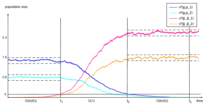
Figure 2. The three steps of one invasion phase.

An example: Figure 2 shows the invasion phase of a single mutant with trait $(\tilde{g},\tilde{p}_{1})$, which appeared (at time $0$) in a population close to $\bar{n}(\mathbf{g},\mathbf{p})$ (indicated by the dashed lines). In this example the resident population consists of two coexisting traits $(g,p_{1})$ and $(g,p_{2})$ and the mutant individuals can switch to one other phenotype only, i.e.  $[\tilde{p}_{1}]_{\tilde{g}}=\{\tilde{p}_{1},\tilde{p}_{2}\}$. The parameters of the simulation of Figure 2 are given in Table 1.

$b(p_{1})=3$	$d({p_{1}})=1$	$c({p_{1}},{p_{1}})=1$	$c({p_{1}},p_{2})=0.7$	$c({p_{1}},\tilde{p}_{1})=0.7$	$c(p_{1},\tilde{p}_{2})=0.7$	$s_{\text{nat.}}^{g}(p_{1},p_{2})=1$
$b(p_{2})=3$	$d({p_{2}})=1$	$c({p_{2}},{p_{1}})=0.7$	$c({p_{2}},p_{2})=1$	$c({p_{2}},\tilde{p}_{1})=0.7$	$c(p_{2},\tilde{p}_{2})=0.7$	$s^{g}_{\text{nat.}}(p_{2},p_{1})=2$
$b(\tilde{p}_{1})=5$	$d(\tilde{p}_{1})=1$	$c(\tilde{p}_{1},{p_{1}})=0.7$	$c(\tilde{p}_{1},p_{2})=0.7$	$c(\tilde{p}_{1},\tilde{p}_{1})=1$	$c(\tilde{p}_{1},\tilde{p}_{2})=0.7$	$s^{\tilde{g}}_{\text{nat.}}(\tilde{p}_{1},\tilde{p}_{2})=1.5$
$b(\tilde{p}_{2})=4$	$d({\tilde{p}_{2}})=1$	$c({\tilde{p}_{2}},{p_{1}})=0.7$	$c({\tilde{p}_{2}},p_{2})=0.7$	$c({\tilde{p}_{2}},\tilde{p}_{1})=0.7$	$c(\tilde{p}_{2},\tilde{p}_{2})=1$	$s^{\tilde{g}}_{\text{nat.}}(\tilde{p}_{2},\tilde{p}_{1})=2$
$K=2000$	$u_{K}=0$	$\nu_{0}^{K}(g,p_{1})=1.5$	$\nu_{0}^{K}(g,p_{2})=0.8$	$\nu_{0}^{K}(\tilde{g},\tilde{p}_{1})=1/K$	$\nu_{0}^{K}(\tilde{g},\tilde{p}_{2})=0$	$s_{\text{ind.}}^{.}(\>.\>,\>.\>)(.)\equiv 0$

Table 1. Parameters of Figure 2

The stable fixed point of the system $LVS(2,((g,p_{1}),(g,p_{2})))$ is $\bar{n}((g,p_{1}),(g,p_{2}))\approx(1.507,0.809)$. The infinitesimal generator of the multi-type branching process that approximates the mutant population in the first step is approximately

$$\left(\begin{matrix}0.879&1.5\\ 2&-0.621\end{matrix}\right).$$ (3.14)

Since the largest eigenvalue of this matrix is positive ($\approx 2.016$), the mutant population reaches with positive probability the second invasion step (cf. Fig.  2).
Moreover, $n^{*}\approx(0,0,2.608,1.608)$ is the unique locally strictly stable fixed point of the dynamical system $LVS(4,((g,p_{1}),(g,p_{2}),(\tilde{g},\tilde{p}_{1}),(\tilde{g},\tilde{p}_{2})))$. The dynamical system and hence also the stochastic process reach in finite time the ${\epsilon}$-neighbourhood of this value. The infinitesimal generator of the multi-type branching process that approximates the resident population in the third step is approximately

$$\left(\begin{matrix}-1.951&2\\ 1&-2.951\end{matrix}\right).$$ (3.15)

The largest eigenvalue of this matrix is negative ($\approx-0.951$) meaning that the process is subcritical and goes extinct a.s.. Therefore, there exists a time $t_{3}$ such that all individuals which carry trait $(g,p_{1})$ or $(g,p_{2})$ are a.s. dead at time $t_{3}$.

3.3. Proof of Theorem 3.3.

In this paragraph we prove the convergence to the PESP. (The proof uses the same arguments and techniques as [10], which were developed in [8]. However, some extensions are necessary, if fast phenotypic switches are included in the process, which we state and prove in this subsection.) We start with an analog of Theorem 3 of [8]. Part (i) of the following theorem strengthens Theorem 2.1, and part (ii) provides control of exit from an attractive domain in the polymorphic case with phenotypic plasticity.

Theorem 3.4.

1. Assume that the initial conditions have support $\{(g_{1},p_{1}),\ldots(g_{d},p_{d})\}$ and are uniformly bounded, i.e. , for all $1\leq i\leq d$, $\nu_{0}^{K}(g_{i},p_{i})\in A$, where $A$ is a compact subset of $\mathbb{R}_{>0}$. Then, for all $T>0$

   $$\lim_{K\uparrow\infty}\>\sup_{t\in[0,T]}\>\Big{|}\Big{|}\nu^{K}_{t}-\sum_{x\in\mathcal{X}_{(\mathbf{g},\mathbf{p})}}\mathfrak{n}_{x}(t,\nu^{K}_{0})\delta_{x}\Big{|}\Big{|}_{TV}=0\quad\text{a.s.,}$$ (3.16)

   where $\mathfrak{n}(t,\nu^{K}_{0})\in\mathbb{R}^{|\mathcal{X}_{(\mathbf{g},\mathbf{p})}|}$ denotes the value of the solution of $LVS(d,(\mathbf{g},\mathbf{p}))$ at time $t$ with initial condition $\mathfrak{n}_{x}(0,\nu^{K}_{0})=\nu^{K}_{0}(x)$ for all $x\in\mathcal{X}_{(\mathbf{g},\mathbf{p})}$. Note that the measure $\sum_{x\in\mathcal{X}_{(\mathbf{g},\mathbf{p})}}\mathfrak{n}_{x}(t,\nu^{K}_{0})\delta_{x}$ depends on $K$, since the initial condition and hence the solution of $LVS(d,(\mathbf{g},\mathbf{p}))$ depends on $K$.

2. Let $(g_{1},p_{1}),\ldots,(g_{d},p_{d})\in\mathcal{X}$ coexist. Assume that, for any $K\geq 1$, $\text{Supp}(\nu_{0}^{K})=\mathcal{X}_{(\mathbf{g},\mathbf{p})}$. Let $\tau_{\text{mut.}}$ be the first mutation time. Define the first exit time from the $\xi$-neighbourhood of $\bar{\mathfrak{n}}_{x}(\mathbf{g},\mathbf{p})$ by

   $$\theta^{K,\xi}_{\text{exit}}\equiv\inf\left\{t\geq 0:\exists x\in\mathcal{X}_{(\mathbf{g},\mathbf{p})}:\left|\nu_{t}^{K}(x)-\bar{\mathfrak{n}}_{x}(\mathbf{g},\mathbf{p})\right|>\xi\right\}.$$ (3.17)

   Then there exist $\epsilon_{0}>0$ and $M>0$ such that, for all $\epsilon<\epsilon_{0}$, there exists $V>0$ such that if the initial state of $\nu^{K}$ lies in the $\epsilon$-neighbourhood of $\bar{\mathfrak{n}}_{x}(\mathbf{g},\mathbf{p})$, the probability that $\theta^{K,M\epsilon}_{\text{exit}}$ is larger than $\mathrm{e}^{KV}\wedge\tau_{\text{mut.}}$ converges to one, i.e.

   $$\quad\lim_{K\uparrow\infty}\>\sup_{\mathbf{n}^{K}\in(\mathbb{N}/K)^{|\mathcal{X}_{(\mathbf{g},\mathbf{p})}|}\cap B_{\epsilon}(\bar{\mathfrak{n}}(\mathbf{g},\mathbf{p}))}\mathbb{P}\left[\theta^{K,M\epsilon}_{\text{exit}}\!<\mathrm{e}^{KV}\wedge\tau_{\text{mut.}}\>\Big{|}\>\nu^{K}_{0}(x)=n^{K}_{x}\text{ for all }x\in\mathcal{X}_{(\mathbf{g},\mathbf{p})}\right]=0,$$ (3.18)

   where $\mathbf{n}^{K}\equiv(n^{K}_{x})_{x\in\mathcal{X}_{(\mathbf{g},\mathbf{p})}}$ and $B_{\epsilon}(\bar{\mathfrak{n}}(\mathbf{g},\mathbf{p}))$ denotes the $\epsilon$-neighbourhood of $\bar{\mathfrak{n}}(\mathbf{g},\mathbf{p})$.

   Moreover, (3.18) also holds if, for all $(g,p)\in\mathcal{X}_{(\mathbf{g},\mathbf{p})}$, the total death rate of an individual with trait $(g,p)$,

   $$d(p)+\sum_{(\tilde{g},\tilde{p})\in\mathcal{X}_{(\mathbf{g},\mathbf{p})}}c(p,\tilde{p})\nu^{K}_{t}(\tilde{g},\tilde{p}),$$ (3.19)

   and the total switch rates of an individual with trait $(g,p)$,

   $$s^{g}_{\text{nat.}}(p,p_{i})+\sum_{(\tilde{g},\tilde{p})\in\mathcal{X}_{(\mathbf{g},\mathbf{p})}}s^{g}_{\text{ind.}}(p,p_{i})(\tilde{p})\nu^{K}_{t}(\tilde{g},\tilde{p})\quad\text{for all }p_{i}\in[p]_{g},$$ (3.20)

   are perturbed by additional random processes that are uniformly bounded by $\bar{c}\epsilon$ respectively $\bar{s}_{\text{i}nd.}\epsilon$, where $\bar{c}$ and $\bar{s}_{\text{i}nd.}$ are upper bounds for the parameters of competition and induced switch.

Remark 6.

1. One consequence of the second part of (ii) is that, with high probability, the process stays in the $M\epsilon$-neighbourhood of $\bar{\mathfrak{n}}_{x}(\mathbf{g},\mathbf{p})$ until the first time that a mutant’s density reaches the value $\epsilon$. In other words, let $\theta^{K}_{\text{Invasion}}$ denote the first time that a mutant’s density reaches the value $\epsilon$, i.e

   $$\theta^{K}_{\text{Invasion}}\equiv\left\{\>t\geq 0:\exists(g,p)\notin\mathcal{X}_{(\mathbf{g},\mathbf{p})}:\textstyle\sum_{\tilde{p}\in[p]_{g}}\nu^{K}_{t}(g,\tilde{p})\geq\epsilon\>\right\}.$$ (3.21)

   Then, the probability that $\theta^{K,M\epsilon}_{\text{exit}}$ is larger than $\mathrm{e}^{KV}\wedge\theta^{K}_{\text{Invasion}}$ converges to one. We use this result also for the third invasion step.

2. Since $\bar{\mathfrak{n}}(\mathbf{g},\mathbf{p})$ is a locally strictly stable fixed point of the system $LVS(d,(\mathbf{g},\mathbf{p}))$, there exists a constant $M>0$ such that, for all $\epsilon>0$ small enough, for all trajectories $\mathfrak{n}(t)$ with $||\mathfrak{n}(0)-\bar{\mathfrak{n}}(\mathbf{g},\mathbf{p})||<\epsilon$, it holds that $\sup_{t\geq 0}||\mathfrak{n}(t)-\bar{\mathfrak{n}}(\mathbf{g},\mathbf{p})||<M\epsilon$.

Proof.

The main task to prove (i) is to show that a large deviation principle on $[0,T]$ holds for a sightly modify process and that the $\nu^{K}$ has the same law on the random time interval we need to control it. In fact, Theorem 10.2.6 of [13] can be applied to obtain the large deviation principle. The main task to prove (ii) is to show that the classical estimates for exit times from a domain (cf. [16]) for the jump process $\nu^{K}$ can be used. Note that Freidlin and Wentzell study in [16] mainly small white noise perturbations of dynamical systems. However, there also are some comments on the generalisation to dynamical systems with small jump-like perturbations (cf. [16], Sec. 5.4). ∎

The following Lemma describes the asymptotic behaviour of $\tau_{\text{mut.}}$ and can be seen as an extension of Lemma 2 of [8] or Lemma A.3 of [10].

Lemma 3.5.

Let $(g_{1},p_{1}),...,(g_{d},p_{d})\in\mathcal{X}$ coexist. Assume that, for any $K\geq 1$, $\text{Supp}(\nu_{0}^{K})=\mathcal{X}_{(\mathbf{g},\mathbf{p})}$. Let $\tau_{\text{mut.}}$ denote the first mutation time. Then, there exists $\epsilon_{0}>0$ such that if the initial states of $\nu^{K}$ belong to the $\epsilon_{0}$-neighbourhood of $\bar{\mathfrak{n}}_{x}(\mathbf{g},\mathbf{p})$, then, for all $\epsilon\in(0,\epsilon_{0})$,

$$\lim_{K\uparrow\infty}\>\mathbb{P}\left[\tau_{\text{mut.}}>\ln(K),\sup_{t\in[\ln(K),\tau_{\text{mut.}}]}\>\>\Big{|}\Big{|}\nu^{K}_{t}-\textstyle\sum_{x\in\mathcal{X}_{(\mathbf{g},\mathbf{p})}}\bar{\mathfrak{n}}_{x}(\mathbf{g},\mathbf{p})\delta_{x}\Big{|}\Big{|}_{TV}<\epsilon\right]=1,$$ (3.22)

Moreover, $(\tau_{\text{mut.}}u_{K}K)_{K\geq 1}$ converges in law to an exponential distributed random variable with parameter $\sum_{(g,p)\in\mathcal{X}_{(\mathbf{g},\mathbf{p})}}m(g)b(p)\bar{\mathfrak{n}}_{(g,p)}(\mathbf{g},\mathbf{p})$ and the probability that the mutant, which appears at time $\tau_{\text{mut.}}$, is born from an individual with trait $(g,p)\in\mathcal{X}_{(\mathbf{g},\mathbf{p})}$ converges to

$$\frac{m(g)b(p)\bar{\mathfrak{n}}_{(g,p)}(\mathbf{g},\mathbf{p})}{\sum_{(\tilde{g},\tilde{p})\in\mathcal{X}_{(\mathbf{g},\mathbf{p})}}m(\tilde{g})b(\tilde{p})\bar{\mathfrak{n}}_{(\tilde{g},\tilde{p})}(\mathbf{g},\mathbf{p})}$$ (3.23)

as $K\uparrow\infty$.

Proof.

There exist constants $C>0$ and $V>0$, such that on the time interval $[0,\exp(KV)]$ the total mass of the population, $\nu_{t}^{K}(\mathcal{X})$, is bounded from above by $C$. Therefore, we can construct an exponential random variable $A$ with parameter $C^{\prime}Ku_{K}$, where $C^{\prime}=C\max_{g\in\mathcal{G},p\in\mathcal{P}}m(g)b(p)$, such that

$$A\leq\tau_{\text{mut.}}\qquad\text{ on the event }\quad\left\{\tau_{\text{mut.}}<\exp(KV)\right\}.$$ (3.24)

Thus, $\mathbb{P}\left[\tau_{\text{mut.}}>\ln(K)\right]\geq\mathbb{P}\left[A>\ln(K)\right]=\mathrm{e}^{-C^{\prime}\ln(K)Ku_{K}}$. Since $(\ref{Conv_Cond})$ implies that $\ln(K)Ku_{K}$ converges to zero as $K\uparrow\infty$, we get $\lim_{K\uparrow\infty}\mathbb{P}[\tau_{\text{mut.}}>\ln(K)]=1$.

The fixed point $\bar{\mathfrak{n}}(\mathbf{g},\mathbf{p})$ is asymptotic stable. Thus, $\exists\epsilon_{0}>0:\forall\tilde{\epsilon}\in(0,\epsilon_{0})\>\exists T(\tilde{\epsilon})$:

$$\|\mathfrak{n}(\mathbf{g},\mathbf{p})(0)-\bar{\mathfrak{n}}(\mathbf{g},\mathbf{p})\|<\epsilon_{0},\qquad\text{ implies }\quad\sup_{t\geq T(\tilde{\epsilon})}|\mathfrak{n}(\mathbf{g},\mathbf{p})(t)-\bar{\mathfrak{n}}(\mathbf{g},\mathbf{p})|<\tilde{\epsilon}/2.$$ (3.25)

In words, there exists a finite time $T(\tilde{\epsilon})$ such that all trajectories, which start in the $\epsilon_{0}$ neighbourhood of the fixed point, stay after $T(\tilde{\epsilon})$ in the $\tilde{\epsilon}/2$-neighbourhood of the fixed point.

Next, we apply the last theorem: By (i), for all $\tilde{\epsilon}\in(0,\epsilon_{0})\>\exists T(\tilde{\epsilon})$ such that, for $K$ large enough,

$$\Big{|}\Big{|}\nu^{K}_{T(\tilde{\epsilon})}-\textstyle\sum_{x\in\mathcal{X}_{(\mathbf{g},\mathbf{p})}}\bar{\mathfrak{n}}_{x}(\mathbf{g},\mathbf{p})\delta_{x}\Big{|}\Big{|}_{TV}<\tilde{\epsilon}\quad a.s..$$ (3.26)

Then, by (ii), there exist ${\epsilon}_{0}>0$ and $M>0$: for all $\tilde{\epsilon}\in(0,\epsilon_{0})$ there exists $V>0$ such that

$$\lim_{K\uparrow\infty}\mathbb{P}\left[\sup_{t\in[T(\tilde{\epsilon}),\>\mathrm{e}^{KV}\!\wedge\tau_{\text{mut.}})}\>\Big{|}\Big{|}\nu^{K}_{t}-\textstyle\sum_{x\in\mathcal{X}_{(\mathbf{g},\mathbf{p})}}\bar{\mathfrak{n}}_{x}(\mathbf{g},\mathbf{p})\delta_{x}\Big{|}\Big{|}_{TV}<M\tilde{\epsilon}\right]=1.$$ (3.27)

Moreover, for all $\tilde{\epsilon}\in(0,\epsilon_{0})$ there exists $K_{0}\in\mathbb{N}$ such that $T(\tilde{\epsilon})<\ln(K)$ for all $K\geq K_{0}$. Thus, setting $\epsilon=M\tilde{\epsilon}$, ends the proof of (3.22), provided that $\lim_{K\uparrow\infty}{\mathbb{P}}[\tau_{\text{mut.}}<\mathrm{e}^{KV}]=1$.

Again, we can construct for all $\epsilon>0$ two exponential random variables $A^{1,K,\epsilon}$ and $A^{2,K,\epsilon}$ with parameters

$$a_{1}u_{K}K\equiv\sum_{(g,p)\in\mathcal{X}_{(\mathbf{g},\mathbf{p})}}u_{K}m(g)b(p)(\bar{\mathfrak{n}}_{(g,p)}(\mathbf{g},\mathbf{p})+\epsilon)K$$ (3.28)

and

$$a_{2}u_{K}K\equiv\sum_{(g,p)\in\mathcal{X}_{(\mathbf{g},\mathbf{p})}}u_{K}m(g)b(p)(\bar{\mathfrak{n}}_{(g,p)}(\mathbf{g},\mathbf{p})-\epsilon)K$$ (3.29)

such that

$$A^{1,K,\epsilon}\leq\tau_{\text{mut.}}\leq A^{2,K,\epsilon}\quad\qquad\text{on the event }\{T(\tilde{\epsilon})<\tau_{\text{mut.}}<\mathrm{e}^{KV}\},$$ (3.30)

where $T(\tilde{\epsilon})$ is the time defined in equation (3.26) and $\tilde{\epsilon}={\epsilon}/M$. Moreover, we have

$$\lim_{K\uparrow\infty}\mathbb{P}[\tau_{\text{mut.}}<\ln(K)]=0\qquad\text{and}\qquad\lim_{K\uparrow\infty}\mathbb{P}[A^{2,K,\epsilon}>\mathrm{e}^{KV}]=0,$$ (3.31)

because $u_{K}K\mathrm{e}^{KV}\uparrow\infty$ as $K\uparrow\infty$. Therefore, for all $\epsilon>0$, the probability of the event $\{T(\tilde{\epsilon})<\tau_{\text{mut.}}<\mathrm{e}^{KV}\}$ converges to one as $K$ goes to infinity. Moreover, the random variables $A^{1,K,\epsilon}u_{K}K$ and $A^{2,K,\epsilon}u_{K}K$ converge both in law to the same exponential distributed random variable with parameter

$$\sum_{(g,p)\in\mathcal{X}_{(\mathbf{g},\mathbf{p})}}m(g)b(p)\bar{\mathfrak{n}}_{(g,p)}(\mathbf{g},\mathbf{p})$$ (3.32)

as first $K\uparrow\infty$ and then $\epsilon\to 0$. The random variables $A$, $A^{1,K,\epsilon}$ and $A^{2,K,\epsilon}$ can easily be constructed by using the pathwise description of $\nu^{K}$ (cf. [3] or [9]). ∎

Theorem 3.6 (The three steps of invasion).

Let $(g_{1},p_{1}),\ldots,(g_{d},p_{d})\in\mathcal{X}$ coexist. Assume that, for any $K\geq 1$, $\text{Supp}(\nu_{0}^{K})=\mathcal{X}_{(\mathbf{g},\mathbf{p})}\cup\{(\tilde{g},\tilde{p})\}$. Let $\tau_{\text{mut.}}$ denote the next mutation time (after time zero) and define

$$\theta^{K,\xi}_{\text{No Jump}} \equiv \inf\Big{\{}t\geq 0:\nu^{K}_{t}(\tilde{g})=0\;\text{ and }\;\Big{|}\Big{|}\nu_{t}^{K}-\textstyle\sum_{x\in\mathcal{X}_{(\mathbf{g},\mathbf{p})}}\bar{\mathfrak{n}}_{x}(\mathbf{g},\mathbf{p})\delta_{x}\Big{|}\Big{|}_{TV}<\xi\Big{\}}$$ (3.33)

$$\theta^{K,\xi}_{\text{Jump}} \equiv \inf\Big{\{}t\geq 0:\Big{|}\Big{|}\nu_{t}^{K}-\textstyle\sum_{x\in\mathcal{X}_{((\mathbf{g},\mathbf{p}),(\tilde{g},\tilde{p}))}}\mathfrak{n}^{*}_{x}((\mathbf{g},\mathbf{p}),(\tilde{g},\tilde{p}))\delta_{x}\Big{|}\Big{|}_{TV}<\xi$$

$$\hskip 56.9055pt\text{ and }\;\forall\hat{x}\notin\{x\in\mathcal{X}:\mathfrak{n}^{*}_{x}((\mathbf{g},\mathbf{p}),(\tilde{g},\tilde{p}))>0\}:\>\nu^{K}_{t}(\hat{x})=0\Big{\}}.$$

Assume that we have a single initial mutant, i.e. $\nu^{K}_{0}(\tilde{g},\tilde{p})=1/K$. Then, there exist $\epsilon_{0}>0,C>0,$ and $M>0$ such that for all $\epsilon\in(0,\epsilon_{0})$ if $||\nu_{0}^{K}-\textstyle\sum_{x\in\mathcal{X}_{(\mathbf{g},\mathbf{p})}}\bar{\mathfrak{n}}_{x}(\mathbf{g},\mathbf{p})\delta_{x}||_{TV}<\epsilon$,

$$\lim_{K\uparrow\infty}\mathbb{P}\left[\theta^{K,M\epsilon}_{\text{No Jump}}<\theta^{K,M\epsilon}_{\text{Jump}}\right] \geq q_{{(\mathbf{g},\mathbf{p})}}(\tilde{g},\tilde{p})-C{\epsilon},$$ (3.35)

$$\lim_{K\uparrow\infty}\mathbb{P}\left[\theta^{K,M\epsilon}_{\text{Jump}}<\theta^{K,M\epsilon}_{\text{No Jump}}\right] \geq 1-q_{{(\mathbf{g},\mathbf{p})}}(\tilde{g},\tilde{p})-C{\epsilon},$$ (3.36)

where $1-q_{{(\mathbf{g},\mathbf{p})}}(\tilde{g},\tilde{p})$ is the invasion probability defined in (3.8) and

$$\forall\eta>0,\quad\lim_{K\uparrow\infty}\mathbb{P}\left[\theta^{K,M\epsilon}_{\text{Jump}}\wedge\theta^{K,M\epsilon}_{\text{No Jump}}\geq\frac{\eta}{u_{K}K}\wedge\tau_{\text{mut.}}\right]\leq C{\epsilon}.$$ (3.37)

The structure of the proof is similar to the one of Lemma 3 in [8] (cf. also Lem.  A.4. of [10]). However, we have to extend the theory to multi-type branching processes. Thus, the proof is not a simple copy the arguments in [8]. Before proving the theorem, let us collect some properties about multi-type continuous-time branching processes. Most of these can be found in [2] or [23]. The limit theorems we need in the sequel were first obtained by Kesten and Stigum [19, 18, 20] in the discrete-time case and by Athreya [1] in the continuous-time case.

Let $Z(t)$ be a $k$-dimensional continuous-time branching process. Assume that $Z(t)$ is non-singular and that the first moments exist. (Note that a process is singular if and only if each individual has exactly one offspring and that the existence of the first moments is sufficient for the non-exposition hypothesis.) Then, the so-called mean matrix $M(t)$ of $Z(t)$ is the $k\times k$ matrix with elements

$$m_{ij}(t)\equiv\mathbb{E}[Z_{j}(t)|Z(0)=\mathbf{e}_{i}],\quad 1\leq i,j\leq k,$$ (3.38)

and $\mathbf{e}_{i}$ is the $i$-th unit vector in $\mathbb{R}^{k}$. It is well known (cf.  [2] p. 202) that there exists a matrix $\mathbf{A}$, called the infinitesimal generator of the semigroup $\{\mathbf{M}(t),t\geq 0\}$, such that

$$\mathbf{M}(t)\equiv\exp(\mathbf{A}t)=\sum_{n=0}^{\infty}\frac{t^{n}(\mathbf{A})^{n}}{n!}.$$ (3.39)

Furthermore, let $\mathbf{r}=(r_{1},\ldots,r_{k})$ be the vector of the branching rates, meaning that every individual of type $i$ has an exponentially distributed lifetime of parameter $r_{i}$ and let $\mathbf{M}$ be the mean matrix of the corresponding discrete-time process, i.e. $\mathbf{M}\equiv\{m_{ij},\;i,j=1,\ldots,k\}$, where $m_{ij}$ is the expected number of type $j$ offspring of a single type-$i$-particle in one generation. Then, we can identify the infinitesimal generator $\mathbf{A}$ as

$$\mathbf{A}=\mathbf{R}(\mathbf{M}-\mathbf{I}),$$ (3.40)

where $\mathbf{R}=diag(r_{1},\ldots,r_{k})$, i.e. $r_{ij}=r_{i}\delta_{i}(j)$ and $\mathbf{I}$ is the identity matrix of size $k$.

Under the basic assumption of positive regularity, i.e. that there exists a time $t_{0}$ such that $\mathbf{M}(t_{0})$ has strictly positive entries, the Perron-Frobenius theory asserts that

1. the largest eigenvalue of $\mathbf{M}(t_{0})$ is real-valued and strictly positive,

2. the algebraic and geometric multiplicities of this eigenvalue are both one, and

3. the corresponding eigenvector has strictly positive cmponents.

By (3.39), the eigenvalues of $\mathbf{M}(t)$ are given by $\exp({\lambda_{i}t})$, where $\{{\lambda}_{i};i=1,\ldots,k\}$ are the eigenvalues of $\mathbf{A}$, and both matrices have the same eigenvectors, which implies that the left and right eigenvectors $\mathbf{u}$ and $\mathbf{v}$ of ${\lambda}_{\text{max}}(\mathbf{A})$ can be chosen with strictly positive components and satisfying

$$\textstyle\sum_{i=1}^{k}v_{i}u_{i}=1\quad\text{and}\quad\sum_{i=1}^{k}u_{i}=1.$$ (3.41)

The process $Z$ is called supercritical, critical, or subcritical according as ${\lambda}_{\text{max}}(\mathbf{A})$ is larger, equal, or smaller than zero.

Observe that the following properties are equivalent (cf.  [23] p. 95-99 and [22]):
$Z$ is irreducible   $\Leftrightarrow$  $\mathbf{M}$ is irreducible   $\Leftrightarrow$  $\mathbf{A}$ is irreducible   $\Leftrightarrow$  $\mathbf{M}(t)$ is irreducible for all $t>0$   $\Leftrightarrow$  $\mathbf{M}(t)>0$ for all $t>0$.
In particular, irreducible implies positive regular. Note that a matrix is irreducible if it is not similar via a permutation to a block upper triangular matrix and that a Markov chain is irreducible if and only if the mean matrix is irreducible.

The following lemma is an extension of Theorem 4 of [8] for multi-type branching processes.

Lemma 3.7.

Let $(Z(t))_{t\geq 0}$ be a non-singular and irreducible $k$-dimensional continuous-time Markov branching process and $\mathbf{q}$ the extinction vector of $Z$, i.e.

$$q_{i}\equiv\mathbb{P}[Z(t)=0\text{ for some }t\geq 0|Z(0)=\mathbf{e}_{i}]\quad\text{ for $1\leq i\leq k$}.$$ (3.42)

Furthermore, let $(t_{K})_{K\geq 1}$ be a sequence of positive numbers such that $\ln(K)\ll t_{K}$, define $T_{\rho}\equiv\inf\{t\geq 0:\sum_{i=1}^{k}Z_{i}(t)=\rho\}$ and assume that, for all $i,j\in\{1,\ldots,k\}$ and $t\in[0,\infty)$,

$$\mathbb{E}[Z_{j}(t)\ln(Z_{j}(t))|Z(0)=\mathbf{e}_{i}]<\infty.$$ (3.43)

1. If $Z$ is subcritical, i.e. ${\lambda}_{\text{max}}(\mathbf{A})<0$, then for any $\epsilon>0$

   $$\lim_{K\uparrow\infty}\mathbb{P}\left[T_{0}\leq t_{K}\wedge T_{\lceil{\epsilon}K\rceil}\>\middle|\>Z(0)=\mathbf{e}_{i}\right]=1\qquad\text{ for all }i\in\{1,\ldots,k\}$$ (3.44)

   and

   $$\lim_{K\uparrow\infty}\,\inf_{\mathbf{x}\in\partial B_{{\epsilon}K}}\mathbb{P}\left[T_{0}\leq t_{K}\,\middle|\,Z(0)=\mathbf{x}\right]=1,\quad\text{ where }\partial B_{{\epsilon}K}\equiv\{\mathbf{x}\in\mathbb{N}_{0}^{k}:\textstyle\sum_{i=1}^{k}x_{i}=\lceil{\epsilon}K\rceil\}.$$ (3.45)

   Moreover, for $\bar{u}=\frac{\max_{1\leq i\leq k}u_{i}}{\min_{1\leq j\leq k}u_{j}}$ and for any ${\epsilon}>0$,

   $$\quad\lim_{K\uparrow\infty}\sup_{\mathbf{x}\in B_{{\epsilon}^{2}K}}\mathbb{P}\left[T_{\lceil{\epsilon}K\rceil}\leq T_{0}\>\middle|\>Z(0)=\mathbf{x}\right]\leq\bar{u}{\epsilon},\quad\text{where }B_{{\epsilon}^{2}K}\equiv\{\mathbf{x}\in\mathbb{N}_{0}^{k}:\textstyle\sum_{i=1}^{k}x_{i}\leq\lceil{\epsilon}^{2}K\rceil\}.$$ (3.46)

2. If $Z$ is supercritical, i.e. ${\lambda}_{\text{max}}(\mathbf{A})>0$, then for any $\epsilon>0$ (small enough)

   $$\lim_{K\uparrow\infty}\mathbb{P}\left[T_{0}\leq t_{K}\wedge T_{\lceil{\epsilon}K\rceil}\>\middle|\>Z(0)=\mathbf{e}_{i}\right]=q_{i}\qquad\text{ for all }i\in\{1,\ldots,k\}$$ (3.47)

   and

   $$\lim_{K\uparrow\infty}\mathbb{P}\left[T_{\lceil{\epsilon}K\rceil}\leq t_{K}\>\middle|\>Z(0)=\mathbf{e}_{i}\right]=1-q_{i}\qquad\text{ for all }i\in\{1,\ldots,k\}.$$ (3.48)

   Moreover, conditionally on survival, the proportions of the different types present in the population converge almost surely, as $t\uparrow\infty$, to the corresponding ratios of the components of the eigenvector: for all $i=1,\ldots,k,$

   $$\lim_{t\uparrow\infty}\frac{Z_{i}(t)}{\sum_{j=1}^{k}Z_{j}(t)}=\frac{v_{i}}{\sum_{j=1}^{k}v_{j}},\quad\text{a.s. on }\{T_{0}=\infty\}.$$ (3.49)

Proof.

We start with the proof of (i). Since $Z(t)$ is in this case a subcritical irreducible continuous-time branching process and $\mathbb{E}[Z_{j}(t)\ln(Z_{j}(t))|Z(0)=\mathbf{e}_{i}]<\infty$, we obtain by applying Satz 6.2.7 of [23] the existence of a constant $C>0$ such that

$$\lim_{t\uparrow\infty}\frac{1-q_{i}(t)}{\mathrm{e}^{{\lambda}_{\text{max}}(\mathbf{A})t}}=Cu_{i},$$ (3.50)

where $q_{i}(t)\equiv\mathbb{P}[Z(t)=0\>|\>Z(0)=\mathbf{e}_{i}]$. Moreover, we have a non-explosion condition. Thus, for all $\epsilon>0$, either $T_{\lceil{\epsilon}K\rceil}$ equals infinity or it converges to infinity as $K\uparrow\infty$. Putting both together, there exists a sequence $s_{K}$ with $\lim_{K\uparrow\infty}s_{K}=+\infty$ such that

$$\lim_{K\uparrow\infty}\mathbb{P}\left[T_{0}\leq t_{K}\wedge T_{\lceil{\epsilon}K\rceil}\middle|Z(0)=\mathbf{e}_{i}\right]\geq\lim_{K\uparrow\infty}\mathbb{P}\left[T_{0}\leq s_{K}\>\middle|\>Z(0)=\mathbf{e}_{i}\right]=\lim_{K\uparrow\infty}q_{i}(s_{K})=1.$$ (3.51)

The branching property implies that for all $\mathbf{x}\in\mathbb{N}^{k}$, $\mathbb{P}[Z(t)=0\>|\>Z(0)=\mathbf{x}]=\prod_{i=1}^{k}(q_{i}(t))^{x_{i}}$ (cf. [22] p. 25). So, we get

$$\inf_{\mathbf{x}\in\partial B_{{\epsilon}K}}\!\mathbb{P}\left[T_{0}\leq t_{K}\>\middle|\>Z(0)=\mathbf{x}\right]=\inf_{\mathbf{x}\in\partial B_{{\epsilon}K}}\!\mathbb{P}\left[Z(t_{K})=0\>\middle|\>Z(0)=\mathbf{x}\right]=\inf_{\mathbf{x}\in\partial B_{{\epsilon}K}}\prod_{i=1}^{k}(q_{i}(t_{K}))^{x_{i}}.$$ (3.52)

For all $i\in\{1,\ldots,k\}$, $1\geq(q_{i}(t_{K}))^{x_{i}}\geq(q_{i}(t_{K}))^{\lceil{\epsilon}K\rceil}$ and by (3.50) we have $1-q_{i}(t_{K})=O(\mathrm{e}^{{{\lambda}_{\text{max}}(\mathbf{A})t_{K}}})$. Moreover, for any sequence $(w_{K})_{K\geq 1}$ such that $\lim_{K\uparrow\infty}w_{K}=0$,

$$\lim_{K\uparrow\infty}\left(1+\frac{w_{K}}{K}\right)^{K}=1.$$ (3.53)

This implies that, for all $t_{K}$ with $t_{K}\gg\ln(K)$ and $C>0$, since $\lim_{K\uparrow\infty}C\mathrm{e}^{{\lambda}_{\text{max}}(\mathbf{A})t_{k}}\lceil{\epsilon}K\rceil=0$,

$$\lim_{K\uparrow\infty}(1-C\mathrm{e}^{{\lambda}_{\text{max}}(\mathbf{A})t_{k}})^{\lceil{\epsilon}K\rceil}=1.$$ (3.54)

Thus, taking the limit $K\uparrow\infty$ in (3.52), we obtain the desired equation (3.45). To prove the inequality (3.46) we use the fact that $(\sum_{i=1}^{k}u_{i}Z_{i}(t))\mathrm{e}^{-\lambda_{\text{max}}t}$ is a martingale (cf. [1], Prop.  2). By applying Doob’s stopping theorem to the stopping time $T_{\lceil{\epsilon}K\rceil}\wedge T_{0}$ we obtain, for all $\mathbf{x}\in B_{{\epsilon}^{2}K}$, that

$$\textstyle\mathbb{E}\left[\left(\sum_{i=1}^{k}u_{i}Z_{i}(T_{\lceil{\epsilon}K\rceil})\right)\mathrm{e}^{-\lambda_{\text{max}}(\mathbf{A})T_{\lceil{\epsilon}K\rceil}}\mathds{1}_{\{T_{\lceil{\epsilon}K\rceil}<T_{0}\}}\middle|Z(0)=\mathbf{x}\right]=\sum_{i=1}^{k}u_{i}x_{i}.$$ (3.55)

Therefore, since $\lambda_{\text{max}}(\mathbf{A})<0$ in the subcritical case,

$$\mathbb{E}\left[\min_{1\leq i\leq k}u_{i}\lceil{\epsilon}K\rceil\mathds{1}_{\{T_{\lceil{\epsilon}K\rceil}<T_{0}\}}\middle|Z(0)=\mathbf{x}\right]\leq\max_{1\leq i\leq k}u_{i}\lceil{\epsilon}^{2}K\rceil,\quad\text{ for all $\mathbf{x}\in B_{{\epsilon}^{2}K}$},$$ (3.56)

which implies (3.46).

Let us continue by proving (ii). Since $Z(t)$ is supercritical in this case, applying Theorem 5.7.2 of [2] yields that

$$\lim_{t\uparrow\infty}Z(t)({\omega})\mathrm{e}^{-{\lambda}_{\text{max}}(\mathbf{A})t}=W(\omega)\mathbf{v},\hbox{\rm a.s.},$$ (3.57)

where $W$ is a nonnegative random variable. Since we assume that, for all $i\in\{1,\ldots,k\}$,
$\mathbb{E}[Z_{j}(t)\ln(Z_{j}(t))|Z(0)=\mathbf{e}_{i}]<\infty$, we get that

$$\mathbb{P}[W=0|Z(0)=\mathbf{e}_{i}]=q_{i},\quad\mathbb{E}[W|Z(0)=\mathbf{e}_{i}]=u_{i},$$ (3.58)

and $W$ has an absolutely continuous distribution on $(0,\infty)$. All components of $\mathbf{v}$ are strictly positive and $W>0$, a.s., on the event $\{{\omega}:T_{0}({\omega})=\infty\}$. Hence, we have

$$Z(t)=O\left(\mathrm{e}^{{\lambda}_{\text{max}}(\mathbf{A})t}\right)\quad\text{ a.s.\quad on }\{T_{0}=\infty\}.$$ (3.59)

This implies, for $K$ large enough, $\mathbb{P}[Z(t_{K})<\lceil{\epsilon}K\rceil,T_{0}=\infty]=0$ and thus

$$\lim_{K\uparrow\infty}\mathbb{P}[T_{0}=\infty,\>T_{\lceil{\epsilon}K\rceil}\geq t_{K}]=0.$$ (3.60)

Note that we used that $t_{K}\gg\ln(K)$. Since $\mathbb{P}\left[T_{0}=\infty|Z(0)=\mathbf{e}_{i}\right]=1-q_{i}$, we deduce (3.48). On the other hand, there exist two sequences $s^{1}_{K}$ and $s^{2}_{K}$, which converge to infinity as $K\uparrow\infty$, such that, for $K$ large enough, $s_{K}^{1}\leq t_{K}\wedge T_{\lceil{\epsilon}K\rceil}\leq s_{K}^{2}$ a.s.. This implies (3.47), because for all $i\in\{1,\ldots k\}$ and $l=1,2$, hold $\lim_{K\uparrow\infty}\mathbb{P}[T_{0}<s_{K}^{l}|Z_{0}=\mathbf{e}_{i}]=q_{i}$. Note that equation (3.49) is a simple consequence of (3.57). ∎

Using these properties about multi-type branching processes we can now prove the theorem about the three steps of invasion.

Proof of Theorem 3.6.

The first invasion step. Let us introduce the following stopping times

$$\theta^{K,M\epsilon}_{\text{exit}} = \inf\Big{\{}t\geq 0:||\nu_{t}^{K}-\textstyle\sum_{x\in\mathcal{X}_{(\mathbf{g},\mathbf{p})}}\bar{\mathfrak{n}}_{x}(\mathbf{g},\mathbf{p})\delta_{x}||_{TV}>M\epsilon\Big{\}}$$ (3.61)

$$\tilde{\theta}^{K}_{\epsilon} = \inf\Big{\{}t\geq 0:\>\nu_{t}^{K}(\tilde{g})\geq\epsilon\>\Big{\}}$$ (3.62)

$$\tilde{\theta}^{K}_{0} = \inf\Big{\{}t\geq 0:\>\nu_{t}^{K}(\tilde{g})=0\>\Big{\}}$$ (3.63)

Until $\tilde{\theta}^{K}_{\epsilon}$ the mutant population $\nu_{t}^{K}(\tilde{g})$ influences only the death and switching rates of the resident population and this perturbation is uniformly bounded by $(\bar{c}+\bar{s}_{\text{ind.}})\epsilon$. Thus, by applying Theorem 3.4 (ii), we obtain

$$\lim_{K\uparrow\infty}\mathbb{P}\left[\theta^{K,M\epsilon}_{\text{exit}}<\mathrm{e}^{KV}\!\wedge\tau_{\text{mut.}}\wedge\tilde{\theta}^{K}_{\epsilon}\right]=0.$$ (3.64)

On the time interval $[0,\theta^{K,M\epsilon}_{\text{exit}}\wedge\tau_{\text{mut.}}\wedge\tilde{\theta}^{K}_{\epsilon}]$, the resident population can be approximated by $\textstyle\sum_{x\in\mathcal{X}_{(\mathbf{g},\mathbf{p})}}\bar{\mathfrak{n}}_{x}(\mathbf{g},\mathbf{p})\delta_{x}$ and no further mutant appears. This allows us to approximate $\nu_{t}^{K}(\tilde{g})$ by multi-type branching processes.

Let $k\equiv|[\tilde{p}]_{\tilde{g}}|$. We construct two $(\mathbb{N}_{0})^{k}$- valued processes $X^{1,{\epsilon}}(t)$ and $X^{2,{\epsilon}}(t)$, using the pathwise definition in terms of Poisson point measures of $\nu^{K}_{t}$, which control the mutant population $\nu_{t}^{K}(\tilde{g})$. To this aim let us denote the elements of $[\tilde{p}]_{\tilde{g}}$ by $\tilde{p}_{1},\ldots,\tilde{p}_{k}$ (w.l.o.g. $\tilde{p}\equiv\tilde{p}_{1}$). Then, we define $X^{1,{\epsilon}}$ by

$$X^{1,{\epsilon}}(t) \equiv X^{1,{\epsilon}}(0)+\sum_{j=1}^{k}\int_{0}^{t}\!\int_{\mathbb{N}_{0}}\!\int_{\mathbb{R}_{+}}\mathds{1}_{\left\{i\leq X^{1,{\epsilon}}_{j}({s-}),\;\theta\leq b(\tilde{p}_{i})-\epsilon\right\}}\mathbf{e}_{j}N^{\text{birth}}_{(\tilde{g},\tilde{p}_{j})}(ds,di,d{\theta})$$ (3.65)

$$\quad-\sum_{j=1}^{k}\int_{0}^{t}\!\int_{\mathbb{N}_{0}}\!\int_{\mathbb{R}_{+}}\mathds{1}_{\left\{i\leq X^{1,{\epsilon}}_{j}({s-}),\;\theta\leq d(\tilde{p}_{j})+\sum_{(g,p)\in\mathcal{X}_{(\mathbf{g},\mathbf{p})}}c(\tilde{p}_{j},p)\bar{\mathfrak{n}}_{(g,p)}(\mathbf{g},\mathbf{p})+\bar{c}M\epsilon\right\}}\mathbf{e}_{j}N_{(\tilde{g},\tilde{p}_{j})}^{\text{death}}(ds,di,d{\theta})$$

$$\quad+\sum_{j=1}^{k}\int_{0}^{t}\!\int_{\mathbb{N}_{0}}\!\int_{\mathbb{R}_{+}}\!\int_{[\tilde{p}]_{\tilde{g}}}\mathds{1}_{\left\{i\leq X^{1,{\epsilon}}_{j}({s-}),\>i\neq j\right\}}\>\bigg{(}\>\mathds{1}_{\left\{\theta\leq s_{\text{nat.}}^{\tilde{g}}(\tilde{p}_{j},\tilde{p}_{l})+\sum_{(g,p)\in\mathcal{X}_{(\mathbf{g},\mathbf{p})}}s_{\text{ind.}}^{\tilde{g}}(\tilde{p}_{j},\tilde{p}_{l})(p)\bar{\mathfrak{n}}_{(g,p)}(\mathbf{g},\mathbf{p})-\bar{s}_{\text{ind.}}M\epsilon\right\}}\mathbf{e}_{l}$$

$$\qquad\qquad\qquad-\mathds{1}_{\left\{\theta\leq s_{\text{nat.}}^{\tilde{g}}(\tilde{p}_{j},\tilde{p}_{l})+\sum_{(g,p)\in\mathcal{X}_{(\mathbf{g},\mathbf{p})}}s_{\text{ind.}}^{\tilde{g}}(\tilde{p}_{j},\tilde{p}_{l})(p)\bar{\mathfrak{n}}_{(g,p)}(\mathbf{g},\mathbf{p})+\bar{s}_{\text{ind.}}M\epsilon\right\}}\mathbf{e}_{j}\>\bigg{)}\>N_{(\tilde{g},\tilde{p}_{j})}^{\text{switch}}(ds,di,d{\theta},d\tilde{p}_{l}),$$

and similar $X^{2,{\epsilon}}$ by

$$X^{2,{\epsilon}}(t) \equiv X^{2,{\epsilon}}(0)+\sum_{j=1}^{k}\int_{0}^{t}\!\int_{\mathbb{N}_{0}}\!\int_{\mathbb{R}_{+}}\mathds{1}_{\left\{i\leq X^{2,{\epsilon}}_{j}({s-}),\;\theta\leq b(\tilde{p}_{i})+{\epsilon}\right\}}\mathbf{e}_{j}N^{\text{birth}}_{(\tilde{g},\tilde{p}_{j})}(ds,di,d{\theta})$$ (3.66)

$$\quad-\sum_{j=1}^{k}\int_{0}^{t}\!\int_{\mathbb{N}_{0}}\!\int_{\mathbb{R}_{+}}\mathds{1}_{\left\{i\leq X^{2,{\epsilon}}_{j}({s-}),\;\theta\leq d(\tilde{p}_{j})+\sum_{(g,p)\in\mathcal{X}_{(\mathbf{g},\mathbf{p})}}c(\tilde{p}_{j},p)\bar{\mathfrak{n}}_{(g,p)}(\mathbf{g},\mathbf{p})-\bar{c}M\epsilon\right\}}\mathbf{e}_{j}N_{(\tilde{g},\tilde{p}_{j})}^{\text{death}}(ds,di,d{\theta})$$

$$\quad+\sum_{j=1}^{k}\int_{0}^{t}\!\int_{\mathbb{N}_{0}}\!\int_{\mathbb{R}_{+}}\!\int_{[\tilde{p}]_{\tilde{g}}}\mathds{1}_{\left\{i\leq X^{1,{\epsilon}}_{j}({s-}),\>i\neq j\right\}}\>\bigg{(}\>\mathds{1}_{\left\{\theta\leq s_{\text{nat.}}^{\tilde{g}}(\tilde{p}_{j},\tilde{p}_{l})+\sum_{(g,p)\in\mathcal{X}_{(\mathbf{g},\mathbf{p})}}s_{\text{ind.}}^{\tilde{g}}(\tilde{p}_{j},\tilde{p}_{l})(p)\bar{\mathfrak{n}}_{(g,p)}(\mathbf{g},\mathbf{p})+\bar{s}_{\text{ind.}}M\epsilon\right\}}\mathbf{e}_{l}$$

$$\qquad\qquad\qquad-\mathds{1}_{\left\{\theta\leq s_{\text{nat.}}^{\tilde{g}}(\tilde{p}_{j},\tilde{p}_{l})+\sum_{(g,p)\in\mathcal{X}_{(\mathbf{g},\mathbf{p})}}s_{\text{ind.}}^{\tilde{g}}(\tilde{p}_{j},\tilde{p}_{l})(p)\bar{\mathfrak{n}}_{(g,p)}(\mathbf{g},\mathbf{p})-\bar{s}_{\text{ind.}}M\epsilon\right\}}\mathbf{e}_{j}\>\bigg{)}\>N_{(\tilde{g},\tilde{p}_{j})}^{\text{switch}}(ds,di,d{\theta},d\tilde{p}_{l}),$$

where $\mathbf{e}_{j}$ is the $j$-th unit vector in $\mathbb{R}^{k}$ and $N^{\text{birth}}$, $N^{\text{death}}$, and $N^{\text{switch}}$ are the collections of Poisson point measures defined in Subsection 2.1. Note that $X^{1,{\epsilon}}(t)$ and $X^{2,{\epsilon}}(t)$ are $k$-type branching processes with the following dynamics: For each $1\leq i\leq k$, each individual in $X^{1,{\epsilon}}(t)$, respectively $X^{2,{\epsilon}}(t)$, with trait $(\tilde{g},\tilde{p}_{i})$ undergoes

1. birth (without mutation) with rate  $b(\tilde{p}_{i})-\epsilon$, respectively $b(\tilde{p}_{i})+{\epsilon}+2(k-1)\bar{s}_{\text{ind.}}M\epsilon$,

2. death with rate  $D_{(\mathbf{g},\mathbf{p})}(\tilde{p}_{i})+\bar{c}M\epsilon+2(k-1)\bar{s}_{\text{ind.}}M\epsilon$,  respectively $D_{(\mathbf{g},\mathbf{p})}(\tilde{p}_{i})-\bar{c}M\epsilon$,
   where $D_{(\mathbf{g},\mathbf{p})}(\tilde{p}_{i})\equiv d(\tilde{p}_{i})+\sum_{(g,p)\in\mathcal{X}_{(\mathbf{g},\mathbf{p})}}c(\tilde{p}_{i},p)\bar{\mathfrak{n}}_{(g,p)}(\mathbf{g},\mathbf{p})$,

3. switch to $\tilde{p}_{j}$ with rate $S_{(\mathbf{g},\mathbf{p})}(\tilde{p}_{i},\tilde{p}_{j})-\bar{s}_{\text{ind.}}M\epsilon$ for all $j\neq i$ (for both processes),
   where $S_{(\mathbf{g},\mathbf{p})}(\tilde{p}_{i},\tilde{p}_{j})\equiv s_{\text{nat.}}^{\tilde{g}}(\tilde{p}_{i},\tilde{p}_{j})+\sum_{(g,p)\in\mathcal{X}_{(\mathbf{g},\mathbf{p})}}s^{\tilde{g}}_{\text{ind.}}(\tilde{p}_{i},\tilde{p}_{j})(p)\bar{\mathfrak{n}}_{(g,p)}$.

Moreover, the processes $X^{1,{\epsilon}}(t)$ and $X^{2,{\epsilon}}(t)$ have the following property: There exists a $K_{0}>1$ such that for all ${\tilde{p}}_{i}\in[\tilde{p}]_{\tilde{g}}$ and for all $K\geq K_{0}$

$$\forall\>0\>\leq t\>\leq\theta^{K,\epsilon}_{\text{exit}}\wedge\tau_{\text{mut.}}\wedge\tilde{\theta}^{K}_{\epsilon}:\qquad X^{1,{\epsilon}}_{i}(t)\leq\nu_{t}^{K}(\tilde{g},\tilde{p}_{i})K\leq X^{2,{\epsilon}}_{i}(t).\qquad$$ (3.67)

Hence, if $\tilde{\theta}^{K}_{\epsilon}\leq\theta^{K,\epsilon}_{\text{exit}}\wedge\tau_{\text{mut.}}$, then

$$\inf\left\{t\geq 0:X^{2,{\epsilon}}(t)=\lceil\epsilon K\rceil\right\}\leq\tilde{\theta}^{K}_{\epsilon}\leq\inf\left\{t\geq 0:X^{1,{\epsilon}}(t)=\lceil\epsilon K\rceil\right\}.$$ (3.68)

On the other hand, if $\inf\{t\geq 0:X^{2,{\epsilon}}(t)=0\}\leq\inf\{t\geq 0:X^{2,{\epsilon}}(t)=\lceil\epsilon K\rceil\}\wedge\theta^{K,\epsilon}_{\text{exit}}\wedge\tau_{\text{mut.}}$, then

$$\tilde{\theta}^{K}_{0}\leq\inf\{t\geq 0:X^{2,{\epsilon}}(t)=0\}.$$ (3.69)

Next, let us identify the infinitesimal generator of the control processes $X^{1,{\epsilon}}$ and $X^{2,{\epsilon}}$. Therefore, define, for $i=1,\ldots,k$,

$$f_{(\mathbf{g},\mathbf{p})}{(\tilde{g},\tilde{p}_{i})}\equiv b(\tilde{p}_{i})-D_{(\mathbf{g},\mathbf{p})}(\tilde{p}_{i})-\textstyle\sum_{j\neq i}S_{(\mathbf{g},\mathbf{p})}(\tilde{p}_{i},\tilde{p}_{j}).$$ (3.70)

($f_{(\mathbf{g},\mathbf{p})}{(\tilde{g},\tilde{p}_{i})}$ would be the invasion fitness of phenotype $\tilde{p}_{i}$ if there was no switch back from the other phenotypes to $\tilde{p}_{i}$.) Then, by Equation (3.40), the infinitesimal generators are given by the following matrixes

$$\mathbf{A}({X^{l,\epsilon}})=\begin{pmatrix}f^{l,{\epsilon}}_{(\mathbf{g},\mathbf{p})}(\tilde{g},\tilde{p}_{1})&S_{(\mathbf{g},\mathbf{p})}(\tilde{p}_{1},\tilde{p}_{2})\!-\!\bar{s}_{\text{ind.}}M\epsilon&\ldots&S_{(\mathbf{g},\mathbf{p})}(\tilde{p}_{1},\tilde{p}_{k})\!-\!\bar{s}_{\text{ind.}}M\epsilon\\[3.00003pt] S_{(\mathbf{g},\mathbf{p})}(\tilde{p}_{2},\tilde{p}_{1})\!-\!\bar{s}_{\text{ind.}}M\epsilon&f^{l,{\epsilon}}_{(\mathbf{g},\mathbf{p})}(\tilde{g},\tilde{p}_{2})&&\\[3.00003pt] \vdots&&\ddots&\vdots\\[3.00003pt] S_{(\mathbf{g},\mathbf{p})}(\tilde{p}_{k},\tilde{p}_{1})\!-\!\bar{s}_{\text{ind.}}M\epsilon&&\ldots&f^{l,{\epsilon}}_{(\mathbf{g},\mathbf{p})}(\tilde{g},\tilde{p}_{k})\end{pmatrix}$$ (3.71)

for $l\in\{1,2\}$, where $f^{1,{\epsilon}}_{(\mathbf{g},\mathbf{p})}(\tilde{g},\tilde{p}_{i})\equiv f_{(\mathbf{g},\mathbf{p})}{(\tilde{g},\tilde{p}_{i})}-\epsilon(1+\bar{c}M+(k-1)\bar{s}_{\text{ind.}}M)$ and $f^{2,{\epsilon}}_{(\mathbf{g},\mathbf{p})}(\tilde{g},\tilde{p}_{i})\equiv f_{(\mathbf{g},\mathbf{p})}{(\tilde{g},\tilde{p}_{i})}+\epsilon(1+\bar{c}M+3(k-1)\bar{s}_{\text{ind.}}M)$.

We prove in the following that the number of mutant individuals grow with positive probability to $\epsilon K$ before dying out if and only if ${\lambda}_{\text{max}}$ of $\mathbf{A}_{(\tilde{g},\tilde{p})}\equiv\lim_{\epsilon\to 0}\mathbf{A}(X^{1,{\epsilon}})$ is strictly positive. Thus, ${\lambda}_{\text{max}}(\mathbf{A}_{(\tilde{g},\tilde{p})})$ is an appropriate generalisation of the invasion fitness of the class $[\tilde{p}]_{\tilde{g}}$:

$$F_{[\tilde{p}]_{\tilde{g}}}(\mathbf{g},\mathbf{p})\equiv{\lambda}_{\text{max}}(\mathbf{A}_{(\tilde{g},\tilde{p})}).$$ (3.72)

Since the birth and death rates of $X^{1,{\epsilon}}$ and $X^{2,{\epsilon}}$ are positive and since Assumption 2 implies that $\mathbf{M}(X^{1,{\epsilon}})$ and $\mathbf{M}(X^{2,{\epsilon}})$ are irreducible, we obtain that the processes $X^{1,{\epsilon}}$ and $X^{2,{\epsilon}}$ are non-singular and irreducible. Thus, $X^{1,{\epsilon}}$ and $X^{2,{\epsilon}}$ satisfy the conditions of Lemma 3.7. For $l\in\{1,2\}$, let $\mathbf{q}(X^{l,{\epsilon}})$ denote the extinction probability vector of $X^{l,{\epsilon}}$, i.e.

$$\mathbf{q}(X^{l,{\epsilon}})\equiv(q_{1}(X^{l,{\epsilon}}),\ldots,q_{k}(X^{l,{\epsilon}})),\quad\text{where }q_{i}(X^{l,{\epsilon}}))\equiv\mathbb{P}\left[X^{l,{\epsilon}}(t)=0\text{ for some }t\;\middle|X^{l,{\epsilon}}(0)=\mathbf{e}_{i}\right].$$

Observe that $\mathbf{q}(X^{l,{\epsilon}})=(1,\ldots,1)$ if $X^{l,{\epsilon}}$ is not supercritical. To characterise $\mathbf{q}(X^{l,{\epsilon}})$ in the supercritical case, let us introduce the following functions

$$\mathbf{u}^{l}:[0,1]^{k}\times(-\eta,\eta)\to\mathbb{R}^{k},\quad\text{where $\eta$ is some small enough constant and $l\in\{1,2\}$,}$$ (3.73)

defined, for all $1\leq i\leq k$, by

$$\mathbf{u}^{1}_{i}(\mathbf{y},{\epsilon})\! \equiv\! \Bigl{(}b(\tilde{p}_{i})-{\epsilon}\Bigr{)}\>y_{i}^{2}+\sum_{j\neq i}\left(S_{(\mathbf{g},\mathbf{p})}(\tilde{p}_{i},\tilde{p}_{j})-\bar{s}_{\text{ind.}}M\epsilon\right)\>y_{j}+D_{(\mathbf{g},\mathbf{p})}(\tilde{p}_{i})+\bar{c}M{\epsilon}+2(k-1)\bar{s}_{\text{ind.}}M\epsilon$$ (3.74)

$$-\>\Big{(}b(\tilde{p}_{i})+\sum_{j\neq i}S_{(\mathbf{g},\mathbf{p})}(\tilde{p}_{i},\tilde{p}_{j})+D_{(\mathbf{g},\mathbf{p})}(\tilde{p}_{i})+\left(1-\bar{c}M+(k-1)\bar{s}_{\text{ind.}}M\right)\epsilon\Big{)}\>y_{i}.$$

and

$$\mathbf{u}^{2}_{i}(\mathbf{y},{\epsilon})\! \equiv\! \Bigl{(}b(\tilde{p}_{i})+{\epsilon}+2(k-1)\bar{s}_{\text{ind.}}M\epsilon\Bigr{)}\>y_{i}^{2}+\sum_{j\neq i}\left(S_{(\mathbf{g},\mathbf{p})}(\tilde{p}_{i},\tilde{p}_{j})-\bar{s}_{\text{ind.}}M\epsilon\right)\>y_{j}+D_{(\mathbf{g},\mathbf{p})}(\tilde{p}_{i})-\bar{c}M{\epsilon}$$ (3.75)

$$-\>\Big{(}b(\tilde{p}_{i})+\sum_{j\neq i}S_{(\mathbf{g},\mathbf{p})}(\tilde{p}_{i},\tilde{p}_{j})+D_{(\mathbf{g},\mathbf{p})}(\tilde{p}_{i})+\left(1-\bar{c}M+(k-1)\bar{s}_{\text{ind.}}M\right)\epsilon\Big{)}\>y_{i}.$$

Observe that $\mathbf{u}^{1}(\mathbf{y},{\epsilon})$ and $\mathbf{u}^{2}(\mathbf{y},{\epsilon})$ are the infinitesimal generating functions of $X^{1,{\epsilon}}$ and $X^{2,{\epsilon}}$ and that $\mathbf{u}^{1}(\mathbf{y},0)=\mathbf{u}^{2}(\mathbf{y},0)$. Moreover, the extinction vector of a multi-type branching process is given as the unique root of the generating function in the unit cube (cf. [2] p. 205 or [23] Chap. 5). Thus, in the supercritical case $\mathbf{q}(X^{1,{\epsilon}})$ is the unique solution of

$$\mathbf{u}^{1}(\mathbf{y},{\epsilon})=0\qquad\text{for $\mathbf{y}\in[0,1)^{k}$ }$$ (3.76)

and $\mathbf{q}(X^{2,{\epsilon}})$ is the unique solution of

$$\mathbf{u}^{2}(\mathbf{y},{\epsilon})=0\qquad\text{for $\mathbf{y}\in[0,1)^{k}$. }$$ (3.77)

These solutions are in general not analytic. Applying Lemma 3.7 to $X^{1,{\epsilon}}$ and $X^{2,{\epsilon}}$ we obtain that there exists $C_{1}>0$ such that, for all $\eta>0$, ${\epsilon}>0$ sufficiently small and $K$ large enough,

$$\mathbb{P}\left[\theta_{\text{No Jump}}^{K,M{\epsilon}}<\tfrac{\eta}{Ku_{K}}\wedge\theta^{K,M\epsilon}_{\text{exit}}\wedge\tau_{\text{mut.}}\wedge\tilde{\theta}^{K}_{\epsilon}\right] \geq \mathbb{P}\left[\inf\{t\geq 0:X^{2,{\epsilon}}(t)=0\}<\tfrac{\eta}{Ku_{K}}\right]\qquad$$ (3.78)

$$\geq q_{1}(X^{2,{\epsilon}})-C_{1}{\epsilon}$$

and

$$\mathbb{P}\left[\tilde{\theta}^{K}_{\epsilon}<\tfrac{\eta}{Ku_{K}}\wedge\theta^{K,M\epsilon}_{\text{exit}}\wedge\tau_{\text{mut.}}\wedge\tilde{\theta}^{K}_{0}\right] \geq \mathbb{P}\left[\inf\{t\geq 0:X^{1,{\epsilon}}(t)=0\}<\tfrac{\eta}{Ku_{K}}\right]\qquad$$ (3.79)

$$\geq 1-q_{1}(X^{1,{\epsilon}})-C_{1}{\epsilon}.$$

If $X^{2,{\epsilon}}$ is sub- or critical for ${\epsilon}$ small enough, then $\lim_{{\epsilon}\downarrow 0}q_{1}(X^{2,{\epsilon}})=\lim_{{\epsilon}\downarrow 0}q_{1}(X^{1,{\epsilon}})=1$. In the supercritical case, let $\mathbf{q}\in[0,1)^{k}$ be the solution of $\mathbf{u}^{1}(\mathbf{y},0)=\mathbf{u}^{2}(\mathbf{y},0)=0$. Then, by applying the implicit function theorem, there exist open sets $U^{1}\subset\mathbb{R}$ and $U^{2}\subset\mathbb{R}$ containing $0$, open sets $V^{1}\subset\mathbb{R}^{k}$ and $V^{2}\subset\mathbb{R}^{k}$ containing $\mathbf{q}$, and two unique continuously differentiable functions $g^{1}:U^{1}\to V^{1}$ and $g^{2}:U^{2}\to V^{2}$ such that

$$\{({\epsilon},g^{1}({\epsilon}))|{\epsilon}\in U^{1}\}=\{({\epsilon},\mathbf{y})\in U^{1}\times V^{1}|\mathbf{u}^{1}(\mathbf{y},{\epsilon})=0\}.$$ (3.80)

and

$$\{({\epsilon},g^{2}({\epsilon}))|{\epsilon}\in U^{2}\}=\{({\epsilon},\mathbf{y})\in U^{2}\times V^{2}|\mathbf{u}^{2}(\mathbf{y},{\epsilon})=0\}.$$ (3.81)

By definition, $g^{1}(0)=g^{2}(0)=\mathbf{q}$ and $q_{1}=q_{(\mathbf{g},\mathbf{p})}(\tilde{g},\tilde{p})$. We can linearise and obtain that there exists a constant $C_{2}>0$ such that

$$q_{1}(X^{1,{\epsilon}})\leq q_{(\mathbf{g},\mathbf{p})}(\tilde{g},\tilde{p})+C_{2}{\epsilon}\quad\text{and}\quad q_{1}(X^{2,{\epsilon}})\geq q_{(\mathbf{g},\mathbf{p})}(\tilde{g},\tilde{p})-C_{2}{\epsilon}$$ (3.82)

Therefore,

$$\lim_{K\uparrow\infty}\mathbb{P}\left[\theta_{\text{No Jump}}^{K,M{\epsilon}}\wedge\tilde{\theta}^{K}_{\epsilon}<\tfrac{\eta}{Ku_{K}}\wedge\theta^{K,M\epsilon}_{\text{exit}}\wedge\tau_{\text{mut.}}\right]\geq 1-2(C_{1}+C_{2}){\epsilon}.$$ (3.83)

Conditionally on survival, the proportions of the different phenotypes in $X^{1,{\epsilon}}$ converge almost surely, as $t\uparrow\infty$, to the corresponding ratios of the components of the eigenvector, which are all strictly positive (cf. Lem.  3.7, Eq. (3.49)). Moreover, there exists a constant $C_{3}>0$ such that, for all ${\epsilon}$ small enough,

$$\lim_{K\uparrow\infty}\mathbb{P}\>\Big{[}\Big{\{}\tilde{\theta}^{K}_{\epsilon}<\tfrac{\eta}{Ku_{K}}\wedge\theta^{K,M\epsilon}_{\text{exit}}\wedge\tau_{\text{mut.}}\Big{\}}\cap\Big{\{}\inf\{t\geq 0:X^{1,{\epsilon}}(t)=0\}<\infty\Big{\}}\Big{]}<C_{3}{\epsilon}$$ (3.84)

and $\tilde{\theta}^{K}_{\epsilon}$ converges to infinity as $K\uparrow\infty$. Thus, conditionally on $\{\tilde{\theta}^{K}_{\epsilon}<\tfrac{\eta}{Ku_{K}}\wedge\theta^{K,M\epsilon}_{\text{exit}}\wedge\tau_{\text{mut.}}\}$, there exists a (small) constant $C_{4}>0$ such that the probability that the densities of the phenotypes $\{\tilde{p}_{1},\ldots,\tilde{p}_{k}\}$, are all larger than $C_{4}{\epsilon}$ at time $\tilde{\theta}^{K}_{\epsilon}$ convergences to one as first $K\uparrow\infty$ and then ${\epsilon}\to 0$. More precisely, there exists constants $C_{4}>0$ and $C_{5}>0$ such that, for all ${\epsilon}$ small enough,

$$\lim_{K\uparrow\infty}\mathbb{P}\left[\tilde{\theta}^{K}_{\epsilon}<\tfrac{\eta}{Ku_{K}}\wedge\theta^{K,M\epsilon}_{\text{exit}}\wedge\tau_{\text{mut.}},\>\exists i\in\{1,\ldots k\}:\>\nu^{K}_{\tilde{\theta}^{K}_{\epsilon}}(\tilde{p}_{i})\leq C_{4}{\epsilon}\right]\leq C_{5}{\epsilon}.$$ (3.85)

The second invasion step. By Assumption 3, any solution of $LVS(d+1,((\mathbf{g},\mathbf{p}),(\tilde{g},\tilde{p})))$ with initial state in the compact set

$$A\equiv\left\{x\in\mathbb{R}^{|\mathcal{X}_{(\mathbf{g},\mathbf{p})}|}:|x-\bar{\mathfrak{n}}(\mathbf{g},\mathbf{p})|\leq M{\epsilon}\right\}\times[C_{4}{\epsilon},{\epsilon}]^{k}$$ (3.86)

converge, as $t\uparrow\infty$, to the unique locally strictly stable equilibrium $\mathfrak{n}^{*}((\mathbf{g},\mathbf{p})),(\tilde{g},\tilde{p}))$. Therefore, for all ${\epsilon}>0$ there exists $T({\epsilon})\in\mathbb{R}$ such that any of these trajectories do not leave the set

$$\left\{x\in\mathbb{R}^{|\mathcal{X}_{(\mathbf{g},\mathbf{p})}|+k}:|x-\mathfrak{n}^{*}((\mathbf{g},\mathbf{p})),(\tilde{g},\tilde{p}))|\leq{\epsilon}^{2}/2\right\}$$ (3.87)

after time $T({\epsilon})$. Back to the stochastic system, let us introduce on the event $\{\tilde{\theta}^{K}_{\epsilon}<\tfrac{\eta}{Ku_{K}}\wedge\theta^{K,M\epsilon}_{\text{exit}}\wedge\tau_{\text{mut.}}\}$ the following stopping time

$$\theta^{K,{\epsilon}}_{\text{near }\mathfrak{n}^{*}}=\inf\Big{\{}t\geq\tilde{\theta}^{K}_{\epsilon}:\Big{|}\Big{|}\nu_{t}^{K}-\textstyle\sum_{x\in\mathcal{X}_{((\mathbf{g},\mathbf{p}),(\tilde{g},\tilde{p}))}}\mathfrak{n}^{*}_{x}((\mathbf{g},\mathbf{p}),(\tilde{g},\tilde{p}))\delta_{x}\Big{|}\Big{|}_{TV}<{\epsilon}^{2}\Big{\}}.$$ (3.88)

Then, we conclude by using the strong Markov property at $\tilde{\theta}^{K}_{\epsilon}$ and Theorem 3.4 (i) on $[0,T({\epsilon})]$ that there exists a constant $C_{6}>0$ such that, for all ${\epsilon}$ small enough,

$$\lim_{K\uparrow\infty}\mathbb{P}\bigg{[}\tilde{\theta}^{K}_{\epsilon}<\tau_{\text{mut.}}\wedge\tfrac{\eta}{Ku_{K}}\>\text{ and }\sup_{s\in[\tilde{\theta}^{K}_{\epsilon},\tilde{\theta}^{K}_{\epsilon}+T({\epsilon})]}\Big{|}\Big{|}\nu^{K}_{s}-\textstyle\sum_{x\in\mathcal{X}_{(\mathbf{g},\mathbf{p})}}\mathfrak{n}_{x}(s,\nu^{K}_{0})\delta_{x}\Big{|}\Big{|}_{TV}\leq{\epsilon}^{2}\bigg{]}\qquad$$ (3.89)

$$\geq 1-q_{(\mathbf{g},\mathbf{p})}(\tilde{g},\tilde{p})-C_{6}{\epsilon},$$

which implies

$$\lim_{K\uparrow\infty}\mathbb{P}\left[\tilde{\theta}^{K}_{\epsilon}<\theta^{K,{\epsilon}}_{\text{near }\mathfrak{n}^{*}}<\tau_{\text{mut.}}\wedge\tfrac{\eta}{Ku_{K}}\right]\geq 1-q_{(\mathbf{g},\mathbf{p})}(\tilde{g},\tilde{p})-C_{6}{\epsilon}.$$ (3.90)

We used that, at time ${{\tilde{\theta}^{K}_{\epsilon}}}$, the stochastic process $\nu^{K}$ (considered as element of $\mathbb{R}^{|\mathcal{X}_{(\mathbf{g},\mathbf{p})}|+k}$) lies in the compact set $A$, where $A$ is defined in (3.86).

The third invasion step. After time $\theta^{K,{\epsilon}}_{\text{near }\mathfrak{n}^{*}}$ we use again comparisons with multi-type branching processes to show that all individuals carrying a trait which is not present in the new equilibrium $\mathfrak{n}^{*}$ die out. To this aim let us define

$$\mathcal{X}^{\mathfrak{n}^{*}}_{\text{extinct}}=\{(g,p)\in\mathcal{X}_{((\mathbf{g},\mathbf{p}),(\tilde{g},\tilde{p}))}:\mathfrak{n}^{*}_{(g,p)}((\mathbf{g},\mathbf{p}),(\tilde{g},\tilde{p}))=0\}$$ (3.91)

For proving that the populations with traits in $\mathcal{X}^{\mathfrak{n}^{*}}_{\text{extinct}}$ stay small after $\theta^{K,{\epsilon}}_{\text{near }\mathfrak{n}^{*}}$ and that the populations with traits not in $\mathcal{X}^{\mathfrak{n}^{*}}_{\text{extinct}}$ stay close to its equilibrium value after $\theta^{K,{\epsilon}}_{\text{near }\mathfrak{n}^{*}}$, let us define

$$\theta^{K,{\epsilon}}_{\text{not small }}=\inf\left\{t\geq\theta^{K,{\epsilon}}_{\text{near }\mathfrak{n}^{*}}:\exists(g,p)\in\mathcal{X}^{\mathfrak{n}^{*}}_{\text{extinct}}\text{ \>such that\> }\nu^{K}_{t}(g,p)>{\epsilon}\right\}$$ (3.92)

and

$$\theta^{K,M{\epsilon}}_{\text{ exit }\mathfrak{n}^{*}}\equiv\inf\left\{t\geq\theta^{K,{\epsilon}}_{\text{near }\mathfrak{n}^{*}}:\Big{|}\Big{|}\nu_{t}^{K}-\textstyle\sum_{x\in\mathcal{X}_{((\mathbf{g},\mathbf{p}),(\tilde{g},\tilde{p}))}}\mathfrak{n}^{*}_{x}((\mathbf{g},\mathbf{p}),(\tilde{g},\tilde{p}))\delta_{x}\Big{|}\Big{|}_{TV}>M{\epsilon}\right\}.$$ (3.93)

By using first the strong Markov property at $\theta^{K,{\epsilon}}_{\text{near }\mathfrak{n}^{*}}$, we can apply Theorem 3.4 (ii) and obtain that there exist constants $M>0$ and $C_{7}>0$ such that, for all ${\epsilon}$ small enough,

$$\lim_{K\uparrow\infty}\mathbb{P}\left[\tilde{\theta}^{K}_{\epsilon}<\theta^{K,{\epsilon}}_{\text{near }\mathfrak{n}^{*}}<\tau_{\text{mut.}}\wedge\tfrac{\eta}{Ku_{K}}\>\text{ and }\>\theta^{K,M{\epsilon}}_{\text{exit }\mathfrak{n}^{*}}<\mathrm{e}^{KV}\!\wedge\tau_{\text{mut.}}\wedge\theta^{K,{\epsilon}}_{\text{not small }}\right]<C_{7}{\epsilon}$$ (3.94)

This is obtained in a similar way as Equation (3.64) in the first step. Note that $(g,p)\in\mathcal{X}^{\mathfrak{n}^{*}}_{\text{extinct}}$ implies that $(g,p_{i})\in\mathcal{X}^{\mathfrak{n}^{*}}_{\text{extinct}}$ for all $p_{i}\in[p]_{g}$, which is a consequence of Assumption 2.

Using the same arguments as in the first step, we can construct, for all $(g,p)\in\mathcal{X}^{\mathfrak{n}^{*}}_{\text{extinct}}$, a $|[p]_{g}|$-type continuous-time branching process $Y^{{\epsilon},(g,p)}(s)$ with initial condition

$$Y^{{\epsilon},(g,p)}_{i}(0)=\nu_{\theta^{K,{\epsilon}}_{\text{near }\mathfrak{n}*}}^{K}(g,p_{i})K\qquad\text{ for all }p_{i}\in[p]_{g}$$ (3.95)

such that, for all $K$ large enough and, for all $t\in[\theta^{K,{\epsilon}}_{\text{near }\mathfrak{n}^{*}},\theta^{K,M{\epsilon}}_{\text{exit }\mathfrak{n}^{*}}\wedge\theta^{K,{\epsilon}}_{\text{not small }}\wedge\tau_{\text{mut.}}]$,

$$\nu_{t}^{K}(g,p_{i})K\leq Y^{{\epsilon},(g,p)}_{i}(t-\theta^{K,{\epsilon}}_{\text{near }\mathfrak{n}*})\qquad\text{ for all }{p}_{i}\in[p]_{g}.$$ (3.96)

Moreover, $Y^{{\epsilon},(g,p)}(t)$ is characterised as follows: For each ${p}_{i}\in[p]_{g}$, each individual in $Y^{{\epsilon},(g,p)}(t)$ with trait $(g,p_{i})$ undergoes

1. birth (without mutation) with rate  $b(p_{i})+2(|[p]_{g}|-1)s_{\text{ind.}}(M+|\mathcal{X}^{\mathfrak{n}^{*}}_{\text{extinct}}|)\epsilon$

2. death with rate  $d(p_{i})+\sum_{(\hat{g},\hat{p})\in\mathcal{X}_{(\mathbf{g},\mathbf{p}),(\tilde{g},\tilde{p})}}c(p_{i},\hat{p})\mathfrak{n}^{*}_{(\hat{g},\hat{p})}((\mathbf{g},\mathbf{p}),(\tilde{g},\tilde{p}))-\bar{c}(M+|\mathcal{X}^{\mathfrak{n}^{*}}_{\text{extinct}}|)\>{\epsilon}$

3. for all $j\neq i$, switch to $p_{j}$ with rate
   $s_{\text{nat.}}^{g}(p_{i},p_{j})+\sum_{(\hat{g},\hat{p})\in\mathcal{X}_{(\mathbf{g},\mathbf{p}),(\tilde{g},\tilde{p})}}s^{g}_{\text{ind.}}(p_{i},p_{j})(\hat{p})\mathfrak{n}^{*}_{(\hat{g},\hat{p})}((\mathbf{g},\mathbf{p}),(\tilde{g},\tilde{p}))-\bar{s}_{\text{ind.}}(M+|\mathcal{X}^{\mathfrak{n}^{*}}_{\text{extinct}}|)\epsilon$ .

Let $\mathbf{A}(Y^{{\epsilon},(g,p)})$ denote the infinitesimal generator of the process $Y^{{\epsilon},(g,p)}$. Since the equilibrium ${\mathfrak{n}^{*}}((\mathbf{g},\mathbf{p}),(\tilde{g},\tilde{p}))$ is locally strictly stable (cf. Ass. 3), the eigenvalues of the Jacobian matrix of the dynamical system at ${\mathfrak{n}^{*}}((\mathbf{g},\mathbf{p}),(\tilde{g},\tilde{p}))$ are all strictly negative. If ${\epsilon}$ is small enough, this implies that all eigenvalues of $\{\mathbf{A}(Y^{{\epsilon},(g,p)}),(g,p)\in\mathcal{X}^{\mathfrak{n}^{*}}_{\text{extinct}}\}$ are strictly negative. (There exists an order of the elements of $\mathcal{X}_{(\mathbf{g},\mathbf{p}),(\tilde{g},\tilde{p})}$ such that the Jacobian matrix is an upper-block-triangular matrix and $\{\mathbf{A}(Y^{0,(g,p)}),(g,p)\in\mathcal{X}^{\mathfrak{n}^{*}}_{\text{extinct}}\}$ are on the diagonal.) Thus, for all ${\epsilon}$ small enough, the branching processes $\{Y^{{\epsilon},(g,p)},(g,p)\in\mathcal{X}^{\mathfrak{n}^{*}}_{\text{extinct}}\}$ are all subcritical. Moreover, we can apply Lemma 3.7 and get, for all ${\epsilon}$ small enough and $(g,p)\in\mathcal{X}^{\mathfrak{n}^{*}}_{\text{extinct}}$

$$\lim_{K\uparrow\infty}\>\mathbb{P}\left[\inf\{t\geq 0:Y^{{\epsilon},(g,p)}(t)=0\}\leq\frac{\eta}{Ku_{K}}\right]=1,$$ (3.97)

and there exists a constant $C_{8}$ such that, for all ${\epsilon}$ small enough and $(g,p)\in\mathcal{X}^{\mathfrak{n}^{*}}_{\text{extinct}}$,

$$\lim_{K\uparrow\infty}\mathbb{P}\left[\inf\{t\geq 0:Y^{{\epsilon},(g,p)}(t)=\lceil{\epsilon}K\rceil\}\leq\inf\{t\geq 0:Y^{{\epsilon},(g,p)}(t)=0\}\right]\leq C_{8}{\epsilon}.$$ (3.98)

Hence, there exists a constant $M>0$ and $C_{9}>0$ such that, for all $\eta>0$ and ${\epsilon}$ small enough,

$$\lim_{K\uparrow\infty}\mathbb{P}\left[\tilde{\theta}^{K}_{\epsilon}<\theta^{K,M\epsilon}_{\text{Jump}}<\tau_{\text{mut.}}\wedge\frac{\eta}{Ku_{K}}\wedge\theta^{K,{\epsilon}}_{\text{not small }}\right]\geq 1-q_{(\mathbf{g},\mathbf{p})}(\tilde{g},\tilde{p})-C_{9}{\epsilon},$$ (3.99)

which finishes the proof of the theorem. ∎

Combining all the previous results, we can prove similar as in [8] that for, all ${\epsilon}>0,t>0$ and $\Gamma\subset\mathcal{X}$,

$$\lim_{K\uparrow\infty}\mathbb{P}\Big{[}\text{Supp}(\nu^{K}_{t/Ku_{K}})=\Gamma,\text{ all traits of $\Gamma$ coexist in $LVS(|\Gamma|,\Gamma)$, }\quad$$ (3.100)

$$\text{and }||\nu^{K}_{t/Ku_{K}}-\sum_{x\in\Gamma}\bar{\mathfrak{n}}_{x}(\Gamma)\delta_{x}||_{TV}<{\epsilon} \Big{]}=\mathbb{P}[\text{Supp}(\Lambda_{t})=\Gamma]$$

where $\Lambda$ is the PES with phenotypic plasticity defined in Theorem 3.3. Finally, generalising this to any sequence of times $0<t_{1}<\ldots<t_{n}$, implies that $(\nu^{K}_{t/Ku_{K}})_{t\geq 0}$ converges in the sense of finite dimensional distributions to $(\Lambda_{t})_{t\geq 0}$ (cf. [8], Cor. 1 and Lem. 1), which ends the proof of Theorem 3.3.

3.4. Examples.

Figure 3 shows two examples where in a population consisting only of type $(g,p)$ and being close to $\mathfrak{n}(g,p)$ a mutation to genotype $\tilde{g}$ occurs. In these example, $\tilde{g}$ is associated with two possible phenotypes $\tilde{p}_{1}$ and $\tilde{p}_{2}$.

A​​ ​​​

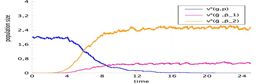
B ​​​​​

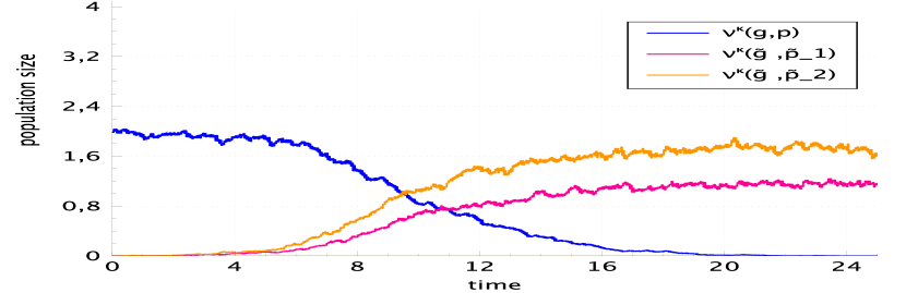
Figure 3. Simulations of the invasion phase with $K=1000$. (A) The mutant phenotype $\tilde{p}_{1}$ has a negative initial growth rate but can switch to $\tilde{p}_{2}$ which has a positive one. The fitness of the genotype $\tilde{g}$ is positive. (B) The fitness of the mutant genotype $\tilde{g}$ is positive, although each phenotype has a negative initial growth rate. This is possible because an outgoing switch is a loss of a cell for a phenotype, but not for the whole genotype.

In example (A), we start with a single mutant carrying trait $(\tilde{g},\tilde{p}_{1})$ and which can switch to $\tilde{p}_{2}$ but the back-switch is relative weak (cf. Tab. 2). According to definition (3.70) we have $f_{(g,p)}(\tilde{g},\tilde{p}_{1})<0$ and $f_{(g,p)}(\tilde{g},\tilde{p}_{2})>0$. However, the global fitness of the genotype $\tilde{g}$ is positive. More precisely, it is given by the largest eigenvalue of $\left(\begin{smallmatrix}-3&2\\ 0.6&1\end{smallmatrix}\right)$, which equals approximatively $1.280$. Therefore, the multi-type branching process approximating the mutant population in the first step is supercritical. This does not depend on the phenotype of the first mutant, i.e.  we would have the same if we had started with a single mutant carrying trait $(\tilde{g},\tilde{p}_{2})$). However, the probability of invasion depends this. In this example, the invasion probability is given by the solution of

$$2y_{1}^{2}+2y_{2}+3-7y_{1} \;=\;0,$$ (3.101)

$$4y_{2}^{2}+0.6y_{1}+2.4-7y_{2} \;=\;0.$$ (3.102)

Thus, if we start with the trait $(\tilde{g},\tilde{p}_{1})$, the invasion probability is approximately $0.199$. Whereas it is $0.338$ if the first one has trait $(\tilde{g},\tilde{p}_{2})$. In Figure 3 (A), the mutant population with genotype $\tilde{g}$ survives and the stochastic process is attracted to the new equilibrium $\mathfrak{n}^{*}((g,p),(\tilde{g},\tilde{p}_{1}),(\tilde{g},\tilde{p}_{2}))\approx(0,0.543,2.554)$, which is a strictly stable.

$b(p)=3$	$d({p})=1$	$c({p},{p})=1$	$c({p},\tilde{p}_{1})=1$	$c(p,\tilde{p}_{2})=0.7$	$s_{\text{ind.}}^{.}(\,.\,,.\,)(.)\equiv 0$	$\nu^{K}_{0}{(g,p)}=2$
$b(\tilde{p}_{1})=2$	$d(\tilde{p}_{1})=1$	$c(\tilde{p}_{1},{p})=1$	$c(\tilde{p}_{1},\tilde{p}_{1})=1$	$c(\tilde{p}_{1},\tilde{p}_{2})=0.5$	$s^{\tilde{g}}(\tilde{p}_{1},\tilde{p}_{2})=2$	$\nu^{K}_{0}{(\tilde{g},\tilde{p}_{1})}=K^{-1}$
$b(\tilde{p}_{2})=4$	$d(\tilde{p}_{2})=1$	$c(\tilde{p}_{2},{p})=0.7$	$c(\tilde{p}_{2},\tilde{p}_{1})=0.5$	$c(\tilde{p}_{2},\tilde{p}_{2})=1$	$s^{\tilde{g}}(\tilde{p}_{2},\tilde{p}_{1})=0.6$	$\nu^{K}_{0}{(\tilde{g},\tilde{p}_{2})}=0$

Table 2. Parameters of Figure 3 (A)

In example (B), $f_{(g,p)}(\tilde{g},\tilde{p}_{1})$ and $f_{(g,p)}(\tilde{g},\tilde{p}_{2})$ are both negative. Nevertheless, the fitness of the genotype is positive and thus the mutant invades with positive probability. (It is given by the largest eigenvalue of $\left(\begin{smallmatrix}-3&2\\ 2&-0.4\end{smallmatrix}\right)$, which equals approximatively $0.685$.) However, the invasion probability is smaller in this example. It is approximately $0.127$ if we start with the trait $(\tilde{g},\tilde{p}_{1})$ and $0.207$ else. In Figure 3 (B), the mutant population survives and the process is attracted to the stable fixed point $\mathfrak{n}^{*}((g,p),(\tilde{g},\tilde{p}_{1}),(\tilde{g},\tilde{p}_{2}))\approx(0,1.153,1.745)$. Hence, this examples illustrate that the usual definition of invasion fitness fails for populations with phenotypic plasticity.

$b(p)=3$	$d({p})=1$	$c({p},{p})=1$	$c({p},\tilde{p}_{1})=1$	$c(p,\tilde{p}_{2})=0.7$	$s_{\text{ind.}}^{.}(\,.\,,.\,)(.)\equiv 0$	$\nu^{K}_{0}{(g,p)}=2$
$b(\tilde{p}_{1})=2$	$d(\tilde{p}_{1})=1$	$c(\tilde{p}_{1},{p})=1$	$c(\tilde{p}_{1},\tilde{p}_{1})=1$	$c(\tilde{p}_{1},\tilde{p}_{2})=0.5$	$s^{\tilde{g}}(\tilde{p}_{1},\tilde{p}_{2})=2$	$\nu^{K}_{0}{(\tilde{g},\tilde{p}_{1})}=1/K$
$b(\tilde{p}_{2})=4$	$d(\tilde{p}_{2})=1$	$c(\tilde{p}_{2},{p})=0.7$	$c(\tilde{p}_{2},\tilde{p}_{1})=0.5$	$c(\tilde{p}_{2},\tilde{p}_{2})=1$	$s^{\tilde{g}}(\tilde{p}_{2},\tilde{p}_{1})=2$	$\nu^{K}_{0}{(\tilde{g},\tilde{p}_{2})}=0$

Table 3. Parameters of Figure 3 (B)

References

- [1] K. B. Athreya. Some results on multitype continuous time Markov branching processes. Ann. Math. Stat., 39:347–357, 1968.
- [2] K. B. Athreya and P. E. Ney. Branching processes. Die Grundlehren der mathematischen Wissenschaften, Vol. 196. Springer-Verlag Berlin Heidelberg, 1972.
- [3] M. Baar, A. Bovier, and N. Champagnat. From stochastic, individual-based models to the canonical equation of adaptive dynamics - in one step. Ann. Appl. Probab., 27:1093–1170, 2016.
- [4] M. Baar, L. Coquille, H. Mayer, M. Hölzel, M. Rogava, T. Tüting, and A. Bovier. A stochastic model for immunotherapy of cancer. Scientific Reports, 6:24169, 2016.
- [5] V. Bansaye and S. Méléard. Stochastic models for structured populations. Scaling limits and long time behavior, volume 1 of Mathematical Biosciences Institute Lecture Series. Stochastics in Biological Systems. Springer, Cham; MBI Mathematical Biosciences Institute, Ohio State University, Columbus, OH, 2015.
- [6] B. Bolker and S. W. Pacala. Using moment equations to understand stochastically driven spatial pattern formation in ecological systems. Theor. Popul. Biol., 52(3):179 – 197, 1997.
- [7] B. M. Bolker and S. W. Pacala. Spatial moment equations for plant competition: understanding spatial strategies and the advantages of short dispersal. Am. Nat., 153(6):575–602, 1999.
- [8] N. Champagnat. A microscopic interpretation for adaptive dynamics trait substitution sequence models. Stoch. Proc. Appl., 116(8):1127–1160, 2006.
- [9] N. Champagnat, P.-E. Jabin, and S. Méléard. Adaptation in a stochastic multi-resources chemostat model. J. Math. Pures Appl., 101(6):755–788, 2014.
- [10] N. Champagnat and S. Méléard. Polymorphic evolution sequence and evolutionary branching. Prob. Theory Rel., 151(1-2):45–94, 2011.
- [11] P. Collet, S. Méléard, and J. A. J. Metz. A rigorous model study of the adaptive dynamics of Mendelian diploids. J. Math. Biol., 67(3):569–607, 2013.
- [12] U. Dieckmann and R. Law. Moment approximations of individual-based models. In U. Dieckmann, R. Law, and J. A. J. Metz, editors, The geometry of ecological interactions: simplifying spatial complexity, pages 252–270. Cambridge University Press, 2000.
- [13] P. Dupuis and R. S. Ellis. A weak convergence approach to the theory of large deviations. Wiley Series in Probability and Statistics. John Wiley & Sons, Inc., New York, 1997.
- [14] S. N. Ethier and T. G. Kurtz. Markov processes. Characterization and convergence. Wiley Series in Probability and Mathematical Statistics. John Wiley & Sons Inc., New York, 1986.
- [15] N. Fournier and S. Méléard. A microscopic probabilistic description of a locally regulated population and macroscopic approximations. Ann. Appl. Probab., 14(4):1880–1919, 2004.
- [16] M. I. Freidlin and A. D. Wentzell. Random perturbations of dynamical systems, volume 260 of Grundlehren der Mathematischen Wissenschaften. Springer, Heidelberg, 3rd edition, 2012.
- [17] M. Hölzel, A. Bovier, and T. Tüting. Plasticity of tumour and immune cells: a source of heterogeneity and a cause for therapy resistance? Nat. Rev. Cancer, 13(5):365–376, 2013.
- [18] H. Kesten and B. P. Stigum. Additional limit theorems for indecomposable multidimensional Galton-Watson processes. Ann. Math. Stat., 37:1463–1481, 1966.
- [19] H. Kesten and B. P. Stigum. A limit theorem for multidimensional Galton-Watson processes. Ann. Math. Stat., 37:1211–1223, 1966.
- [20] H. Kesten and B. P. Stigum. Limit theorems for decomposable multi-dimensional Galton-Watson processes. J. Math. Anal. Appl., 17:309–338, 1967.
- [21] H. Mayer. Contributions to stochastic modelling of the immune system. PhD thesis, Rheinischen Friedrich-Wilhelms-Universität Bonn, Bonn (Germany), 2016.
- [22] S. Pénisson. Conditional limit theorems for multitype branching processes and illustration in epidemiological risk analysis. PhD thesis, Universität Potsdam, Potsdam (Germany), 2010.
- [23] B. A. Sewastjanow. Verzweigungsprozesse. R. Oldenbourg Verlag, Munich-Vienna, 1975.