Standard Steady State Genetic Algorithms Can Hillclimb Faster than Mutation-only Evolutionary Algorithms

Abstract

Explaining to what extent the real power of genetic algorithms lies in the ability of crossover to recombine individuals into higher quality solutions is an important problem in evolutionary computation. In this paper we show how the interplay between mutation and crossover can make genetic algorithms hillclimb faster than their mutation-only counterparts. We devise a Markov Chain framework that allows to rigorously prove an upper bound on the runtime of standard steady state genetic algorithms to hillclimb the OneMax function. The bound establishes that the steady-state genetic algorithms are 25$\%$ faster than all standard bit mutation-only evolutionary algorithms with static mutation rate up to lower order terms for moderate population sizes. The analysis also suggests that larger populations may be faster than populations of size 2. We present a lower bound for a greedy (2+1) GA that matches the upper bound for populations larger than 2, rigorously proving that 2 individuals cannot outperform larger population sizes under greedy selection and greedy crossover up to lower order terms. In complementary experiments the best population size is greater than 2 and the greedy genetic algorithms are faster than standard ones, further suggesting that the derived lower bound also holds for the standard steady state (2+1) GA.

1 Introduction

Genetic algorithms (GAs) rely on a population of individuals that simultaneously explore the search space. The main distinguishing features of GAs from other randomised search heuristics is their use of a population and crossover to generate new solutions. Rather than slightly modifying the current best solution as in more traditional heuristics, the idea behind GAs is that new solutions are generated by recombining individuals of the current population (i.e., crossover). Such individuals are selected to reproduce probabilistically according to their fitness (i.e., reproduction). Occasionally, random mutations may slightly modify the offspring produced by crossover. The original motivation behind these mutations is to avoid that some genetic material may be lost forever, thus allowing to avoid premature convergence [1, 2]. For these reasons the GA community traditionally regards crossover as the main search operator while mutation is considered a “background operator” [2, 3, 4] or a “secondary mechanism of genetic adaptation” [1].

Explaining when and why GAs are effective has proved to be a non-trivial task. Schema theory and its resulting building block hypothesis [1] were devised to explain such working principles. However, these theories did not allow to rigorously characterise the behaviour and performance of GAs. The hypothesis was disputed when a class of functions (i.e., Royal Road), thought to be ideal for GAs, was designed and experiments revealed that the simple (1+1) EA was more efficient [5, 6].

Runtime analysis approaches have provided rigorous proofs that crossover may indeed speed up the evolutionary process of GAs in ideal conditions (i.e., if sufficient diversity is available in the population). The Jump function was introduced by Jansen and Wegener as a first example where crossover considerably improves the expected runtime compared to mutation-only Evolutionary Algorithms (EAs) [7]. The proof required an unrealistically small crossover probability to allow mutation alone to create the necessary population diversity for the crossover operator to then escape the local optimum. Dang et al. recently showed that the sufficient diversity, and even faster upper bounds on the runtime for not too large jump gaps, can be achieved also for realistic crossover probabilities by using diversity mechanisms [8]. Further examples that show the effectiveness of crossover have been given for both artificially constructed functions and standard combinatorial optimisation problems (see the next section for an overview).

Excellent hillclimbing performance of crossover based GAs has been also proved. B. Doerr et al. proposed a (1+($\lambda$,$\lambda$)) GA which optimises the OneMax function in $\Theta(n\sqrt{\log\log\log(n)/\log\log(n)})$ fitness evaluations (i.e., runtime) [9], [10]. Since the unbiased unary black box complexity of OneMax is $\Omega(n\log n)$ [11], the algorithm is asymptotically faster than any unbiased mutation-only evolutionary algorithm (EA). Furthermore, the algorithm runs in linear time when the population size is self-adapted throughout the run [12]. Through this work, though, it is hard to derive conclusions on the working principles of standard GAs because these are very different compared to the (1+($\lambda$,$\lambda$)) GA in several aspects. In particular, the (1+($\lambda$,$\lambda$)) GA was especially designed to use crossover as a repair mechanism that follows the creation of new solutions via high mutation rates. This makes the algorithm work in a considerably different way compared to traditional GAs.

More traditional GAs have been analysed by Sudholt [13]. Concerning OneMax, he shows how ($\mu$+$\lambda$) GAs are twice as fast as their standard bit mutation-only counterparts. As a consequence, he showed an upper bound of $(e/2)n\log n(1+o(1))$ function evaluations for a (2+1) GA versus the $en\log n(1-o(1))$ function evaluations required by any standard bit mutation-only EA [14, 15]. This bound further reduces to $1.19n\ln n\pm O(n\log\log n)$ if the optimal mutation rate is used (i.e., $(1+\sqrt{5})/2\cdot 1/n\approx 1.618/n$). However, the analysis requires that diversity is artificially enforced in the population by breaking ties always preferring genotypically different individuals. This mechanism ensures that once diversity is created on a given fitness level, it will never be lost unless a better fitness level is reached, giving ample opportunities for crossover to exploit this diversity.

Recently, it has been shown that it is not necessary to enforce diversity for standard steady state GAs to outperform standard bit mutation-only EAs [16]. In particular, the Jump function was used as an example to show how the interplay between crossover and mutation may be sufficient for the emergence of the necessary diversity to escape from local optima more quickly. Essentially, a runtime of $O(n^{k-1})$ may be achieved for any sublinear jump length $k>2$ versus the $\Theta(n^{k})$ function evaluations required by standard bit mutation-only EAs.

In this paper, we show that this interplay between mutation and crossover may also speed-up the hillclimbing capabilities of steady state GAs without the need of enforcing diversity artificially. In particular, we consider a standard steady state ($\mu$+1) GA [17, 2, 18] and prove an upper bound on the runtime to hillclimb the OneMax function of $(3/4)en\log n+O(n)$ for any $\mu\geq 3$ and $\mu=o(\log{n}/\log{\log{n}})$ when the standard $1/n$ mutation rate is used. Apart from showing that standard ($\mu$+1) GAs are faster than their standard bit mutation-only counterparts up to population sizes $\mu=o(\log{n}/\log{\log{n}})$, the framework provides two other interesting insights. Firstly, it delivers better runtime bounds for mutation rates that are higher than the standard $1/n$ rate. The best upper bound of $0.72en\log n+O(n)$ is achieved for $c/n$ with $c=\frac{1}{2}\left(\sqrt{13}-1\right)\approx 1.3$. Secondly, the framework provides a larger upper bound, up to lower order terms, for the (2+1) GA compared to that of any $\mu\geq 3$ and $\mu=o(\log{n}/\log{\log{n}})$. The reason for the larger constant in the leading term of the runtime is that, for populations of size 2, there is always a constant probability that any selected individual takes over the population in the next generation. This is not the case for population sizes larger than 2.

To shed light on the exact runtime for population size $\mu=2$ we present a lower bound analysis for a greedy genetic algorithm, which we call (2+1)_S GA, that always selects individuals of highest fitness for crossover and always successfully recombines them if their Hamming distance is greater than 2. This algorithm is similar to the one analysed by Sudholt [13] to allow the derivation of a lower bound, with the exception that we do not enforce any diversity artificially and that our crossover operator is slightly less greedy (i.e., in [13] crossover always recombines correctly individuals also when the Hamming distance is exactly 2). Our analysis delivers a matching lower bound for all mutation rates $c/n$, where $c$ is a constant, for the greedy (2+1)_S GA (thus also $(3/4)en\log n+O(n)$ and $0.72en\log n+O(n)$ respectively for mutation rates $1/n$ and $1.3/n$). This result rigorously proves that, under greedy selection and semi-greedy crossover, the (2+1) GA cannot outperform any ($\mu$+1) GA with $\mu\geq 3$ and $\mu=o(\log{n}/\log{\log{n}})$.

We present some experimental investigations to shed light on the questions that emerge from the theoretical work. In the experiments we consider the commonly used parent selection that chooses uniformly at random from the population with replacement (i.e., our theoretical upper bounds hold for a larger variety of parent selection operators). We first compare the performance of the standard steady state GAs against the fastest standard bit mutation-only EA with fixed mutation rate (i.e., the (1+1) EA [14, 15]) and the GAs that have been proved to outperform it. The experiments show that the speedups over the (1+1) EA occur already for small problem sizes $n$ and that population sizes larger than $2$ are faster than the standard (2+1) GA. Furthermore, the greedy $(2+1)_{S}$ GA indeed appears to be faster than the standard (2+1) GA, further suggesting that the theoretical lower bound also holds for the latter algorithm. Finally, experiments confirm that larger mutation rates than $1/n$ are more efficient. In particular, better runtimes are achieved for mutation rates that are even larger than the ones that minimise our theoretical upper bound (i.e., $c/n$ with 1.5 $\leq c\leq$ 1.6 versus the $c=$1.3 we have derived mathematically; interestingly this experimental rate is similar to the optimal mutation rate for OneMax of the algorithm analysed in [13]). These theoretical and experimental results seem to be in line with those recently presented for the same steady state GAs for the Jump function [16, 8]: higher mutation rates than $1/n$ are also more effective on Jump.

The rest of the paper is structured as follows. In the next section we briefly review previous related works that consider algorithms using crossover operators. In Section 3 we give precise definitions of the steady state ($\mu$+1) GA and of the OneMax function. In Section 4 we present the Markov Chain framework that we will use for the analysis of steady state elitist GAs. In Section 5 we apply the framework to analyse the ($\mu$+1) GA and present the upper bound on the runtime for any $3\leq\mu=o(\log{n}/\log{\log{n}})$ and mutation rate $c/n$ for any constant $c$. In Section 6 we present the matching lower bound on the runtime of the greedy (2+1)_S GA. In Section 7 we present our experimental findings. In the Conclusion we present a discussion and open questions for future work.

2 Related Work

The first rigorous groundbreaking proof that crossover can considerably improve the performance of EAs was given by Jansen and Wegener for the ($\mu$+1) GA with an unrealistically low crossover probability [7]. A series of following works on the analysis of the Jump function have made the algorithm characteristics increasingly realistic [8, 19]. Today it has been rigorously proved that the standard steady state ($\mu$+1) GA with realistic parameter settings does not require artificial diversity enforcement to outperform its standard bit mutation-only counterpart to escape the plateau of local optima of the Jump function [16].

Proofs that crossover may make a difference between polynomial and exponential time for escaping local optima have also been available for some time [20, 6]. The authors devised example functions where, if sufficient diversity was enforced by some mechanism, then crossover could efficiently combine different individuals into an optimal solution. Mutation, on the other hand required a long time because of the great Hamming distance between the local and global optima. The authors chose to call the artificially designed functions Real Royal Road functions because the Royal Road functions devised to support the building block hypothesis had failed to do so [21]. The Real Royal Road functions, though, had no resemblance with the schemata structures required by the building block hypothesis.

The utility of crossover has also been proved for less artificial problems such as coloring problems inspired by the Ising model from physics [22], computing input-output sequences in finite state machines [23], shortest path problems [24], vertex cover [25] and multi-objective optimization problems [26]. The above works show that crossover allows to escape from local optima that have large basins of attraction for the mutation operator. Hence, they establish the usefulness of crossover as an operator to enchance the exploration capabilities of the algorithm.

The interplay between crossover and mutation may produce a speed-up also in the exploitation phase, for instance when the algorithm is hillclimbing. Research in this direction has recently appeared. The design of the (1+($\lambda,\lambda$)) GA was theoretically driven to beat the $\Omega(n\ln n)$ lower bound of all unary unbiased black box algorithms. Since the dynamics of the algorithm differ considerably from those of standard GAs, it is difficult to achieve more general conclusions about the performance of GAs from the analysis of the (1+($\lambda,\lambda$)) GA. From this point of view the work of Sudholt is more revealing when he shows that any standard ($\mu+\lambda$) GA outperforms its standard bit mutation-only counterpart for hillclimbing the OneMax function [13]. The only caveat is that the selection stage enforces diversity artificially, similarly to how Jansen and Wegener had enforced diversity for the Real Royal Road function analysis. In this paper we rigorously prove that it is not necessary to enforce diversity artificially for standard-steady state GAs to outperform their standard bit mutation-only counterpart.

3 Preliminaries

1

2$P\leftarrow\mu\textrm{ individuals, uniformly at random from }\{0,1\}^{n}$;

3 repeat

4       Select $x,y\in P$ with replacement using an operator abiding (1);

5       $z\leftarrow$ Uniform crossover with probability $1/2$ $(x,y)$;

6       Flip each bit in $z$ with probability $c/n$;

7       $P\leftarrow P\cup\{z\}$;

8       Choose one element from $P$ with lowest fitness and remove it from $P$, breaking ties at random;

9until termination condition satisfied;

Algorithm 1 ($\mu$+1) GA [17, 2, 18, 16]

We will analyse the runtime (i.e., the expected number of fitness function evaluations before an optimal search point is found) of a steady state genetic algorithm with population size $\mu$ and offspring size 1 (Algorithm 1). In steady state GAs the entire population is not changed at once, but rather a part of it. In this paper we consider the most common option of creating one new solution per generation [17, 18]. Rather than restricting the algorithm to the most commonly used uniform selection of two parents, we allow more flexibility to the choice of which parent selection mechanism is used. This approach was also followed by Sudholt for the analysis of the ($\mu$+1) GA with diversity [13]. In each generation the algorithm picks two parents from its population with replacement using a selection operator that satisfies the following condition.

$$\forall x,y:\;f(x)\geq f(y)\implies\Pr(\text{select }x)\geq\Pr(\text{select }y).$$ (1)

The condition allows to use most of the popular parent selection mechanisms with replacement such as fitness proportional selection, rank selection or the one commonly used in steady state GAs, i.e., uniform selection [2]. Afterwards, uniform crossover between the selected parents (i.e., each bit of the offspring is chosen from each parent with probability $1/2$) provides an offspring to which standard bit mutation (i.e., each bit is flipped with with probability $c/n$) is applied. The best $\mu$ among the $\mu+1$ solutions are carried over to the next generation and ties are broken uniformly at random.

In the paper we use the standard convention for naming steady state algorithms: the ($\mu$+1) EA differs from the ($\mu$+1) GA by only selecting one individual per generation for reproduction and applying standard bit mutation to it (i.e., no crossover). Otherwise the two algorithms are identical.

We will analyse Algorithm 1 for the well-studied OneMax function that is defined on bitstrings $x\in\{0,1\}^{n}$ of length $n$ and returns the number of $1$-bits in the string: $\text{\sc OneMax}(x)=\sum_{i=1}^{n}x_{i}$. Here $x_{i}$ is the $i$th bit of the solution $x\in\{0,1\}^{n}$. The OneMax benchmark function is very useful to assess the hillclimbing capabilities of a search heuristic. It displays the characteristic function optimisation property that finding improving solutions becomes harder as the algorithm approaches the optimum. The problem is the same as that of identifying the hidden solution of the Mastermind game where we assume for simplicity that the target string is the one of all 1-bits. Any other target string $z\in\{0,1\}^{n}$ may also be used without loss of generality. If a bitstring is used, then OneMax is equivalent to Mastermind with two colours [27]. This can be generalised to many colours if alphabets of greater size are used [28, 29].

4 Markov Chain Framework

Figure 1: Markov Chain for fitness level $i$.

The recent analysis of the ($\mu$+1) GA for the Jump function shows that the interplay between crossover and mutation may create the diversity required for crossover to decrease the expected time to jump towards the optimum [16]. At the heart of the proof is the analysis of a random walk on the number of diverse individuals on the local optima of the function. The analysis delivers improved asymptotic expected runtimes of the ($\mu$+1) GA over mutation-only EAs only for population sizes $\mu=\omega(1)$. This happens because, for larger population sizes, it takes more time to lose diversity once created, hence crossover has more time to exploit it. For OneMax the technique delivers worse asymptotic bounds for population sizes $\mu=\omega(1)$ and an $O(n\ln n)$ bound for constant population size. Hence, the techniques of [16] cannot be directly applied to show a speed-up of the ($\mu$+1) GA over mutation-only EAs and a careful analysis of the leading constant in the runtime is necessary. In this section we present the Markov chain framework that we will use to obtain the upper bounds on the runtime of the elitist steady state GAs. We will afterwards discuss how this approach builds upon and generalises Sudholt’s approach in [13].

The OneMax function has $n+1$ distinct fitness values. We divide the search space into the following canonical fitness levels [30, 31]:

$$L_{i}=\{x\in\{0,1\}^{n}|\text{\sc OneMax}(x)=i\}.$$

We say that a population is in fitness level $i$ if and only if its best solution is in level $L_{i}$.

We use a Markov chain (MC) for each fitness level $i$ to represent the different states the population may be in before reaching the next fitness level. The MC depicted in Fig. 1 distinguishes between states where the population has no diversity (i.e., all individuals have the same genotype), hence crossover is ineffective, and states where diversity is available to be exploited by the crossover operator. The MC has one absorbing state and two transient states. The first transient state $S_{1,i}$ is adopted if the whole population consists of copies of the same individual at level $i$ (i.e., all the individuals have the same genotype). The second state $S_{2,i}$ is reached if the population consists of $\mu$ individuals in fitness level $i$ and at least two individuals $x$ and $y$ are not identical. The second transient state $S_{2,i}$ differs from the state $S_{1,i}$ in having diversity which can be exploited by the crossover operator. $S_{1,i}$ and $S_{2,i}$ are mutually accessible from each other since the diversity can be introduced at state $S_{1,i}$ via mutation with some probability $p_{d}$ and can be lost at state $S_{2,i}$ with some relapse probability $p_{r}$ when copies of a solution take over the population.

The absorbing state $S_{3,i}$ is reached when a solution at a better fitness level is found, an event that happens with probability $p_{m}$ when the population is at state $S_{1,i}$ and with probability $p_{c}$ when the population is at state $S_{2,i}$. We pessimistically assume that in $S_{2,i}$ there is always only one single individual with a different genotype (i.e., with more than one distinct individual, $p_{c}$ would be higher and $p_{r}$ would be zero). Formally when $S_{3,i}$ is reached the population is no longer in level $i$ because a better fitness level has been found. However, we will bound the expected time to reach the absorbing state for the next level only when the whole population has reached it (or a higher level). We do this because we assume that initially all the population is in level $i$ when calculating the transition probabilities in the MC for each level $i$. This implies that bounding the expected times to reach the absorbing states of each fitness level is not sufficient to achieve an upper bound on the total expected runtime. When $S_{3,i}$ is reached for the first time, the population only has one individual at the next fitness level or in a higher one. Only when all the individuals have reached level $i+1$ (i.e., either in state $S_{1,i+1}$ or $S_{2,i+1}$) may we use the MC to bound the runtime to overcome level $i+1$. Then the MC can be applied, once per fitness level, to bound the total runtime until the optimum is reached.

The main distinguishing aspect between the analysis presented herein and that of Sudholt [13] is that we take into account the possibility to transition back and forth (i.e., resp. with probability $p_{d}$ and $p_{r}$) between states $S_{1,i}$ and $S_{2,i}$ as in standard steady state GAs (see Fig. 1). By enforcing that different genotypes on the same fitness level are kept in the population, the genetic algorithm considered in [13] has a good probability of exploiting this diversity to recombine the different individuals. In particular, once the diversity is created it will never be lost, giving many opportunities for crossover to take advantage of it. A crucial aspect is that the probability of increasing the number of ones via crossover is much higher than the probability of doing so via mutation once many 1-bits have been collected. Hence, by enforcing that once State $S_{2,i}$ is reached it cannot be left until a higher fitness level is found, Sudholt could prove that the resulting algorithm is faster compared to only using standard bit mutation. In the standard steady state GA, instead, once the diversity is created it may subsequently be lost before crossover successfully recombines the diverse individuals. This behaviour is modelled in the MC by considering the relapse probability $p_{r}$. Hence, the algorithm spends less time in state $S_{2,i}$ compared to the GA with diversity enforcement. Nevertheless, it will still spend some optimisation time in state $S_{2,i}$ where it will have a higher probability of improving its fitness by exploiting the diversity via crossover than when in state $S_{1,i}$ (i.e., no diversity) where it has to rely on mutation only. For this reason the algorithm will not be as fast for OneMax as the GA with enforced diversity but will still be faster than standard bit mutation-only EAs.

An interesting consequence of the possibility of losing diversity, is that populations of size greater than 2 can be beneficial. In particular the diversity (i.e., State $S_{2,i}$) may be completely lost in the next step when there is only one diverse individual left in the population. When this is the case, the relapse probability $p_{r}$ decreases with the population size $\mu$ because the probability of selecting the diverse individual for removal is $1/\mu$. Furthermore, for population size $\mu=2$ there is a positive probability that diversity is lost in every generation by either of the two individuals taking over, while for larger population sizes this is not the case. As a result our MC framework analysis will deliver a better upper bound for $\mu>2$ compared to the bound for $\mu=2$. This interesting insight into the utility of larger populations could not be seen in the analysis of [13] because there, once the diversity is achieved, it cannot be lost.

We first concentrate on the expected absorbing time of the MC. Afterwards we will calculate the takeover time before we can transition from one MC to the next. Since it is not easy to derive the exact transition probabilities, a runtime analysis is considerably simplified by using bounds on these probabilities. The main result of this section is stated in the following theorem that shows that we can use lower bounds on the transition probabilities moving in the direction of the absorbing state (i.e., $p_{m}$, $p_{d}$ and $p_{c}$) and an upper bound on the probability of moving in the opposite direction to no diversity (i.e., $p_{r}$) to derive an upper bound on the expected absorbing time of the Markov chain. In particular, we define a Markov chain $M^{\prime}$ that uses the bounds on the exact transition probabilities and show that its expected absorbing time is greater than the absorbing time of the original chain. Hereafter, we drop the level index $i$ for brevity and use $E[T_{1}]$ and $E[T_{2}]$ instead of $E[T_{1,i}]$ and $E[T_{2,i}]$ (Similarly, $S_{1}$ will denote state $S_{1,i}$).

Theorem 1.

Consider two Markov chains $M$ and $M^{\prime}$ with the topology in Figure 1 where the transition probabilities for $M$ are $p_{c}$, $p_{m}$, $p_{d}$ , $p_{r}$ and the transition probabilities for $M^{\prime}$ are $p_{c}^{\prime}$, $p_{m}^{\prime}$, $p_{d}^{\prime}$ and $p_{r}^{\prime}$. Let the expected absorbing time for $M$ be $E[T]$ and the expected absorbing time of $M^{\prime}$ starting from state $S_{1}$ be $E[T_{1}^{\prime}]$ respectively. If

• $p_{m}<p_{c}$

• $p_{d}^{\prime}\leq p_{d}$

• $p_{r}^{\prime}\geq p_{r}$

• $p_{c}^{\prime}\leq p_{c}$

• $p_{m}^{\prime}\leq p_{m}$

Then $E[T]\leq E[T_{1}^{\prime}]\leq\frac{p_{c}^{\prime}+p_{r}^{\prime}}{p_{c}^{\prime}p_{d}^{\prime}+p_{c}^{\prime}p_{m}^{\prime}+p_{m}^{\prime}p_{r}^{\prime}}+\frac{1}{p_{c}^{\prime}}$.

We first concentrate on the second inequality in the statement of the theorem which will follow immediately from the next lemma. It allows us to obtain the expected absorbing time of the MC if the exact values for the transition probabilities are known. In particular, the lemma establishes the expected times $E[T_{1}]$ and $E[T_{2}]$ to reach the absorbing state, starting from the states $S_{1}$ and $S_{2}$ respectively.

Lemma 2.

The expected times $E[T_{1}]$ and $E[T_{2}]$ to reach the absorbing state, starting from state $S_{1}$ and $S_{2}$ respectively are as follows:

$$E[T_{1}] =\frac{p_{c}+p_{r}+p_{d}}{p_{c}p_{d}+p_{c}p_{m}+p_{m}p_{r}}\leq\frac{p_{c}+p_{r}}{p_{c}p_{d}+p_{c}p_{m}+p_{m}p_{r}}+\frac{1}{p_{c}}$$

$$E[T_{2}] =\frac{p_{m}+p_{r}+p_{d}}{p_{c}p_{d}+p_{c}p_{m}+p_{m}p_{r}}.$$

Proof.

We analyse the MC and using the law of total expectation together with the conditional probabilities we establish the following recurrence equations:

$$E[T_{1}] =(E[T_{2}]+1)p_{d}+p_{m}+(1+E[T_{1}])(1-p_{d}-p_{m})$$

$$E[T_{2}] =(E[T_{1}]+1)p_{r}+p_{c}+(1+E[T_{2}])(1-p_{c}-p_{r}).$$

We start by solving the system of equations for the Markov chain. In order to get an expression for $E[T_{1}]$, we will first express $E[T_{2}]$ in terms of $E[T_{1}]$.

$$E[T_{2}]=(E[T_{1}]+1)p_{r}+p_{c}+(1+E[T_{2}])(1-p_{c}-p_{r}),$$

implying

$$E[T_{2}]=\frac{(E[T_{1}]+1)p_{r}-p_{r}+1}{p_{c}+p_{r}}=\frac{p_{r}E[T_{1}]+1}{p_{c}+p_{r}}.$$

We now substitute the expression for $E[T_{2}]$ into the equation for $E[T_{1}]$:

$$E[T_{1}] =\left(\frac{p_{r}E[T_{1}]+1}{p_{c}+p_{r}}+1\right)p_{d}+p_{m}+(1+E[T_{1}])(1-p_{d}-p_{m}).$$

Hence,

$$E[T_{1}]=\frac{p_{c}+p_{d}+p_{r}}{p_{c}p_{d}+p_{c}p_{m}+p_{m}p_{r}}.$$

The expression for $E[T_{1}]$ can be bounded from above by separating the $p_{d}$ term in the numerator:

$$E[T_{1}] =\frac{p_{c}+p_{r}}{p_{c}p_{d}+p_{c}p_{m}+p_{m}p_{r}}+\frac{p_{d}}{p_{c}p_{d}+p_{c}p_{m}+p_{m}p_{r}}$$

$$\leq\frac{p_{c}+p_{r}}{p_{c}p_{d}+p_{c}p_{m}+p_{m}p_{r}}+\frac{p_{d}}{p_{c}p_{d}}$$

$$\leq\frac{p_{c}+p_{r}}{p_{c}p_{d}+p_{c}p_{m}+p_{m}p_{r}}+\frac{1}{p_{c}}.$$

If we substitute the value of $E[T_{1}]$ in the above expression for $E[T_{2}]$ we obtain:

$$E[T_{2}] =\frac{\frac{p_{r}(p_{c}+p_{d}+p_{r})}{p_{c}p_{d}+p_{c}p_{m}+p_{m}p_{r}}+1}{p_{c}+p_{r}}$$

$$=\frac{p_{r}(p_{c}+p_{d}+p_{r})+p_{c}p_{d}+p_{c}p_{m}+p_{m}p_{r}}{(p_{c}+p_{r})(p_{c}p_{d}+p_{c}p_{m}+p_{m}p_{r})}$$

$$=\frac{p_{c}(p_{m}+p_{r}+p_{d})+p_{r}(p_{m}+p_{r}+p_{d})}{(p_{c}+p_{r})(p_{c}p_{d}+p_{c}p_{m}+p_{m}p_{r})}$$

$$=\frac{p_{m}+p_{r}+p_{d}}{p_{c}p_{d}+p_{c}p_{m}+p_{m}p_{r}}.$$

∎

Before we prove the first inequality in the statement of Theorem 1, we will derive some helper propositions. We first show that as long as the transition probability of reaching the absorbing state from the state $S_{2}$ (with diversity) is greater than that of reaching the absorbing state from the state with no diversity $S_{1}$ (i.e., $p_{m}<p_{c}$), then the expected absorbing time from state $S_{1}$ is at least as large as the expected time unconditional of the starting point. This will allow us to achieve a correct upper bound on the runtime by just bounding the absorbing time from state $S_{1}$. In particular, it allows us to pessimistically assume that the algorithm starts each new fitness level in state $S_{1}$ (i.e., there is no diversity in the population).

Proposition 3.

Consider a Markov chain with the topology given in Figure 1. Let $E[T_{1}]$ and $E[T_{2}]$ be the expected absorbing times starting from state $S_{1}$ and $S_{2}$ respectively. If $p_{m}<p_{c}$, then $E[T_{1}]>E[T_{2}]$ and $E[T]$, the unconditional expected absorbing time, satisfies $E[T]\leq E[T_{1}]$.

Proof.

From Lemma 2,

$$E[T_{1}] =\frac{p_{c}+p_{d}+p_{r}}{p_{c}p_{d}+p_{c}p_{m}+p_{m}p_{r}}$$

$$E[T_{2}] =\frac{p_{m}+p_{d}+p_{r}}{p_{c}p_{d}+p_{c}p_{m}+p_{m}p_{r}}.$$

Since the denominators in both expressions are the same, $E[T_{1}]>E[T_{2}]$ follows from $p_{c}+p_{d}+p_{r}>p_{m}+p_{d}+p_{r}$, which in turn follows from $p_{c}>p_{m}$. The unconditional expected absorbing time is calculated as the weighted sum $E[T]=p\cdot E[T_{1}]+(1-p)\cdot E[T_{2}]$ where $p$ is the probability that the initial state is $S_{1}$ and $1-p$ is the probability that the initial state is $S_{2}$. Since $E[T_{1}]\geq E[T_{2}]$, the weighted sum $E[T]$ is also smaller than or equal to $E[T_{1}]$. ∎

In the following proposition we show that if we overestimate the probability of losing diversity and underestimate the probability of increasing it, then we achieve an upper bound on the expected absorbing time as long as $p_{m}<p_{c}$. Afterwards, in Proposition 5 we show that an upper bound on the absorbing time is also achieved if the probabilities $p_{c}$ and $p_{m}$ are underestimated.

Proposition 4.

Consider two Markov chains $M$ and $M^{\prime}$ with the topology in Figure 1 where the transition probabilities for $M$ are $p_{c}$, $p_{m}$, $p_{d}$, $p_{r}$ and the transition probabilities for $M^{\prime}$ are $p_{c}$, $p_{m}$, $p_{d}^{\prime}$ and $p_{r}^{\prime}$. Let the expected absorbing times starting from state $S_{1}$ for $M$ and $M^{\prime}$ be $E[T_{1}]$ and $E[T_{1}^{\prime}]$ respectively. If $p_{d}^{\prime}\leq p_{d}$, $p_{r}^{\prime}\geq p_{r}$ and $p_{m}<p_{c}$, then $E[T_{1}]\leq E[T_{1}^{\prime}]$.

Proof.

Let $r$ and $d$ be non-negative slack variables such that $p_{d}^{\prime}=p_{d}-d$, $p_{r}^{\prime}=p_{r}+r$. We prove the claim that the absorbing times

$$E[T_{1}] =\frac{p_{c}+p_{d}+p_{r}}{p_{c}p_{d}+p_{c}p_{m}+p_{m}p_{r}},$$

$$E[T_{1}^{\prime}] =\frac{p_{c}+(p_{d}-d)+(p_{r}+r)}{p_{c}(p_{d}-d)+p_{c}p_{m}+p_{m}(p_{r}+r)},$$

satisfy

$$E[T_{1}^{\prime}]-E[T_{1}]\geq 0.$$

For readability purposes let $A=p_{c}+p_{d}+p_{r}$ and $B=p_{c}p_{d}+p_{c}p_{m}+p_{m}p_{r}$. Then,

$$E[T_{1}^{\prime}] =\frac{p_{c}+p_{d}+p_{r}-d+r}{p_{c}p_{d}+p_{c}p_{m}+p_{m}p_{r}-p_{c}d+p_{m}r}$$

$$=\frac{A+(r-d)}{B-p_{c}d+p_{m}r},$$

$$E[T_{1}^{\prime}]-E[T_{1}] =\frac{A+(r-d)}{B-p_{c}d+p_{m}r}-\frac{A}{B}$$

$$=\frac{Br-Bd+Ap_{c}d-Ap_{m}r}{B(B-p_{c}d+p_{m}r)}.$$

Since the denominator is the product of the denominators of $E[T_{1}^{\prime}]$ and $E[T_{1}]$, we already know that it is positive. We now show that:

$$Br-Bd+Ap_{c}d-Ap_{m}r\geq 0.$$

If we insert the values of $A$ and $B$ we obtain:

$$Br-Bd+Ap_{c}d-Ap_{m}r =(p_{c}p_{d}+p_{c}p_{m}+p_{m}p_{r})r-(p_{c}p_{d}+p_{c}p_{m}+p_{m}p_{r})d$$

$$+(p_{c}+p_{d}+p_{r})p_{c}d-(p_{c}+p_{d}+p_{r})p_{m}r$$

$$= p_{c}p_{d}r-p_{c}p_{m}d-p_{m}p_{r}d+p_{c}^{2}d+p_{r}p_{c}d-p_{d}p_{m}r$$

$$= p_{d}r(p_{c}-p_{m})+p_{c}d(p_{c}-p_{m})+p_{r}d(p_{c}-p_{m}).$$

According to our assumption $p_{c}-p_{m}>0$ the proposition follows because the probabilities and slack variables are non-negative. ∎

Proposition 5.

Consider two Markov chains $M$ and $M^{\prime}$ with the topology in Figure 1 where the transition probabilities for $M$ are $p_{c}$, $p_{m}$, $p_{d}$, $p_{r}$ and the transition probabilities for $M^{\prime}$ are $p_{c}^{\prime}$, $p_{m}^{\prime}$, $p_{d}$ and $p_{r}$. Let the expected absorbing times starting from state $S_{1}$ for $M$ and $M^{\prime}$ be $E[T_{1}]$ and $E[T_{1}^{\prime}]$ respectively. If $p_{c}^{\prime}\leq p_{c}$ and $p_{m}^{\prime}\leq p_{m}$, then $E[T_{1}]\leq E[T_{1}^{\prime}]$.

Proof.

Let $c$ and $m$ be non-negative slack variables such that $p_{c}^{\prime}+c=p_{c}$, $p_{m}^{\prime}+m=p_{m}$. Similarly to the proof of Proposition 4, we prove the claim that the absorbing times

$$E[T_{1}^{\prime}] =\frac{p_{c}^{\prime}+p_{d}+p_{r}}{p_{c}^{\prime}p_{d}+p_{c}^{\prime}p_{m}^{\prime}+p_{m}^{\prime}p_{r}},$$

$$E[T_{1}] =\frac{(p_{c}^{\prime}+c)+p_{d}+p_{r}}{(p_{c}^{\prime}+c)p_{d}+(p_{c}^{\prime}+c)(p_{m}^{\prime}+m)+(p_{m}^{\prime}+m)p_{r}},$$

satisfy

$$E[T_{1}^{\prime}]-E[T_{1}]\geq 0.$$

Again for readability purposes let $A=p_{c}^{\prime}+p_{d}+p_{r}$ and $B=p_{c}^{\prime}p_{d}+p_{c}^{\prime}p_{m}^{\prime}+p_{m}^{\prime}p_{r}$. Then,

$$E[T_{1}^{\prime}]-E[T_{1}]=\frac{A}{B}-\frac{A+c}{B+cp_{d}+p_{c}^{\prime}m+cp_{m}^{\prime}+cm+mp_{r}}$$

$$= \frac{Acp_{d}+Ap_{c}^{\prime}m+Acp_{m}^{\prime}+Acm+Amp_{r}-Bc}{B(B+cp_{d}+p_{c}^{\prime}m+cp_{m}^{\prime}+cm+mp_{r})}.$$

Since the denominator is positive we focus on proving that the numerator ($N$) is also positive

$$N=Acp_{d}+Ap_{c}^{\prime}m+Acp_{m}^{\prime}+Acm+Amp_{r}-Bc\geq 0.$$

Substituting the actual values for $A$ and $B$, we obtain the following equivalent expression:

$$N= (p_{c}^{\prime}+p_{d}+p_{r})cp_{d}+(p_{c}^{\prime}+p_{d}+p_{r})p_{c}^{\prime}m$$

$$+(p_{c}^{\prime}+p_{d}+p_{r})cp_{m}^{\prime}+(p_{c}^{\prime}+p_{d}+p_{r})cm$$

$$+(p_{c}^{\prime}+p_{d}+p_{r})mp_{r}-(p_{c}^{\prime}p_{d}+p_{c}^{\prime}p_{m}^{\prime}+p_{m}^{\prime}p_{r})c$$

$$= (p_{d}+p_{r})cp_{d}+(p_{c}^{\prime}+p_{d}+p_{r})p_{c}^{\prime}m$$

$$+(p_{d}+p_{r})cp_{m}^{\prime}+(p_{c}^{\prime}+p_{d})cm+(p_{c}^{\prime}+p_{d}+p_{r})mp_{r}.$$

Since all of the above terms are positive the proposition follows.

∎

The propositions use that by lower bounding $p_{d}$ and upper bounding $p_{r}$ we overestimate the expected number of generations the population is in state $S_{1}$ compared to the time spent in state $S_{2}$. Hence, if $p_{c}>p_{m}$ we can safely use a lower bound for $p_{d}$ and an upper bound for $p_{r}$ and still obtain a valid upper bound on the runtime $E[T_{1}]$. This is rigorously shown by combining together the results of the previous propositions to prove the main result i.e., Theorem 1.

Proof of Theorem 1.

Consider a third Markov chain $M^{*}$ whose transition probabilities are $p_{c}$, $p_{m}$, $p_{r}^{\prime}$, $p_{d}^{\prime}$. Let the absorbing time of $M$ starting from state $S_{1}$ be $E[T_{1}]$. In order to prove the above statement we will prove the following sequence of inequalities.

$$E[T]\leq E[T_{1}]\leq E[T_{1}^{*}]\leq E[T_{1}^{\prime}].$$

According to Proposition 3, $E[T]\leq E[T_{1}]$ since $p_{c}>p_{m}$. According to Proposition 4 $E[T_{1}]\leq E[T_{1}^{*}]$ since $p_{d}^{\prime}\leq p_{d}$, $p_{r}^{\prime}\geq p_{r}$ and $p_{c}>p_{m}$. Finally, according to Proposition 5, $p_{c}^{\prime}\leq p_{c}$ and $p_{m}^{\prime}\leq p_{m}$ implies $E[T_{1}^{*}]\leq E[T_{1}^{\prime}]$ and our proof is completed by using Lemma 2 to show that the last inequality of the statement holds. ∎

The algorithm may skip some levels or a new fitness level may be found before the whole population has reached the current fitness level. Hence, by summing up the expected runtimes to leave each of the $n+1$ levels and the expected times for the whole population to takeover each level, we obtain an upper bound on the expected runtime. The next lemma establishes an upper bound on the expected time it takes to move from the absorbing state of the previous Markov chain ($S_{3,i}$) to any transient state ($S_{1,i+1}$ or $S_{2,i+1}$) of the next Markov chain. The lemma uses standard takeover arguments originally introduced in the first analysis of the ($\mu$+1) EA for OneMax [32]. To achieve a tight upper bound Witt had to carefully wait for only a fraction of the population to take over a level before the next level was discovered. In our case, the calculation of the transition probabilities of the MC is actually simplified if we wait for the whole population to take over each level. Hence in our analysis the takeover time calculations are more similar to the first analysis of the ($\mu$+1) EA with and without diversity mechanisms to takeover the local optimum of TwoMax [33].

Lemma 6.

Let the best individual of the current population be in level $i$ and all individuals be in level at least $i-1$. Then, the expected time for the whole population to be in level at least $i$ is $\mathcal{O}(\mu\log{\mu})$.

Proof.

Let $k$ be the number of individuals of the population at fitness level $i$. Assume that one these $k$ solutions is selected as a parent. If the other parent is also on level $i$ but has a different genotype, then the Hamming distance between the parents is equal to $2d$ for some $d\in\mathbb{N}$ and the number of $1$-bits in the outcome of the crossover operator is $i-d$ plus a binomially distributed random variable with parameters $2d$ and $1/2$. With probability at least $1/2$ this random variable is larger or equal to $d$ due to the symmetry of the binomial distribution. If the other parent is on level $i-1$ then the Hamming distance between parents is $2d+1$ while the number of $1$-bits in the outcome of the crossover operator is $i-d-1$ plus a binomially distributed random variable with parameters $2d+1$ and $1/2$. The probability that the first $2d$ trials to have an outcome larger than $d$ is $1/2$. On top of that, for the offspring to have $i$ $1$-bits it is necessary that the fitter parent is picked for the final bit position with probability $1/2$. Hence, if at least one $i$ level solution is picked as a parent then with probability at least $1/4$, the outcome of the crossover operator has at least $i$ $1$-bits. If the following mutation does not flip any bits, then a new solution with $i$ or more $1$-bits is added to the population. The solution will be accepted by selection unless the population has already been taken over. The probability that a solution at level $i$ is picked as a parent is at least $2k/\mu$ and the probability that mutation does not flip any bits is $(1-c/n)^{n}\geq 1/(e^{c}+1)$. So the expected time between adding the $k$th and the ($k+1$)th $i$-level solution to the population is less than $2(e^{c}+1)(\mu/k)$. By summing over all $k\in\{1,\ldots,\mu-1\}$, we obtain the following upper bound for the whole population to take over level $i$:

$$\sum_{k=1}^{\mu-1}2(e^{c}+1)(\mu/k) \leq 2(e^{c}+1)\mu\sum_{k=1}^{\mu-1}1/k$$

$$\leq 2(e^{c}+1)\mu\cdot{\mathcal{O}}{(\log{\mu})}=\mathcal{O}(\mu\log{\mu}).$$

∎

The lemma shows that, once a new fitness level is discovered for the first time, it takes at most ${\mathcal{O}}(\mu\log{\mu})$ generations until the whole population consists of individuals from the newly discovered fitness level or higher. While the absorption time of the Markov chain might decrease with the population size, for too large population sizes, the upper bound on the expected total take over time will dominate the runtime. As a result the MC framework will deliver larger upper bounds on the runtime unless the expected time until the population takes over the fitness levels is asymptotically smaller than the expected absorption time of all MCs. For this reason, our results will require population sizes of $\mu=o(\log{n}/\log{\log{n}})$, to allow all fitness levels to be taken over in expected $o(n\log{n})$ time such that the latter time does not affect the leading constant of the total expected runtime.

5 Upper Bound

In this section we use the Markov Chain framework devised in Section 4 to prove that the ($\mu$+1) GA is faster than any standard bit mutation-only ($\mu+\lambda$) EA.

In order to satisfy the requirements of Theorem 1, we first show in Lemma 7 that $p_{c}>p_{m}$ if the population is at one of the final $n/(4c(1+e^{c}))$ fitness levels. The lemma also shows that it is easy for the algorithm to reach such a fitness level. Afterwards we bound the transition probabilities of the MC in Lemma 8. We conclude the section by stating and proving the main result, essentially by applying Theorem 1 with the transition probabilities calculated in Lemma 8.

Lemma 7.

For the ($\mu$+1) GA with mutation rate $c/n$ for any constant $c$, if the population is in any fitness level $i>n-n/(4c(1+e^{c}))$, then $p_{c}$ is always larger than $p_{m}$. The expected time for the ($\mu$+1) GA to sample a solution in fitness level $n-n/(4c(1+e^{c}))$ for the first time is $\mathcal{O}(n\mu\log{\mu})$.

Proof.

We consider the probability $p_{c}$. If two individuals on the same fitness level with non-zero Hamming distance $2d$ are selected as parents with probability $p^{\prime}$, then the probability that the crossover operator yields an improved solution is at least (see proof of Theorem 4 in [13]):

$$\Pr(X>d)= \frac{1}{2}\left(1-\Pr(X=d)\right)=\frac{1}{2}\left(1-2^{-2d}{2d\choose d}\right)\geq 1/4,$$ (2)

where $X$ is a binomial random variable with parameters $2d$ and $1/2$ which represents the number of bit positions where the parents differ and which are set to $1$ in the offspring. With probability $(1-c/n)^{n}$ no bits are flipped and the absorbing state is reached. If any individual is selected twice as parent, then the improvement can only be achieved by mutation (i.e., with probability $p_{m}$) since crossover is ineffective. So $p_{c}>p^{\prime}(1/4)(1-c/n)^{n}+(1-p^{\prime})p_{m}$, hence if $p_{m}<p^{\prime}(1/4)(1-c/n)^{n}+(1-p^{\prime})p_{m}$ it follows that $p_{m}<p_{c}$. The condition can be simplified to $p_{m}<(1/4)(1-c/n)^{n}$ with simple algebraic manipulation. For large enough $n$, $(1-c/n)^{n}\geq 1/(1+e^{c})$ and the condition reduces to $p_{m}<1/(4(1+e^{c}))$.

Since $p_{m}<(n-i)c/n$ is an upper bound on the transition probability (i.e., at least one of the zero bits has to flip to increase the OneMax value), the condition is satisfied for $i\geq n-n/(4c(1+e^{c}))$. For any level $i\leq n-n/(4c(1+e^{c}))$, after the take over of the level occurs in ${\mathcal{O}}(\mu\log{\mu})$ expected time, the probability of improving is at least $\Omega(1)$ due to the linear number of $0$-bits that can be flipped. Hence, we can upper bound the total number of generations necessary to reach fitness level $i=n-n/(4c(1+e^{c}))$ by $\mathcal{O}(n\mu\log{\mu})$.

∎

The lemma has shown that $p_{c}>p_{m}$ holds after a linear number of fitness levels have been traversed. Now, we bound the transition probabilities of the Markov chain.

Lemma 8.

Let $\mu\geq 3$. Then the transition probabilities $p_{d}$, $p_{c}$, $p_{r}$ and $p_{m}$ are bounded as follows:

$$p_{d} \geq\frac{\mu}{(\mu+1)}\frac{i(n-i)c^{2}}{n^{2}(e^{c}+{\mathcal{O}}(1/n))}, p_{c}\geq\frac{\mu-1}{2\mu^{2}(e^{c}+{\mathcal{O}}(1/n))},$$

$$p_{r} \leq\frac{(\mu-1)\big{(}2\mu-1+{\mathcal{O}}(1/n)\big{)}}{2e^{c}\mu^{2}(\mu+1)}, p_{m}\geq\frac{c(n-i)}{n(e^{c}+{\mathcal{O}}(1/n))}.$$

Proof.

We first bound the probability $p_{d}$ of transitioning from the state $S_{1,i}$ to the state $S_{2,i}$. In order to introduce a new solution at level $i$ with different genotype, it is sufficient that the mutation operator simultaneously flips one of the $n-i$ 0-bits and one of the $i$ 1-bits while not flipping any other bit. We point out that in $S_{1,i}$, all individuals are identical, hence crossover is ineffective. Moreover, when the diverse solution is created, it should stay in the population, which occurs with probability $\mu/(\mu+1)$ since one of the $\mu$ copies of the majority individual should be removed by selection instead of the offspring. So $p_{d}$ can be lower bounded as follows:

$$p_{d} \geq\frac{\mu}{(\mu+1)}\frac{ic}{n}\frac{(n-i)c}{n}\left(1-\frac{c}{n}\right)^{n-2}.$$

Using the inequality $(1-1/x)^{x-1}\geq 1/e\geq(1-1/x)^{x}$ , we now bound $\left(1-\frac{c}{n}\right)^{n-2}$ as follows:

$$\left(1-\frac{c}{n}\right)^{n-2} \geq\left(1-\frac{c}{n}\right)^{n-1}\geq\left(1-\frac{c}{n}\right)^{n}$$

$$=\bigg{(}\left(1-\frac{c}{n}\right)^{(n/c)-1}\left(1-\frac{c}{n}\right)\bigg{)}^{c}$$

$$\geq\bigg{(}\frac{1}{e}\left(1-\frac{c}{n}\right)\bigg{)}^{c}\geq\frac{1}{e^{c}}\left(1-\frac{c^{2}}{n}\right),$$

where in the last step we used the Bernoulli’s inequality.

We can further absorb the $c^{2}/n$ in an asymptotic ${\mathcal{O}}(1/n)$ term as follows:

$$\left(1-\frac{c}{n}\right)^{n-2} \geq\left(1-\frac{c}{n}\right)^{n-1}\geq\left(1-\frac{c}{n}\right)^{n}\geq\frac{1}{e^{c}}\left(1-\frac{c^{2}}{n}\right)$$

$$\geq e^{-c}-{\mathcal{O}}(1/n)=\frac{1}{e^{c}+{\mathcal{O}}(1/n)}.$$ (3)

The bound for $p_{d}$ is then,

$$p_{d} \geq\frac{\mu}{(\mu+1)}\frac{i(n-i)c^{2}}{n^{2}\big{(}e^{c}+{\mathcal{O}}(1/n)\big{)}}.$$

We now consider $p_{c}$. To transition from state $S_{2,i}$ to $S_{3,i}$ (i.e., $p_{c}$) it is sufficient that two genotypically different individuals are selected as parents (i.e., with probability at least $2(\mu-1)/\mu^{2}$), that crossover provides a better solution (i.e., with probability at least $1/4$ according to Eq. (2)) and that mutation does not flip any bits (i.e., probability $(1-c/n)^{n}\geq 1/\big{(}e^{c}+{\mathcal{O}}(1/n)\big{)}$ according to Eq. (3)). Therefore, the probability is

$$p_{c} \geq 2\frac{\mu-1}{\mu^{2}}\frac{1}{4}\left(1-\frac{c}{n}\right)^{n}\geq\frac{\mu-1}{2\mu^{2}(e^{c}+{\mathcal{O}}(1/n))}$$

For calculating $p_{r}$ we pessimistically assume that the Hamming distance between the individuals in the population is 2 and that there is always only one individual with a different genotype. A population in state $S_{2,i}$ which has diversity, goes back to state $S_{1,i}$ when:

1. A majority individual is selected twice as parent (i.e., probability $(\mu-1)^{2}/\mu^{2})$, mutation does not flip any bit (i.e., probability $(1-c/n)^{n}$) and the minority individual is discarded (i.e., probability $1/(\mu+1)$).

2. Two different individuals are selected as parents, crossover chooses either from the majority individual in both bit locations where they differ (i,e., prob. 1/4) and mutation does not flip any bit (i.e., probability $(1-c/n)^{n}\leq 1/e^{c}$) or mutation must flip at least one specific bit (i.e., probability $\mathcal{O}(1/n)$). Finally, the minority individual is discarded (i.e., probability $1/(\mu+1)$).

3. A minority individual is chosen twice as parent and the mutation operator flips at least two specific bit positions (i.e., with probability ${\mathcal{O}}(1/n^{2})$) and finally the minority individual is discarded (i.e., probability $1/(\mu+1)$).

Hence, the probability of losing diversity is:

$$p_{r} \leq\frac{1}{\mu+1}\bigg{[}\frac{(\mu-1)^{2}}{\mu^{2}}\left(1-\frac{c}{n}\right)^{n}+2\frac{1}{\mu}\frac{\mu-1}{\mu}\left(\frac{1}{4}\left(1-\frac{c}{n}\right)^{n}+\mathcal{O}(1/n)\right)+{\mathcal{O}}(1/n^{2})\bigg{]}$$

$$\leq\frac{2(\mu-1)^{2}+(\mu-1)+4e^{c}(\mu-1){\mathcal{O}}(1/n)}{2e^{c}\mu^{2}(\mu+1)}+\frac{{\mathcal{O}}(1/n^{2})}{\mu+1}$$

$$=\frac{(\mu-1)[2(\mu-1)+1+4e^{c}{\mathcal{O}}(1/n)]+2e^{c}\mu^{2}{\mathcal{O}}(1/n^{2})}{2e^{c}\mu^{2}(\mu+1)}$$

$$=\frac{(\mu-1)[2(\mu-1)+1+{\mathcal{O}}(1/n)]+{\mathcal{O}}(1/n^{2})}{2e^{c}\mu^{2}(\mu+1)}$$

$$\leq\frac{(\mu-1)(2\mu-1+\mathcal{O}(1/n))}{2e^{c}\mu^{2}(\mu+1)}.$$

In the last inequality we absorbed the ${\mathcal{O}}(1/n^{2})$ term into the ${\mathcal{O}}(1/n)$ term.

The transition probability $p_{m}$ from state $S_{1,i}$ to state $S_{3,i}$ is the probability of improvement by mutation only, because crossover is ineffective at state $S_{1,i}$. The number of 1-bits in the offspring increases if the mutation operator flips one of the $(n-i)$ 0-bits ( i.e., with probability $c(n-i)/n$) and does not flip any other bit (i.e., with probability $(1-c/n)^{n-1}\geq\big{(}e^{c}+{\mathcal{O}}(1/n)\big{)}^{-1}$ according to Eq. (3)). Therefore, the lower bound on the probability $p_{m}$ is:

$$p_{m}\geq\frac{c(n-i)}{n\big{(}e^{c}+{\mathcal{O}}(1/n)\big{)}}.$$

∎

We are finally ready to state our main result.

Theorem 9.

The expected runtime of the ($\mu$+1) GA with $\mu\geq 3$ and mutation rate $c/n$ for any constant $c$ on OneMax is:

$$E[T]\leq\frac{3e^{c}n\log{n}}{c(3+c)}+{\mathcal{O}}{(n\mu\log{\mu})}.$$

For $\mu=o(\log{n}/\log{\log{n}})$, the bound reduces to:

$$E[T]\leq\frac{3}{c(3+c)}e^{c}n\log{n}\left(1+o(1)\right).$$

Proof.

We use Theorem 1 to bound $E[T_{i}]$, the expected time until the ($\mu$+1) GA creates an offspring at fitness level $i+1$ or above given that all individuals in its initial population are at level $i$. The bounds on the transition probabilities established in Lemma 8 will be set as the exact transition probabilities of another Markov chain, $M^{\prime}$, with absorbing time larger than $E[T_{i}]$ (by Theorem 1). Since Theorem 1 requires that $p_{c}>p_{m}$ and Lemma 7 establishes that $p_{c}>p_{m}$ holds for all fitness levels $i>n-n/4c(1+e^{c})$, we will only analyse $E[T_{i}]$ for $n-1\geq i>n-n/\big{(}4c(1+e^{c})\big{)}$. Recall that, by Lemma 7, level $n-n/\big{(}4c(1+e^{c})\big{)}$ is reached in expected ${\mathcal{O}}(n\mu\log{\mu})$ time.

Consider the expected absorbing time $E[T_{i}^{\prime}]$, of the Markov chain $M^{\prime}$ with transition probabilities:

$$p_{d}^{\prime}:=\frac{\mu}{(\mu+1)}\frac{i(n-i)c^{2}}{n^{2}(e^{c}+{\mathcal{O}}(1/n))}, p_{c}^{\prime}:=\frac{\mu-1}{2\mu^{2}(e^{c}+{\mathcal{O}}(1/n))},$$

$$p_{r}^{\prime}:=\frac{(\mu-1)\big{(}2\mu-1+{\mathcal{O}}(1/n)\big{)}}{2e^{c}\mu^{2}(\mu+1)}, p_{m}^{\prime}:=\frac{c(n-i)}{n(e^{c}+{\mathcal{O}}(1/n))}.$$

According to Theorem 1:

$$E[T_{i}]\leq E[T_{i,1}^{\prime}]\leq\frac{p_{c}^{\prime}+p_{r}^{\prime}}{p_{c}^{\prime}p_{d}^{\prime}+p_{c}^{\prime}p_{m}^{\prime}+p_{m}^{\prime}p_{r}^{\prime}}+\frac{1}{p_{c}^{\prime}}.\\$$ (4)

We simplify the numerator and the denominator of the first term separately. The numerator is

$$p_{c}^{\prime}+p_{r}^{\prime} =\frac{\mu-1}{2\mu^{2}(e^{c}+{\mathcal{O}}(1/n))}+\frac{(\mu-1)\big{(}2\mu-1+{\mathcal{O}}(1/n)\big{)}}{2e^{c}\mu^{2}(\mu+1)}$$

$$\leq\frac{\mu-1}{2\mu^{2}e^{c}}\left(1+\frac{2\mu-1+{\mathcal{O}}(1/n)}{\mu+1}\right)\leq\frac{(\mu-1)[3\mu+{\mathcal{O}}(1/n)]}{2\mu^{2}e^{c}(\mu+1)}.$$ (5)

We can also rearrange the denominator $D=p_{c}^{\prime}p_{d}^{\prime}+p_{c}^{\prime}p_{m}^{\prime}+p_{m}^{\prime}p_{r}^{\prime}$ as follows:

$$D =p_{c}^{\prime}(p_{d}^{\prime}+p_{m}^{\prime})+p_{m}^{\prime}p_{r}^{\prime}$$

$$=\frac{(\mu-1)\left(\frac{\mu i(n-i)c^{2}}{(\mu+1)n^{2}\left(e^{c}+{\mathcal{O}}(1/n)\right)}+\frac{c(n-i)}{n\left(e^{c}+{\mathcal{O}}(1/n)\right)}\right)}{2\mu^{2}\left(e^{c}+{\mathcal{O}}(1/n)\right)}$$

$$\text{ }+\frac{c(n-i)(\mu-1)\big{(}2\mu-1+{\mathcal{O}}(1/n)\big{)}}{n\left(e^{c}+{\mathcal{O}}(1/n)\right)2e^{c}\mu^{2}(\mu+1)}$$

$$\geq\frac{(\mu-1)\left(\frac{\mu i(n-i)c^{2}}{(\mu+1)n^{2}}+\frac{c(n-i)}{n}\right)}{2\mu^{2}\left(e^{2c}+{\mathcal{O}}(1/n)\right)}+\frac{c(n-i)(\mu-1)\big{(}2\mu-1+{\mathcal{O}}(1/n)\big{)}}{n\left(e^{2c}+{\mathcal{O}}(1/n)\right)2\mu^{2}(\mu+1)}$$

$$\geq\frac{c(n-i)(\mu-1)}{2\mu^{2}\left(e^{2c}+{\mathcal{O}}(1/n)\right)}\cdot\left(\frac{\mu ic}{(\mu+1)n^{2}}+\frac{1}{n}+\frac{2\mu-1+{\mathcal{O}}(1/n)}{n(\mu+1)}\right)$$

$$\geq\frac{c(n-i)(\mu-1)}{2\mu^{2}\left(e^{2c}+{\mathcal{O}}(1/n)\right)}\cdot\left(\frac{\mu ic+(\mu+1)n+n\big{(}2\mu-1+{\mathcal{O}}(1/n)\big{)}}{(\mu+1)n^{2}}\right)$$

$$\geq\frac{c(n-i)(\mu-1)\bigg{(}\mu ic+n\bigg{[}3\mu+{\mathcal{O}}(1/n)\bigg{]}\bigg{)}}{2\mu^{2}\left(e^{2c}+{\mathcal{O}}(1/n)\right)(\mu+1)n^{2}}.$$

Note that the term in square brackets is the same in both the numerator (i.e., Eq. (5)) and the denominator (i.e., Eq. (LABEL:eq:dnm)) including the small order terms in ${\mathcal{O}}(1/n)$ (i.e., they are identical). Let $A=[3\mu+c^{\prime}/n]$, where $c^{\prime}>0$ is the smallest constant that satisfies the ${\mathcal{O}}(1/n)$ in the upper bound on $p_{r}$ in Lemma 8. We can now put the numerator and denominator together and simplify the expression :

$$\frac{p_{c}^{\prime}+p_{r}^{\prime}}{p_{c}^{\prime}(p_{d}^{\prime}+p_{m}^{\prime})+p_{m}^{\prime}p_{r}^{\prime}} \leq\frac{(\mu-1)A}{2\mu^{2}e^{c}(\mu+1)}\cdot\frac{2\mu^{2}\left(e^{2c}+{\mathcal{O}}(1/n)\right)(\mu+1)n^{2}}{c(n-i)(\mu-1)(\mu ic+nA)}$$

$$\leq\frac{A\left(e^{2c}+{\mathcal{O}}(1/n)\right)n^{2}}{e^{c}c(n-i)(\mu ic+nA)}.$$

By using that $\frac{e^{2c}+{\mathcal{O}}(1/n)}{e^{c}}\leq e^{c}+{\mathcal{O}}(1/n)$, we get:

$$\frac{p_{c}^{\prime}+p_{r}^{\prime}}{p_{c}^{\prime}(p_{d}^{\prime}+p_{m}^{\prime})+p_{m}^{\prime}p_{r}^{\prime}} \leq\frac{A\left(e^{c}+{\mathcal{O}}(1/n)\right)n^{2}}{c(n-i)(\mu ic+nA)}$$

$$\leq e^{c}\frac{An^{2}}{c(n-i)(\mu ic+nA)}+{\mathcal{O}}(1/n)\frac{An^{2}}{c(n-i)(\mu ic+nA)}.$$

The facts, $n-i\geq 1$, $A=\Omega(1)$, and $\mu,i,c>0$ imply that, $nA+\mu ic=\Omega(n)$ and $\frac{An^{2}}{c(n-i)(\mu ic+nA)}={\mathcal{O}}(n)$. When multiplied by the ${\mathcal{O}}(1/n)$ term, we get:

$$\leq\frac{e^{c}n}{c(n-i)}\frac{An}{(\mu ic+nA)}+{\mathcal{O}}(1).$$

By adding and subtracting $\mu ic$ to the numerator of $\frac{An}{(\mu ic+nA)}$, we obtain:

$$\leq\frac{e^{c}n}{c(n-i)}\left(1-\frac{\mu ic}{\mu ic+nA}\right)+{\mathcal{O}}(1).$$

Note that the multiplier outside the brackets, $(e^{c}n)/(c(n-i))$, is in the order of ${\mathcal{O}}\big{(}n/(n-i)\big{)}$. We now add and subtract $\mu nc$ to the numerator of $-\frac{\mu ic}{\mu ic+nA}$ to create a positive additive term in the order of ${\mathcal{O}}\big{(}\mu(n-i)/n\big{)}$.

$$=\frac{e^{c}n}{c(n-i)}\left(1-\frac{\mu nc}{\mu ic+nA}+\frac{\mu(n-i)c}{\mu ic+nA}\right)+{\mathcal{O}}(1)$$

$$=\frac{e^{c}n}{c(n-i)}\left(1-\frac{\mu nc}{\mu ic+nA}\right)+\frac{e^{c}n}{c(n-i)}\frac{\mu(n-i)c}{\mu ic+nA}+{\mathcal{O}}(1)$$

$$=\frac{e^{c}n}{c(n-i)}\left(1-\frac{\mu nc}{\mu ic+nA}\right)+{\mathcal{O}}(\mu).$$

Since $p_{c}^{\prime}=\Omega(1/\mu)$, we can similarly absorb $1/p_{c}^{\prime}$ into the $\mathcal{O}(\mu)$ term. After the addition of the remaining term $1/p_{c}^{\prime}$ from Eq.(4), we obtain a valid upper bound on $E[T_{i}]$:

$$E[T_{i}] \leq\frac{p_{c}^{\prime}+p_{r}^{\prime}}{p_{c}^{\prime}p_{d}^{\prime}+p_{c}^{\prime}p_{m}^{\prime}+p_{m}^{\prime}p_{r}^{\prime}}+\frac{1}{p_{c}^{\prime}}\leq\frac{e^{c}n}{c(n-i)}\bigg{(}1-\frac{\mu nc}{\mu ic+nA}\bigg{)}+\mathcal{O}(\mu).$$

In order to bound the negative term, we will rearrange its denominator (i.e., $nA+\mu ic$):

$$n\big{[}3\mu+c^{\prime}/n]+\mu ic =3\mu n+c^{\prime}+\mu ic$$

$$=3\mu n+c^{\prime}-(n-i)\mu c+\mu nc$$

$$<\mu n(3+c)+c^{\prime},$$

where the second equality is obtained by adding and subtracting $\mu nc$. Altogether,

$$E[T_{i}] \leq\frac{e^{c}n}{c(n-i)}\bigg{(}1-\frac{\mu nc}{\mu n(3+c)+c^{\prime}}\bigg{)}+\mathcal{O}(\mu)$$

$$=\frac{e^{c}n}{c(n-i)}\bigg{(}1-\frac{\mu nc+c^{\prime}\frac{c}{3+c}-c^{\prime}\frac{c}{3+c}}{\mu n(3+c)+c^{\prime}}\bigg{)}+\mathcal{O}(\mu)$$

$$=\frac{e^{c}n}{c(n-i)}\bigg{(}1-\frac{c}{3+c}+\frac{c^{\prime}\frac{c}{3+c}}{\mu n(3+c)+c^{\prime}}\bigg{)}+\mathcal{O}(\mu)$$

$$=\frac{e^{c}n}{c(n-i)}\bigg{(}1-\frac{c}{3+c}+{\mathcal{O}}(1/n)\bigg{)}+\mathcal{O}(\mu)$$

$$=\frac{e^{c}n}{c(n-i)}\frac{3}{3+c}+\mathcal{O}(\mu).$$

If we add the expected time to take over each fitness level from Lemma 6 and sum over all fitness levels the upper bound on the runtime is:

$$\sum\limits_{i=n-n/(4c(1+e^{c}))}^{n}\bigg{(}\frac{e^{c}n}{c(n-i)}\frac{3}{3+c}+{\mathcal{O}}(\mu)+{\mathcal{O}}{(\mu\log{\mu})}\bigg{)}$$

$$\leq\sum\limits_{i=0}^{n}\bigg{(}\frac{e^{c}n}{c(n-i)}\frac{3}{3+c}+{\mathcal{O}}{(\mu\log{\mu})}\bigg{)}$$

$$\leq\frac{3e^{c}n\log{n}}{c(3+c)}+{\mathcal{O}}{(n\mu\log{\mu})}\leq\frac{3e^{c}n\log{n}}{c(3+c)}\left(1+o(1)\right),$$

where in the last inequality we use $\mu=o(\log{n}/\log{\log{n}})$ to prove the second statement of the theorem. ∎

The second statement of the theorem provides an upper bound of $(3/4)en\log n$ for the standard mutation rate $1/n$ (i.e., $c=1$) and $\mu=o(\log{n}/\log{\log{n}})$. The upper bound is minimised for $c=\frac{1}{2}\left(\sqrt{13}-1\right)$. Hence, the best upper bound is delivered for a mutation rate of about $1.3/n$. The resulting leading term of the upper bound is:

$$E[T]\leq\frac{6e^{\frac{1}{2}\left(\sqrt{13}-1\right)}n\log{n}}{\left(\sqrt{13}-1\right)\left(\frac{1}{2}\left(\sqrt{13}-1\right)+3\right)}\approx 1.97n\log{n}.$$

We point out that Theorem 9 holds for any $\mu\geq 3$. Our framework provides a higher upper bound when $\mu=2$ compared to larger values of $\mu$. The main difference lies in the probability $p_{r}$ as shown in the following lemma.

Lemma 10.

The transition probabilities $p_{m}$, $p_{r}$, $p_{c}$ and $p_{d}$ for the (2+1) GA, with mutation rate $c/n$ and $c$ constant, are bounded as follows:

$$p_{d} \geq\frac{2}{3}\frac{i(n-i)c^{2}}{n^{2}(e^{c}+{\mathcal{O}}(1/n))}, p_{c}\geq\frac{1}{8(e^{c}+{\mathcal{O}}(1/n))},$$

$$p_{r} \leq\frac{5}{24e^{c}}+{\mathcal{O}}(1/n), p_{m}\geq\frac{c(n-i)}{(e^{c}+{\mathcal{O}}(1/n))n}.$$

Proof.

While the other probabilities are obtained by setting $\mu=2$ in the expressions from Lemma 8, the probability of losing diversity is larger for a population of size two than it is for $\mu\geq 3$. When either individual is picked twice as the parent (which occurs with probability $1/2$) and then the offspring is not mutated (which occurs with probability less than $1/e^{c}$), a copy of a solution is introduced into the population. Moreover, a copy can also be introduced if two different genotypes are selected and then crossover picks the same parents for the bit positions where the parents differ, which occurs with probability at most $1/4$. Any other event which produces a copy of one of the individuals requires flipping a constant number of specific bits which occurs with probability ${\mathcal{O}}(1/n)$. Once a copy is added to the population, the diversity is lost if the minority solution is removed from the population which occurs with probability $1/3$. Hence, by putting together the above probabilities we get

$$p_{r}\leq \frac{1}{3}\bigg{(}\frac{1}{2}e^{-c}+\frac{1}{2}\bigg{(}\frac{1}{4}e^{-c}+{\mathcal{O}}(1/n)\bigg{)}\bigg{)}$$

$$\leq \frac{5}{24e^{c}}+{\mathcal{O}}(1/n).$$

∎

The upper bound on $p_{r}$ from Lemma 8 is $1/(8e^{c})$, which is smaller than the bound we have just found. This is due to the assumptions in the lemma that there can be only one genotype in the population at a given time which can take over the population in the next iteration. However, when $\mu=2$, either individual can take over the population in the next iteration. This larger upper bound on $p_{r}$ for $\mu=2$ leads to a larger upper bound on the runtime of $E[T]\leq\frac{4}{c+4}\frac{e^{c}n\log{n}}{c}(1+o(1))$ for the (2+1) GA. The calculations are omitted as they are the same as those of the proof of Theorem 9 where $p_{r}\geq 5/(24e^{c})+{\mathcal{O}}(1/n)$ is used and $\mu$ is set to 2.

6 Lower bound

1

2$P\leftarrow\mu\textrm{ individuals, uniformly at random from }\{0,1\}^{n}$;

3 repeat

4       Choose $x,y\in P$ uniformly at random among $P^{*}$, the individuals with the current best fitness $f^{*}$;

5       $z\leftarrow$ Uniform crossover with probability $1/2$ $(x,y)$;

6       Flip each bit in $z$ with probability $c/n$;

7       If $f(z)=f^{*}$ and $\max\limits_{w\in P^{*}}(HD(w,z))>2$ then $z\leftarrow z\vee\operatorname*{arg\,max}\limits_{w\in P^{*}}(HD(w,z))$ ;

8      

9      $P\leftarrow P\cup\{z\}$;

10      

11      Choose one element from $P$ with lowest fitness and remove it from $P$, breaking ties at random;

12until termination condition satisfied;

Algorithm 2 $(2+1)_{S}$ GA

In the previous section we provided a higher upper bound for the $(2+1)$ GA compared to the $(\mu+1)$ GA with population size greater than 2 and $\mu=o(\log{n}/\log{\log{n}})$. To rigorously prove that the $(2+1)$ GA is indeed slower, we require a lower bound on the runtime of the algorithm that is higher than the upper bound provided in the previous section for the $(\mu+1)$ GA ($\mu\geq 3$).

Since providing lower bounds on the runtime is a notoriously hard task, we will follow a strategy previously used by Sudholt [13] and analyse a version of the ($\mu$+1) GA with greedy parent selection and greedy crossover (i.e., Algorithm 2) in the sense that:

1. Parents are selected uniformly at random only among the solutions from the highest fitness level (greedy selection).

2. If the offspring has the same fitness as its parents and its Hamming distance to any individual with equal fitness in the population is larger than 2, then the algorithm automatically performs an OR operation between the offspring and the individual with the largest Hamming distance and fitness, breaking ties arbitrarily, and adds the resulting offspring to the population i.e., we pessimistically allow it to skip as many fitness levels as possible (semi-greedy crossover).

The greedy selection allows us to ignore the improvements that occur via crossover between solutions from different fitness levels. Thus, the crossover is only beneficial when there are at least two different genotypes in the population at the highest fitness level discovered so far. The difference with the algorithm analysed by Sudholt [13] is that the $(2+1)_{S}$ GA we consider does not use any diversity mechanism and it does not automatically crossover correctly when the Hamming distance between parents is exactly 2. As a result, there still is a non-zero probability of losing diversity before a successful crossover occurs. The crossover operator of the $(2+1)_{S}$ GA is less greedy than the one analysed in [13] (i.e., there crossover is automatically successful also when the Hamming distance between the parents is 2). We point out that the upper bounds on the runtime derived in the previous section also hold for the greedy $(2+1)_{S}$ GA.

The Markov chain structure of Figure 1 is still representative of the states that the algorithm can be in. When there is no diversity in the population, either an improvement via mutation occurs or diversity is introduced into the population by the mutation operator. When diversity is present, both crossover and mutation can reach a higher fitness level while there is also a probability that the population will lose diversity by replicating one of the existing genotypes. With a population size of two the diversity can be lost by creating a copy of either solution and removing the other one from the population during environmental selection (i.e., Line 8 in Algorithm 2). With population sizes greater than two, the loss of diversity can only occur when the majority genotype (i.e., the genotype with most copies in the population) is replicated. Building upon this we will show that the asymptotic performance of $(2+1)_{S}$ GA for OneMax cannot be better than that of the ($\mu$+1) GAs for $\mu>2$.

Like in [13] for our analysis we will apply the fitness level method for lower bounds proposed by Sudholt [14].

Theorem 11.

[14] Consider a partition of the search space into non-empty sets $A_{1},\ldots,A_{m}$. For a search algorithm $\mathcal{A}$, we say that it is in $A_{i}$ or on level $i$ if the best individual created so far is in $A_{i}$ . Let the probability of $\mathcal{A}$ traversing from level $i$ to level $j$ in one step be at most $u_{i}\cdot\gamma_{i,j}$ for all $j>i$ and $\sum_{j=i+1}^{m}\gamma_{i,j}=1$ for all $i$. Assume that for all $j>i$ and some $0\leq\chi\leq 1$ it holds

$$\gamma_{i,j}\geq\chi\sum_{k=j}^{m}\gamma_{i,k}$$

Then the expected hitting time of $A_{m}$ is at least

$$\sum_{i=1}^{m-1}\Pr(\mathcal{A}\text{ starts in }A_{i})\cdot\bigg{(}\frac{1}{u_{i}}+\chi\sum\limits_{j=i+1}^{m-1}\frac{1}{u_{j}}\bigg{)}$$

$$\geq \sum_{i=1}^{m-1}\Pr(\mathcal{A}\text{ starts in }A_{i})\cdot\chi\sum\limits_{j=i}^{m-1}\frac{1}{u_{j}}.$$

Due to the greedy crossover and the greedy parent selection used in [13], the population could be represented by the trajectory of a single individual. If an offspring with lower fitness was added to the population, then the greedy parent selection never chose it. If instead, a solution with equally high fitness and different genotype was created, then the algorithm immediately reduced the population to a single individual that is the best possible outcome from crossing over the two genotypes. The main difference between the following analysis and that of [13] is that we want to take into account the possibility that the gained diversity may be lost before crossover exploits it. To this end, when individuals of equal fitness and Hamming distance 2 are created, crossover only exploits this successfully (i.e., goes to the next fitness level) with the conditional probability that crossover is successful before the diversity is lost. Otherwise, the diversity is lost. Only when individuals of Hamming distance larger than 2 are created, we allow crossover to immediately provide the best possible outcome as in [13].

Now, we can state the main result of this section.

Theorem 12.

The expected runtime of the $(2+1)_{S}$ GA with mutation probability $p=c/n$ for any constant $c$ on OneMax is no less than:

$$\frac{3e^{c}}{c\bigg{(}3+\max\limits_{1\leq k\leq n}(\frac{(np)^{k}}{(k!)^{2}})\bigg{)}}n\log{n}-\mathcal{O}(n\log{\log{n}}).$$

Proof.

To prove the theorem statement we wish to apply Theorem 11. We say that the $(2+1)_{S}$ GA is on level $i$ if its current best solution has $i$ 1-bits. It will suffice to calculate the runtime of the $(2+1)_{S}$ GA starting from fitness level $\ell=\lceil n-\min\{n/\log{n},n/(p^{2}\log{n})\}\rceil$. Given the greedy selection, the algorithm always reaches a new level in state $S_{1}$ (i.e., no diversity, see Fig. 1). We underestimate the expected runtime of the algorithm by considering as one single iteration the phases starting when state $S_{2}$ is reached and ending when state $S_{2}$ is left: either a higher fitness level is reached (i.e., absorbing state) or the diversity is lost (i.e., back in $S_{1}$).

In order to apply Theorem 11 we need to provide an upper bound on the probability $p_{i,j}$ of reaching fitness level $j$ from level $i$. In particular, we need to show that there exist $u_{i}$ and $\gamma_{i,j}$ such that $p_{i,j}\leq u_{i}\cdot\gamma_{i,j}$. We first concentrate on deriving a bound on $p_{i,j}$.

For the $(2+1)_{S}$ GA with the current solution at level $i\geq\ell$, let $p_{i,i+k}$ be the probability that the algorithm reaches level $j=i+k$ in the next iteration.

We first calculate the probability when $k\geq 2$. The $(2+1)_{S}$ GA will be on level $i+k$ for $k\geq 2$ only if one of the following events occurs.

• The mutation operator flips $k$ more 0-bits than 1-bits, which occurs with probability $p_{m,k}$;

• The mutation operator flips exactly $k$ 0-bits and $k$ 1-bits, which occur with probability $p_{d,k}$ (because the $(2+1)_{S}$ GA automatically makes the largest possible improvement achieavable by crossover when Hamming distance greater than 2 is created);

• The mutation operator flips exactly one 0-bit and one 1-bit which, leading to state $S_{2}$, initiates a phase that will end once $S_{2}$ is left. As said such a phase will be counted as one iteration only. To achieve this we calculate the conditional probability that level $i+k$ is reached before the diversity is lost (i.e., the algorithm has returned to state $S_{1}$). From $S_{2}$ level $i+k$ may be reached in either of the following ways:

  • After a successful crossover which increases the number of 1-bits by one, the mutation operator flips $k-1$ more 0-bits than 1-bits (which occurs with probability at most $p_{m,k-1}$);

  • The mutation operator flips $k-1$ 0-bits and $k-1$ 1-bits, such that the resulting offspring has Hamming distance 2k with one of the existing solutions in the population which occurs with probability at most $p_{d,k-1}$.

So the total probability, $p_{i,i+k}$ for $k\geq 2$ can be upper bounded as follows:

$$p_{i,i+k} \leq p_{m,k}+p_{d,k}+p_{d,1}\frac{p_{d,k-1}+p_{m,k-1}}{p_{d,k-1}+p_{m,k-1}+p_{r}}$$

$$\leq p_{m,k}+p_{d,k}+p_{d,1}\frac{p_{d,k-1}+p_{m,k-1}}{p_{r}}.$$ (7)

Here, the term multiplying $p_{d,1}$ is the conditional probability of reaching level $i+k$ before losing diversity, an event which occurs with probability $p_{r}$. In the conditional probability we use $1\cdot p_{m,k-1}$ instead of multiplying it by the crossover probability, which still gives a correct bound.

Overall, to bound the probability, $p_{i,i+k}$ we need upper bounds on the probabilities $p_{m,k}$, $p_{d,k}$, and a lower bound on $p_{r}$.

We start with $p_{r}$. To lose diversity it is sufficient that the outcome of crossover is a copy and then that mutation does not flip any bits (probability at least $(1-p)^{n}$). Finally we need environmental selection to remove the different individual (probability $1/3$). For the outcome of crossover to be a copy, either the same individual is selected twice (probability $1/2$) and crossover is ineffective (probability $1$) or two different individuals are selected (probability $1/2$) and crossover picks both differing bits from the same parent (probability $1/2$). So, $p_{r}$, the probability of losing diversity, is at least,

$$p_{r} \geq\bigg{(}1-p\bigg{)}^{n}\frac{1}{3}\bigg{(}\frac{1}{2}+\frac{1}{2}\cdot\frac{1}{2}\bigg{)}=\frac{(1-p)^{n}}{4}.$$

We derive $p_{m,k}$ from Lemma 2 in [14] where it is proved that, for levels $i\geq\ell$, the probability that standard bit mutation with mutation rate $p$ flips $k$ more 0-bits than 1-bits is upper bounded by:

$$p_{m,k} \leq p^{k}(1-p)^{n-k}\frac{(n-i)^{k}}{k!}\cdot\bigg{(}1+\frac{3}{5}\cdot\frac{i(n-i)p^{2}}{(1-p)^{2}}\bigg{)}$$

$$=\frac{(1-p)^{n+k}}{k!}\bigg{(}\frac{p(n-i)}{(1-p)^{2}}\bigg{)}^{k}\bigg{(}1+\frac{3}{5}\cdot\frac{i(n-i)p^{2}}{(1-p)^{2}}\bigg{)}$$

$$\leq(1-p)^{n}\bigg{(}\frac{p(n-i)}{(1-p)^{2}}\bigg{)}^{k}\bigg{(}1+\frac{3}{5}\cdot\frac{i(n-i)p^{2}}{(1-p)^{2}}\bigg{)}$$

$$=(1-p)^{n}\bigg{(}\frac{p(n-i)}{(1-p)^{2}}\bigg{)}^{k}\bigg{(}1+{\mathcal{O}}(1/\log{n})\bigg{)}.$$ (8)

Here, the last inequality follows from $i<n$ and $n-i\leq n-\ell$ which implies $i(n-i)p^{2}={\mathcal{O}}(1/\log{n})$. Finally, the probability $p_{d,k}$ that the mutation operator flips exactly $k$ 0-bits and $k$ 1-bits is upper bounded as follows (see also Theorem 6 in [13]):

$$p_{d,k} \leq\frac{(1-p)^{n}(n-i)^{k}p^{k}(np)^{k}}{k!k!(1-p)^{2k}}$$

$$\leq(1-p)^{n}\bigg{(}\frac{p(n-i)}{(1-p)^{2}}\bigg{)}^{k}\frac{(np)^{k}}{k!k!}.$$

Now, we separately bound some terms from Eq. (7):

$$p_{d,1} \leq\frac{(1-p)^{n}(n-i)np^{2}}{(1-p)^{2}}$$ (9)

$$p_{d,k-1}+p_{m,k-1} \leq(1-p)^{n}\bigg{(}\frac{p(n-i)}{(1-p)^{2}}\bigg{)}^{k-1}\cdot\bigg{(}\frac{(np)^{k-1}}{\big{(}(k-1!)\big{)}^{2}}+1+{\mathcal{O}}(1/\log{n})\bigg{)}$$

$$\frac{p_{d,1}}{p_{r}} \leq\frac{(1-p)^{n}(n-i)np^{2}}{(1-p)^{2}}\cdot\frac{4}{(1-p)^{n}}$$

$$=4np\frac{p(n-i)}{(1-p)^{2}}.$$

$$p_{d,1}\frac{p_{d,k-1}+p_{m,k-1}}{p_{r}} \leq 4np(1-p)^{n}\bigg{(}\frac{p(n-i)}{(1-p)^{2}}\bigg{)}^{k}\cdot\bigg{(}\frac{(np)^{k-1}}{\big{(}(k-1!)\big{)}^{2}}+1+{\mathcal{O}}(1/\log{n})\bigg{)}.$$

Therefore the upper bound on $p_{i,i+k}$ for $k\geq 2$ is:

$$p_{i,i+k} \leq p_{m,k}+p_{d,k}+p_{d,1}\frac{p_{d,k-1}+p_{m,k-1}}{p_{r}}$$

$$\leq(1-p)^{n}\left(\frac{p(n-i)}{(1-p)^{2}}\right)^{k}\cdot$$

$$\text{ }\bigg{[}1+\mathcal{O}(1/\log{n})+\frac{(np)^{k}}{(k!)^{2}}+4np\bigg{(}\frac{(np)^{k-1}}{((k-1)!)^{2}}+1+\mathcal{O}(1/\log{n})\bigg{)}\bigg{]}.$$

For $y:=\max\limits_{1\leq k\leq n}(\frac{(np)^{k}}{(k!)^{2}})$ the above bound reduces to:

$$p_{i,i+k} \leq(1-p)^{n}\left(\frac{p(n-i)}{(1-p)^{2}}\right)^{k}\cdot\bigg{(}1+\mathcal{O}(1/\log{n})+y+4np(y+1)\bigg{)},$$

where we used that $np=c$, is a constant.

We now calculate the missing term of $p_{i,i+k}$ (i.e., $k=1$). For $k=1$, an improvement can be achieved only if one of the following events occurs:

• The mutation operator flips one more 0-bit than it flips 1-bits which happens with probability $p_{m,1}$ (Eq. (8) with $k=1$).

• The mutation operator flips exactly one 1-bit and one 0-bit with probability $p_{d,1}$ (Eq. (9)) and a phase in $S_{2}$ starts. Then, before the population loses its diversity either:

  • A successful crossover between the two solutions with different genotypes occurs and the mutation does not flip more 1-bits than 0-bits (probability $p_{c}^{*}$),

  • The crossover operator yields a solution on the same fitness level with probability $p_{s}$ and then the mutation operator flips one more 0-bit than it flips 1-bits with probability $p_{m,1}$.

  • The crossover operator yields a solution on a worse fitness level (with probability less than $1-p_{s}$) and then the mutation operator flips two more 0-bits than it flips 1-bits which happens with probability $p_{m,2}$ (Eq. (8) with $k=2$).

So $p_{i,i+1}$ can be upper bounded as follows:

$$p_{i,i+1} \leq p_{m,1}+p_{d,1}\frac{p_{c}^{*}+p_{s}p_{m,1}+(1-p_{s})p_{m,2}}{p_{c}^{*}+p_{r}+p_{s}p_{m,1}+(1-p_{s})p_{m,2}}$$

$$\leq p_{m,1}+p_{d,1}\frac{p_{c}^{*}+p_{m,1}}{p_{c}^{*}+p_{r}}.$$

The second inequality is due to $p_{s}p_{m,1}+(1-p_{s})p_{m,2}\leq p_{m,1}$. Substituting the first $p_{m,1}$ term and $p_{d,1}$ we get:

$$p_{i,i+1} \leq(1-p)^{n}\frac{p(n-i)}{(1-p)^{2}}(1+\mathcal{O}(1/\log{n}))+\frac{(1-p)^{n}(n-i)np^{2}}{(1-p)^{2}}\cdot\frac{p_{c}^{*}+p_{m,1}}{p_{c}^{*}+p_{r}}$$

$$=(1-p)^{n}\frac{p(n-i)}{(1-p)^{2}}\bigg{(}1+\mathcal{O}(1/\log{n})+np\frac{p_{c}^{*}+p_{m,1}}{p_{c}^{*}+p_{r}}\bigg{)}.$$ (11)

We now bound $p_{c}^{*}$. For crossover to increase the number of 1-bits by one, parent selection must pick two different individuals (probability $1/2$). Then 1-bits have to be picked from the two positions where the parents differ (probability $1/4$). Finally, mutation must not flip more 1-bits than 0-bits. This event occurs either if mutation does not flip any bits at all (with probability $(1-p)^{n}$) or if it flips at least one of the $n-i\leq\ell$ 0-bits (with probability at most ${\mathcal{O}}(1/\log{n})$). So, the probability that crossover increases the number of 1-bits by one is

$$p_{c}^{*} \leq\frac{1}{2}\frac{1}{4}\bigg{(}(1-p)^{n}+\mathcal{O}(1/\log{n})\bigg{)}$$

$$\leq\frac{(1-p)^{n}}{8}+\mathcal{O}(1/\log{n}).$$

The probability $p_{m,1}$ is in the order of ${\mathcal{O}}(1/\log{n})$ because the number of 0-bits is less than $\ell$. The term $(p_{c}^{*}+p_{m,1})/(p_{c}^{*}+p_{r})$ in Eq. (11) is therefore at most:

$$\frac{p_{c}^{*}+p_{m,1}}{p_{c}^{*}+p_{r}} \leq\frac{\frac{(1-p)^{n}}{8}+{\mathcal{O}}({1/\log{n})}}{\frac{(1-p)^{n}}{8}+\frac{(1-p)^{n}}{4}}$$

$$=\frac{1}{3}+{\mathcal{O}}(1/\log{n}).$$

Hence, Eq. (11) is bounded as follows:

$$p_{i,i+1} \leq(1-p)^{n}\frac{p(n-i)}{(1-p)^{2}}\bigg{(}1+{\mathcal{O}}(1/\log{n})+np\big{(}\frac{1}{3}+{\mathcal{O}}(1/\log{n})\big{)}\bigg{)}$$

$$\leq(1-p)^{n}\frac{p(n-i)}{(1-p)^{2}}\bigg{(}1+\frac{c}{3}+\mathcal{O}(1/\log{n})\bigg{)}$$

$$\leq(1-p)^{n}\frac{p(n-i)}{(1-p)^{2}}\bigg{(}\frac{3+c}{3}+\mathcal{O}(1/\log{n})\bigg{)}.$$

We now can determine the parameters $u_{i}$ and $\gamma_{i,k}$ for the application of Theorem 11. We define,

$$u_{i}^{{}^{\prime}} :=\frac{e^{-c}(n-i)p}{(1-p)^{2}}\bigg{(}\frac{3+y}{3}+\mathcal{O}(1/\log{n})\bigg{)},$$ (12)

$$\gamma^{{}^{\prime}}_{i,i+k} :=\left(\frac{(3+12c)p(n-i)}{(1-p)^{2}}\right)^{k-1}.$$ (13)

Observe that $y\geq c$ and for large enough $n$,
$u_{i}^{{}^{\prime}}\gamma^{{}^{\prime}}_{i,i+k}\geq p_{i,i+k}$. Consider the normalised variables
$u_{i}:=u_{i}^{{}^{\prime}}\sum_{j=i+1}^{n}\gamma_{i,j}^{{}^{\prime}}$ and $\gamma_{i,j}:=\frac{\gamma_{i,j}^{{}^{\prime}}}{\sum_{j=i+1}^{n}\gamma_{i,j}^{{}^{\prime}}}$.  Since
$u_{i}\gamma_{i,j}=u_{i}^{{}^{\prime}}\gamma^{{}^{\prime}}_{i,j}\geq p_{i,j}$, it follows that $u_{i}$ and $\gamma_{i,j}$ satisfy their definitions in Theorem 11.

Now we turn to the main condition of Theorem 11.

$$\sum_{k=j-i}^{n-i}\gamma_{i,i+k}^{{}^{\prime}} \leq\bigg{(}\frac{(3+12c)p(n-i)}{(1-p)^{2}}\bigg{)}^{j-i-1}\cdot\sum_{k=0}^{\infty}\bigg{(}\frac{(3+12c)p(n-i)}{(1-p)^{2}}\bigg{)}^{k}.$$

For large enough $n$ , $\frac{(3+12c)p(n-i)}{(1-p)^{2}}<1$. Therefore,

$$\sum_{k=j-i}^{n-i}\gamma_{i,i+k}^{{}^{\prime}} \leq\gamma_{i,j}^{{}^{\prime}}\frac{1}{1-\frac{(3+12c)p(n-i)}{(1-p)^{2}}}$$

$$\leq\gamma_{i,j}^{{}^{\prime}}\frac{1}{1-\mathcal{O}(1/\log{n})}$$

Since $\gamma^{{}^{\prime}}_{i,j}\geq\sum_{k=j}^{n}\gamma^{{}^{\prime}}_{i,k}$ implies $\gamma_{i,j}\geq\sum_{k=j}^{n}\gamma_{i,k}$, for $\chi=1-\mathcal{O}(1/\log{n})$ the main condition of Theorem 11 is satisfied.

All that remains is to calculate $u_{i}$.

$$u_{i} =u^{{}^{\prime}}_{i}\sum_{j=i+1}^{n}\gamma_{i,j}^{{}^{\prime}}\leq u^{{}^{\prime}}_{i}\sum_{k=1}^{n-i}\left(\frac{(3+12c)p(n-i)}{(1-p)^{2}}\right)^{k-1}$$

$$\leq u^{{}^{\prime}}_{i}\sum_{k=0}^{\infty}\left(\frac{(3+12c)p(n-i)}{(1-p)^{2}}\right)^{k}$$

$$\leq\frac{e^{-c}(n-i)p}{(1-p)^{2}}\bigg{(}\frac{3+y}{3}+\mathcal{O}(1/\log{n})\bigg{)}\frac{1}{1-\mathcal{O}(1/\log{n})},$$

where in the first inequality we substituted $\gamma_{i,j}^{{}^{\prime}}$ from Eq. (13) and in the last $u_{i}^{{}^{\prime}}$ from Eq. (12). Overall, according to Theorem 11 the runtime is

$$E\left[T\right] \geq Pr\{\text{Initialise at level $\ell$ or below}\}\cdot\chi\cdot\sum_{i=\ell}^{n-1}\frac{1}{u_{i}}$$

$$\geq(1-1/\log{n})(1-\mathcal{O}(1/\log{n}))\bigg{(}\frac{3+y}{3}+\mathcal{O}(1/\log{n})\bigg{)}^{-1}\cdot$$

$$\frac{e^{c}(1-p)^{2}}{p}(1-\mathcal{O}(1/\log{n}))\sum_{i=\ell}^{n-1}\frac{1}{n-i}.$$

Finally, we combine the $(1-{\mathcal{O}}(1/\log{n})$ terms and $(1-p)^{2}=1-{\mathcal{O}}(1/\log{n})$ into a single $(1-{\mathcal{O}}(1/\log{n})$ term and change the index of the sum:

$$\geq(1-\mathcal{O}(1/\log{n}))\bigg{(}\frac{3}{3+y}-\mathcal{O}(1/\log{n})\bigg{)}\frac{e^{c}}{p}\sum_{i=1}^{n-\ell}\frac{1}{i}$$

$$\geq(1-\mathcal{O}(1/\log{n}))\bigg{(}\frac{3}{3+y}-\mathcal{O}(1/\log{n})\bigg{)}\frac{e^{c}}{p}\log{(n-\ell)}$$

$$\geq(1-\mathcal{O}(1/\log{n}))\bigg{(}\frac{3}{3+y}-\mathcal{O}(1/\log{n})\bigg{)}\frac{e^{c}}{p}(\log{n}-\log{\log{n}})$$

$$\geq\bigg{(}\frac{3}{3+y}-\mathcal{O}(1/\log{n})\bigg{)}\frac{e^{c}}{p}(\log{n}-{\mathcal{O}}(\log{\log{n}}))$$

$$\geq\frac{3e^{c}n\log{n}}{c(3+\max\limits_{1\leq k\leq n}(\frac{(np)^{k}}{(k!)^{2}}))}-\mathcal{O}(n\log{\log{n}}).$$

∎

Note that for $c\leq 4$, $\max\limits_{1\leq k\leq n}(\frac{(np)^{k}}{(k!)^{2}})\leq pn=c$. Since $E[T]\geq en\log{n}$ for $c\geq 3$, for the purpose of finding the mutation rate that minimises the lower bound, we can reduce the statement of the theorem to:

$$\frac{3e^{c}n\log{n}}{c(3+c)}-{\mathcal{O}}(n\log{\log{n}}).$$

The theorem provides a lower bound of $(3/4)en\log{n}-{\mathcal{O}}(n\log{\log{n}})$ for the standard mutation rate $1/n$ (i.e., c = 1). The lower bound is minimised for $c=\frac{1}{2}\left(\sqrt{13}-1\right)$. Hence, the smallest lower bound is delivered for a mutation rate of about $1.3/n$. The resulting lower bound is :

$$E[T]\geq \frac{6e^{\frac{1}{2}\left(\sqrt{13}-1\right)}n\log{n}}{\left(\sqrt{13}-1\right)\left(\frac{1}{2}\left(\sqrt{13}-1\right)+3\right)}-{\mathcal{O}}(n\log{\log{n}})$$

$$\approx 1.97n\log{n}-{\mathcal{O}}(n\log{\log{n}}).$$

Since the lower bound for the $(2+1)_{S}$ GA matches the upper bound for the ($\mu$+1) GA with $\mu>2$, the theorem proves that, under greedy selection and semi-greedy crossover, populations of size 2 cannot be faster than larger population sizes up to $\mu=o(\log{n}/\log{\log{n}})$. In the following section we give experimental evidence that the greedy algorithms are faster than the standard (2+1) GA, thus suggesting that the same conclusions hold also for the standard non-greedy algorithms.

7 Experiments

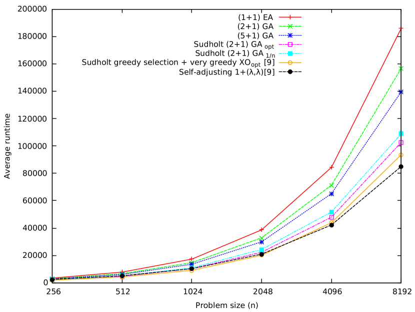
Figure 2: Average runtime over 1000 independent runs versus problem size $n$.

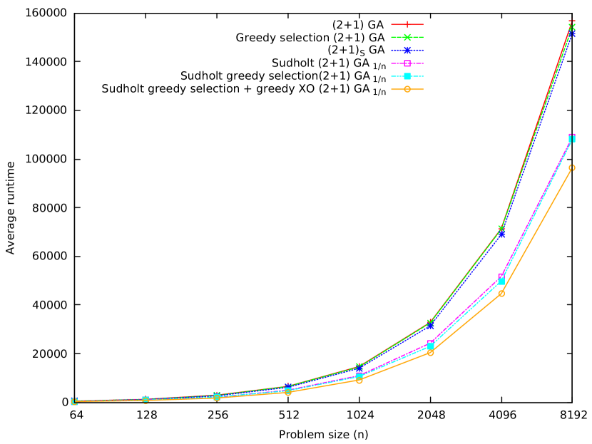
Figure 3: Comparison between standard selection, greedy selection and greedy selection + greedy crossover GAs. The runtime is averaged over 1000 independent runs.

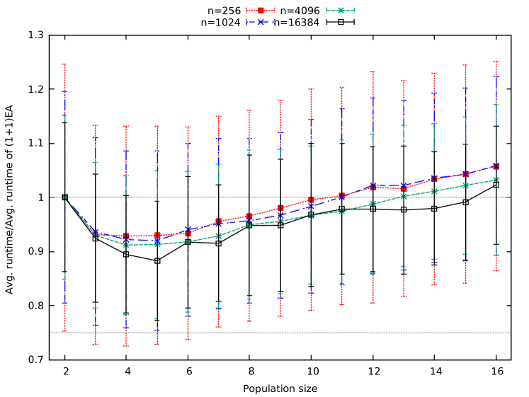
Figure 4: Average runtime gain of the ($\mu$+1) GA versus the (2+1) GA for different population sizes, errorbars show the standard deviation normalised by the average runtime for $\mu=2$.

The theoretical results presented in the previous sections pose some new interesting questions. On one hand, the theory suggests that population sizes greater than 2 benefit the ($\mu$+1) GA for hillclimbing the OneMax function. On the other hand, the best runtime bounds are obtained for a mutation rate of approximately $1.3/n$, suggesting that higher mutation rates than the standard $1/n$ rate may improve the performance of the ($\mu$+1) GA. In this section we present the outcome of some experimental investigations to shed further light on these questions. In particular, we will investigate the effects of the population size and mutation rate on the runtime of the steady-state GA for OneMax and compare its runtime against other GAs that have been proved to be faster than mutation-only EAs in the literature.

We start with an overview of the performance of the algorithms. In Fig. 2, we plot the average runtime over 1000 independent runs of the ($\mu$+1) GA with $\mu=2$ and $\mu=5$ (with uniform parent selection and standard $1/n$ mutation rate) for exponentially increasing problem sizes and compare it against the fastest standard bit mutation-only EA with static mutation rate (i.e., the (1+1) EA with $1/n$ mutation rate). While the algorithm using $\mu=5$ outperforms the $\mu=2$ version, they are both faster than the (1+1) EA already for small problem sizes. We also compare the algorithms against the (2+1) GA investigated by Sudholt [13] where diversity is enforced by the environmental selection always preferring distinct individuals of equal fitness - the same GA variant that was first proposed and analysed in [7]. We run the algorithm both with standard mutation rate $1/n$ and with the optimal mutation rate $(1+\sqrt{5})/(2n)$. Obviously, when diversity is enforced, the algorithms are faster. Finally, we also compare the algorithms against the (1+($\lambda$,$\lambda$)) GA with self-adjusting population sizes and Sudholt’s (2+1) GA as they were compared previously in [34]. Note that in [34] (Fig. 8 therein) Sudholt’s algorithm was implemented with a very greedy parent selection operator that always prefers distinct individuals on the highest fitness level for reproduction.

In order to decompose the effects of the greedy parent selection, greedy crossover and the use of diversity, we conducted further experiments shown in Figure 3. Here, we see that it is indeed the enforced diversity that creates the fundamental performance difference. Moreover, the results show that the greedy selection/greedy crossover GA is slightly faster than the greedy parent selection GA and that greedy parent selection is slightly faster than standard selection. Overall, the figure suggests that the lower bound presented in Theorem 12 is also valid for the standard (2+1) GA with uniform parent selection (i.e., no greediness). In Figure 3, it can be noted that the performance difference between the GA with greedy crossover and greedy parent selection analysed in [13] and the (2+1) GA with enforced diversity and without greedy crossover is more pronounced than the performance difference between the standard (2+1) GA analysed in Section 5 and the $(2+1)_{S}$ GA which was analysed in Section 6. The reason behind the difference in discrepancies is that the $(2+1)_{S}$ GA does not implement the greedy crossover operator when the Hamming distance is 2. We speculate that cases where the Hamming distance is just enough for the crossover to exploit it occur much more frequently than the cases where a larger Hamming distance is present. As a result, the performance of the $(2+1)_{S}$ GA does not deviate much from the standard algorithm. Table 1 presents the mean and standard deviation of the runtimes of the algorithms depicted in Figure 2 and Figure 3 over 1000 independent runs.

Now we investigate the effects of the population size on the ($\mu$+1) GA. We perform 1000 independent runs of the ($\mu$+1) GA with uniform parent selection and standard mutation rate $1/n$ for increasing population sizes up to $\mu=16$. In Fig. 4 we present average runtimes divided by the runtime of the $(2+1)$ GA and in Fig. 5 normalised against the runtime of the (1+1) EA. In both figures, we see that the runtime improves for $\mu$ larger than $2$ and after reaching its lowest value increases again with the population size. It is not clear whether there is a constant optimal static value for $\mu$ around 4 or 5. The experiments, however, do not rule out the possibility that the optimal static population size increases slowly with the problem size (i.e., $\mu=3$ for $n=256$, $\mu=4$ for $n=4096$ and $\mu=5$ for $n=16384$). On the other hand, we clearly see that as the problem size increases we get a larger improvement on the runtime. This indicates that the harder is the problem, more useful are the populations. In particular, in Figure 5 we see that the theoretical asymptotic gain of 25% with respect to the runtime of the (1+1) EA is approached more and more closely as $n$ increases. For the considered problem sizes, the ($\mu$+1) GA is faster than the (1+1) EA for all tested values of $\mu$. However, to see the runtime improvement of the ($\mu$+1) GA against the (2+1) GA for $\mu>15$ the experiments (Fig. 4) suggest that greater problem sizes would need to be used.

Finally, we investigate the effect of the mutation rate on the runtime. Based on our previous experiments we set the population size to the best seen value of $\mu=5$ and perform 1000 independent runs for each $c$ value ranging from $0.9$ to $1.9$. In Figure 6, we see that even though the mutation rate $c\approx 1.3$ minimises the upper bound we proved on the runtime, setting a larger mutation rate of $1.6$ further decreases the runtime.

Table 1: Statistics for the experimental results of Fig. 2 and Fig. 3

Algorithms	$n=64$		$n=128$		$n=256$		$n=512$
	Mean	Std. dev.	Mean	Std. dev.	Mean	Std. dev.	Mean	Std. dev.
(1+1) EA	612.66	208.88	1456.81	450.51	3397.72	887.07	7804.65	1791.44
(2+1) GA	546.57	179.61	1271.30	357.41	2952.70	727.84	6586.60	1378.50
Greedy (2+1) GA	519.93	177.28	1228.86	355.23	2854.18	730.07	6548.51	1434.21
(5+1) GA	529.29	156.19	1194.50	281.92	2744.80	595.41	6087.60	1164.30
Sudholt‘s (2+1) GA1/n	449.92	121.87	1040.26	277.71	2099.24	375.74	5022.30	873.47
Sudholt‘s (2+1) GAopt	427.87	108.51	978.50	212.13	2142.82	411.30	4682.88	742.95
(2+1)S GA	484.40	174.87	1183.80	366.28	2705.09	710.85	6183.55	1451.07
Sudholt’s greedy selection + greedy XO (2+1) GA1/n	326.21	108.04	790.47	223.50	1787.49	425.70	4105.20	851.14
Sudholt‘s greedy selection (2+1) GA1/n	410.56	117.45	958.64	222.26	2192.50	469.57	4801.66	901.88
Sudholt’s (2+1)GA diverse crossoveropt	386.14	104.59	907.719	222.24	1873.37	409.68	4243.65	812.38
Self-adjusting $1+(\lambda,\lambda)$	583.91	146.58	1209.14	164.96	2478.51	294.53	5084.68	462.34

Algorithms	$n=1024$		$n=2048$		$n=4096$		$n=8192$
	Mean	Std. dev.	Mean	Std. dev.	Mean	Std. dev.	Mean	Std. dev.
(1+1) EA	17267.39	3653.38	38636.71	6966.43	84286.18	13563.25	186012.84	28660.69
(2+1) GA	14715.00	2876.00	32843.00	5574.70	71346.00	10810.00	156800.00	23357.00
Greedy (2+1) GA	14553.66	2892.29	32667.89	6075.17	71149.61	11990.71	154354.66	23250.14
(5+1) GA	13538.00	2436.00	29907.00	4909.60	65136.00	9758.00	139590.00	18622.00
Sudholt‘s (2+1) GA1/n	10962.58	1960.08	24324.46	4543.38	51708.68	8772.04	108990.46	12729.60
Sudholt‘s (2+1) GAopt	10372.87	1545.92	22335.50	3117.32	47913.78	6094.81	102614.39	12261.37
(2+1)S GA	14028.86	2852.73	31403.85	5935.81	68957.18	11905.57	151635.40	25489.27
Sudholt’s greedy selection + greedy XO (2+1) GA1/n	9206.59	1713.77	20446.31	3691.36	44677.26	7311.26	96525.02	13997.87
Sudholt‘s greedy selection (2+1) GA1/n	10640.57	1777.29	23035.28	3624.30	49857.03	7123.71	108087.00	14881.14
Sudholt’s (2+1)GA diverse crossoveropt	9132.63	149.92	20098.44	3171.93	43815.65	6334.92	93581.99	12396.22
Self-adjusting $1+(\lambda,\lambda)$	10324.62	695.95	20951.38	1157.73	42216.53	1862.68	85028.97	2703.08

8 Conclusion

The question of whether genetic algorithms can hillclimb faster than mutation-only algorithms is a long standing one. On one hand, in his pioneering book, Rechenberg had given preliminary experimental evidence that crossover may speed up the runtime of population based EAs for generalised OneMax [35]. On the other hand, further experiments suggested that genetic algorithms were slower hillclimbers than the (1+1) EA [6, 21]. In recent years it has been rigorously shown that crossover and mutation can outperform algorithms using only mutation. Firstly, a new theory-driven GA called (1+($\lambda$,$\lambda$)) GA has been shown to be asymptotically faster for hillclimbing the OneMax function than any unbiased mutation-only EA [34]. Secondly, it has been shown how standard ($\mu$+$\lambda$) GAs are twice as fast as their standard bit mutation-only counterparts for OneMax as long as diversity is enforced through environmental selection [13].

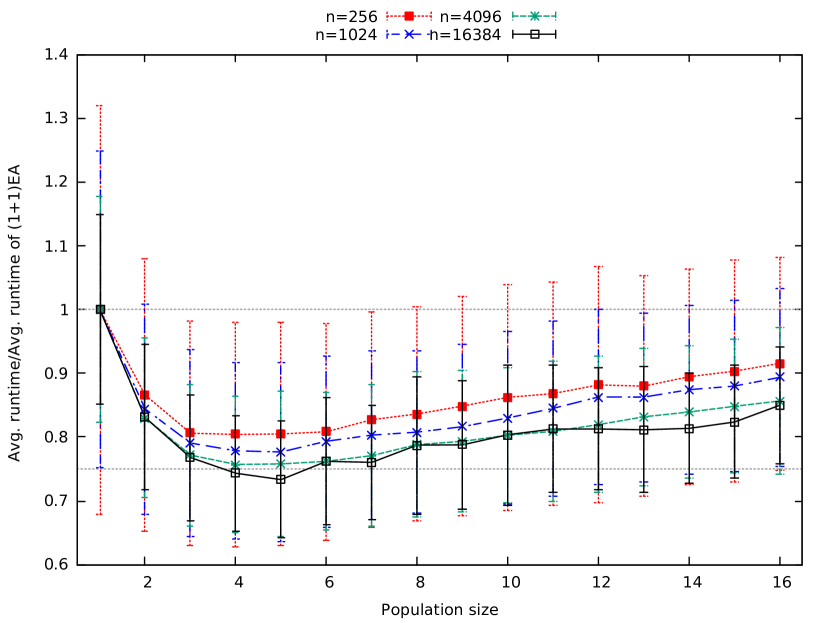
Figure 5: Average runtime gain of the ($\mu$+1) GA versus the (1+1) EA for different population sizes, errorbars show the standard deviation normalised by the average runtime of the (1+1) EA.

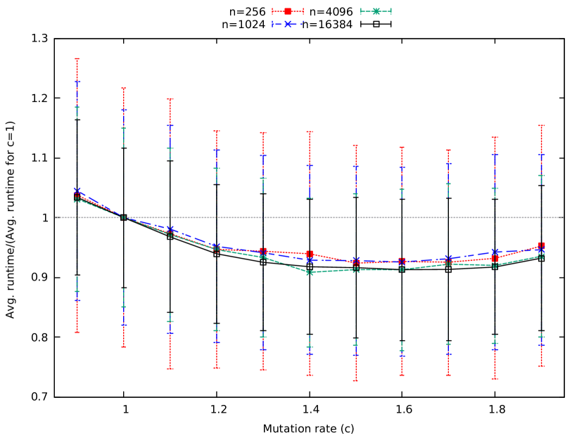
Figure 6: Average runtime gain of the (5+1) GA for various mutation rates versus the standard $1/n$ mutation rate, errorbars show the standard deviation normalised by the average runtime for $1/n$ mutation rate.

In this paper we have rigorously proven that standard steady-state GAs with $\mu\geq 3$ and $\mu=o(\log{n}/\log{\log{n}})$ are at least 25% faster than all unbiased standard bit mutation-based EAs with static mutation rate for OneMax even if no diversity is enforced. The Markov Chain framework we used to achieve the upper bounds on the runtimes should be general enough to allow future analyses of more complicated GAs, for instance with greater offspring population sizes or more sophisticated crossover operators. A limitation of the approach is that it applies to classes of problems that have plateaus of equal fitness. Hence, for functions where each genotype has a different fitness value our approach would not apply. An open question is whether the limitation is inherent to our framework or whether it is crossover that would not help steady-state EAs at all on such fitness landscapes.

Our results also explain that populations are useful not only in the exploration phase of the optimization, but also to improve exploitation during the hillclimbing phases. In particular, larger population sizes increase the probability of creating and maintaining diversity in the population. This diversity can then be exploited by the crossover operator. Recent results had already shown how the interplay between mutation and crossover may allow the emergence of diversity, which in turn allows to escape plateaus of local optima more efficiently compared to relying on mutation alone [16]. Our work sheds further light on the picture by showing that populations, crossover and mutation together, not only may escape optima more efficiently, but may be more effective also in the exploitation phase.

Another additional insight gained from the analysis is that the standard mutation rate $1/n$ may not be optimal for the ($\mu$+1) GA on OneMax. This result is also in line with, and nicely complements, other recent findings concerning steady state GAs. For escaping plateaus of local optima it has been recently shown that increasing the mutation rate above the standard $1/n$ rate leads to smaller upper bounds on escaping times [16]. However, when jumping large low-fitness valleys, mutation rates of about $2.6/n$ seem to be optimal static rates (see the experiment section in [36, 37]). For OneMax lower mutation rates seem to be optimal static rates, but still considerably larger than the standard $1/n$ rate.

New interesting questions for further work have spawned. Concerning population sizes an open problem is to rigorously prove whether the optimal size grows with the problem size and at what rate. Also determining the optimal mutation rate remains an open problem. While our theoretical analysis delivers the best upper bound on the runtime with a mutation rate of about 1.3/$n$, experiments suggest a larger optimal mutation rate. Interestingly, this experimental rate is very similar to the optimal mutation rate (i.e., approximately 1.618/$n$) of the ($\mu$+1) GA with enforced diversity proven in [13]. The benefits of higher than standard mutation rates in elitist algorithms is a topic that is gaining increasing interest [38, 39, 40].

Further improvements may be achieved by dynamically adapting the population size and mutation rate during the run. Advantages, in this sense, have been shown for the (1+($\lambda$,$\lambda$)) GA by adapting the population size [12] and for single individual algorithms by adapting the mutation rate [41, 42]. Generalising the results to larger classes of hillclimbing problems is intriguing. In particular, proving whether speed ups of the ($\mu$+1) GA compared to the (1+1) EA are also achieved for royal road functions would give a definitive answer to a long standing question [21]. Analyses for larger problem classes such as linear functions and classical combinatorial optimisation problems would lead to further insights. Yet another natural question is how the ($\mu$+1) GA hillclimbing capabilities compare to ($\mu$+$\lambda$) GAs and generational GAs.

References

- [1] D. E. Goldberg, Genetic Algorithms in Search, Optimization and Machine Learning. Addison-Wesley, 1989.
- [2] A. E. Eiben and J. E. Smith, Introduction to evolutionary computing. Springer, 2003.
- [3] T. Bäck, Evolutionary Algorithms in Theory and Practice. Oxford University Press, 1996.
- [4] J. H. Holland, Adaptation in Natural and Artificial Systems. University Michigan Press, 1975.
- [5] M. Mitchell, J. Holland, and S. Forrest, “Relative building-block fitness and the building block hypothesis,” in Foundations of Genetic Algorithms (FOGA ’93), vol. 2, 1993, pp. 109–126.
- [6] T. Jansen and I. Wegener, “Real royal road functions — where crossover provably is essential,” Discrete Applied Mathematics, vol. 149, no. 1-3, pp. 111–125, 2005.
- [7] ——, “The analysis of evolutionary algorithms-a proof that crossover really can help,” Algorithmica, vol. 34, no. 1, pp. 47–66, 2002.
- [8] D. Dang, T. Friedrich, T. Kötzing, M. S. Krejca, P. K. Lehre, P. S. Oliveto, D. Sudholt, and A. M. Sutton, “Escaping local optima with diversity mechanisms and crossover,” in Proceedings of the Genetic and Evolutionary Computation Conference (GECCO 2016). ACM, 2016, pp. 645–652.
- [9] B. Doerr and C. Doerr, “A tight runtime analysis of the (1+(, )) genetic algorithm on onemax,” in Proceedings of the Genetic and Evolutionary Computation Conference (GECCO 2015). ACM, 2015, pp. 1423–1430.
- [10] B. Doerr, C. Doerr, and F. Ebel, “From black-box complexity to designing new genetic algorithms,” Theoretical Computer Science, vol. 567, pp. 87 – 104, 2015.
- [11] P. K. Lehre and C. Witt, “Black-box search by unbiased variation,” Algorithmica, vol. 64, no. 4, pp. 623–642, 2012.
- [12] B. Doerr and C. Doerr, “Optimal parameter choices through self-adjustment: Applying the 1/5-th rule in discrete settings,” in Proceedings of the Genetic and Evolutionary Computation Conference (GECCO 2015). ACM, 2015, pp. 1335–1342.
- [13] D. Sudholt, “How crossover speeds up building-block assembly in genetic algorithms,” Evolutionary Computation, vol. 25, no. 2, pp. 237–274, 2017.
- [14] ——, “A new method for lower bounds on the running time of evolutionary algorithms,” IEEE Transactions on Evolutionary Computation, vol. 17, no. 3, pp. 418–435, 2013.
- [15] C. Witt, “Tight bounds on the optimization time of a randomized search heuristic on linear functions,” Combinatorics, Probability & Computing, vol. 22, no. 2, pp. 294–318, 2013.
- [16] D. Dang, T. Friedrich, T. Kötzing, M. S. Krejca, P. K. Lehre, P. S. Oliveto, D. Sudholt, and A. M. Sutton, “Emergence of diversity and its benefits for crossover in genetic algorithms,” in International Conference on Parallel Problem Solving from Nature (PPSN XIV), 2016, pp. 890–900.
- [17] J. Sarma and K. D. Jong, “Generation gap methods,” in Handbook of evolutionary computation, T. Back, D. B. Fogel, and Z. Michalewicz, Eds. IOP Publishing Ltd., 1997, ch. C 2.7.
- [18] J. E. Rowe, “Genetic algorithms,” in Handbook of computational Intelligence, W. Pedrycz and J. Kacprzyk, Eds. Springer, 2011, pp. 825–844.
- [19] T. Kötzing, D. Sudholt, and M. Theile, “How crossover helps in Pseudo-Boolean optimization,” in Proceedings of the Genetic and Evolutionary Computation Conference (GECCO 2011). ACM Press, 2011, pp. 989–996.
- [20] T. Storch and I. Wegener, “Real royal road functions for constant population size,” Theoretical Computer Science, vol. 320, no. 1, pp. 123–134, 2004.
- [21] M. Mitchell, J. Holland, and S. Forrest, “When will a genetic algorithm outperform hill climbing?” in Neural Information Processing Systems (NIPS 6). Morgan Kaufmann, 1994, pp. 51–58.
- [22] D. Sudholt, “Crossover is provably essential for the ising model on trees,” in Proceedings of the Genetic and Evolutionary Computation Conference (GECCO 2005). New York, New York, USA: ACM Press, 2005, pp. 1161–1167.
- [23] P. K. Lehre and X. Yao, “Crossover can be constructive when computing unique input–output sequences,” Soft Computing, vol. 15, no. 9, pp. 1675–1687, 2011.
- [24] B. Doerr, E. Happ, and C. Klein, “Crossover can provably be useful in evolutionary computation,” Theoretical Computer Science, vol. 425, pp. 17–33, 2012.
- [25] F. Neumann, P. S. Oliveto, G. Rudolph, and D. Sudholt, “On the effectiveness of crossover for migration in parallel evolutionary algorithms,” in Proceedings of the Genetic and Evolutionary Computation Conference (GECCO 2011). ACM Press, 2011, pp. 1587–1594.
- [26] C. Qian, Y. Yu, and Z. Zhou, “An analysis on recombination in multi-objective evolutionary optimization,” Artificial Intelligence, vol. 204, pp. 99 – 119, 2013.
- [27] B. Doerr and C. Winzen, “Playing mastermind with constant-size memory,” Theory of Computing Systems, vol. 55, no. 4, pp. 658–684, 2014.
- [28] B. Doerr, C. Doerr, R. Spöhel, and T. Henning, “Playing mastermind with many colors,” Journal of the ACM, vol. 63, no. 5, pp. 42:1–42:23, 2016.
- [29] B. Doerr, C. Doerr, and T. Kötzing, “The right mutation strength for multi-valued decision variables,” in Proceedings of the Genetic and Evolutionary Computation Conference (GECCO 2016). ACM, 2016, pp. 1115–1122.
- [30] T. Jansen, Analyzing evolutionary algorithms: The computer science perspective. Springer, 2013.
- [31] P. S. Oliveto and X. Yao, “Runtime analysis of evolutionary algorithms for discrete optimization,” in Theory of Randomized Search Heuristics: Foundations and Recent Developments, B. Doerr and A. Auger, Eds. World Scientific, 2011, pp. 21–52.
- [32] C. Witt, “Runtime analysis of the (+1) ea on simple pseudo-boolean functions,” Evolutionary Computation, vol. 14, no. 1, pp. 65–86, 2006.
- [33] T. Friedrich, P. S. Oliveto, D. Sudholt, and C. Witt, “Analysis of diversity-preserving mechanisms for global exploration,” Evolutionary Computation, vol. 17, no. 4, pp. 455–476, 2009.
- [34] B. Doerr, C. Doerr, and F. Ebel, “From black-box complexity to designing new genetic algorithms,” Theoretical Computer Science, vol. 567, pp. 87–104, 2015.
- [35] I. Rechenberg, Evolutionsstrategie: Optimierung technischer Systeme nach Prinzipien der biologishen Evolution. Friedrich Frommann Verlag, 1973.
- [36] D.-C. Dang, T. Friedrich, T. Kötzing, M. S. Krejca, P. K. Lehre, P. S. Oliveto, D. Sudholt, and A. M. Sutton, “Escaping Local Optima using Crossover with Emergent or Reinforced Diversity,” ArXiv, Aug. 2016.
- [37] ——, “Escaping local optima using crossover with emergent diversity,” IEEE Transactions on Evolutionary Computation, pp. –, 2017, in Press.
- [38] P. S. Oliveto, P. K. Lehre, and F. Neumann, “Theoretical analysis of rank-based mutation-combining exploration and exploitation,” in IEEE Congress on Evolutionary Computation (CEC 2009). ACM, 2017, pp. 1455–1462.
- [39] D. Corus, P. S. Oliveto, and D. Yazdani, “On the runtime analysis of the opt-ia artificial immune system,” in Proceedings of the Genetic and Evolutionary Computation Conference (GECCO 2017). ACM, 2017, pp. 83–90.
- [40] B. Doerr, H. P. Le, R. Makhmara, and T. D. Nguyen, “Fast genetic algorithms,” in Proceedings of the Genetic and Evolutionary Computation Conference (GECCO 2017). ACM, 2017, pp. 777–784.
- [41] B. Doerr, C. Doerr, and J. Yang, “k-bit mutation with self-adjusting k outperforms standard bit mutation,” in International Conference on Parallel Problem Solving from Nature (PPSN XIV). Springer, 2016, pp. 824–834.
- [42] A. Lissovoi, P. S. Oliveto, and J. A. Warwicker, “On the runtime analysis of generalised selection hyper-heuristics for pseudo-boolean optimisation,” in Proceedings of the Genetic and Evolutionary Computation Conference (GECCO 2017). ACM, 2017, pp. 849–856.