Multiphase Aluminum A356 Foam Formation Process Simulation Using Lattice Boltzmann Method

Abstract

Shan-Chen model is a numerical scheme to simulate multiphase fluid flows using Lattice Boltzmann approach. The original Shan-Chen model suffers from inability to accurately predict behavior of air bubbles interacting in a non-aqueous fluid. In the present study, we extended the Shan-Chen model to take the effect of the attraction-repulsion barriers among bubbles in to account. The proposed model corrects the interaction and coalescence criterion of the original Shan-Chen scheme in order to have a more accurate simulation of bubbles morphology in a metal foam. The model is based on forming a thin film (narrow channel) between merging bubbles during growth. Rupturing of the film occurs when an oscillation in velocity and pressure arises inside the channel followed by merging of the bubbles. Comparing numerical results obtained from proposed model with mettallorgraphy images for aluminum A356 demonstrated a good consistency in mean bubble size and bubbles distribution.

1 Introduction

Demanding for advanced materials are increasing rapidly via new technologies. Closed cell metal foams gained a lot of interest as one of the major branches of advanced materials due to their unique physical and mechanical properties, including high specific strength and compressibility along with good energy absorption capability [1, 2, 3, 4].

Despite the advantages, the employment of metal foams in industrial applications is limited due to the inhomogeneity of the structure which results in the deviation of the mechanical properties of the foams from what predicted by the scaling relations. This is mainly due to the morphological defects such as missing or wavy distortions of the cell walls and non-uniform shape and size of the cells which results in poor reproducibility of foam structures [5]. In metals, unlike ionic liquids, the formation mechanisms of metal foam has not yet fully understood [5].

Bubble stability is the primitive challenge in understanding the mechanism of metal foam formation. A variety of studies and researches have been performed by scientists in order to investigate and analyze the parameters affecting bubble stabilization [4, 5, 6, 7, 8, 9, 10, 11, 12, 13, 14]. Most of the investigations have focused on formation of single bubble in ionic liquid environment, especially water, with no impurity [8, 10, 11, 12, 13, 14]. However, even in the purest condition, molten metal contains dozens of different impurities. Another important issue which has been neglected during various studies is the multi-bubble nature of metal foam formation process, which mostly appears in bubbles interactions. In addition, due to the presence of metallic bond in metal melt, there is no ionic or polar attraction and repulsion forces, which causes a different behavior of the liquid-gas interface in metal melts in comparison with aqueous solutions [4, 5, 6, 7].

In order to have a computational study on metal foam formation process, a basic understanding of bubble stability conditions in the presence of particles is required. Therefore, a computational model based on known dynamics of bubbles and improving it using the computational-experimental approach has to be built, which is accomplished by adding some constraints that are focused on the boundary of each bubble according to available theories and verify the selected ones using an experiment [5].

Most of the studies in the field of bubble dynamics investigated single bubble dynamics in aqueous solutions or water based liquids and only a few are conducted to study multi bubble dynamics and foam formation process.

Chine and Monno [9] developed an axial symmetry model to simulate the behavior of a single gas bubble expansion, embedded in a viscous fluid using Finite Element Method. Ghosh and Das [15] conducted a numerical investigation of single bubble dynamics using Lattice Boltzmann Method. Their model contains a rising gas bubble inside a tube filled with liquid. They validated and verified different aspects of using Lattice Boltzmann Method in simulating trapped gas bubbles in liquids .

Chahine [10] studied the dynamics of clouds of bubbles via both analytical technique and numerical simulation using 3D Boundary Element Method (BEM). They also studied the behavior of bubbles in a non-uniform flow field and their response to flow. Chahine [11] investigated influence flow field to interaction of bubbles. Ida [12] conducted a mathematical modeling using a nonlinear multi-bubble model from pressure pulses perspective. Bermond et al. [13] performed an outstanding computational investigation on bubble interactions and validated it using a novel experimental procedure. The dynamics of bubbles in that research was studied based on Rayleigh-Plesset equation. Kim et al. presented an Immersed Boundary Method (IBM) to simulate and predict the 2D structure of a dry foam. This method allows one to study pressure equilibrium in non-conventional approach. In their model, a set of thin boundaries partition the gas into discrete cells or bubbles [16].

The Lattice Boltzmann (LB) simulation has been used extensively to simulate the kinetic effects on bubbles [17]. Advantage of LB approach lies in the fact that there are no global systems of equations which have to be solved. Besides, boundaries in simulation domain do not have an effective impact on the computation time. These features are essential for foam formation simulation regarding the complex internal structure of foams. Andrel et al. [18] used Lattice Boltzmann to simulate flow in a simplified single phase model as an alternative to a liquid-gas two phase model to analyze bubble interaction in protein foams in order to determine bubble coalescence conditions. Leung et al. [19] studied bubbles nucleation, growth, stability conditions and interaction in plastic foaming process.

Beugre et al. [20] developed a 3D Lattice Boltzmann code to simulate fluid flow in metal foam. Pressure drop was the criteria used to compare the obtained results with experimental measurements. Computer aided X-ray microtomography was used to produce the 3D geometry of metal foam imported in LB simulation. They improved the computed geometry of the metal foam later with more advanced techniques in order to obtain better results .

Körner [5] conducted a thorough research using Lattice Boltzmann method to simulate the growth and formation of an aluminum metal foam using a single phase model. Diop et al. simulated solidification process of metal foams using Lattice Boltzmann Method [21]. Their numerical model included aluminum melt with gassing agent heated to obtain metallic foam.

In this study we constructed a hybrid experimental-computational model to predict the structure of a two-dimensional closed-cell aluminum foam. Most of the simulations conducted in this field are based on single phase models, while a two-phase computational model is adopted in the present study. To this end, a modified and improved Shan-Chen model is developed for multiphase simulations. Besides, a novel boundary condition is utilized to simulate oxide network particles’ effect on the interaction of two bubbles. This method can be extended to account for a larger number of bubbles in order to simulate metallic foams. The proposed model is created based on an experimental procedure and actual samples’ structures. Moreover, some additional phenomena such as random nucleation, growth, coalescence, and aging of bubbles are also developed in this model.

2 Mathematical Modeling

It is assumed that there is no variation in liquid temperature during foaming process, and the fluid flow is considered to be incompressible. Consequently, conservation of mass and momentum in a single phase continuum can be written as follows [22]:

$$\nabla.\textbf{u}=0$$ (1)

$$\frac{\partial\textbf{u}}{\partial t}+\left(\nabla.\textbf{u}\right)\textbf{u}=-\frac{1}{\rho}\nabla p+\nu\nabla^{2}\textbf{u}+g$$ (2)

where $t$, $u$, $p$, $\rho$, $\nu$, $g$ are time, velocity, pressure, density, kinematic viscosity and gravity, respectively.

In addition to conservation equations, gas pressure ($P_{i}$) in bubble ($i$) could be expressed by ideal gas equation [8]:

$${p_{i}}=\frac{{{n_{i}}.R.T}}{{{V_{i}}}}$$ (3)

where $R$ is gas constant, $n_{i}$ gas mole, $T$ temperature and $V_{i}$ is volume of bubble $i$. Gas and liquid were coupled at the interface by momentum balance and controlled by $\Gamma$ parameter. For having a stable bubble, velocity of fluid and gas must be equal at the interface.

$${v_{G}}(x)={v_{F}}(x)\qquad\forall\,x\in\Gamma$$ (4)

In order to estimate the pressure during the growth or expansion of the bubble, the kinetics of expansion of a single bubble of radius $R$ in an incompressible fluid with viscosity of $\rho$ and pressure $p_{0}$ is considered as basic calculations and due to the symmetry of the problem, the NSE equation can be reduced to Rayleigh equation[8] in spherical coordinates. Thus the bubble growth with radius $R$ can be calculated from Eq. 5.

$$\rho R\mathop{R}\limits^{..}+\frac{3}{2}\rho\mathop{{R^{2}}}\limits^{.}\quad+4\rho\nu\frac{{\mathop{R}\limits^{.}}}{R}\quad+\frac{{2\sigma}}{R}={p_{i}}-{p_{0}}$$ (5)

where $\mathop{R}\limits^{.}$ is $\frac{\partial R}{\partial t}$ and $\mathop{R}\limits^{..}$ is $\frac{\partial^{2}R}{\partial t^{2}}$. Each of the four terms of the Eq. 5 from left to right represents the excess bubble pressure, capillary pressure, viscous pressure and inertia pressure where $p_{i}$ denotes the bubble pressure and $\sigma$ is the surface tension. The Rayleigh equation expresses equilibrium between inertia, viscous and capillary forces, which prevent bubble expansion. However, in practice these forces will play a major role that is unclear and entirely depends on foam material and process parameters [4].

In this study it is assumed that blowing agent with specified weight percent was added to molten metal, uniformly distributed and dissolved by stirring. Then micro bubbles were abruptly produced by dissolution reaction of blowing agent in throughout the domain.

Nucleation occurs in random points in the domain. After nucleation, bubble growth will begin. For growth modeling in each time step, gas will be added by virtual blowing agent (proportional to blowing agent weight and gas production rate) in each bubble, and then the bubble volume will be increased due to the pressure balance. Gas blowing or growth will continue until all virtual blowing agent gases are added to the domain. Other phenomena, such as drainage and wall rupture are considered in growth process by bubble equilibrium equations. Condition of wall rupture could be added as an experimental or a mathematical criterion. One would consider this condition experimentally. For example, if the cell wall thickness falls below a critical thickness (which is a material characteristic), cell wall rupture will occur. This critical number for aluminum melt is reported as $50\mu m$, determined by X-ray radiography [6]. In this study, a computational criterion will be obtained from second derivative of pressure ($\triangledown^{2}p$).

Hydrodynamics, gas release and diffusion are necessary for the foaming stage. The blowing gas solubility in the fluid is finite. The gas concentration in the fluid can be calculated by the diffusion equation:

$${\partial_{t}}c+{\upsilon_{x}}{\partial_{x}}c-{\partial_{x}}(D{\partial_{x}}c))=Q$$ (6)

where $c=c(x,t)$ is concentration field of dissolved gas, $D$ gas diffusion constant and $Q=Q(x,t)$ is source term. The source term ($Q$) describes the blowing agent decomposition. There are two key points which have to be considered. One is gas solubility and the other is gas diffusion distance. In this study the concentration of dissolved hydrogen in molten and solid aluminum (C) is calculated from Eq. 7 and Eq. 8 respectively [4]:

$$C=5.84\frac{{c{m^{3}}}}{g}.\exp(-\frac{{6357K}}{T})\sqrt{\frac{p}{{bar}}}\qquad\small\text{For melt }$$ (7)

$$C=0.25\frac{{c{m^{3}}}}{g}.\exp(-\frac{{5941K}}{T})\sqrt{\frac{p}{{bar}}}\qquad\small\text{For solid}$$ (8)

Diffusion distance $\delta^{dif}$ is calculated from Eq. 9 where $D$ denotes the diffusion coefficient and $t$ the characteristic time [4]:

$${\delta^{dif}}=\sqrt{4Dt}$$ (9)

The diffusion length is a measure for the region of influence of a blowing agent particle. For example, if $\delta^{dif}$ is significantly larger than the mean particle distance, then a strong mutual influence has to be expected. The diffusion length is a measure for the region of influence of a blowing agent particle.

In this study, diffusion coefficient of hydrogen in aluminum is calculated from Eq. 10 [4]:

$$D={D_{0}}.\exp(-\frac{H}{{RT}})=\left\{{\begin{array}[]{*{20}{c}}{3.8.{{10}^{-6}}\frac{{{m^{2}}}}{s}.\exp(-\frac{{19.26kJ/mol}}{{RT}})}\\ {1.1.{{10}^{-5}}\frac{{{m^{2}}}}{s}.\exp(-\frac{{40.95kJ/mol}}{{RT}})}\end{array}}\right.$$ (10)

where $D_{0}$ is a constant, $R$ is the gas constant, $T$ is the temperature and $H$ the activation enthalpy. From Eq. 10, the diffusion coefficient at 700 ${}^{\circ}C$ is $D_{700^{\circ}C}=3.51\times 10^{-7}\frac{m^{2}}{s}$ and diffusion length of hydrogen is $374\mu m$. This length is small compared to the overall dimension of casting. Thus, gas concentration uniformity cannot be expected. Consequently, inhomogeneous distribution of blowing agent in melt will lead to non-uniform porosity. Experimental observations have confirmed this theory [4].

2.1 Numerical Model

2.1.1 Lattice Boltzmann approach

The LB method has shown to be suitable for foam formation problems [23]. Random micro bubbles in a virtual medium nucleate and interact within a set of rules. If correct physics is applied in the simulation, spontaneous hydrodynamic behavior can be expected. It can be said that LB method is a mesoscopic approach that is between macroscopic CFD approaches and microscopic molecular dynamics. Many multiphase models exist that use the LB method, such as Immiscible Lattice Boltzmann (ILBM) [24] Shan-Chen Model [25, 26], Free energy model [27, 28], Chromodynamic model [29] and HSD model [30].

LB method models fluid dynamics by evaluating particle distribution function $f(x,v,t)$ at each lattice point, where $f$ is the probability of finding a moving fluid particle with velocity $v$ at point $x$ and time $t$. By knowing $f$, one could get the values of density and momentum. The distribution function used in LB method, $f_{i}$, is a discretized form of the main continues function. Discretization means dividing the space into a finite number of lattices in order to present different parameters on these points, e.g. velocities could be evaluated by displacement vectors as ($\delta t.\textbf{e}_{i}$) where ($\delta t$) is time step and $i$ is displacement direction.

At each lattice point, different sets of distribution function would be defined. Two mostly used functions are $f$ and $h$. The $f$ function models mass and momentum transports and the $h$ function perform energy transport modeling. The macroscopic parameters are given by aggregating these distribution functions [31]:

$$\rho=\sum_{i}f_{i},\quad\rho\textbf{u}=\sum_{i}\textbf{e}_{i}f_{i},\quad E=\sum_{i}h_{i}$$ (11)

where $\rho$ is the density, u the macroscopic velocity and $E$ the energy density. As we have neglected thermal perturbation and solidification of liquid phase in present study, the energy transportations and its related functions will not be discussed further here.

The displacement of distributions is summarized by the equations of motion [32]:

$$f_{i}\left(\textbf{x}+e_{i},t+\Delta t\right)-f_{i}\left(\textbf{x},t\right)=\frac{\Delta t}{\tau_{f}}\left(f_{i}^{eq}\left(\textbf{x},t\right)\right)+F_{i}$$ (12)

where $f_{i}(\textbf{x},t)$ is the density distribution function in i direction. In order to model external forces such as gravity, one would use [32]:

$$F_{i}=W_{i}\rho\left[\frac{\left(\textbf{e}_{i}-\textbf{u}\right)}{c_{s}^{2}}+\frac{\left(\textbf{e}_{i}\cdot\textbf{u}\right)}{c_{s}^{2}}\right]\cdot\textbf{g}$$ (13)

$f^{eq}_{i}(\textbf{x},t)$ is equilibrium distribution function [32]:

$$f_{i}^{eq}\left(\textbf{x},t\right)=w_{i}\rho\left[1+\frac{\left(\textbf{e}_{\textbf{i}}\cdot\textbf{u}\right)}{c_{s}^{2}}+\frac{\left(\textbf{e}_{\textbf{i}}\cdot\textbf{u}\right)^{2}}{2c_{s}^{4}}-\frac{\textbf{u}^{2}}{2c_{s}^{2}}\right]$$ (14)

For a two dimensional D2Q9 model (2D with 9 velocity directions), the velocity direction $\textbf{e}_{i}$ and the weight $\omega_{i}$ are given by [32]:

$$\textbf{e}_{i}=\left\{\begin{array}[]{l l}\left(0,0\right),&\quad i=0\\ \left(\pm c,0\right),\left(0,\pm c\right)&\quad i=1,\cdots,4\\ \left(\pm c,\pm c\right)&\quad i=5,\cdots,8\\ \end{array}\right.$$ (15)

$$w_{i}=\left\{\begin{array}[]{l l}4/9,&\quad i=0\\ 1/9&\quad i=1,\cdots,4\\ 1/36&\quad i=5,\cdots,8\\ \end{array}\right.$$ (16)

The viscosity $\nu$ is given by:

$$\nu=c_{s}^{2}\Delta t\left(\tau_{f}-0.5\right)$$ (17)

where $\tau_{f}$ is the relaxation time for velocity field in dimensionless form.

Equation of motion (Eq. 12) is solved by LBM in two steps, as noted earlier, known as collision and streaming [32]:

Collision:

$$f_{i}^{out}\left(\textbf{x},t\right)=f_{i}^{in}\left(\textbf{x},t\right)+\frac{\Delta t}{\tau_{f}}\left(f_{i}^{eq}\left(\textbf{x},t\right)-f_{i}^{in}\left(\textbf{x},t\right)\right)+F_{i}$$ (18)

Streaming:

$$f_{i}^{in}\left(\textbf{x}+e_{i},t+\Delta t\right)=f_{i}^{out}\left(\textbf{x},t\right)$$ (19)

where $f^{out}_{i}$ and $f^{in}_{i}$ are outgoing (after collision) and incoming (before collision) distribution functions respectively.

2.1.2 Shan-Chen model

Shan-Chen model is based on incorporating long-range attractive forces (F) between distribution functions. In the original Shan-Chen model, the interacting force is approximated using the following equation [25, 26]:

$$F\left(x\right)\cong-\frac{d^{2}b}{D}\psi\left(x\right)g\bigtriangledown\psi\left(x\right)$$ (20)

Where $b$ is the number of nearest sites with equal distance, $D$ is the dimension of the space and $g$ is proportional to the interaction strength. The function $\psi$ is so-called pseudopotential and is a function of time and location. Other adjacent sites (next nearest) can be considered in the Eq. 20 which leads to a more general form of the above equation [33]:

$$F\left(x\right)=-c_{0}\psi\left(x\right)g\bigtriangledown\psi\left(x\right)$$ (21)

In the Shan-Chen model the force at a given lattice point depends on all local neighbor’s characteristics. So the following can be written:

$$F_{\alpha}\left(x\right)=-G\psi\left(x\right)\Sigma_{i}w_{i}\psi\left(x+e_{i}\right)e_{i}$$ (22)

where coefficient $G$ controls the strength of the attraction. The function $\psi$ is $\psi=\psi\left(x\right)$, where $\rho$ depends on time and location. $c_{i}$ and $w_{i}$ are respectively lattice velocity vector and its weight in selected lattice model. Therefore, force is introduced to account for attraction. The contributions of state and surface tension to the equation can be observed through Taylor expansion. Taylor expansion of the force can be written as [34]:

$$F_{\alpha}\left((x)\right)=-G\psi\left(x\right)\left(\frac{1}{3}\partial_{\alpha}\psi+\frac{1}{18}\partial_{\alpha}\Delta\psi\right)+O\left(\partial^{5}\right)$$ (23)

The following formulation is derived algebraically [34]:

$$F_{\alpha}\left((x)\right) =-G\psi\left(x\right)\left(\frac{1}{3}\partial_{\alpha}\psi+\frac{1}{18}\partial_{\alpha}\Delta\psi\right)$$

$$=-G\left(\frac{1}{6}\partial_{\alpha}\psi^{2}+\frac{1}{18}\left(\partial_{\alpha}\left(\psi\Delta\psi\right)-\Delta\psi\partial_{\alpha}\psi\right)\right)$$

$$=-G\left(\frac{1}{6}\partial_{\alpha}\psi^{2}+\frac{1}{18}\left(\partial_{\alpha}\left(\psi\Delta\psi\right)+\frac{1}{2}\partial_{\alpha}|\bigtriangledown\psi|^{2}\right.\right.$$

$$\quad-\partial_{\beta}\partial_{\alpha}\psi\partial_{\beta}\psi\bigg{)}\bigg{)}$$ (24)

The force influence can be included to in the momentum-flux tensor [34, 33]:

$$\partial_{\beta}P_{\alpha\beta}=-F_{\alpha}+\partial_{\alpha}p$$ (25)

The equation of state for the LBE is $p=c^{2}_{s}\rho$ so:

$$\partial_{\beta}P_{\alpha\beta}=-F_{\alpha}+\partial_{\alpha}\left(c^{2}_{s}\rho\right)$$ (26)

Thus, the flux tensor $P_{\alpha\beta}$ is modified as follows:

$$P_{\alpha\beta}=\left(c^{2}_{s}\rho+\frac{G}{6}\psi^{2}+\frac{G}{36}|\bigtriangledown\psi|^{2}+\frac{G}{18}\psi\bigtriangleup\psi\right)\delta_{\alpha\beta}$$

$$-\frac{G}{18}\partial_{\alpha}\psi\partial_{\beta}\psi$$ (27)

By analogy with classical mechanics, the potential of the force can be introduced as:

$$U=\frac{G}{6}\psi^{2}+\frac{G}{36}|\bigtriangledown\psi|^{2}+\frac{G}{18}\psi\bigtriangleup\psi$$ (28)

Since the gradient terms in Eq. 28 are in small compared to the leading terms (the characteristic length of the interface is longer than the lattice spacing, as in all diffuse-interface methods), the Eq. 28 can be approximated:

$$p=\rho c^{2}_{s}+\frac{G}{6}\psi^{2}$$ (29)

By a suitable choice of the pseudo-potential $\psi\left(x\right)$, this equation can describe the separation of phases. One simple and usual choice can be $\psi=\rho$. By using this pseudo-potential function, the momentum flux tensor resembles diffuse interface method. However, the choice of $\psi=\rho\left(x,t\right)$ is not the best in terms of stability. When $\psi$ equals $\rho$, it becomes larger for larger $\rho$. Thus, the attractive potential contains a malfunctioning loop: the larger density $\rho$ leads to a larger $\psi$ which causes larger gradients and instabilities. $\psi=\rho$ is good for small gas-liquid density ratios.

In the case of aluminum liquid and hydrogen gas (two-phase system), density ratio is considerably higher. Therefore, to handle the pseudopotential function $\psi$ for larger $\rho$ while preserving its ratio for smaller $\rho$, the following choice of the pseudopotential is used:

$$\psi\left(\rho\right)=1-exp\left(-\rho\right)$$ (30)

Which is for small $\rho$ equals to $\psi\left(x\right)=\rho$ (Fig.1) and for large densities, $\psi\left(x\right)=1$ (Fig.2). This choice of the pseudopotential allows separation of gas and liquid in larger density ratios (if not more than 60-70) [35].

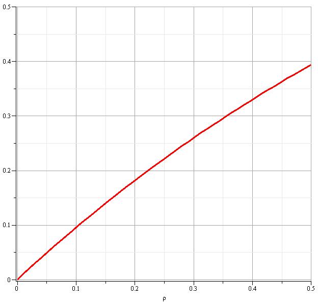
Figure 1: Pseudopotential function, zoomed to show its linearity for small densities

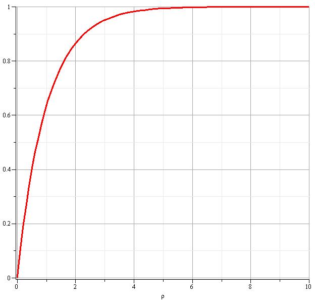
Figure 2: Pseudopotential function, which yields 1 as approaches infinity (large densities)

The critical value, when separation occurs, can be calculated from the thermodynamic theory by these two equations [36]:

$$\frac{dp_{0}}{d\rho}=0$$ (31)

$$\frac{d^{2}p_{0}}{d\rho^{2}}=0$$ (32)

By substituting Eq. 30 in Eq. 29 and for D2Q9 lattice ($c_{s}=\frac{1}{\sqrt{3}}$):

$$p_{0}=\frac{\rho}{3}+\frac{G}{6}\left(1-exp\left(-\rho\right)\right)$$ (33)

And from Eq. 31 and Eq. 32 one would get:

$$\frac{1}{3}+\frac{G_{critical}}{3}exp\left(-\rho_{critical}\right)\left(1-exp\left(-\rho_{critical}\right)\right)=0$$

$$-\frac{G_{critical}}{3}exp\left(-\rho_{critical}\right)\left(1-exp\left(-\rho_{critical}\right)\right)$$

$$\qquad+\frac{G_{critical}}{3}exp\left(-2\rho_{critical}\right)=0$$ (34)

Solving these equations lead to $G_{critical}=-4$ and $\rho_{critical}=ln2$. This means that if the system is initialized with the liquid density more than ln 2 and the gas density less than ln 2 in simulations with $G\leq-4$, the result is stable and separation will occur.

2.1.3 Bubble nucleation and growth

Number of bubble nucleation sites depends on the initial amount and size of the blowing agents. This number which is based on experimental results, is initially inserted into the main procedure. A time random subroutine is used to determine nucleation site positions in a 2D domain. These locations called “domain gas points” are in fact virtual blowing agents which in lattice domain are defined as gas nuclei and hydrogen density resulting from decomposition of the blowing agents, is accordingly calculated for these points. Other lattice points are set as liquid and give aluminum density. After this step, all numbers and parameter are changed to dimensionless parameters by open source OpenLB code [37]. Hydrogen gas release rate is calculated in each time step and added to each lattice point by pressure increment.

$$\frac{dp}{dt}=A\times\frac{\frac{dn}{dt}}{N}$$ (35)

where $\frac{dp}{dt}$ is pressure increase rate for each lattice point that refers to gas, $A$ is a constant which depends on gas behavior (in case of ideal gas $A=\frac{RT}{V}$ where $R$ is gas constant, $T$ temperature and $V$ is volume), $\frac{dn}{dt}$ is gas release rate in $\frac{mole}{sec}$ and $N$ is population of lattice gas points. Thus, because of pressure increase, pressure expansion is defined by multiphase code that has been developed in this work.

2.1.4 Program algorithm

The flowchart of the main program algorithm is shown in Fig. 3. Present code has been developed base on OpenLB open source code. The Shan-Chen model was incorporated and some modifications were added to the core structure of this algorithm. . In Fig. 3, the red boxes are the codes developed by open source community and the green boxes demonstrate the developed or modified parts, which where achieved in this study.

Figure 3: Main Program Algorithm (Green: User Codes, Red: Open Source Codes)

2.1.5 Bubbles interaction and modification of Shan-Chen model

Interaction of bubbles in pure liquid, without suspended solid, modeling techniques is completely different from liquids containing floating particles (e.g. SiC particles in molten aluminum). In case of two moving bubbles in pure aqueous liquid, if they are closed to each other, common behavior is increment in their surface curvature, that leads to merging and coalescence phenomena from the contact tip (See Fig. 4). However, as shown in Fig. 5 for molten metals, due to existence of a lot of solid particles (impurities and inclusions), interaction between bubbles have a different behavior. Experimental observations during aluminum foam production show a particles network see Fig. 5 between bubbles, which is often called oxide network [7]. This network at interface act as a mechanical barrier and prevent further cell wall thinning. Therefore, main mechanism of foam stabilization between bubbles is due to particle confinement (See Fig. 5).

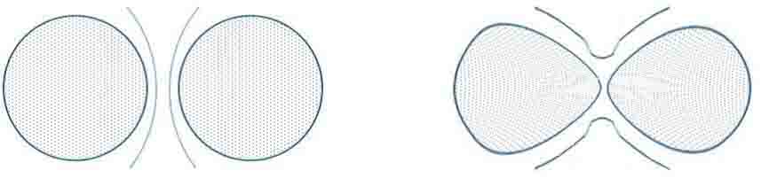
Figure 4: Interaction of two bubbles in pure liquid (interest to merging)

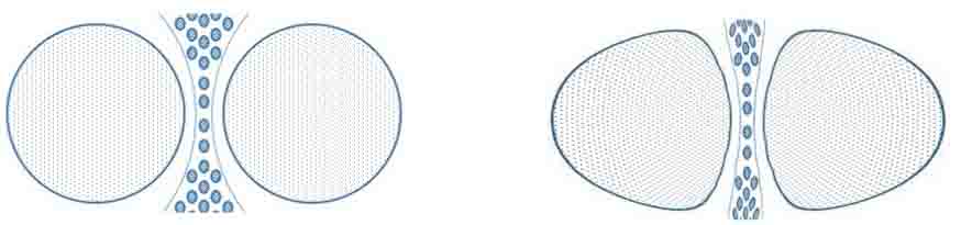
Figure 5: Interaction of two bubbles in melt liquid including solid particles (tolerate to merging)

To cover this phenomenon, some simple conditions are defined. First of all, it is assumed that each bubble interacts with liquid domain only, i.e. any numerical or logical conflicts between the bubbles are neglected. Secondly, each bubble possesses an interaction zone in the liquid phase as a result of its dynamic and velocity vectors. When these domains reach each other, the attracting force between the bubbles begins its performance. As mentioned earlier, a barrier of oxide-networks is formed between these domains that prevents bubbles’ coalescence. This effect could be modeled as an imaginary pressure in thin walls. By a simple condition the oxide-network effect can be simulated in the LBM code. This condition states in order to calculate corresponding Shan-Chen force at each lattice point when the interaction zones of bubbles collide, one would use the nearest bubble to that point and the effects of the rest of near bubbles are ignored, because their effect is practically neutralized by the oxide-network. This statement yields acceptable results in the final simulation. The modified Shan-Chen algorithm is represented in Fig. 6.

The computational procedure is conducted by two separate lattices, one for the melt and the other for the gas. This separation requires the utilization of the pseudopotential function, described in Eq. 30 and at the end of each time step, the lattices are coupled. Velocity and density at each lattice point is computed by Eq. 11.

Next step is the detection of the lattice points having the material between the melt and the gas (according to their velocity and density) and computing a new velocity for these points:

$$\textbf{u}_{total}=\frac{\textbf{u}_{melt}+\textbf{u}_{gas}}{\sum\rho}$$ (36)

Now the interaction potential could be calculated at each lattice point of the phases:

$$\xi=\rho c_{s}^{2}+\frac{G}{6}\psi^{2}$$ (37)

The final stage is to compute the velocities according to the calculated interaction potential and the external forces. But in the modified model, a correction is applied on the computed values. New lattices are created for each bubble, and contribution of each lattice (i.e. each bubble) to the velocity of the desired point in liquid lattice is computed:

$$\xi_{gas}=\left\{\begin{array}[]{l l}0&\qquad\sum_{k=1}^{n}|\xi_{k}|=0\\[7.22743pt] Max\left(\xi_{1},\cdots,\xi_{n}\right)&\qquad\frac{Max\left(|\xi_{1}|,\cdots,|\xi_{n}|\right)}{Max\left(\xi_{1},\cdots,\xi_{n}\right)}=1\\[7.22743pt] Min\left(\xi_{1},\cdots,\xi_{n}\right)&\qquad\frac{Max\left(|\xi_{1}|,\cdots,|\xi_{n}|\right)}{Max\left(\xi_{1},\cdots,\xi_{n}\right)}\neq 1\end{array}\right.$$ (38)

where $n$ is the number of bubbles in the domain. And the final velocities could be calculated:

$$\textbf{u}_{gas}=\textbf{u}_{total}+\tau_{gas}\left(F_{gas}-G\xi_{melt}\right)$$ (39)

$$\textbf{u}_{melt}=\textbf{u}_{total}+\tau_{melt}\left(F_{melt}-G\xi_{gas}\right)$$ (40)

Figure 6: Modified Shan-Chen Algorithm (Green: User Codes, Red: Open Source Codes)

When the interaction condition is applied to simulate the oxide network, the bubbles would never cross the oxide network barrier and no coalescence occurs in the main domain. To solve this problem, another condition should be defined. If this condition is defined based on experimental data, it would dictate if the distance between two bubbles reach a critical number, the oxide network wall condition would be removed, which leads the normal procedure of bubble dynamics to proceed. In mathematical and computational declarations, various variables could be processed in each time step in order to determine when to remove the wall condition. In this study, the pressure field and its second derivative in normal direction are the chosen criteria to develop a condition to model removal of thin film and bubble coalescence. This condition is removing the wall when the second derivative of pressure equals zero:

$$\eta_{m}=\left\{\begin{array}[]{l l}1&\quad\frac{d^{2}p}{dn^{2}}\neq 0\\[7.22743pt] 0&\quad\frac{d^{2}p}{dn^{2}}=0\end{array}\right.$$ (41)

By this removal of interaction condition, bubbles rapidly merge and their dynamic effect on liquid domain could be observed.

3 Experimental model

3.1 Foam formation dynamics

Metal foams consist of bubbles solidified just before the coalescence stage.

Bubble coalescence is an important step in foam formation process, in which the bubbles are merged by two different mechanisms. The first mechanism is the diffusion of gas from small bubbles to the bigger ones, known as Oswald Ripening, and is more understandable. The second mechanism is thin wall rupture. A thin film is formed between the bubbles while approaching each other. The characteristic of this thin film is the same as the continuous phase; for example, in aqueous solutions, the interaction of surfactants in bubble surface is the reason of the existence of this film [14].

The behavior of bubbles depends on the low-range and high-range forces which are the result of the type of surfactant, temperature and other components in the solution. In aqueous solutions, this mechanism depends primarily on the type of surfactant and it has little dependence on the characteristic of the phases. However, in some cases, such as air bubbles in oil, where the van-der Waals forces have low contribution in the interaction, the mechanism is different. In these solutions, the surfactants would be replaced by stabilizers. Presence of suspended impurity particles could result in a delay in coalescence stage [14].

Thin film rupture phenomena would be described in two different mechanisms. One of these mechanisms is the nucleation of a void and its growth due to surface tension forces. In this theory, in micro scale, a hole is formed randomly in the thin film. This formation consumes the energy $E_{r}$ ($2\pi\Gamma r-2\pi\gamma r^{2}$). If the size exceeds the critical radius $r^{*}$ ($\frac{\gamma}{2\Gamma}$), then stability is expected for the formed void, but in sizes less than the critical value, the void would be removed. Thus this mechanism requires activation energy $E_{a}=E(r^{*})$ to start, i.e. the nucleation of void is a thermal activated mechanism and would be described by Arrhenius equation [14].

The second mechanism, which is one of the considerations in present study, considers an instability similar to Spinodal decomposition. In this mechanism, if the thickness of the thin film falls below a critical value due to drainage, a perturbation will occur. Now the instability in the thin film is appeared as the wavelength of this vibration, exceeding the critical wavelength, which leads to the rupture of the film. This critical wavelength would be calculated as below:

$$\lambda_{c}=\sqrt{\frac{-2\pi^{2}\gamma}{d^{2}V/dh^{2}}}$$ (42)

where $\gamma$ is the surface energy and $V(h)$ the free energy of interface as a function of the thickness. If one considers the thin film as a cylinder with radius $R_{f}$ and thickness $h$ which is enclosed by two interface with surface tension $\gamma$, then the critical thickness of drainage would be:

$$h_{c}=0.22\sqrt[4]{\frac{AR_{f}^{2}}{f\gamma}}$$ (43)

As the thin film thickness reaches this value, the rupture will occur. The time taken from the instability to the rupture could be calculated too:

$$\tau=\frac{96\pi^{2}\gamma\eta h_{c}^{5}}{A^{2}}$$ (44)

If the limitation could be neglected, the thickening would continue up to the formation of a molecular wall. But in the presence of stabilizer particles, surfactants or oxide films, there would be a different situation. The described mechanism is more suitable for rapid growth, in which the system has no surfactant. Consequently, this mechanism is appropriate to be used in present investigation.

In metal melts, the oxide films and stabilizer particles are presented, which means it’s more probable for the second mechanism to occur. Thus one of the objectives of developed code is to model the instability in the thin wall formed between the bubbles.

3.2 Foam production

To study the structure of a porous metal foam, Formgrip method is chosen to produce aluminum metal foam. This method is a combination of powder metallurgy and melting method. At first, precursor of $A356$with $TiH_{2}$ is produced by melting. Then the precursor containing bubble nuclei is placed in a mold and is heated in furnace. Near the liquidus temperature, the precursor suddenly begins to blow. Bubble growing continues until they reach each other and before coarsening stage, the part is solidified. Then it is prepared for metallography images from cross-section of $A356$ foam after etching process. Finally, the experimental metallography images will be compared with bubbles images obtained from a simulation code that is developed in the present study. Also accuracy of the present code is evaluated as quantitative.

For producing the precursor, around 350g aluminum 356 alloy is melted in the furnace, around 1.5 %wt. blowing agent is mixed with aluminum powder with fraction of 0.5. For improving blowing agent wetting property in aluminum alloy melt and better uniform distribution, at 700 ${}^{\circ}C$ the blowing agent mixture is added to the melt. In the next step, the furnace temperature is set to 600 ${}^{\circ}C$. When the temperature reaches 620 ${}^{\circ}C$, the mixer rpm is set to 1500 and stirs for 1-2 min. In this step, more stirring causes more gas release. The resulting melt is rapidly casted into a metal mold.

The produced solid is called precursor. The precursor is cut for foaming process according to the mold size (a cylinder with a radius of 40mm and 80mm height). Then the mold and the precursor are heated in furnace to blow. In the present study, the effect of blowing temperature on the stability of foam for 675, 725 and 775 ${}^{\circ}C$ is investigated. For each temperature, 2-3 samples are produced to estimate the optimized foam processing time for producing foam with minimum density and stable cell structure. Schematic of foam producing steps is shown in Fig. 7.

Figure 7: Schematic of foam producing steps in formgrip method

3.3 Experimental test and validation

In order to determine the accuracy of the simulation results, simulated cellular structure of the present code have been compared with the experimental results. Thus, following the production of $A356$ foam, samples were sliced and mounted by black epoxy resin. For this purpose, the samples were washed with alcohol, then heated up by a dryer for better resin penetration in the foam cells, and are finally mounted. After curing, the samples’ surfaces are polished with 230 to 800 grit sandpapers. Samples’ surfaces need to be polished in order to give a clear picture of cellular structures. Images of samples cross sections are taken by SONY digital camera with 300dpi resolution.

4 Results

The coarsening of two in line bubbles shown in Fig. 8 without gravity have been simulated by two different methods. Fig. 9 shows the results of the interaction between two bubbles simulated by COMSOL commercial software using finite element method and level-set model. Results of LB method with OpenLB open source code is shown in Fig. 10. Multiphase model is Shan-Chen and lattice is D2Q9. Simulation conditions can be seen in Table.1.

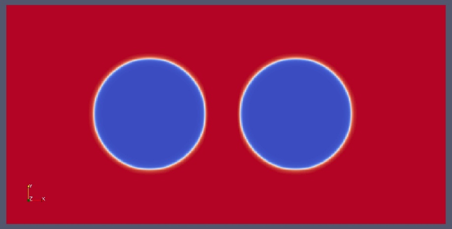
Figure 8: Initial state of the validation simulation, two gas bubble in aluminum melt

Table 1: Simulation condition for two in line bubbles

		COMSOL	OpenLB
Domain dimension (mm)		$20\times 30$	$20\times 30$
Fluid density ($\frac{g}{cm^{3}}$)		2.7	2.7
Gas density ($\frac{g}{cm^{3}}$)		0.089	0.089
Initial condition	Melt	$V=0\>mm/s$	$V=0\>mm/s$
		$P=1\>atm$	$P=1\>atm$
		$\mu=1.10\times 10^{-3}\>N.s/m^{2}$	$\mu=1.10\times 10^{-3}\>N.s/m^{2}$
	Bubble	$V=3\>mm/s$	$V=3\>mm/s$
		$P=1\>atm$	$P=1\>atm$
		$\mu=1.87\times 10^{-5}\>N.s/m^{2}$	$\mu=1.87\times 10^{-5}\>N.s/m^{2}$
Boundary condition		Slip	Mirror
Initial bubbles D (mm)		8	8
Final bubbles D (mm)		11.29	11.30

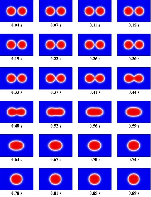
Figure 9: Simulation of two inline bubbles by finite element method and level set model in COMSOL package

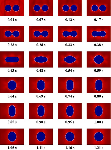
Figure 10: Simulation of two inline bubbles by LB method and Shan-Chen multiphase model in OpenLB open source code

In present study, modified Shan-Chen model in LB method is used to simulate the behavior of two in line bubbles in a foam like situation. Simulation conditions are listed in Table. 2 and results are shown in Fig. 11. In Fig. 12, the result of the pressure and velocity fields is demonstrated by the plot of the values across a vertical line, before and after the instability caused by the perturbation field of the interacting bubbles.

Table 2: Simulation condition for two inline bubbles by LB method and modified Shan-Chen model

		OpenLB
Domain dimension (mm)		$45\times 45$
Fluid density ($\frac{g}{cm^{3}}$)		2.7
Gas density ($\frac{g}{cm^{3}}$)		0.089
Initial condition	Melt	$V=0\>mm/s$
		$P=1\>atm$
		$\mu=1.10\times 10^{-3}\>N.s/m^{2}$
	Bubble	$V=3\>mm/s$
		$P=1\>atm$
		$\mu=1.87\times 10^{-5}\>N.s/m^{2}$
Boundary condition		Mirror
Initial bubbles D (mm)		8
Final bubbles D (mm)		11.30

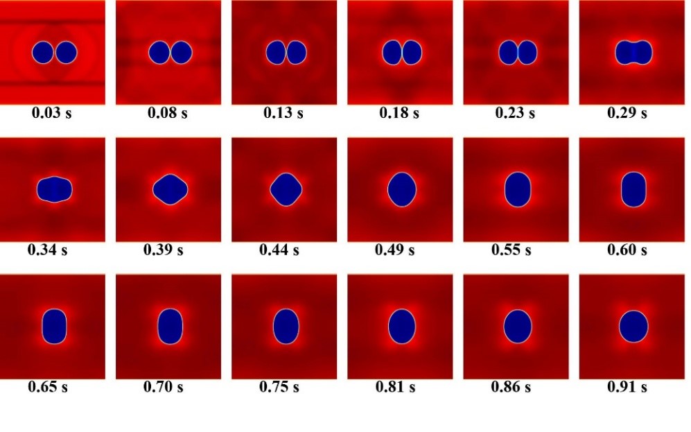
Figure 11: Coarsening simulation of two in line bubbles by LB method and modified Shan-Chen multiphase model in OpenLB

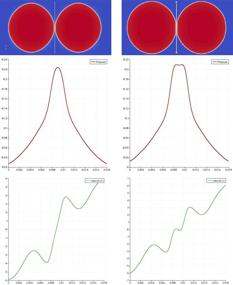
Figure 12: Plot of pressure and velocity across a vertical line in the middle of two bubbles. Left: before instability, Right: after instability. Red line indicates the pressure and green line is vertical velocity.

The Simulation results of bubble growth in a small domain of closed-cell aluminum foam structure with 6 primary bubbles in the mirror boundary conditions are shown in Fig. 13 and the simulation data are listed in Table. 3. In Fig. 14 magnified picture of aluminum foam cellular structure is shown to evaluate the accuracy of this study’s code in regards to the detection of cell wall thinning stage in bubble coarsening (see top right of Fig. 14). Small domain of Fig. 14, as mentioned before is simulated by mirror boundary condition which dictates that if any melt comes out of a wall it has to come from an opposite one. Thus, by repeating the simulated mirror domain, domain of a few millimeters can be transformed, by a good approximation, to a several centimeters domain. The result of such repetitions is shown in Fig. 15. Blue and red color of phase contours have been changed to gray scale to resemble the color of aluminum foam cross sections. In this case, it could be assumed that the speed of solidification is fast enough to freeze the molten aluminum foam into solid state as the cell structure maintains its molten state. Thus Fig. 15 can be a part of a solid aluminum foam structure. In other words, Fig. 15 can be considered as a simulation metallography picture of porous aluminum foam structure. Fig. 16 shoes the experimental metallography pictures of aluminum $A356$ foam that produced by Formgrip method in 675, 725 and 775 ${}^{\circ}C$, for comparison with the simulated metallographic pictures. The results of this comparison are shown in Fig. 17 and 18.

Table 3: Simulation conditions of small domain of metal foam by LB method and modified Shan-Chen model

		OpenLB
Domain dimension (lattice parameter)		$750\times 500$
Fluid density ($\frac{g}{cm^{3}}$)		2.7
Gas density ($\frac{g}{cm^{3}}$)		0.089
Initial condition	Melt	$\mu_{675}=1.20\times 10^{-3}\>N.s/m^{2}$
		$\mu_{725}=1.10\times 10^{-3}\>N.s/m^{2}$
		$\mu_{775}=1.02\times 10^{-3}\>N.s/m^{2}$
	Bubble	$\mu_{675}=1.82\times 10^{-5}\>N.s/m^{2}$
		$\mu_{725}=1.87\times 10^{-5}\>N.s/m^{2}$
		$\mu_{775}=1.93\times 10^{-5}\>N.s/m^{2}$
Boundary condition		Mirror

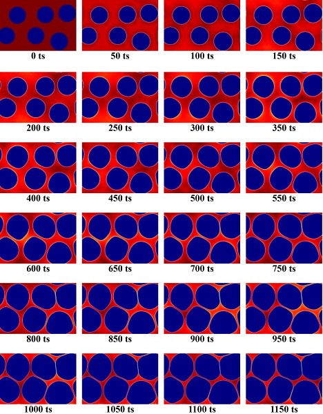
Figure 13: Simulation results of foaming stage for small domain of metal foam by LB method and modified Shan-Chen model with mirror boundary condition in OpenLB

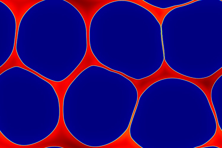
Figure 14: Bubble cell walls thinning simulation during growth step of a small foam domain (top left bubbles)

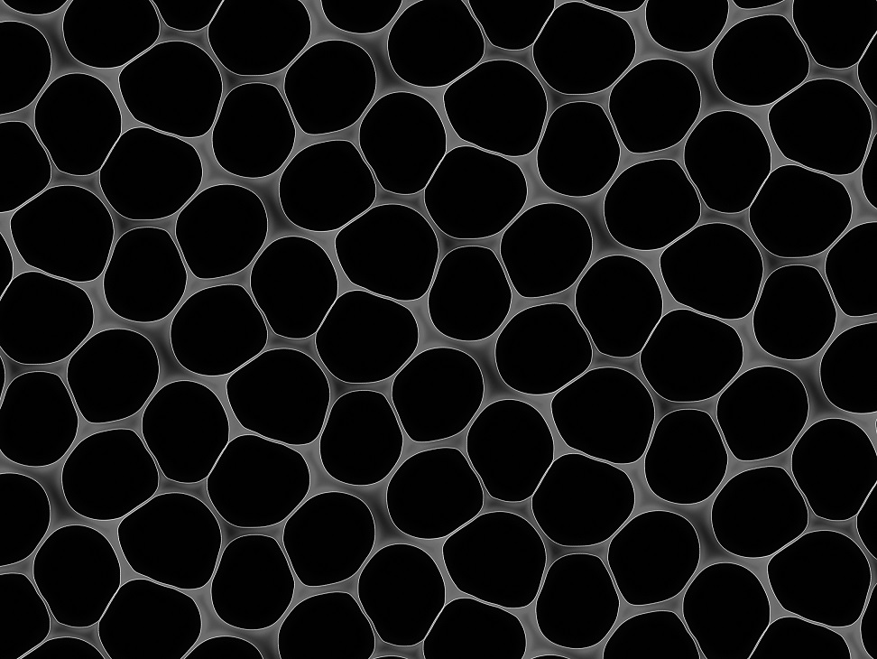
Figure 15: Imaginary metallographic structure of porous aluminum metal foam that created from mirror repeating of Fig. 14

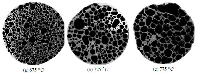
Figure 16: Metallographic image of aluminum A356 metal foam

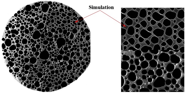
Figure 17: Experimental and simulation metallographic structure of aluminum metal foam produced by formgrip in 675 ${}^{\circ}C$

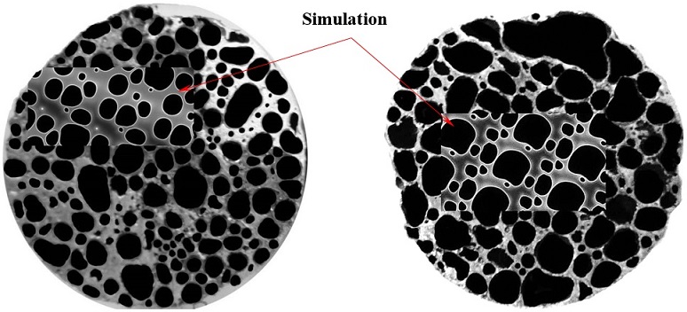
Figure 18: Experimental and simulation metallographic structure of aluminum A356 foam (left: 725 ${}^{\circ}C$ and right: 775 ${}^{\circ}C$)

5 Discussion

In Lattice Boltzmann method, the macroscopic properties of the domain of interest could be predicted by solving the LB equations at mesoscopic scale. In this investigation, this numerical method is used and the Shan-Chen scheme for multiphase modeling is modified to present a code to predict the behavior of metal foams. In available commercial CFD codes, the modeled behavior of bubbles is not similar to the dynamics seen in experimental observation. By modifying the Shan-Chen model (which is one the most accurate models in multiphase LB simulations), improved results in field of bubble dynamics would be achieved.

In order to validate and compare the developed code, two bubbles at growth stage in a container are considered and the dynamics of interaction is determined by using a conventional CFD code, unmodified LB code and present code. The boundaries of the domain are assumed to be closed for the gas phase and opened for the liquid phase, which causes the extra liquid exit the domain as the gas bubbles grow. The interaction begins as the volume of the bubbles increases. The initial state of this model is represented in Fig. 8.

According to Fig. 9 and Fig. 10, obtained simulation results from the LBM method with unmodified Shan-Chen model by OpenLB code, and the FEM with level set model by COMSOL software have a same behavior during interaction of two bubbles. In both methods, as the bubbles collide, a tip is formed on bubbles boundary at the interface zone between two bubbles. This shows the absorption force of bubbles that moves bubbles toward each other for merging and decreasing surface energy. Obtained quantitative results from both simulations listed in Table. 4.

Table 4: Simulation result comparison for two in line bubbles

	COMSOL	OpenLB	Modified code
Boundary condition	Slip	Mirror	Mirror
Initial bubbles D (mm)	8	8	8
Final bubbles D (mm)	11.29	11.30	11.30
Merging time (s)	0.26	0.25	0.31

These results are factual for every liquid without any solid impurity. But as mentioned before this behavior is not acceptable for metals melt, especially in aluminum and aluminum alloys foaming process. In metals there is no tip at the intersection of two bubbles. Therefore, for bubbles growth in metal melt, a new model should be developed. In this study, this objective is accomplished by using a modified version of the Shan-Chen model in LBM simulation of metal foaming process. The result of the simulation performed using this new code for aluminum melt compared with COMSOL and OpenLB software is shown in Table. 4. The result shown in Fig. 10 means that the bubble dynamics equations are well satisfied and the result domain shows behavior based on these equations. But the behavior of bubbles in the interaction is not the one expected from metal melts due to the presence of impurities and the particles-network as discussed before. In Fig. 11, simulation results illustrated based on the modified Shan-Chen model. As shown, in this figure, at interface of the bubble interaction, a thin film is formed and the merging phenomenon does not occur until a specific criterion is met.

Furthermore, to complete the validation results of the developed code, the pressure and velocity values across a vertical line is shown in Fig. 12. It is observed that for a specific thickness an instability will occur, which is dependent on the size of the bubbles. This instability could be seen in the pressure profile (right image of Fig. 12). Thus, in the beginning of the instability, the second derivative of pressure ($\nabla^{2}P$) profile in the lattice point would be zero, which indicates the initialization of bubbles wall rupture. Then it is possible and more comfortable to determine the wall rupture by using the pressure profile and pressure second derivative instead of detecting the critical thickness. By applying this criterion to the domain of foam formation, the merge condition of the gas bubbles would be detected based on the second derivative of pressure field at each lattice points, which leads to an improved modeling of metal foam formation process.

Designing an experiment that could show the dynamics of two moving bubbles in aluminum melt to validate present simulation is very expensive and requires very especial equipment for casting and would be impossible due to non-transparent molten metals. In Fig. 15 shows simulation results of a cross-section of A356 foam based on the modified Shan-Chen method at present code. In this image, a small portion of the domain has been repeated by using periodic boundary condition.

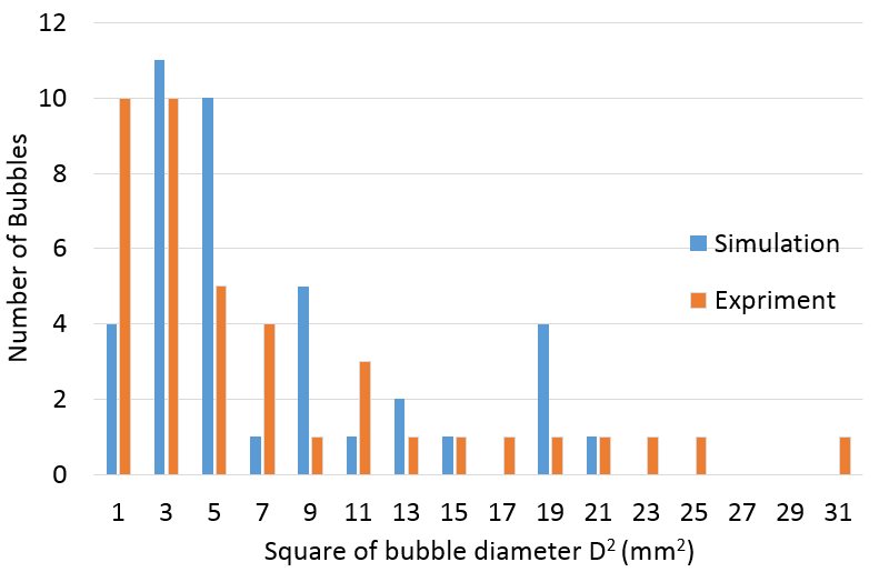
Figure 19: Bubble size distribution of simulation and experimental samples of Fig. 17

Table 5: Comparison of extracted data from simulation and experimental metallographic cellular structures of Fig. 17

	simulation	experimental	Error
Bubble percentage	44.3%	45.5%	2.64%
Foam Density ($\frac{g}{cm^{3}}$)	1.50	1.47	2.04%
Mean bubble size (mm)	3.03	3.05	0.66%

Fig. 13 shows foaming stage for small domain of metal foam by time. Bubbles with random distribution began to grow after nucleation. Bigger bubbles have a higher growth rate than the others. Each bubble has an affected zone, and when these zones reach each other, bubbles interaction will begin. Simulation of bubbles’ growth will continue until first cell reaches the wall rupture criterion as like Fig. 14. After this time (best foaming time), foaming simulation process would suddenly enter the aging step and bubbles coalescence, which leads to a sever drainage in metal foam structure. These simulation metallography images could be used for predicting of experimental metallography images (as like Fig. 16) and optimum foaming time. These comparisons are represented in Fig. 17 for 675 ${}^{\circ}C$ and Fig. 18 for 725 and 775 ${}^{\circ}C$, respectively. In addition to visual results, quantitative results are extracted from Fig. 17 simulation data in order to validate. These extracted results are processed by using MATLAB image processor and are illustrated in Fig. 19 and Table. 5. These data show a minor error between the simulation and the experiment results. Therefore, present code based on modified Shan-Chen model and LB method could simulate and predict foamy structures for aluminum $A356$ foams during isothermal foaming process.

6 Conclusions

In this investigation, the Lattice Boltzmann Method (LBM) was utilized for understanding of foaming process by simulation of different stages of the Aluminum A356 foam production process at micro and meso scales. Therefore, to predict the structure of metal foam during foaming process, a model is established to simulate the dynamics of bubbles interaction based on development of Shan-Chen model. The presented model can consider the effect of the attraction-repulsion barriers among bubbles into the A356 aluminum foam liquid due to the solid particles network. In order to validate the presented model, results were compared by both some other reference codes and experimental data. Comparison of cellular structure obtained from the experimental route (experimental metallography) and the numerical code (simulation metallography) shows a good consistency. The presented code is also capable of simulating and presenting virtual metallography images for all aluminum alloys foams. Therefore, this software can be used for controlling and predicting density of foams combined with uniform distribution of bubbles at the metal foams.

References

- Banhart [2000] Banhart J. Manufacturing routes for metallic foams. Journal of The Minerals, Metals & Materials Society 2000;52(12):22–7.
- Banhart [2001] Banhart J. Manufacture, characterization and application of cellular metals and metal foams. Progress in Materials Science 2001;46:559–632.
- Banhart et al. [1995] Banhart J, j. Baumeister , Weber M. Powder metallurgical technology for the production of metallic foams. In: European Conference on Advanced PM Materilas. Brimimgham; 1995:201–8.
- Körner [2008a] Körner C. Integral Foam Molding of Light Metals. Springer; 2008a.
- Körner [2008b] Körner C. Foam formation mechanisms in particle suspensions applied to metal foams. Materials Science and Engineering A 2008b;495:227–35.
- Stanzick et al. [2002] Stanzick H, Wichmann M, Weise J, Helfen L, Baumbach T, Banhart J. Process control in aluminum foam production using real-time x-ray radioscopy. Advanced Engineering Materials 2002;4(10):814–23.
- Körner et al. [2005] Körner C, Arnold M, Singer RF. Metal foam stabilization by oxide network particles. Materials Science and Engineering A 2005;396:28–40.
- Brennen [1995] Brennen CE. Cavitation and bubble dynamics. Oxford University Press; 1995.
- Chine and Monno [2011] Chine B, Monno M. Multiphysics modeling of a gas bubble expansion. In: Proceedings of 2011 European COMSOL Conference. 2011:.
- Chahine and Duraiswami [1992] Chahine GL, Duraiswami R. Dynamical interactions in a multi-bubble cloud. Fluids Eng 1992;114(4):680–6.
- Chahine [1994] Chahine GL. Strong interactions bubble/bubble and bubble/flow. In: Bubble Dynamics and Interface Phenomena; vol. 23 of Fluid Mechanics and Its Applications. Springer Netherlands; 1994:195–206.
- Ida [2009] Ida M. Bubble-bubble interaction: A potential source of cavitation noise. Phys Rev E 2009;79:016307.
- Bremond et al. [2006] Bremond N, Arora M, Dammer SM, Lohse D. Interaction of cavitation bubbles on a wall. Physics of Fluids 2006;18(12).
- Bibette et al. [1999] Bibette J, Calderon FL, Poulin P. Emulsions: basic principles. Rep Prog Phys 1999;62:969–1033.
- Ghosh et al. [2012] Ghosh S, Das AK, Vaidya AA, Mishra SC, Das PK. Numerical study of dynamics of bubbles using lattice Boltzmann method. Industrial & Engineering Chemistry Research 2012;51(18):6364–76.
- Kim et al. [2010] Kim Y, Lai MC, Peskin CS. Numerical simulations of two-dimensional foam by the immersed boundary method. Journal of Computational Physics 2010;229(13):5194 –207.
- Gupta and Kumar [2008] Gupta A, Kumar R. Lattice Boltzmann simulation to study multiple bubble dynamics. International Journal of Heat and Mass Transfer 2008;51(21-22):5192 –203.
- Anderl et al. [2014] Anderl D, Bauer M, Rauh C, Rüde U, Delgado A. Numerical simulation of adsorption and bubble interaction in protein foams using a lattice Boltzmann method. Food Funct 2014;5:755–63.
- Leung et al. [2006] Leung SN, Park CB, Xu D, Li H, Fenton RG. Computer simulation of bubble-growth phenomena in foaming. Industrial & Engineering Chemistry Research 2006;45(23):7823–31.
- Beugre et al. [2010] Beugre D, Calvo S, Dethier G, Crine M, Toye D, Marchot P. Lattice boltzmann 3d flow simulations on a metallic foam. Journal of Computational and Applied Mathematics 2010;234(7):2128 –34.
- Diop et al. [2011] Diop M, Hao H, Dong HW, Zhang XG, Yao S, Jin JZ. Modelling of solidification process of aluminum foams using lattice Boltzmann method. International Journal of Cast Metals Research 2011;24:158–62.
- John and Anderson [1995] John D, Anderson J. Computational Fluid Dynamics: The Basics with Application. McGraw Hill; 1995.
- Succi [2001] Succi S. The Lattice Boltzmann Equation f or Fluid Dynamics and Beyond. Oxford University Press; 2001.
- Grunau et al. [1993] Grunau D, Chen S, Egger K. A lattice boltzmann model for multiphase fluid flows. Physics of Fluids A 1993;5(10):2557–62.
- Shan and Chen [1993] Shan X, Chen H. Lattice Boltzmann model for simulating flows with multiple phases and components. Physical Review E 1993;47(3):1815–9.
- Shan and Chen [1994] Shan X, Chen H. Simulation of nonideal gases and liquid-gas phase transitions by the lattice Boltzmann equation. Physical Review E 1994;49(4):2941–8.
- Swift et al. [1995] Swift MR, Orlandini E, Osborn WR, Yeomans JM. Lattice Boltzmann simulation of nonideal fluids. Physical Review E 1995;75(5):830–3.
- Swift et al. [1996] Swift MR, Orlandini E, Osborn WR, Yeomans JM. Lattice boltzmann simulations of liquid-gas and binary fluid systems. Physical Review E 1996;54(5):5041–52.
- Gunstensen et al. [1991] Gunstensen AK, Rothman DH, Zaleski S, Zanetti G. Lattice Boltzmann model for immiscible fluids. Physical Review A 1991;43(8):4320–7.
- He et al. [1998] He X, Shan X, Doolen GD. Discrete Boltzmann equation model for nonideal gases. Physical Review E 1998;57(1):R13–6.
- Chen et al. [1996] Chen S, Martinez D, Mei R. On boundary conditions in lattice boltzmann methods. Physics of Fluids 1996;8(9):2527–36.
- He and Lou [1997] He X, Lou S. Theory of the lattice botlzmann method: From the boltzmann equation to the lattice boltzmann equation. Physical Review E 1997;56(6):6811–7.
- Yuan and Schaefer [2006] Yuan P, Schaefer L. Equations of state in a lattice Boltzmann model. Physics of Fluids 2006;18:42101–11.
- Sbragaglia et al. [2007] Sbragaglia M, Benzi R, Biferali L, Succi S, Sugiyama K, Toschi F. Generalized lattice Boltzmann method with multirange potential. Physical Review E 2007;75:1–13.
- Inamuro et al. [1997] Inamuro T, Yoshino M, Ogino F. Accuracy of the lattice boltzmann method for small knudsen number with finite reynolds number. Physics of Fluids 1997;9(11):3535–42.
- He and Doolen [2002] He X, Doolen GD. Thermodynamic foundations of kinetic theory and lattice boltzmann models for multiphase flows. Journal of Statistical Physics 2002;117(112):309–28.
- Krause [2013] Krause MJ. OpenLB. open source code; 2013. Karlsruhe Institute of Technology.