High-fidelity state transfer through long-range correlated disordered quantum channels

Abstract

We study quantum-state transfer in $XX$ spin-$1/2$ chains where both communicating spins are weakly coupled to a channel featuring disordered on-site magnetic fields. Fluctuations are modelled by long-range correlated sequences with self-similar profile obeying a power-law spectrum. We show that the channel is able to perform an almost perfect quantum-state transfer in most of the samples even in the presence of significant amounts of disorder provided the degree of those correlations is strong enough. In that case, we also show that the lack of mirror symmetry does not affect much the likelihood of having high-quality outcomes. Our results advance a further step in designing robust devices for quantum communication protocols.

I Introduction

Transmitting quantum states and establishing entanglement between distant parties (say Alice and Bob) are crucial tasks in quantum information processing protocols Cirac et al. (1997); Kimble (2008). In this direction, spin chains have been widely addressed as quantum channels for (especially short-distance) communication protocols since proposed in Ref. Bose (2003) that spin chains can be used for carrying out transfer of quantum information with minimal control, i.e., no manipulation is required during the transmission. Basically, Alice prepares and sends out an arbitrary qubit state through the channel and Bob only needs to make a measurement at some prescribed time. The evolution itself is given by the natural dynamics of the system.

Since then, several schemes for high-fidelity quantum-state transfer (QST) Bose (2003); Christandl et al. (2004); Plenio et al. (2004); Osborne and Linden (2004); Wójcik et al. (2005); *wojcik07; Li et al. (2005); Huo et al. (2008); Gualdi et al. (2008); Banchi et al. (2010); *banchi11; *apollaro12; Lorenzo et al. (2013, 2015); Almeida et al. (2016) and entanglement creation and distribution Amico et al. (2004); Plenio and Semião (2005); Apollaro and Plastina (2006); *plastina07; *apollaro08; Campos Venuti et al. (2007); Cubitt and Cirac (2008); Giampaolo and Illuminati (2009); *giampaolo10; Gualdi et al. (2011); Estarellas et al. (2017a); *estarellas17scirep; Almeida et al. (2017) in spin chains have been put forward. For instance, it was discovered that perfect QST can be achieved in mirror-symmetric chains by a judicious tuning of the spin-exchange couplings over the entire chain Christandl et al. (2004); Plenio et al. (2004) (see Feder (2006) for a generalization). While this scheme allows one to perform QST with unit fidelity for arbitrarily-large distances, it is not an easy task, on the practical side, to engineer the whole chain with the desired precision, what makes this configuration very sensitive to perturbations De Chiara et al. (2005); Zwick et al. (2011); *zwick12. An alternative less-demanding approach is based on optimizing the outermost couplings of a uniform channel so that the linear part of the spectrum dominates the dynamics (Banchi et al., 2010). One can also encode the information using multiple spins to send dispersion-free Gaussian wave-packets through the channel Osborne and Linden (2004). Another class of protocols relies on setting very weak couplings between the end spins (those being the sender and receiver sites) and the bulk of the chain Wójcik et al. (2005); Li et al. (2005); Campos Venuti et al. (2007); Huo et al. (2008); Gualdi et al. (2008); Giampaolo and Illuminati (2009, 2010); Almeida et al. (2016) in order to effectively reduce the operating Hilbert space to that of a two- or three-site chain, depending on the resonance conditions. That way, it is possible to carry out QST with close-to-unit fidelity. A similar strategy is to apply strong magnetic fields at the sender and receiver spins (or on their nearest neighbors) Plastina and Apollaro (2007); Lorenzo et al. (2013); Paganelli et al. (2013).

Each of the aforementioned schemes has its own peculiarities but there is one detail that can seriously compromise the protocol regardless of the engineering scheme being used, that is disorder. Fluctuations either in the local magnetic fields or in the coupling strengths are inevitably present either due to manufacturing errors or dynamical spurious factors hence leaving us far from the desired output. Needless to say, finding out ways to overcome such difficulties and and testing the robustness of various schemes against such experimental imperfections are of great importance and have been done extensively De Chiara et al. (2005); Fitzsimons and Twamley (2005); Burgarth and Bose (2005); Tsomokos et al. (2007); Giampaolo and Illuminati (2010); Petrosyan et al. (2010); Yao et al. (2011); Zwick et al. (2011); Bruderer et al. (2012); Kay (2016). Among many possible configurations to realize high-quality QST, in the presence of disorder it should be much more preferable to choose a channel in which the sender and receiver spins do not heavily depend upon. Having that in mind, those setups featuring communicating parties weakly coupled to the channel Wójcik et al. (2005) seem to be a promising choice Yao et al. (2011). A combined approach involving modulated couplings with weakly coupled spins has been also put forward in Bruderer et al. (2012). Still, the slightest amount of disorder is already capable of promoting Anderson localization effects Anderson (1958); *abrahams79 or, even worse, destroying the symmetry of the channel Albanese et al. (2004). That is not necessarily true, however, in the case of correlated disorder. The breakdown of Anderson localization has been reported when short- Flores (1989); *dunlap90; *phillips91 or long-range correlations de Moura and Lyra (1998); Izrailev and Krokhin (1999); Kuhl et al. (2000); Lima et al. (2002); *demoura02; *nunes16; de Moura et al. (2003); Domínguez-Adame et al. (2003); Herrera-González et al. (2014); Almeida et al. (2017) are present in disordered 1D models. In particular, the latter case finds a set of extended states in the middle of the band with well detached mobility edges thereby signalling an Anderson-type metal-insulator transition de Moura and Lyra (1998); Izrailev and Krokhin (1999). This is also manifested in low-dimensional spin chains Lima et al. (2002); Almeida et al. (2017).

Correlated fluctuations takes place in many stochastic processes in nature (see, e.g., Refs. Lam and Sander (1992); Peng et al. (1992); Carreras et al. (1998); Carpena et al. (2002)) and therefore shall not be ruled out when designing protocols for quantum information processing in solid-state devices De Chiara et al. (2005); Burgarth and Bose (2005). Here, we will see that it indeed makes a dramatic difference in the performance of QST protocols based on weakly-coupled end spins. Specifically, we consider an one-dimensional $XX$ spin chain in which the local magnetic fields (on-site potentials) of the channel follow a long-range correlated disordered distribution with power-law spectrum $S(k)\propto 1/k^{\alpha}$, with $k$ being the corresponding wave number and $\alpha$ being a characteristic exponent governing the degree of such correlations. We show that when perturbatively attaching two communicating (end) spins to the channel and setting their frequency to lie in the middle of the band, we are still able to perform nearly perfect QST rounds in the presence of correlated disorder. Surprisingly, it happens even in the presence of considerable amounts of asymmetries in the channel. The reason for that is the appearance of extended states in the middle of the band which offers the necessary end-to-end effective symmetry thereby supporting the occurrence of Rabi-like oscillations between the sender and receiver spins. We show that perfect mirror symmetry, despite being very convenient for QST protocols, is not a crucial factor as long as there exists a proper set of delocalized eigenstates in the channel.

In the following, Sec. II, we introduce the $XX$ spin Hamiltonian with on-site long-range correlated disorder. In Sec. III we derive an effective two-site Hamiltonian that accounts for the way both communicating parties are coupled to the channel. In Sec. IV we investigate how the channel responds to disorder by looking at the resulting effect on the localization and symmetry properties. In Sec. V we display the results for the QST fidelity and our final remarks are addressed in Sec. VI.

II Spin-chain Hamiltonian

We consider a pair of spins (communicating parties) coupled to a one-dimensional quantum channel consisting altogether of an open spin-$1/2$ chain featuring $XX$-type exchange interactions described by Hamiltonian $\hat{H}=\hat{H}_{\mathrm{ch}}+\hat{H}_{\mathrm{int}}$ with ($\hbar=1$)

$$\hat{H}_{\mathrm{ch}}=\sum_{i=1}^{N}\dfrac{\omega_{i}}{2}(\hat{1}-\hat{\sigma}_{i}^{z})-\sum_{\langle i,j\rangle}\dfrac{J_{i,j}}{2}(\hat{\sigma}_{i}^{x}\hat{\sigma}_{j}^{x}+\hat{\sigma}_{i}^{y}\hat{\sigma}_{j}^{y}),$$ (1)

where $\hat{\sigma}_{i}^{x,y,z}$ are the Pauli operators for the $i$-th spin, $\omega_{i}$ is the local (on-site) magnetic field, and $J_{i,j}$ is the exchange coupling strength between between nearest-neighbor nodes. Supposing the sender ($s$) and receiver ($r$) spins are connected to nodes $1$ and $N$ from the channel at rates $g_{s}$ and $g_{r}$, respectively, the interaction part reads

$$\hat{H}_{\mathrm{int}} =\dfrac{\omega_{s}}{2}(\hat{1}-\hat{\sigma}_{s}^{z})+\dfrac{\omega_{r}}{2}(\hat{1}-\hat{\sigma}_{r}^{z})$$ (2)

$$\quad-\dfrac{g_{s}}{2}(\hat{\sigma}_{s}^{x}\hat{\sigma}_{1}^{x}+\hat{\sigma}_{s}^{y}\hat{\sigma}_{1}^{y})+\dfrac{g_{r}}{2}(\hat{\sigma}_{r}^{x}\hat{\sigma}_{N}^{x}+\hat{\sigma}_{r}^{y}\hat{\sigma}_{N}^{y}).$$

Note that since $\hat{H}$ conserves the total magnetization of the system, i.e., $\left[\hat{H},\sum_{i}\hat{\sigma}_{i}^{z}\right]=0$, the Hamiltonian can be split into independent subspaces with fixed number of excitations. Here we focus on the single-excitation Hilbert space spanned by states of the form $|i\rangle=\hat{\sigma}_{i}^{+}|\downarrow\downarrow\ldots\downarrow\rangle$ with $i=r,s,1,\ldots,N$, that means every spin pointing down but the one located at the $i$-th position. In this case, we end up with a hopping-like matrix with $N+2$ dimensions. Indeed $\hat{H}$ can be mapped onto a system describing non-interacting spinless fermions through the Jordan-Wigner transformation.

Let us now make a few assumptions in regard to the channel described by Hamiltonian (1). Here we consider the spin-exchange coupling strengths to be uniform $J_{i,j}\rightarrow J$ and, in order to study the robustness of the channel against disorder we introduce correlated static fluctuations on the on-site magnetic field $\omega_{n}$, $n=1,\ldots,N$. A straighforward way to generate random sequences featuring internal long-range correlations is through the trace of the fractional Brownian motion with power-law spectrum $S(k)\propto 1/k^{\alpha}$ de Moura and Lyra (1998); Domínguez-Adame et al. (2003)

$$\omega_{n}=\sum_{k=1}^{N/2}k^{-\alpha/2}\mathrm{cos}\left(\dfrac{2\pi nk}{N}+\phi_{k}\right),$$ (3)

where $k=1/\lambda$, is the inverse modulation wavelength, $\{\phi_{k}\}$ are random phases distributed uniformly within $\left[0,2\pi\right]$, and $\alpha$ controls the degree of correlations. This parameter is related to the so-called Hurst exponent Feder (1988), $H=(\alpha-1)/2$, which characterizes the self-similar character of a given sequence. When $\alpha=0$, we recover the case of uncorrelated disorder (white noise) and for $\alpha>0$ underlying long-range correlations take place. The resulting long-range correlated sequence becomes nonstationary for $\alpha>1$. Furthermore, according to the usual terminology, when $\alpha>2$ ($\alpha<2$) the series increments become persistent (anti-persistent). Interestingly, this brings about serious consequences on the spectrum profile of the system. As shown in de Moura and Lyra (1998); Domínguez-Adame et al. (2003), when $\alpha>2$ there occurs the appearance of delocalized states in the middle of the one-particle spectrum band. In the QST scenario with weakly-coupled spins $r$ and $s$, i.e. $g_{s},g_{r}\ll J$, that promotes a strong enhancement in the likelihood of disorder realizations with very-high fidelities $F$, most of them yielding $F\approx 1$. This will be elucidated along the paper.

Hereafter we set the sequence generated by Eq. (3) to follow a normalized distribution, that is $\omega_{n}\rightarrow\left(\omega_{n}-\langle\omega_{n}\rangle\right)/\sqrt{\langle\omega_{n}^{2}\rangle-\langle\omega_{n}\rangle^{2}}$. We also stress that such a disordered distribution has no typical length scale which is a property of many natural stochastic series Paczuski et al. (1996).

III Effective two-site description

We now work out a perturbative approach to write down a proper representation of an effective Hamiltonian involving only the sender and receiver spins provided they are very weakly coupled to the channel. Intuitively, we expect they span their own subspace with renormalized parameters and thus QST takes place via effective Rabi oscillations between them Wójcik et al. (2005); Gualdi et al. (2008); Lorenzo et al. (2013); Almeida et al. (2016). Our goal here is to investigate the influence of disorder in such subspaces and see about how much asymmetry they are able to tolerate.

Here, we follow the procedure adopted in Refs. Wójcik et al. (2007); Li et al. (2005). To begin with, let us express the channel Hamiltonian, Eq. (1), in terms of its eigenstates $\{|E_{k}\rangle\}$ with corresponding (nondegenerate) frequencies $\{E_{k}\}$ and recast $\hat{H}=\hat{H}_{0}+\hat{V}$, such that

$$\hat{H}_{0}=\omega_{s}|s\rangle\langle s|+\omega_{r}|r\rangle\langle r|+\sum_{k}E_{k}|E_{k}\rangle\langle E_{k}|,$$ (4)

$$\hat{V}=\epsilon\sum_{k}\left(g_{s}a_{sk}|s\rangle\langle E_{k}|+g_{r}a_{rk}|r\rangle\langle E_{k}|+\mathrm{H.c.}\right)$$ (5)

are now the free and perturbation Hamiltonians, respectively, with $\epsilon$ being a perturbation parameter, $a_{sk}\equiv\langle 1|E_{k}\rangle$, and $a_{rk}\equiv\langle N|E_{k}\rangle$. Herein we set units such that $J=1$ for convenience.

If we consider that both $\omega_{s}$ and $\omega_{r}$ do not match any of the normal frequencies $E_{k}$ of the channel and set $\epsilon g_{s}$ and $\epsilon g_{r}$ to be very weak so as to not disturb the nearby modes, we expect reaching an effective Hamiltonian of the form $\hat{H}_{\mathrm{eff}}=\hat{H}_{\mathrm{ch}}\oplus\hat{H}_{sr}$ up to some leading order in $\epsilon$, where $\hat{H}_{sr}$ is the decoupled two-spin Hamiltonian which contains all the valuable information on the way the sender and receiver spins “feel” the spectrum of the channel. The trick to find $\hat{H}_{\mathrm{eff}}$ is quite straightforward Wójcik et al. (2007). Suppose there is a transformation $\hat{H}_{\mathrm{eff}}=e^{i\hat{S}}\hat{H}e^{-i\hat{S}}$, with $\hat{S}$ being a Hermitian operator which we properly choose to be of the form

$$\hat{S}=i\epsilon\sum_{k}\left(\dfrac{g_{s}a_{sk}}{E_{k}-\omega_{s}}|s\rangle\langle E_{k}|+\dfrac{g_{r}a_{rk}}{E_{k}-\omega_{r}}|r\rangle\langle E_{k}|+\mathrm{H.c.}\right).$$ (6)

This choice is very convenient because it rules out the first order terms $\hat{V}+i[\hat{S},\hat{H}_{0}]=0$ and, up to second-order perturbation theory, we are then left with

$$\hat{H}_{\mathrm{eff}}=\hat{H}_{0}+i[\hat{S},\hat{V}]+\dfrac{i^{2}}{2!}[\hat{S},[\hat{S},\hat{H_{0}}]]+O(\epsilon^{3}).$$ (7)

By inspecting the above equation, we see that spins $r$ and $s$ are now decoupled from the rest of the chain, as we intended to. The corresponding Hamiltonian projected onto $\{|s\rangle,|r\rangle\}$ then reads

$$\hat{H}_{sr}=\begin{pmatrix}h_{s}&-J^{\prime}\\ -J^{\prime}&h_{r}\end{pmatrix},$$ (8)

with

$$h_{\nu}=\omega_{\nu}-\epsilon^{2}g_{\nu}^{2}\sum_{k}\dfrac{|a_{\nu k}|^{2}}{E_{k}-\omega_{\nu}},$$ (9)

$\nu\in\{s,r\}$, and

$$J^{\prime}=\dfrac{\epsilon^{2}g_{s}g_{r}}{2}\sum_{k}\left(\dfrac{a_{sk}a_{rk}}{E_{k}-\omega_{s}}+\dfrac{a_{sk}a_{rk}}{E_{k}-\omega_{r}}\right).$$ (10)

Note that we are assuming all parameters to be real. Hamiltonian (8) describes a two-level system which performs Rabi-like oscillations in a time scale set by the inverse of the gap between its normal frequencies. In order to have as perfect as possible QST one should guarantee that $h_{s}=h_{r}$. This is automatically fulfilled, given $\omega_{s}=\omega_{r}$ and $g_{s}=g_{r}=g$, for mirror-symmetric chains since $|a_{sk}|=|a_{rk}|$ for every $k$. In that case, for a noiseless uniform channel and in the limit of very weak outer couplings, which implies in the validity of Hamiltonian (8), an initial state prepared in $|s\rangle$ will evolve in time to $|r\rangle$ with nearly unit amplitude at times $\tau J=n\pi/(2J^{\prime})=n\pi/(2\epsilon^{2}g^{2})$, with $n$ being an odd integer Wójcik et al. (2005, 2007). Note that as $N$ increases more eigenstates get in the middle of the spectrum and thus $\epsilon g_{\nu}$ must be adjusted accordingly (we shall drop out the perturbation parameter $\epsilon$ hereafter).

In summary, in Rabi-type QST protocols Wójcik et al. (2005); Gualdi et al. (2008); Lorenzo et al. (2013); Almeida et al. (2016), a pair of eigenstates of the form $|\psi^{\pm}\rangle\approx(|s\rangle\pm|r\rangle)/\sqrt{2}$ is ultimately responsible for the fidelity of the transfer. We remark that, for certain classes of channels, such as uniform or dimerized Campos Venuti et al. (2007); Ciccarello (2011); Almeida et al. (2016), one can obtain analytical forms for those states using perturbation theory as well as work out the corresponding discrete normal frequencies. The form expressed by Eq. (8), however, is general and more suited for our purposes, not to mention we are dealing with disordered channels.

We also would like to mention that one can induce an effective three-site system by properly tuning $\omega_{s}=\omega_{r}=E_{k}$ for a given $k$. In that case, the transfer is directly mediated by the corresponding eigenstate Wójcik et al. (2007); Yao et al. (2011); Paganelli et al. (2013). Likewise, whenever perfect symmetry between sites $1$ and $N$ is available, which corresponds to equal off-diagonal rates in the effective $3\times 3$ hopping matrix, QST can be similarly performed with nearly perfect fidelity in the limit of very small $g_{\nu}$ Wójcik et al. (2007). We do not deal with this scenario here because in our disordered chain there will be no fixed normal frequencies to tune with since each sample features a different sequence generated by Eq. (3).

IV Disordered channel properties

While spatial symmetry is an essential ingredient in the design of quantum communication protocols in spin chains, there is no guarantee that all chain parameters will come out as planned. Experimental imperfections may induce disorder and hence spoil the intended output. In 1D tight-binding models, pure (uncorrelated) disorder yields the so-called phenomenon of Anderson localization Anderson (1958) in which every eigenstate becomes exponentially localized around a given site, say $x_{0}$, $\langle x|E_{k}\rangle\sim e^{-\frac{|x-x_{0}|}{\xi_{k}}}$, where $\xi_{k}$ is the localization length Thouless (1974). Now let us discuss the consequences of that on the two-site effective Hamiltonian, Eq. (8). Disorder acts on it by inducing a (undesired) detuning $\Delta\equiv h_{s}-h_{r}$. At first glance, one could naively think of masking this effect by setting $J^{\prime}\gg\Delta$ only to realize that all the Hamiltonian parameters heavily depend upon the very same factors. First and foremost, they are built from the overlap, $a_{sk}$ and $a_{rk}$, between the spins they are connected to (the outer spins of an open linear chain) and each normal mode $k$ of the channel. The presence of disorder then promotes a tremendous asymmetry in the channel at the same time it decreases $J^{\prime}$, because it turns out to be very unlikely a given eigenstate $|E_{k}\rangle$ will simultaneously feature non-negligible amplitudes in $|1\rangle$ and $|N\rangle$ thereby diminishing the contribution of each term of the sum in Eq. (10). As a consequence, the subspace spanned by $|s\rangle$ and $|r\rangle$ becomes even more sensitive to $\Delta$. A way around to compensate that would be to individually manipulate either $g_{\nu}$ or $\omega_{\nu}$ [cf. Eq. (9)] though this would not work out very efficiently. First, note that $\omega_{\nu}$ is also present in the denominator of Eq. (9). Also, one must be careful when tuning $g_{s}$ and $g_{r}$ in order to maintain the sender and receiver off-resonantly coupled to the channel. Normally, the scale $\Delta$ imposes is such that it would become necessary to increase one of the outer couplings $g_{\nu}$ quite considerably thus disturbing a few normal modes in the neighborhood of the $\omega_{\nu}$ level thereby breaking down the validity of the effective description in Eq. (8). Besides all that, in principle there is no way to predict, sample by sample, the specific disordered outcome so we are better off if we just fix $g_{\nu}$ and $\omega_{\nu}$ to some convenient value. We also remark that when dealing with quantum communication protocols of this kind in spin chains Bose (2003), it is important to keep the level of external control over the system to a minimum. Initialization and read-out procedures are the only forms of control that should be allowed.

All the things discussed above is valid for the case of standard uncorrelated stochastic fluctuations in the system‘s parameters. However, a given disordered set of parameters might not be always uncorrelated, say, site-independent De Chiara et al. (2005); Burgarth and Bose (2005). Let us now discuss some possible consequences of correlated disorder sequences on the channel, particularly those displaying long-range correlations with power-law spectrum such as the ones generated from Eq. (3). In this case, for 1D tight-binding models it is known that the underlying structure of the series induces the appearance of a set of delocalized states around the middle of the band with well-defined mobility edges de Moura and Lyra (1998) provided $\alpha>2$. In order to elucidate that, we numerically calculate the normalized participation ratio distribution, for every eigenstate of Hamiltonian (1), defined by

$$\xi_{k}=\dfrac{1}{N\sum_{i=1}^{N}|\langle i|E_{k}\rangle|^{4}},$$ (11)

which assumes $1/N$ for fully-localized states and $1$ for uniformely extended states (that is $\langle i|E_{k}\rangle=1/\sqrt{N}$ $\forall$ $i$).

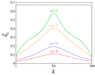
Figure 1: Normalized participation ratio of eigenstates $\xi_{k}$ for different values of $\alpha$ for a uniform channel ($J_{i,j}=J$) composed of $N=100$ spins with on-site disorder given by Eq. (3). Each curve was obtained by exact numerical diagonalization of Eq. (1) and further averaging $\xi_{k}$ over $10^{3}$ independent realizations of disorder. Note that $\xi_{k}$ goes from $0.01$ for completely localized states to $1$ for uniformely extended states. For comparison, the dashed curve above (constant at $2/3$) shows the participation ratio distribution for the harmonic eigenstates of the noiseless case. Here we clearly see that the presence of long-range correlations in the disorder distribution promotes the appearance of delocalized states around the middle of the band

Figure 1 shows the resulting $\xi_{k}$ distribution (averaged over $10^{3}$ independent samples) as the degree of long-range correlations $\alpha$ is increased for a on-site-disordered channel consisting of $N=100$ spins, including the noiseless case ($\omega_{n}\rightarrow 0$) for comparison (dashed line). Note that we are considering the channel Hamiltonian only [cf. Eq. (1)], with $g_{\nu}=0$. Indeed, a prominent set of delocalized eigenstates builds up around the band center. First of all, we should remark that the slight deflection of the $\alpha=0$ curve (uncorrelated disorder) is solely due to the well known fact that the states at the band edges are more localized than those near the band center. This gets much more pronounced when $\alpha=2$ and higher, as expected. Indeed, $\alpha>2$ sets the transition point from an insulator to a metallic phase in eletronic tight-binding models, characterized by vanishing Lyapunov coefficients in the central part of the spectrum de Moura and Lyra (1998). This happens exactly when the sequences generated by Eq. (3) display persistent increments according to the Hurst classification scheme Feder (1988).

The likelihood of delocalized states in the presence of substantial amounts of disorder, not to mention the lack of mirror symmetry due to the on-site magnetic field distribution across the chain, sounds quite appealing. It means there is a suitable region in the frequency band of the channel – in our case, in the middle of it, as seen in Fig. 1 – to tune the sender and receiver spins with. The corresponding eigenstates, featuring a delocalized nature, will display a broader amplitude distribution with greater balance between $a_{rk}$ and $a_{sk}$ thereby increasing the chances of inducing a small detuning $\Delta$ [cf. Eqs. (8), (9), and (10)], which is crucial for having very high transfer fidelities. Figure 2 shows how the absolute value of the ratio $\Delta/J^{\prime}$ (averaged over several samples) behaves with $\alpha$ thus leaving no doubt the onset of long-range correlations establishes a suitable ground for carrying out quantum communication protocols with weakly-coupled parties. As discussed earlier, uncorrelated fluctuations ($\alpha=0$) rules out any possibility of doing so, the ratio being extremely high. Things then get rapidly improved with $\alpha$ suggesting that already for $\alpha>2$ one should obtain satisfying outcomes in the QST protocol, as we show in the following section.

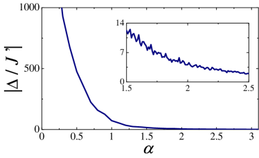
Figure 2: (Color online) Absolute value of detuning $\Delta=h_{s}-h_{r}$ in units of $J^{\prime}$ versus $\alpha$ averaged over $500$ independent realizations of disorder for a channel featuring $N=50$ spins with $\omega_{\nu}=0$. Results were obtained from exact numerical diagonalization of Hamiltonian (1). Naturally, we are assuming very small outer couplings $g_{\nu}$ so that the effective description, Eq. (8), holds. The inset shows the very same quantity, zoomed in into the $\alpha=1.5$ to $\alpha=2.5$ interval.

V Quantum-state transfer protocol

The standard QST protocol goes as follows Bose (2003). Suppose that Alice is able to control the spin located at position $s$ and wants to send an arbitrary qubit $|\phi\rangle_{s}=\alpha|\downarrow\rangle_{s}+\beta|\uparrow\rangle_{s}$ to Bob which has access to spin $r$. Now let us assume that the rest of the chain is initialized in the fully polarized spin-down state so that the whole state reads $|\Psi(0)\rangle=|\phi\rangle_{s}|\downarrow\rangle_{1}\ldots|\downarrow\rangle_{N}|\downarrow\rangle_{r}$. She then let the system evolve following its natural dynamics, $|\psi(t)\rangle=\hat{\mathcal{U}}(t)|\psi(0)\rangle$, where $\hat{\mathcal{U}}(t)\equiv e^{-i\hat{H}t}$ is the unitary time-evolution operator. Ideally, she expects that at some prescribed time $\tau$ the evolved state takes the form $|\Psi(\tau)\rangle=|\downarrow\rangle_{s}|\downarrow\rangle_{1}\ldots|\downarrow\rangle_{N}|\phi\rangle_{r}$. At this point, Bob receives state $\rho_{r}(\tau)=\mathrm{Tr}_{s,1,\ldots,N}|\Psi(\tau)\rangle\langle\Psi(\tau)|$ and thus the transfer fidelity can be evaluated by $F_{\phi}(\tau)=\langle\phi|\rho_{r}(\tau)|\phi\rangle$ Note, however, that this measures the performance of QST for a specific input. In order to properly evaluate the efficiency of the channel, we may average the above quantity over all input states $|\phi\rangle_{s}$ (that is, over the Bloch sphere) which results in Bose (2003)

$$F(t)=\dfrac{1}{2}+\dfrac{f_{r}(t)}{3}+\dfrac{f_{r}(t)^{2}}{6}$$ (12)

for an arbitrary time with $f_{i}(t)\equiv|\langle i|e^{-i\hat{H}t}|s\rangle|$ Therefore, we note that such a state-independent figure of merit of QST depends solely upon the transition amplitude between the sender and receiver spins with $F(t)=1$ only when $f_{r}(t)=1$. The problem of transmitting a qubit state from one point to another can thus be viewed as a single-particle continuous quantum walk Kempe (2003) on a network and the goal is to find out ways to transfer the excitation between two distant nodes with the highest possible transition amplitude.

In the case of weakly-coupled spins in which an effective two-site interaction sets in [cf. Eq. (8)], the transition amplitude $f_{r}(t)$ will strongly depend upon the resonance between $h_{s}$ and $h_{r}$, that is $\Delta$. In the previous section, we have seen that the emergence of long-range correlations (see Fig. 2) favors smaller values of $\Delta$. Now, let us finally see about the resulting QST performance. As a testbed, we consider a $N=50$ channel, $g_{\nu}=g=0.001$ (in units of $J$), and $\omega_{\nu}=0$. Given the size of the channel, this chosen value for $g$ assures that the subspace created by states $|s\rangle$ and $|r\rangle$ becomes safely shielded from influence of channel normal modes lying around the band center. Even if one of them gets close by, it is very likely that the eigenstate will not be extremely asymmetric due to the presence of delocalized states for high enough $\alpha$ [see Fig. 1].

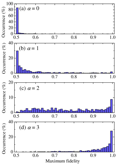
Figure 3: (Color online) Maximum-fidelity histogram for 500 indepedent realizations of disorder for $\alpha=0,1,2,$ and $3$. Results were obtained from exact numerical diagonalization of the full Hamiltonian $\hat{H}=\hat{H}_{\mathrm{ch}}+\hat{H}_{\mathrm{int}}$ with $N=50$, $\omega_{n}$, $n=1,\ldots,N$, given by Eq. (3), $\omega_{\nu}=0$, $g_{\nu}=g=0.001$ (in units of $J$). The maximum fidelity $F_{\mathrm{max}}=\mathrm{max}\{F(t)\}$ [see Eq. (12)] was registered during time interval $[0,20\tau]$, with $\tau=\pi/(2g^{2})$.

In Fig. 3 we show the sample distribution of the maximum fidelity $F_{\mathrm{max}}=\mathrm{max}\{F(t)\}$ [as defined above in Eq. (12)] achieved in time interval $t\in[0,20\tau]$, with $\tau=\pi/(2g^{2})$ being the corresponding time (in units of $1/J$) for which a complete transfer would occur for the noiseless case, $f_{r}(\tau)\approx 1$, as seen in Sec. III. That interval is a pretty reasonable one in order to guarantee at least one full Rabi cycle in most of the samples. Recall that the effective sender-receiver hopping strength $J^{\prime}$ dictates the time scale of the dynamics and is strongly affected by disorder. Figure 3 ultimately confirms what it has been suggested by Fig. 2. Indeed, strong long-range correlations in the disorder distribution enhances the figure of merit of QST enormously. Even more impressive is the fact that, for $\alpha=2$ and $\alpha=3$ [see Figs. 3(c) and 3(d), respectively], we find the number of occurrences of fidelities $F_{\mathrm{max}}\approx 1$ to be the highest one. We also note that the fidelities for $\alpha=2$ case [Fig. 3(c)] is fairly well distributed across all the possible outcomes, thus indicating a transition regime.

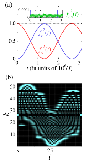
Figure 4: (Color online) (a) Time evolution of the occupation probability amplitudes for the sender $f_{s}^{2}(t)$, receiver $f_{r}^{2}(t)$, and channel spins, the latter being the sum of the amplitudes within the channel, namely $f_{\mathrm{ch}}^{2}(t)\equiv\sum_{n=1}^{N}f_{n}^{2}(t)$. For this particular realization, we simply took one of the samples which provided $F_{\mathrm{max}}\approx 1$ in Fig. 3(d) for $\alpha=3$. Note that the time scale has been reduced to twice the transfer time for the noiseless case, that is $2\tau$, for a better view of a Rabi-like cycle. The inset shows the very same graph but for a much smaller scale of amplitude in order to account for the (rather negligible) behavior of $f_{\mathrm{ch}}^{2}(t)$. (b) Corresponding density plot of the eigenstate spatial distribution $|\langle|i|\psi_{k}\rangle|^{2}$ for every $k$ (in increasing order of energy). Darker (brighter) spots indicate lower (higher) overlaps. Note the formation of a pair of states in the middle of the band with strong overlap in $|s\rangle$ and $|r\rangle$ simultaneously. These are the source of such high-fidelity QST rounds.

In order to provide an explicit view on what is actually going on in the QST process, in Fig. 4(a) we show the time evolution of the occupation probabilities $f_{i}^{2}(t)$ of the sender ($i=s$), receiver ($i=r$), and channel [$f_{\mathrm{ch}}^{2}(t)\equiv\sum_{n=1}^{N}f_{n}^{2}(t)$] spins for one particular (ordinary) sample, out of many successful ones (meaning $F_{\mathrm{max}}\approx 1$) encountered for $\alpha=3$ [see Fig. 3(d)]. There we see a genuine Rabi-like behavior yielding a very high-quality QST. We reduced the time scale to $2\tau$ so we can have a more detailed view on a complete cycle. Therefore, in this case the transfer time happens to be roughly the same as for the noiseless case. Further, we note that the channel is barely populated for all practical purposes [see the inset of Fig 4(a)], meaning that Eq. (8) is a robust approximation. Those residual beatings seen for $f_{\mathrm{ch}}^{2}(t)$ in are due to some negligible mixing between both channel and sender/receiver subspaces. One could get rid of it by further decreasing $g$. Care must taken, though, not to compromise the transfer time scale since it increases $\propto\ 1/g^{2}$.

Figure 4(b) shows the corresponding spatial distribution of eigenstates, $|\langle|i|\psi_{k}\rangle|^{2}$, along the whole spectrum $k$. First, note that the outer parts of the spectrum are mostly populated by localized-like eigenstates. Indeed, the eigenstates get more delocalized as we move towards the center of the band, as discussed before [see Fig. 1]. We also point out the asymmetrical aspect of the eigenstate distribution. Still, it turns out to be possible to span an independent subspace involving only the sender and receiver spins [Eq. 8] so that their corresponding eigenstates become close to $|s\rangle\pm|r\rangle)/\sqrt{2}$. By looking closely at Fig 4(b), we also spot a few eigenstates showing strong asymmetries between spins $1$ and $N$. Fortunately, since $a_{sk}$ and $a_{rk}$ is fairly balanced across the spectrum and due to the fact that the channel eigenstates lying around the middle of the band (less asymmetric) have great influence on $\Delta/J^{\prime}$, given that the terms in the sum in Eqs. (9) and (10) goes $\sim 1/E_{k}$, the sender and receiver spins are able to find a way out through such asymmetries and establish an effective resonant interaction between them thus resulting in an almost perfect QST for most of the samples.

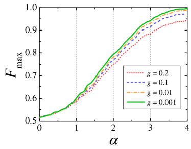
Figure 5: (Color online) Maximum fidelity versus $\alpha$ averaged over 500 independent disorder realizations. Now, we have set $g=0.001$, $0.01$, $0.1$, and $0.2$ (in units of $J$) while other system’s parameters were kept as usual, namely $N=50$ and $\omega_{\nu}=0$. The maximum fidelity $F_{\mathrm{max}}=\mathrm{max}\{F(t)\}$ for each sample was again obtained during time interval $[0,20\tau]$, with $\tau=\pi/(2g^{2})$.

Last, in order to evaluate a representative outcome for $F_{\mathrm{max}}$ for a given $\alpha$, in Fig 5 we plot its average over all the samples for a large window of $\alpha$ values. This clearly illustrates the overall behavior of the occurrences of $F_{\mathrm{max}}$ as one increases the degree of long-range correlations in the disorder distribution. Note that we are also showing the curve for many values of $g$, only to stress the importance of setting this parameter as smaller as possible so as to avoid mixing between the channel and sender/receiver subspaces. Indeed, we see quality of QST is affected by that. As we go towards smaller values of $g$, there is a saturation point indicating that Hamiltonian 8 has reached its final form. It means that if we keep on decreasing $g$, the QST fidelity will not get any better and the time scale of the transfer will increase substantially. Finally, we identify in Fig. 5 that the $F_{\mathrm{max}}$ growth profile is more pronounced between $\alpha=1$ and $\alpha=3$ until it saturates for higher values of $\alpha$. This is associated to the fact that the long-range correlated sequence generate by Eq. (3) becomes nonstationary for $\alpha>1$ and acquires persistent character when $\alpha>2$, thereby triggering the appearance of delocalized states in the middle of the band de Moura and Lyra (1998); Domínguez-Adame et al. (2003).

VI Concluding remarks

We studied a QST protocol through a $XX$ spin channel with on-site long-range-correlated disorder. The protocol involved a couple of communicating spins weakly coupled to the channel not matching with any of its normal modes so that the transfer takes place through Rabi-like oscillations between the ends of the chain Wójcik et al. (2005); Almeida et al. (2016). We focused on the reduced sender/receiver description based on Hamiltonian (8) which embodies all the relevant information regarding the way they are affected by the channel, thus allowing one to foresee the QST outcome based on the renormalized parameters contained in the two-site effective Hamiltonian.

We showed that this class of weakly-coupled models are indeed robust against external perturbations Yao et al. (2011) as the effective interaction between sender and receiver spins do not depend upon the entire wavefunction of the spectrum but rather on the local amplitudes of the spins they are connected to. Because of that, we realize we do not necessarily need a perfect symmetric chain to to achieve an almost perfect QST. When scale-free correlations with a power-law spectral density $S(k)\propto k^{-\alpha}$ set in, the disorder distribution is such that it can support delocalized eigenstates around the center of the band de Moura and Lyra (1998). Those are able to provide a broader, more balanced distribution of amplitudes even in the presence of asymmetries, what makes it possible to induce effective resonant interactions between $|r\rangle$ and $|s\rangle$, provided $\alpha$ is high enough, thus resulting in extremely high fidelities, with most of the samples providing $F_{\mathrm{max}}\approx 1$.

Note that we have not considered the case of structural disorder here, that is, fluctuations on the spin couplings. However, on-site disorder actually embodies a worst-case, and hence more realistic, scenario since the spectrum also looses its symmetry, differently from structural fluctuations.

We remark that disorder, either correlated or not, might arise naturally due to experimental imperfections in the manufacturing process of solid state devices for quantum information processing. However, we may also think about inducing those correlations somehow since, as we have shown, it may not be so detrimental for certain communication tasks as in the uncorrelated-disorder scenario. Overall, it should be easier to allow for that than designing a chain with a very specific set of parameters, which demands a high degree of control. Our work further promotes the study of quantum communication protocols in disordered, asymmetric, spin chains.

VII Acknowledgments

This work was partially supported by CNPq (Grant No. 152722/2016-5), CAPES, FINEP, and FAPEAL (Brazilian agencies).

References

- Cirac et al. (1997) J. I. Cirac, P. Zoller, H. J. Kimble, and H. Mabuchi, Phys. Rev. Lett. 78, 3221 (1997).
- Kimble (2008) H. J. Kimble, Nature 453, 1023 (2008).
- Bose (2003) S. Bose, Phys. Rev. Lett. 91, 207901 (2003).
- Christandl et al. (2004) M. Christandl, N. Datta, A. Ekert, and A. J. Landahl, Phys. Rev. Lett. 92, 187902 (2004).
- Plenio et al. (2004) M. B. Plenio, J. Hartley, and J. Eisert, New Journal of Physics 6, 36 (2004).
- Osborne and Linden (2004) T. J. Osborne and N. Linden, Phys. Rev. A 69, 052315 (2004).
- Wójcik et al. (2005) A. Wójcik, T. Łuczak, P. Kurzyński, A. Grudka, T. Gdala, and M. Bednarska, Phys. Rev. A 72, 034303 (2005).
- Wójcik et al. (2007) A. Wójcik, T. Łuczak, P. Kurzyński, A. Grudka, T. Gdala, and M. Bednarska, Phys. Rev. A 75, 022330 (2007).
- Li et al. (2005) Y. Li, T. Shi, B. Chen, Z. Song, and C.-P. Sun, Phys. Rev. A 71, 022301 (2005).
- Huo et al. (2008) M. X. Huo, Y. Li, Z. Song, and C. P. Sun, Europhysics Letters 84, 30004 (2008).
- Gualdi et al. (2008) G. Gualdi, V. Kostak, I. Marzoli, and P. Tombesi, Phys. Rev. A 78, 022325 (2008).
- Banchi et al. (2010) L. Banchi, T. J. G. Apollaro, A. Cuccoli, R. Vaia, and P. Verrucchi, Phys. Rev. A 82, 052321 (2010).
- Banchi et al. (2011) L. Banchi, T. J. G. Apollaro, A. Cuccoli, R. Vaia, and P. Verrucchi, New Journal of Physics 13, 123006 (2011).
- Apollaro et al. (2012) T. J. G. Apollaro, L. Banchi, A. Cuccoli, R. Vaia, and P. Verrucchi, Phys. Rev. A 85, 052319 (2012).
- Lorenzo et al. (2013) S. Lorenzo, T. J. G. Apollaro, A. Sindona, and F. Plastina, Phys. Rev. A 87, 042313 (2013).
- Lorenzo et al. (2015) S. Lorenzo, T. J. G. Apollaro, S. Paganelli, G. M. Palma, and F. Plastina, Phys. Rev. A 91, 042321 (2015).
- Almeida et al. (2016) G. M. A. Almeida, F. Ciccarello, T. J. G. Apollaro, and A. M. C. Souza, Phys. Rev. A 93, 032310 (2016).
- Amico et al. (2004) L. Amico, A. Osterloh, F. Plastina, R. Fazio, and G. Massimo Palma, Phys. Rev. A 69, 022304 (2004).
- Plenio and Semião (2005) M. B. Plenio and F. L. Semião, New Journal of Physics 7, 73 (2005).
- Apollaro and Plastina (2006) T. J. G. Apollaro and F. Plastina, Phys. Rev. A 74, 062316 (2006).
- Plastina and Apollaro (2007) F. Plastina and T. J. G. Apollaro, Phys. Rev. Lett. 99, 177210 (2007).
- Apollaro et al. (2008) T. J. Apollaro, A. Cuccoli, A. Fubini, F. Plastina, and P. Verrucchi, Phys. Rev. A 77, 062314 (2008).
- Campos Venuti et al. (2007) L. Campos Venuti, S. M. Giampaolo, F. Illuminati, and P. Zanardi, Phys. Rev. A 76, 052328 (2007).
- Cubitt and Cirac (2008) T. S. Cubitt and J. I. Cirac, Phys. Rev. Lett. 100, 180406 (2008).
- Giampaolo and Illuminati (2009) S. M. Giampaolo and F. Illuminati, Phys. Rev. A 80, 050301 (2009).
- Giampaolo and Illuminati (2010) S. M. Giampaolo and F. Illuminati, New Journal of Physics 12, 025019 (2010).
- Gualdi et al. (2011) G. Gualdi, S. M. Giampaolo, and F. Illuminati, Phys. Rev. Lett. 106, 050501 (2011).
- Estarellas et al. (2017a) M. P. Estarellas, I. D’Amico, and T. P. Spiller, Phys. Rev. A 95, 042335 (2017a).
- Estarellas et al. (2017b) M. P. Estarellas, I. D’Amico, and T. P. Spiller, Scientific Reports 7, 42904 (2017b).
- Almeida et al. (2017) G. M. A. Almeida, F. A. B. F. de Moura, T. J. G. Apollaro, and M. L. Lyra, arXiv:1707.05865 [quant-ph] (2017).
- Feder (2006) D. L. Feder, Phys. Rev. Lett. 97, 180502 (2006).
- De Chiara et al. (2005) G. De Chiara, D. Rossini, S. Montangero, and R. Fazio, Phys. Rev. A 72, 012323 (2005).
- Zwick et al. (2011) A. Zwick, G. A. Álvarez, J. Stolze, and O. Osenda, Phys. Rev. A 84, 022311 (2011).
- Zwick et al. (2012) A. Zwick, G. A. Álvarez, J. Stolze, and O. Osenda, Phys. Rev. A 85, 012318 (2012).
- Paganelli et al. (2013) S. Paganelli, S. Lorenzo, T. J. G. Apollaro, F. Plastina, and G. L. Giorgi, Phys. Rev. A 87, 062309 (2013).
- Fitzsimons and Twamley (2005) J. Fitzsimons and J. Twamley, Phys. Rev. A 72, 050301 (2005).
- Burgarth and Bose (2005) D. Burgarth and S. Bose, New Journal of Physics 7, 135 (2005).
- Tsomokos et al. (2007) D. I. Tsomokos, M. J. Hartmann, S. F. Huelga, and M. B. Plenio, New Journal of Physics 9, 79 (2007).
- Petrosyan et al. (2010) D. Petrosyan, G. M. Nikolopoulos, and P. Lambropoulos, Phys. Rev. A 81, 042307 (2010).
- Yao et al. (2011) N. Y. Yao, L. Jiang, A. V. Gorshkov, Z.-X. Gong, A. Zhai, L.-M. Duan, and M. D. Lukin, Phys. Rev. Lett. 106, 040505 (2011).
- Bruderer et al. (2012) M. Bruderer, K. Franke, S. Ragg, W. Belzig, and D. Obreschkow, Phys. Rev. A 85, 022312 (2012).
- Kay (2016) A. Kay, Phys. Rev. A 93, 042320 (2016).
- Anderson (1958) P. W. Anderson, Phys. Rev. 109, 1492 (1958).
- Abrahams et al. (1979) E. Abrahams, P. W. Anderson, D. C. Licciardello, and T. V. Ramakrishnan, Phys. Rev. Lett. 42, 673 (1979).
- Albanese et al. (2004) C. Albanese, M. Christandl, N. Datta, and A. Ekert, Phys. Rev. Lett. 93, 230502 (2004).
- Flores (1989) J. C. Flores, Journal of Physics: Condensed Matter 1, 8471 (1989).
- Dunlap et al. (1990) D. H. Dunlap, H.-L. Wu, and P. W. Phillips, Phys. Rev. Lett. 65, 88 (1990).
- Phillips and Wu (1991) P. Phillips and H.-L. Wu, Science 252, 1805 (1991).
- de Moura and Lyra (1998) F. A. B. F. de Moura and M. L. Lyra, Phys. Rev. Lett. 81, 3735 (1998).
- Izrailev and Krokhin (1999) F. M. Izrailev and A. A. Krokhin, Phys. Rev. Lett. 82, 4062 (1999).
- Kuhl et al. (2000) U. Kuhl, F. M. Izrailev, A. A. Krokhin, and H.-J. Stöckmann, Applied Physics Letters 77, 633 (2000).
- Lima et al. (2002) R. P. A. Lima, M. L. Lyra, E. M. Nascimento, and A. D. de Jesus, Phys. Rev. B 65, 104416 (2002).
- de Moura et al. (2002) F. A. B. F. de Moura, M. D. Coutinho-Filho, E. P. Raposo, and M. L. Lyra, Phys. Rev. B 66, 014418 (2002).
- Nunes et al. (2016) D. Nunes, A. R. Neto, and F. de Moura, Journal of Magnetism and Magnetic Materials 410, 165 (2016).
- de Moura et al. (2003) F. A. B. F. de Moura, M. D. Coutinho-Filho, E. P. Raposo, and M. L. Lyra, Phys. Rev. B 68, 012202 (2003).
- Domínguez-Adame et al. (2003) F. Domínguez-Adame, V. A. Malyshev, F. A. B. F. de Moura, and M. L. Lyra, Phys. Rev. Lett. 91, 197402 (2003).
- Herrera-González et al. (2014) I. F. Herrera-González, J. A. Méndez-Bermúdez, and F. M. Izrailev, Phys. Rev. E 90, 042115 (2014).
- Lam and Sander (1992) C.-H. Lam and L. M. Sander, Phys. Rev. Lett. 69, 3338 (1992).
- Peng et al. (1992) C.-K. Peng, S. V. Buldyrev, A. L. Goldberger, S. Havlin, F. Sciortino, M. Simons, and H. E. Stanley, Nature 356, 168 (1992).
- Carreras et al. (1998) B. A. Carreras, B. van Milligen, M. A. Pedrosa, R. Balbín, C. Hidalgo, D. E. Newman, E. Sánchez, M. Frances, I. García-Cortés, J. Bleuel, M. Endler, S. Davies, and G. F. Matthews, Phys. Rev. Lett. 80, 4438 (1998).
- Carpena et al. (2002) P. Carpena, P. Bernaola-Galvan, P. C. Ivanov, and H. E. Stanley, Nature 418, 955 (2002).
- Feder (1988) J. Feder, Fractals (Plenum Press, New York, 1988).
- Paczuski et al. (1996) M. Paczuski, S. Maslov, and P. Bak, Phys. Rev. E 53, 414 (1996).
- Ciccarello (2011) F. Ciccarello, Phys. Rev. A 83, 043802 (2011).
- Thouless (1974) D. J. Thouless, Physics Reports 13, 93 (1974).
- Kempe (2003) J. Kempe, Contemporary Physics 44, 307 (2003).