Percolation thresholds and fractal dimensions for square and cubic lattices with long-range correlated defects

Abstract

We study long-range power-law correlated disorder on square and cubic lattices. In particular, we present high-precision results for the percolation thresholds and the fractal dimension of the largest clusters as function of the correlation strength. The correlations are generated using a discrete version of the Fourier filtering method. We consider two different metrics to set the length scales over which the correlations decay, showing that the percolation thresholds are highly sensitive to such system details. By contrast, we verify that the fractal dimension $d_{\rm f}$ is a universal quantity and unaffected by the choice of metric. We also show that for weak correlations, its value coincides with that for the uncorrelated system. In two dimensions we observe a clear increase of the fractal dimension with increasing correlation strength, approaching $d_{\rm f}\rightarrow 2$. The onset of this change does not seem to be determined by the extended Harris criterion.

I Introduction

Structural obstacles (impurities) play an important role for a wide range of physical processes as most substrates and surfaces in nature are rough and inhomogeneous Pfeifer and Avnir (1983); Avnir et al. (1984). For example, the properties of magnetic crystals are often altered by the presence of extended defects in the form of linear dislocations or regions of different phases Dorogovtsev (1980); Yamazaki et al. (1986). Another important class of such disordered media are porous materials, which often exhibit large spatial inhomogeneities of a fractal nature. Such fractal disorder affects a medium’s conductivity, and diffusive transport can become anomalous Bouchaud and Georges (1990); Malek and Coppens (2001); Foulaadvand and Sadrara (2015); Goychuk et al. (2017). This aspect is relevant, for instance, for the recovery of oil through porous rocks Dullien (1979); Sahimi (1995), for the dynamics of fluids in disordered media Skinner et al. (2013); Spanner et al. (2016), or for our understanding of transport processes in biological cells Bancaud et al. (2012); Höfling and Franosch (2013).

Disordered systems are conveniently studied in the framework of lattice models with randomly positioned defects (or empty sites). Of particular interest is the situation where the concentration of occupied (i.e., non-defect) lattice sites is near the percolation threshold and clusters of connected occupied sites become fractal. The case where defects are uncorrelated is a classic textbook model, whose properties have been studied extensively Stauffer and Aharony (1992). In nature, however, inhomogeneities are often not distributed completely at random but tend to be correlated over large distances. To understand the impact of this, it is useful to consider the limiting case where correlations asymptotically decay by a power law rather than exponentially with distance:

$$C({\bf r})\sim|{\bf r}|^{-a}.$$ (1)

An illustration of such power-law correlations for continuous and discrete site variables on a square lattice is shown in Fig. 1. If the correlation parameter $a$ is smaller than the spatial dimension $D$, the correlations are considered long-range or “infinite”.

The problem of power-law correlated disorder has first been investigated in the context of spin systems and later for percolation Weinrib and Halperin (1983); Weinrib (1984). The relevance of the disorder was shown to be characterized by an extension of the Harris criterion for uncorrelated defects Harris (1974): the critical behavior of the system deviates from the uncorrelated case if the minimum of $D$ and $a$ is smaller than $2/\nu$ (where $\nu$ denotes the correlation-length exponent for the ordered system). It was furthermore argued that in the regime of strong correlations, the critical correlation-length exponent for strong disorder is universally given by $2/a$. Since $D$ is always larger than $2/\nu$ for percolation, the correlation-length exponent for long-range correlated percolation is given by

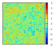
Figure 1: Illustration of long-range correlated defects on a $2048^{2}$ lattice with correlation parameter $a=0.5$. (left) Continuous correlated Gaussian random variables. The color reflects the value at the respective lattice site. (right) Corresponding lattice of discrete variables at the finite-size percolation threshold $p_{c}^{L}=0.522$ with defects shown in black.

$$\nu_{a}=\begin{cases}2/a\quad&\text{for }a<a_{\rm H}=2/\nu\\ \nu\quad&\text{for }a\geq a_{\rm H}=2/\nu.\\ \end{cases}$$ (2)

The extended Harris criterion is still slightly controversial Prudnikov and Fedorenko (1999); Prudnikov et al. (2000), but it has to some extent been supported by numerical investigations Schrenk et al. (2013); Prakash et al. (1992); Makse et al. (1998). These studies made use of the Fourier filtering method (FFM) Saupe (1988); Peng et al. (1991); Prakash et al. (1992); Makse et al. (1995a, 1998); Pang et al. (1995); Makse et al. (1996); Ballesteros and Parisi (1999); Ahrens and Hartmann (2011); Simon et al. (2012); Schrenk et al. (2013) to generate power-law correlated disorder and have yielded estimates for critical exponents and fractal dimensions characterizing the system in $2D$. However, they in part used semi-analytical implementations of the FFM, involving various approximations and free parameters. In this work we use a numerical version without free parameters, and whose errors are fully controlled.

The remainder of the article is organized as follows: Section II gives a detailed description of the FFM, so that our implementation is easily reproducible . Thereafter, in Sec. III, we specify how the mapping to discrete site variables is carried out. In the following Sec. IV, we present our results for the percolation thresholds on square and cubic lattices. Our main findings, regarding the fractal dimension $d_{\rm f}$ for long-range correlated percolation clusters in $2D$ and $3D$, are discussed in Sec. V. Finally, our results and conclusions are summarized in Sec. VI.

II Generating long-range correlated disorder

We start with the more general problem of how to obtain a hyper-cubic lattice $L^{D}$ of identically distributed random variables $\tau_{{\bf x}}\in\mathbb{R}$ that exhibit correlations of the form

$$\left\langle\tau_{{\bf x}}\tau_{{\bf x}+{\bf r}}\right\rangle=C_{{\bf r}},$$ (3)

where $\left\langle\ldots\right\rangle$ denotes the expectation value and $C_{\bf r}$ is a (discrete) correlation function. $C_{{\bf r}}$ should be symmetric around zero and periodic along all spatial dimensions, i.e., $C_{{\bf r}+L{\bf e}_{i}}=C_{{\bf r}}$ for all unit vectors ${\bf e}_{1},\ldots,{\bf e}_{D}$. It is furthermore convenient to choose $\tau_{{\bf x}}$ as Gaussian random variables with mean $\left\langle\tau_{{\bf x}}\right\rangle=\left\langle\tau\right\rangle=0$ and variance $\sigma^{2}_{\tau}=1$. Otherwise, we consider $C_{{\bf r}}$ to be an arbitrary function for now. (Note that we use the index notation for explicitly discrete functions).

We use a variant of the Fourier filtering method that employs discrete Fourier transforms (DFT) and is similar to that from Ref. Ahrens and Hartmann (2011); Simon et al. (2012). The key idea of the FFM is to correlate random variables in Fourier space. The result of the inverse transform will in general be complex numbers, $\varphi_{{\bf x}}=\varphi^{\rm re}_{{\bf x}}+i\varphi^{\rm im}_{{\bf x}}$. To explain how the method works, let us now assume that we already have a lattice of complex random variables $\varphi_{{\bf x}}$. Let us further assume that $\{\varphi^{\rm re}_{{\bf x}}\}$ and $\{\varphi^{\rm im}_{{\bf x}}\}$ are independent sets of random variables, each spatially correlated according to Eq. (3), i.e.,

$$\left\langle\varphi^{\rm re}_{{\bf x}}\varphi^{\rm re}_{{\bf x}+{\bf r}}\right\rangle =\left\langle\varphi^{\rm im}_{{\bf x}}\varphi^{\rm im}_{{\bf x}+{\bf r}}\right\rangle=C_{{\bf r}},$$

$$\left\langle\varphi^{\rm re}_{{\bf x}}\varphi^{\rm im}_{{\bf x}+{\bf r}}\right\rangle =\left\langle\varphi^{\rm im}_{{\bf x}}\varphi^{\rm re}_{{\bf x}+{\bf r}}\right\rangle=0,$$ (4)

and see what that implies for the distributions of Fourier coefficients.

As we are interested in a discrete lattice with periodic boundary conditions of linear size $L$ and volume $N=L^{D}$, we consider a DFT of the form

$$\varPhi_{{\bf k}} =\phantom{\frac{1}{N}}\sum_{{\bf x}}\varphi_{{\bf x}}e^{\frac{2\pi i{\bf k}{\bf x}}{L}},$$ (5)

$$\varphi_{{\bf x}} =\frac{1}{N}\sum_{{\bf k}}\varPhi_{{\bf k}}e^{-\frac{2\pi i{\bf k}{\bf x}}{L}},$$ (6)

where $\sum_{{\bf x}}$ denotes the $D$-dimensional sum over possible realizations of the vector ${\bf x}$ on the hypercubic lattice. In practice, we employ a numerical fast Fourier transform (FFT) Press et al. (2007) and follow the convention that $x_{i}\in[0,L)$ and $k_{i}\in[0,L)$.

As shown in Appendix A, the correlation function is connected to the Fourier coefficients via

$$2C_{{\bf r}}=\left\langle\varphi_{{\bf x}}^{*}\varphi_{{\bf x}+{\bf r}}^{\phantom{*}}\right\rangle=\frac{1}{N^{2}}\sum_{\bf k}\left\langle|\varPhi_{{\bf k}}|^{2}\right\rangle e^{-\frac{2\pi i{\bf k}{\bf r}}{L}}.$$ (7)

The discrete spectral density

$$S_{\bf k}=\sum_{\bf r}C_{{\bf r}}e^{\frac{2\pi i{\bf k}{\bf r}}{L}}$$ (8)

can thus be written as

$$S_{\bf k} =\sum_{\bf r}\frac{1}{2N^{2}}\sum_{{\bf k}^{\prime}}\left\langle|\varPhi_{{\bf k}^{\prime}}|^{2}\right\rangle e^{-\frac{2\pi i{\bf k}^{\prime}{\bf r}}{L}}e^{\frac{2\pi i{\bf k}{\bf r}}{L}}$$

$$=\frac{1}{2N}\sum_{{\bf k}^{\prime}}\left\langle|\varPhi_{{\bf k}^{\prime}}|^{2}\right\rangle\delta_{{\bf k}^{\prime},{\bf k}}=\frac{1}{2N}\left\langle|\varPhi_{{\bf k}}|^{2}\right\rangle$$

$$=\frac{1}{2N}\left(\left\langle{\varPhi^{\rm re}_{{\bf k}}}^{2}\right\rangle+\left\langle{\varPhi^{\rm im}_{{\bf k}}}^{2}\right\rangle\right).$$ (9)

In return, this means we can generate complex real-space random variables with the desired correlation from Fourier-space random variables that satisfy Eq. (9). It is convenient to consider distributions of $\varPhi_{{\bf k}}$ with zero mean, so that Eq. (9) can be expressed in terms of the variance:

$$2NS_{\bf k}=\sigma^{2}_{\varPhi_{{\bf k}}}=\sigma^{2}_{\varPhi^{\rm re}_{{\bf k}}}+\sigma^{2}_{\varPhi^{\rm im}_{{\bf k}}}.$$ (10)

Hence, we can simply draw real and imaginary parts of $\varPhi_{{\bf k}}$ independently from identical distributions (for each frequency ${\bf k}$):

$$\varPhi^{\rm re/im}_{{\bf k}}=\sqrt{S_{\bf k}}U,$$ (11)

where $U$ is a random variable with mean $\left\langle U\right\rangle=0$ and variance $\sigma^{2}_{U}=N$. Transforming $\varPhi_{{\bf k}}$ back to ${\bf x}$-space, we get two sets of variables, $\{\varphi^{\rm re}_{{\bf x}}\}$ and $\{\varphi^{\rm im}_{{\bf x}}\}$, each with zero mean and spatial correlations $C_{{\bf r}}$. Thanks to the orthogonality of the Fourier transform, the two sets are statistically independent. Each can be associated with the real random site variables $\tau_{{\bf x}}$ in Eq. (3) and used for further analysis. We draw $U$ from a Gaussian distribution, and so the resulting distributions will also be Gaussian. (In fact, they would be Gaussian anyway for large systems due to the central limit theorem.)

The derivation above did not use any assumptions regarding the correlation function $C_{{\bf r}}$. However, we see from Eq. (9) that its Fourier transform $S_{{\bf k}}$ needs to be positive. Any $C_{{\bf r}}$ that is symmetric (around zero) will give rise to real $S_{\bf k}$, but the positivity constraint is somewhat problematic. For the continuum Fourier transform, it is in fact also implied by the symmetry Makse et al. (1996), but for discrete systems, some values of $S_{\bf k}$ can become negative. This has to do with the restricted frequency range, leading to an aliasing effect that causes periodic modulations on the signal. Note, however, that this is not just an artifact of the method, but rather implies that some correlations are fundamentally not possible on a finite discrete lattice. In practice, we can simply fix this problem by setting all negative values of $S_{{\bf k}}$ to zero (“zero-cutoff”). While this will inevitably modify the resulting correlations, the effect is usually negligible and vanishes rapidly with increasing system size, see Appendix B.

In short, our version of the FFM can be summarized as follows:

1. Choose a discrete correlation function $C_{\bf r}$ that is symmetric around zero. For optimal performance, the linear size of the lattice should be $L=2^{l}$ with integer $l$.

2. Perform a DFT, $C_{{\bf r}}\rightarrow S_{{\bf k}}$, and set $S_{{\bf k}}=0$ for all $S_{{\bf k}}<0$ (zero-cutoff). This step only needs to be done once for the whole disorder ensemble.

3. Construct real and imaginary parts of each component independently, $\varPhi^{\rm re/im}_{{\bf k}}=\sqrt{S_{{\bf k}}}U$, where $U$ is drawn from a Gaussian distribution with mean $\left\langle U{}\right\rangle=0$ and variance $\sigma^{2}_{U}=N$.

4. Perform an inverse DFT, $\varPhi_{{\bf k}}\rightarrow\varphi_{{\bf x}}$, to obtain two independent sets of long-range correlated variables $\{\varphi^{\rm re}_{{\bf x}}\}$ and $\{\varphi^{\rm im}_{{\bf x}}\}$. Each can be associated with a set of real random variables $\{\tau_{{\bf x}}\}$.

No free parameter is involved in the process. The only minor issue is a potential zero-cutoff (only for strong correlations), but the practical impact of this intervention is small and can be assessed a priori (see Appendix B).

Here we are interested in long-range power-law correlated, Gaussian random variables with the following properties:

$$\left\langle\tau_{{\bf x}}\tau_{{\bf x}+{\bf r}}\right\rangle\sim|{\bf r}|^{-a},\quad\text{for}\quad|{\bf r}|\gg 1,$$

$$\sigma^{2}_{\tau}=C_{0}=1.$$

We follow the suggestion by Makse et al. Makse et al. (1996) and consider the correlation function

$$C({\bf r})=\left(1+{\bf r}^{2}\right)^{-a/2},$$ (12)

which satisfies the above conditions. More generally, correlations of the form $C({\bf r},\alpha)=\left(1+|{\bf r}|^{\alpha}\right)^{-a/\alpha}$ with $\alpha>0$ are all suitable and may be chosen depending on the desired behavior of convergence to the asymptotic limit.

To verify the correlations numerically, we measure the site-site correlation function along the “$x$-direction” (unit vector ${\bf e}_{1}$) with periodic boundary conditions,

$$\left\langle C_{\bf r}\right\rangle_{R}=\left\langle\frac{1}{N}\sum_{{\bf x}}\left(\tau_{{\bf x}}-\left\langle\tau\right\rangle\right)\left(\tau_{{\bf x}+|{\bf r}|{\bf e}_{1}}-\left\langle\tau\right\rangle\right)\right\rangle_{R}.$$ (13)

Here $\left\langle\ldots\right\rangle_{R}$ denotes the disorder average over $R$ replicas, and the expectation value $\left\langle\tau\right\rangle$ is zero, which we verified numerically. With increasing sample size $R$, the measured correlation function rapidly converges to the envisaged $C_{{\bf r}}$. As can be seen in Fig. 2 for a two-dimensional lattice, the agreement is striking even for very small systems ($16^{2}$), despite the zero-cutoff. This is one of the benefits of a fully discrete implementation of the FFM over semi-analytical techniques, which often cannot faithfully reproduce the desired distributions for small systems. For a short review of other variants to generate long-range power-law correlations and a discussion of some of the difficulties, see Appendix C.

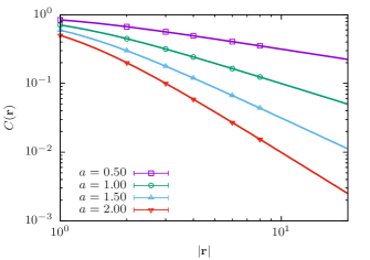
Figure 2: Correlation function $C({\bf r})$ compared to the measured site-site correlation function $\left\langle C_{\bf r}\right\rangle_{R}$ of continuous variables along the $x$-direction on a $16^{2}$ lattice with $R=10^{6}$ disorder replicas. The continuous random variables are obtained via a discrete Fourier transform of $C_{\bf r}$ and satisfy $\sigma^{2}_{\tau}=\left\langle C_{0}\right\rangle_{R}=1$.

III Mapping to long-range correlated defects

To study percolation, we have to map the correlated continuous variables $\tau_{{\bf x}}$ to correlated discrete values $t_{{\bf x}}\in\{0,1\}$. For this, we need to specify the mean density of available sites $p$ (considering defects as $t_{{\bf x}}=0$). Here, we use a global or grand-canonical Wiseman and Domany (1998) approach and fix the expectation value $\left\langle\sum_{\bf x}t_{{\bf x}}/N\right\rangle=\left\langle t\right\rangle=p$. Therefore, we introduce a threshold $\theta$ such that sites are considered defects if $\tau_{{\bf x}}<\theta$. In the disorder average the $\tau_{{\bf x}}$ are normally distributed, such that the threshold is tied to $p$ via

$${p=p(\theta)=\int_{\theta}^{\infty}P(\tau)d\tau=\frac{1}{2}{\rm erfc}\left(\frac{\theta}{\sqrt{2\sigma^{2}_{\tau}}}\right)},$$ (14)

where erfc denotes the standard complementary error function and $\sigma^{2}_{\tau}=1$ by construction. Note that for strong correlations, the densities on individual replica fluctuate significantly. If we measure the site-site correlation function of discrete variables according to Eq. (13) (where we replace $\left\langle\tau\right\rangle$ with $\left\langle t\right\rangle=p$), we observe $\left\langle C_{0}\right\rangle_{R}=\sigma^{2}_{t}<1$. The variance of discrete site variables is no longer unity but is instead connected to the variance of uncorrelated random lattices, $\sigma^{2}_{t}=p(1-p)$. Figure 3 (open symbols) shows the discrete site-site correlation function averaged over $10^{4}$ lattices of size $1024^{2}$. It can be seen that the average site-site correlations on discrete lattices mapped via Eq. (14) decay according to Eq. (12) over a long range, though the amplitudes are somewhat diminished.

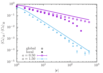
Figure 3: Normalized correlation function of discrete random variables with long-range power-law correlation at the percolation threshold $p_{c}(a)$ (see Table 2) on a $1024^{2}$ lattice averaged over $10^{4}$ disorder replicas. Continuous correlated random variables were obtained as described in Sec. II. The mapping to discrete variables is performed via a global approach (open symbols), i.e., on the level of the disorder average [see Eq. (14)], and via a local approach, i.e., on the level of each disorder realization (filled symbols). The measured site-site correlation function $\left\langle C_{\bf r}\right\rangle_{R}$ along the $x$-axis is normalized with respect to the variance $\left\langle C_{0}\right\rangle_{R}$ for discrete site variables.

Alternatively, one might use a local or canonical Wiseman and Domany (1998) approach, adjusting $\sum_{\bf x}t_{{\bf x}}/N=p$ for each replica by sorting the continuous correlated variables and adjusting $\theta$ until $\sum_{\bf x}\Theta(\tau_{{\bf x}}-\theta)/N=p$, where $\Theta$ is the unit step function Schrenk et al. (2013). However, fixing $p$ on every lattice tends to suppress correlations on a macroscopic scale. As can be seen in Fig. 3 (filled symbols), this results in a decay rate of the correlation function that is faster than polynomial. This effect is most significant for strong correlations and small systems and can be expected to vanish in the limit of infinite system size. By contrast, the global approach Eq. (14) described above works reliably for any lattice size and appears thus generally preferable.

IV Percolation threshold

The value of the percolation threshold $p_{c}$ is not a universal quantity. It may not only depend on the type of lattice but also on local aspects of the correlation function $C_{\bf r}$ and hence on the implementation of the FFM. Numerical results given in this section therefore only apply for the specific settings we used and cannot be quantitatively compared to those from previous studies, e.g., Ref. Prakash et al. (1992). We were careful to be explicit about these settings to ensure that our results for the fractal dimensions are reproducible, and so that future studies may use our estimates for $p_{c}$.

We use the correlation function Eq. (12) and perform a discrete numerical Fourier transform as discussed in the previous section. The radial distance $|{\bf r}|$ is usually considered in the Euclidean metric, but here we also use the Manhattan metric, i.e., the minimum number of steps on the lattice. This is done to demonstrate the sensitivity of $p_{c}$ to changes of the correlation function that are not captured in the correlation parameter $a$. Later, we also use the Manhattan metric to test the robustness of our estimates for the fractal dimensions, which should be the same for both variants.

To define percolation on a finite lattice, we apply the horizontal wrapping criterion: a cluster percolates if it closes back on itself across one specific lattice boundary. This choice has the benefit of being translationally invariant and is known to give relatively small finite-size errors Newman and Ziff (2001). The percolation threshold $p_{c}^{L}$ for the finite system of extension $L$ is then defined as the average occupation density at which a percolating cluster emerges. We estimate this value by determining the maximum threshold $\theta_{c}$ for each replica of continuous variables at which a percolating cluster exists for the subset of sites with $\tau_{{\bf x}}\geq\theta_{c}$. We then take the average of the mapped values,

$$p_{c}^{L}=\left\langle p\left(\theta_{c}\right)\right\rangle,$$ (15)

where the mapping is carried out according to Eq. (14).

IV.1 Square lattice

Table 1: Estimates of the percolation threshold for square lattices with correlated disorder. For consistency all fits include $L\geq 64$.The extended Harris criterion, Eq. (2), modifies $\nu_{a}\neq\nu$ for $a<2/\nu=1.5$.

$a$	$\nu_{a}$	$p_{c}$ (Euclid.)	$\chi^{2}/{\rm{dof}}$	$p_{c}$ (Manh.)	$\chi^{2}/{\rm{dof}}$
$\infty$	$4/3$ Nienhuis (1984)	$0.592746$ Ziff (1992)
3	$4/3$	$0.561406(4)$	0.92
2.5	$4/3$	$0.556214(4)$	0.87
2	$4/3$	$0.550143(5)$	0.90	$0.528397(5)$	1.9
1.75	$4/3$	$0.546717(7)$	0.41
1.5	$4/3$	$0.54299(1)$	3.5	$0.519991(8)$	4.0
1.25	$8/5$	$0.53895(2)$	1.4
1	$2$	$0.53452(4)$	0.87	$0.51226(4)$	2.28
0.75	$8/3$	$0.5296(1)$	0.63
0.5	$4$	$0.5239(3)$	0.53	$0.5054(3)$	0.66
0.25	$8$	$0.516(1)$	0.38
0.1	$20$	$0.508(4)$	1.2

In $2D$, we extrapolate to the percolation threshold for the infinite system, $p_{c}:=p_{c}^{\infty}$, via the standard finite-size scaling approach Stauffer and Aharony (1992) without higher-order correction terms

$${|p_{c}-p^{L}_{c}|}\sim L^{-1/\nu_{a}}.$$ (16)

Here $\nu_{a}$ denotes the critical exponent of the correlation length. The value of $\nu_{a}$ is determined by Eq. (2) with the uncorrelated correlation-length exponent $\nu=4/3$ Stauffer and Aharony (1992). This assumed behavior of $\nu_{a}$ has been numerically supported for percolation on a $2D$ triangular lattice Schrenk et al. (2013).

To obtain our numerical estimates, we randomly generated $10^{5}$ replicas for each size $L=2^{l}$ where $l=6,\ldots,13$ ($L=64$–$8192$). Some of the results for $p^{L}_{c}$ are shown in Fig. 4 (top) together with least-squares fits of Eq. (16) over the range $L\geq 64$. The estimates for $p_{c}$ are the $y$-intercepts of the fit curves. The values are listed in Table 1, where we also give the reduced $\chi^{2}$-values per degree-of-freedom (dof) of the respective fits. The last columns show our results for systems where the Manhattan metric is used to set the distance $|{\bf r}|$ for the correlations. Here the estimates for $p_{c}$ are considerably smaller than for the Euclidean case, underlining the strong dependence of $p_{c}$ on the details of the correlation function. In both cases the $\chi^{2}$-values are mostly close to one, justifying the simple scaling ansatz. However, they are quite large at the “crossover” value of $a_{\rm H}=1.5$, where the behavior is supposed to change according to the extended Harris criterion, Eq. (2). This suggests the presence of additional correction terms in the vicinity of $a_{\rm H}$, possibly of logarithmic nature.

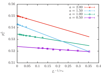
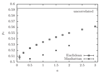
Figure 4: Top: Measured percolation thresholds $p_{c}^{L}$ for varying lattice size $L$ and different values of the correlation parameter $a$ in $2D$ (Euclidean metric). Lines show the best fits of Eq. (16) to the data, whose intercepts represent our estimates for the infinite-system value $p_{c}$. Bottom: Estimates for $p_{c}$ as function of the correlation strength for the square lattice with distances measured in the Euclidean metric (squares) and the Manhattan metric (crosses). The horizontal line shows the value for the system without correlations.

An overview of the results for the percolation thresholds as a function of $a$ is shown in the bottom plot of Fig. 4. As can be seen, correlations tend to lower $p_{c}$, which is intuitive as they promote the emergence of larger clusters. As noted in Ref. Prakash et al. (1992) the value of $p_{c}$ for the square lattice must eventually approach $1/2$. This bound can be understood considering that a cluster of occupied sites that wraps the system in one direction exists if and only if no cluster of defects wraps the system in the orthogonal direction, where the defects are allowed to connect via next-nearest neighbors (diagonally). For $a\longrightarrow 0$, the relevance of these next-nearest neighbor connections becomes negligible, and the resulting symmetry between clusters of defects and occupied sites demands $p_{c}=1/2$. Note that for the Manhattan metric, diagonal correlations are weaker to begin with. The strong deviations do not only depend on the chosen metric but are already affected by the details of the employed method, as can be seen by comparing to results we obtained with the continuous FFM on a square lattice Fricke et al. (2017), which qualitatively look similar but do not agree within error bars.

When $a$ is increased, i.e., when the correlation strength is diminished, $p_{c}$ must converge towards the value for the uncorrelated system as long as $C({\bf r})/C(0)\longrightarrow 0$ for all $|{\bf r}|>0$. Note, however, that the uncorrelated value is only reached in the limit $a\rightarrow\infty$ and not at $a=D$, where the correlations become effectively short range. This is contrary to the results from previous studies due to differing definitions of the correlation function $C({\bf r})$, which at $a=2$ has a vanishing amplitude in Ref. Prakash et al. (1992) and a divergent variance $C(0)$ in Ref. Pang et al. (1995).

IV.2 Cubic lattice

The version of the FFM described in Sect. II can directly be applied in three (or more) dimensions as well, which allowed us to study percolation with long-range correlated disorder on the cubic lattice. We looked at systems with linear extensions in the range $L=8$–$512$, and we again generated $10^{5}$ random replicas for each size. Unlike in $2D$, however, the simple finite-size scaling approach to estimate the percolation threshold $p_{c}$, Eq. (16), proved unsuccessful, suggesting the need of higher-order terms (see Ref. Herrmann and Stauffer (1983) for a discussion of finite-size scaling for uncorrelated systems):

$${|p_{c}-p^{L}_{c}|}\sim L^{-1/\nu_{a}}(A+BL^{-\omega}+CL^{-1/\nu_{a}}+\ldots),$$ (17)

where $\nu_{a}$ is given by Eq. (2) with $\nu$ the correlation-length exponent for uncorrelated percolation (0.8764(12) Wang et al. (2013), 0.8762(12) Xu et al. (2014), 0.8751(11) Hu et al. (2014)).

Table 2: Estimates of the percolation threshold for cubic lattices with correlated disorder. For consistency all fits include $L\geq 32$. The extended Harris criterion, Eq. (2), modifies the correlation-length exponent $\nu_{a}\neq\nu$ for $a<2/\nu\approx 2.28$.

$a$	$\nu_{a}$	$p_{c}$ (Euclid.)	$\chi^{2}/{\rm{dof}}$	$p_{c}$ (Manh.)	$\chi^{2}/{\rm{dof}}$
$\infty$	$0.8762$	0.311610(2)	0.44
4	$0.8762$	0.238778(4)	0.10
3	$0.8762$	0.208438(5)	0.83	0.209315(4)	0.75
2.5	$0.8762$	0.188289(7)	1.9	0.189801(5)	6.0
2	$1$	0.16302(2)	3.0	0.16514(1)	0.54
1.5	$4/3$	0.13022(5)	0.51	0.13251(4)	0.37
1	$2$	0.0863(3)	1.1	0.0878(2)	0.86
0.5	$4$	0.025(3)	1.4	0.030(2)	0.25

In practice, the correction to Eq. (16) seems to be described well by the latter (quadratic) term alone, suggesting that the correction-to-scaling exponent $\omega$ is relatively large. This is in fact the case for the uncorrelated system, where previous estimates locate the correction-to-scaling exponent between $\omega\approx 1.62$ Ballesteros and Parisi (1999) and $\omega\approx 1.2$ Wang et al. (2013). We thus used the ansatz

$${|p_{c}-p^{L}_{c}|}\sim L^{-1/\nu_{a}}(A+CL^{-1/\nu_{a}}),$$ (18)

which we fitted to the data for $L\geq 32$. The corresponding fit curves and our results for $p_{c}^{L}(a)$ are shown for selected correlations in Fig. 5 (top), and the resulting estimates for $p_{c}=p_{c}^{\infty}$ are listed in Table 2. Again, we see that the changing behavior predicted by the extended Harris criterion (at $a_{\rm H}=2/\nu\approx 2.28$) manifests itself in a poorer quality of the fits for nearby values ($a=2$ and $a=2.5$). Our estimate for the uncorrelated case, $p_{c}(\infty)=0.311\,610(2)$, is in decent agreement with previous estimates ($0.311\,608\,1(11)$ Ballesteros and Parisi (1999), $0.311\,607\,7(2)$ Wang et al. (2013), 0.311 607 68(15) Xu et al. (2014)).

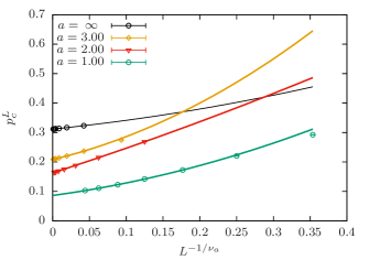
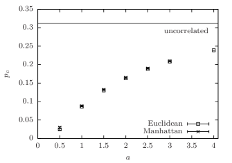
Figure 5: Top: Measured percolation thresholds $p_{c}^{L}$ for varying lattice size $L$ and different values of the correlation parameter $a$ in $3D$ (Euclidean metric). Lines show the best fits of Eq. (18) to the data, whose intercepts represent our estimates for the infinite-system value $p_{c}$. Bottom: Estimates for $p_{c}$ as function of the correlation strength for the cubic lattice with distances measured in the Euclidean metric (squares) and the Manhattan metric (crosses). The horizontal line shows the value for the system without correlations.

In contrast to the $2D$ situation, using the Manhattan metric in place of the Euclidean metric to measure the distance for the correlation function does not significantly lower the percolation threshold. As can be seen in Table 2 and Fig. 5 (bottom), the values are even slightly larger. That is plausible since the argument why the Manhattan metric should lower $p_{c}$ in $2D$ does not apply in $3D$, where wrapping clusters of defects and occupied sites can coexist. This also means that there is no obvious lower bound for $p_{c}$ in $3D$ other than zero. Indeed, our estimates for strong correlations are very small, and the overview shown in Fig. 5 (bottom) even seems to suggest the extrapolation $p_{c}\rightarrow 0$ for $a\rightarrow 0$.

We should note, however, that the scaling ansatz Eq. (18) is mainly motivated empirically. Especially for small $a$, some of the finite-size corrections have a different origin as in the uncorrelated system, namely that smaller systems are not self-averaging: For small $a$ and small $L$, the continuous site variables $\tau_{{\bf x}}$ within each individual replica tend to be very similar, and about half the ensemble has mostly negative values, while the other has mostly positive values. In the limit $a\rightarrow 0$ (at fixed $L$) the values $\tau_{{\bf x}}$ across each replica become constant, so that a wrapping cluster in the discrete system emerges when a threshold $\theta_{c}=\tau_{{\bf x}}$ is used for the mapping. Since the overall distribution of the $\tau$-values is symmetric (Gaussian) and we define $p^{L}_{c}$ according to Eq. (14) and Eq. (15), the $a\rightarrow 0$ limit at fixed $L$ is $p^{L}_{c}(0)=1/2$. This “segregation” finite-size effect might play a significant role for the most strongly correlated cases ($a=\{0.5,1\}$), and our respective estimates should therefore be taken with a pinch of salt.

Table 3: Fractal dimension for square lattices with correlated disorder. For consistency all fits include sizes $L\geq 128$. In two dimensions we consider only the leading-order behavior at the finite-size percolation transition. Results from Euclidean and Manhattan metric are in good agreement.

$a$	$d_{\mathrm{f}}$ (Euclid.)	$\chi^{2}/{\rm{dof}}$	$d_{\mathrm{f}}$ (Manh.)	$\chi^{2}/{\rm{dof}}$
$\infty$	$91/48\approx 1.89583...$
3	1.8961(2)	0.74
2.5	1.8962(2)	1.2
2	1.8966(2)	4.5	1.8964(2)	1.2
1.75	1.8964(2)	2.8
1.5	1.8965(3)	1.6	1.8956(3)	2.3
1.25	1.8950(3)	1.2
1	1.8961(3)	1.2	1.8952(3)	0.29
0.75	1.9006(4)	1.2
0.5	1.9128(5)	0.47	1.9126(6)	0.17
0.25	1.9360(6)	0.085
0.1	1.9602(8)	0.39

V Fractal Dimension

The fractal dimension $d_{\mathrm{f}}$ describes how the volume of a critical percolation cluster increases with its linear size. It can conveniently be estimated via

$$\left\langle V\right\rangle\sim L^{d_{\mathrm{f}}},$$ (19)

where $L$ is the lattice extension and $\left\langle V\right\rangle$ denotes the average number of sites in the largest cluster Stauffer and Aharony (1992). Note that for correlated systems, it is important to include replicas with no percolating cluster. It is possible to either consider all systems at the same, asymptotic concentration $p_{c}$ or to take size-dependent values, $p^{L}_{c}$. We opted for the latter approach, so we would not have to rely on the fitting ansatz for $p_{c}$.

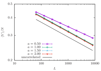
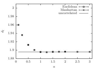
Figure 6: Top: Average volume fraction of the largest cluster vs. lattice extension in $2D$ plotted for different correlations $a$ on a double-logarithmic scale (Euclidean metric). Colored lines are least-squares fits to Eq. (19). The black line represents the behavior of the uncorrelated system with a slope of $91/48-2$. Bottom: Overview of our estimates for the fractal dimensions as function of $a$ with the horizontal line again corresponding to the uncorrelated system.

V.1 Square lattice

In $2D$, finite-size corrections again turned out to be small, so that fitting Eq. (19) without any higher-order correction terms worked well. Figure 6 (top) shows the average volume of the largest cluster relative to the total number of sites, $\left\langle V\right\rangle/L^{D}$, for several different values of $a$ plotted on a double-logarithmic scale. The lines correspond to least-squares fits of Eq. (19) over the range $L\geq 128$, and their slopes show the differences to the Euclidean dimension, $d_{\mathrm{f}}-2$. Our resulting estimates for $d_{\mathrm{f}}$ can be found in Table 3 together with the reduced $\chi^{2}$-values of the fits. Also listed are estimates obtained using the Manhattan instead of the Euclidean metric. Here, the fits yielded smaller amplitudes, but the exponents resulted very similar. This can be seen in Fig. 6 (bottom), which shows an overview of the estimates for $d_{\mathrm{f}}$. The data verifies that $d_{\rm f}$ is universal, i.e., independent of system details. For weak correlations the uncorrelated value, $d_{\rm f}=91/48$ Nienhuis (1984), seems to be recovered in accordance with the extended Harris criterion [Eq. (2)] and earlier numerical findings Prakash et al. (1992); Makse et al. (1995b, 1998); Schrenk et al. (2013). Interestingly though, there seems to be no increase of $d_{\mathrm{f}}$ directly below $a_{\rm H}=3/2$, the crossover threshold set by the extended Harris criterion. For the Manhattan metric, the fit quality is still diminished around $a_{\rm H}$, suggesting that the threshold may still affect correction terms. However, it is yet unclear why $\chi^{2}$ is largest at $a=2$ for the Euclidean case.

The fact that $d_{\mathrm{f}}$ does not increase directly below $a_{\rm H}$ was already noted in Ref. Schrenk et al. (2013), where a crossover threshold of $a_{\rm x}=2/3$ (or in terms of the Hurst exponent $H_{\rm x}=-a_{\rm x}/2=-1/3$) was suggested instead. However, that value is not quite consistent with our findings, which show a significant increase already at $a>3/4$. Another disagreement regards the behavior in the correlated limit, $a\rightarrow 0$ ($H\rightarrow 0$): our results are consistent with the idea that the fractal dimension converges to the “Euclidean” value of $D=2$ as clusters get more and more compact, while according to Ref. Schrenk et al. (2013) the value stays well below $2$. This discrepancy may be owed to the use of different mapping rules as discussed at the end of Sec. III.

It is interesting to compare the results for $d_{\rm f}$ with the Ising model at criticality, which exhibits spin-spin correlations of the form $\langle S_{i}S_{j}\rangle\sim r^{-(d-2+\eta)}$. In two dimensions $\eta=1/4$ and the fractal dimension of the geometrical Ising clusters is $d_{\mathrm{f}}=187/96=1.9479\ldots$ Stella and Vanderzande (1989); Duplantier and Saleur (1989), which is indeed quite similar to our result of $d_{\mathrm{f}}=1.9360(6)$ for $a=1/4$. As already noted Prakash et al. (1992), the results could not be expected to agree perfectly. In fact, it is intuitive that $d_{\mathrm{f}}$ should be slightly larger for Ising clusters, where the spin-spin correlation function is essentially the probability that two spins belong to the same cluster. In our system, by contrast, spins from unconnected clusters still contribute to the correlation function, so that connected clusters may be “thinner” for the same decay exponent.

Table 4: Fractal dimension for cubic lattices with correlated disorder. For consistency all fits include sizes $L\geq 16$. In three dimensions, we require higher-order corrections of the form Eq. (20). Assuming universality, we perform simultaneous fits including both Euclidean and Manhattan metric.

$a$	$d_{\mathrm{f}}$	$w$	$\chi^{2}/{\rm{dof}}$
$\infty$	2.52295(15) Wang et al. (2013)	1.2(2) Wang et al. (2013)
3	2.524(2)	1.2(2)	0.70
2.5	2.522(2)	0.9(2)	3.3
2	2.512(3)	0.9(2)	1.9
1.5	2.507(6)	0.6(1)	0.55
1	2.6(2)	0.20(1)	2.1

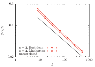
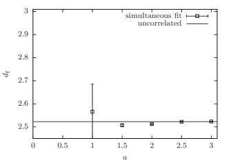
Figure 7: Top: Average volume fraction of the largest cluster vs. lattice extension in $3D$ plotted for the exemplary case $a=2$ on a double-logarithmic scale. Colored lines are the simultaneous fits according to Eq. (20); the black line represents the behavior of the uncorrelated system with a slope of $2.52295-3$. Bottom: Overview of our estimates for the fractal dimensions as function of $a$ with the horizontal line again corresponding to the uncorrelated system. Our fitting did not work properly for very strong correlations ($a\leq 1$).

V.2 Cubic lattice

The situation in $3D$ turned out to be more difficult. As with the percolation threshold, the scaling behavior seems to involve strong finite-size corrections, so that simply fitting Eq. (19) would not work for the system sizes that we considered. Including a correction term also failed as the fit could not handle two additional parameters. What did work reasonably well, at least for $a>1$, was fitting our data for the Euclidean and the Manhattan versions simultaneously, while assuming the exponents of the leading term and the correction to be equal for both cases:

$$\left\langle V\right\rangle_{\mathrm{Euclid.}} =A_{1}L^{d_{\mathrm{f}}}(1+B_{1}L^{-w}),$$

$$\left\langle V\right\rangle_{\mathrm{Manh.}} =A_{2}L^{d_{\mathrm{f}}}(1+B_{2}L^{-w}).$$ (20)

This approach was motivated by general universality arguments Cardy (1996); Zinn-Justin (2007) and our previous observation that the fractal dimensions in $2D$ are the same for both versions. We assume that equality also holds for the correction exponents $\omega$, which seems reasonable since $\omega$ is also strongly believed to be universal for percolation without correlations, see for instance Ref. Ballesteros et al. (1999). Figure 7 shows finite-size scaling data and fits for the case $a=2$ as an example (top) and an overview of the obtained estimates for $d_{\mathrm{f}}$ (bottom). The values of our estimates can be found in Table 4 together with the correction exponents and the $\chi^{2}$-values of the fits. Unfortunately, the data for $a\leq 1$ could not be convincingly fitted by this approach. For these strongly correlated cases, one would probably need to investigate systems still much larger than $512^{3}$. For $a\geq 1.5$, the value for $d_{\mathrm{f}}$ seems to be very similar to the one without correlations ($d_{\rm f}(\infty)=2.522\,95(15)$ Wang et al. (2013)). As in $2D$, the Harris threshold, $a_{\rm H}=2/\nu\approx 2.28$, does hence not determine the onset of a sudden increase in the fractal dimension. Surprisingly, the value even seems to decrease slightly below $a_{\rm H}$. At close inspection, this can also be observed in $2D$ for $a=1.25<a_{\rm H}$, compare Table 3. A diminishing fractal dimension does not seem plausible as stronger correlations should make the clusters more compact. We suspect that a correction term comes into play at $a_{\rm H}$ which is not captured by our fitting approach.

VI Conclusions

We presented high-precision results for the percolation thresholds on square and cubic lattices with long-range power-law correlated disorder as well as estimates for the fractal dimensions of the critical percolation clusters. The correlations were generated using the Fourier filtering method (FFM) based on the discrete Fourier transform. We specified the details of our implementation, so that it may easily be reproduced Note (1) and discussed the differences to previous approaches regarding, e.g., how the continuous site variables are mapped to discrete disorder.

The percolation threshold is dependent on the employed method and moreover on short-range details of the model. We demonstrated this by using both the standard Euclidean metric and the discrete Manhattan metric to define the correlation. The effect of this choice on the percolation threshold is particularly strong for the square lattice. This is because diagonal correlations are weaker for the Manhattan metric, bringing the system closer to $p_{c}=0.5$ where the percolation thresholds for occupied sites and defects connected via next-nearest (diagonal) neighbors coincide. In general, correlations were shown to lower $p_{c}$, and in three dimensions the value even becomes very close to zero for small $a$, i.e., strong correlations.

The fractal dimension, by contrast, is a universal quantity and does not depend on details of the model. We verified that for large $a$ (weak correlations) the fractal dimension of the uncorrelated model is reproduced showing $d_{\rm f}\approx 91/48$ ($2D$) and $d_{\rm f}\approx 2.52$ ($3D$). This was expected above the bound from the extended Harris criterion, i.e., for all $a\geq a_{\rm H}$ with $a_{\rm H}=1.5$ ($2D$) and $a_{\rm H}\approx 2.28$ ($3D$). However, as was previously noticed for the triangular lattice Schrenk et al. (2013), $d_{\rm f}\approx d_{\rm f}^{\rm uncorr}$ seems to remain true also well below the Harris bound. In two dimensions, our data suggests that the value of $d_{\rm f}$ starts to rise below $a_{\rm x}\approx 1$, approaching $d_{\rm f}\rightarrow 2$ as $a\rightarrow 0$. Differences to previous findings may be attributed to different mapping prescriptions employed. To obtain estimates for $d_{\rm f}$ in three dimensions, we simultaneously fitted our data for correlations with Euclidean and Manhattan metric using a polynomial fit with a correction term. Unfortunately, this approach did not work for very strong correlations, i.e., for $a\leq 1$. In the accessible range, the values were found very close to the uncorrelated value. Below $a_{\rm H}\approx 2.28$, they even resulted slightly smaller, which we suspect is due to changing corrections to scaling. We conclude that while the bound from the Harris criterion does not seem to determine a change in the leading exponent $d_{\rm f}$, it does affect the system’s sub-leading behavior.

Appendix A Discrete Wiener-Khinchin theorem

We require $\varphi_{{\bf x}}$ to be complex random variables with independent real and imaginary contributions. For a given disorder realization the lattice average of $\varphi_{{\bf x}}^{*}\varphi_{{\bf x}+{\bf r}}^{\phantom{\ast}}$ can be written as

$$\frac{1}{N} \sum_{\bf x}\varphi_{{\bf x}}^{*}\varphi_{{\bf x}+{\bf r}}^{\phantom{*}}$$

$$=\frac{1}{N}\sum_{\bf x}\left(\frac{1}{N}\sum_{\bf k}\varPhi_{{\bf k}}^{*}e^{\frac{2\pi i{\bf k}{\bf x}}{L}}\right)\left(\frac{1}{N}\sum_{\bf l}\varPhi_{{\bf l}}e^{-\frac{2\pi i{\bf l}({\bf x}+{\bf r})}{L}}\right)$$

$$=\frac{1}{N^{2}}\sum_{\bf k}\varPhi_{{\bf k}}^{*}\sum_{\bf l}\varPhi_{{\bf l}}e^{-\frac{2\pi i{\bf l}{\bf r}}{L}}\frac{1}{N}\sum_{\bf x}e^{\frac{2\pi i({\bf k}-{\bf l}){\bf x}}{L}}$$

$$=\frac{1}{N^{2}}\sum_{\bf k}\varPhi_{{\bf k}}^{*}\sum_{\bf l}\varPhi_{{\bf l}}e^{-\frac{2\pi i{\bf l}{\bf r}}{L}}\delta_{{\bf l},{\bf k}}$$

$$=\frac{1}{N^{2}}\sum_{\bf k}|\varPhi_{{\bf k}}|^{2}e^{-\frac{2\pi i{\bf k}{\bf r}}{L}}.$$ (21)

Here, we used the notation of a $D$-dimensional Kronecker-Delta function $\delta_{{\bf l},{\bf k}}=\Pi_{i}\delta_{l_{i},k_{i}}=\frac{1}{L^{D}}\sum_{\bf x}e^{2\pi i({\bf k}-{\bf l}){\bf x}/L}$. The result is essentially the discrete Wiener-Khinchin theorem, a special case of the cross-correlation theorem.

Taking the disorder average on both sides of Eq. (21) and exploiting translational invariance on the left, we thus obtain

$$\left\langle\varphi_{{\bf x}}^{*}\varphi_{{\bf x}+{\bf r}}^{\phantom{*}}\right\rangle =\frac{1}{N^{2}}\sum_{\bf k}\left\langle|\varPhi_{{\bf k}}|^{2}\right\rangle e^{-\frac{2\pi i{\bf k}{\bf r}}{L}}.$$ (22)

Appendix B Effect of zero-cutoff in $S_{\bf k}$ on $C_{\bf r}$

As mentioned in Sec. II, particular choices of $C({\bf r})$ evaluated on a finite lattice may lead to unphysical negative values of the discrete spectral density $S_{\bf k}$. This seems to occur only for strong correlations (small $a$) and becomes more noticeable with increasing dimension. Numerically, we deal with this issue by a zero-cutoff, i.e., by using a modified spectral density

$$\widetilde{S}_{\bf k}=\begin{cases}S_{\bf k},\quad&\mathrm{if}\>S_{\bf k}\geq 0\\ 0,&\mathrm{else.}\end{cases}$$ (23)

This inevitably affects the resulting correlation function. We can directly predict the effect from the inverse discrete Fourier transform of $\widetilde{S}_{\bf k}$ since

$$\widetilde{C}_{\bf r}=\frac{1}{N}\sum_{{\bf k}}\widetilde{S}_{{\bf k}}e^{-\frac{2\pi i{\bf k}{\bf r}}{L}}$$ (24)

is of course the asymptotic limit of the measured site-site correlation function $\left\langle C_{\bf r}\right\rangle_{R}$ for large sample size $R$.

It turns out that the effect of this zero-cutoff is very small, if present at all, with deviations mainly occurring for small lattices. With increasing lattice size, the predicted (and measured) deviations quickly converge towards the desired correlation function. To demonstrate this, we consider the example of three-dimensional lattices with (strong) correlations $a=0.5$ and linear extensions $L=\{8,16,32\}$ in Fig. 8. The measured correlation function of continuous site variables along the $x$-direction $\left\langle C_{\bf r}\right\rangle_{R}$ [Eq. (13)], is evaluated with data from Sec. IV. The effect of the zero-cutoff on the correlation function from Eq. (12) is indeed perfectly predicted by Eq. (24).

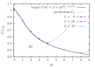
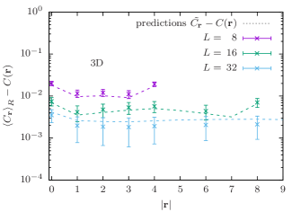
Figure 8: (Top) Demonstration of the effect of the zero-cutoff $S_{\bf k}\rightarrow\widetilde{S}_{\bf k}$ on the measured correlation function $\left\langle C_{\bf r}\right\rangle_{R}$ in three dimensions for $a=0.5$. Also shown is the prediction $\widetilde{C}_{\bf r}$ for the asymptotic limit from Eq. (24). (Bottom) Plot of the deviations from the desired function $C({\bf r})$.

Appendix C Different versions of the FFM

Many different variants of the FFM can be found in the literature Peng et al. (1991); Prakash et al. (1992); Pang et al. (1995); Makse et al. (1995a, 1996); Ballesteros and Parisi (1999); Ahrens and Hartmann (2011); Simon et al. (2012). We want to give a brief overview of the differences and discuss the effects of some of the implied approximations.

In early works the spectral density is approximated as $S({\bf q})=|{\bf q}|^{-(D-a)}$ Prakash et al. (1992). The resulting non-trivial amplitude in the correlation function $C({\bf r})=f(D-a)|{\bf r}|^{-a}$ was shown to vanish for $a\rightarrow D$, in accordance with the picture that the uncorrelated case should be recovered for short-range correlations ($a>D$). Still, the desired correlation function could only be produced in a small region of the system with this approach.

Reference Pang et al. (1995) follows a similar idea, but directly uses $C({\bf r})=|{\bf r}|^{-a}$. This function diverges at $|{\bf r}|=0$, and hence the authors interpolate by integrating the function in the corresponding discrete bin around zero. This works reliably in one dimension but becomes cumbersome in more dimensions. Moreover, this assigns a non-trivial value to $C(0)$ thus modifying the variance of the desired Gaussian random variables.

The most influential works are by Makse et al. Makse et al. (1995a, 1996). They introduced the correlation function from Eq. (12), allowing them to approach the problem both numerically Makse et al. (1995a) and (partially) analytically Makse et al. (1996). Their numerical approach is quite similar to ours, but the analytical one has received far more attention. We have in fact tried it ourselves Fricke et al. (2017), but found that it has many pitfalls, which we want to briefly discuss here. The idea is to discretize the Fourier transform of $C({\bf r})=(1+{\bf r}^{2})^{-a/2}$ for the infinite continuum, which can be calculated analytically:

$$S({\bf q}) =\int_{-\infty}^{\infty}C({\bf r})e^{i{\bf q}{\bf r}}d{\bf r}$$

$$=\frac{2\pi^{D/2}}{\Gamma(a/2)}\left(\frac{|{\bf q}|}{2}\right)^{\beta}K_{\beta}(|{\bf q}|),$$ (25)

where $\Gamma$ is Euler’s gamma function and $K_{\beta}(|{\bf q}|)$ is the modified Bessel function of order $\beta=(a-D)/2$ . The variance is recovered by integrating over full continuous space $\sigma^{2}_{\tau}=C(0)=\frac{1}{2\pi}\int_{-\infty}^{\infty}S({\bf q})d{\bf q}=1$.

The next step is to identify $q=\frac{2\pi}{L}{\bf k}$ and map the continuous result to a discrete lattice by evaluating the function $S(\frac{2\pi}{L}{\bf k})$ at each lattice site ${\bf k}$. The first problem here is that $S({\bf 0})$ diverges. This can be circumvented by evaluating the zero-signal at a shifted frequency, i.e., $S_{\bf 0}=S(\frac{2\pi}{L}|{\bf k}|_{0})$ with $|{\bf k}|_{0}\in(0,1)$ chosen “appropriately” Makse et al. (1996). With increasing system size the choice becomes less relevant, and the differences can be expected to vanish in the infinite-system limit. For finite systems, however, the effect of the parameter $|{\bf k}|_{0}$ depends on the dimension and the strength of the correlations. In addition, $|{\bf k}|_{0}$ has to be adjusted iteratively, rendering the application of the method rather tedious.

There is another, more severe problem with the discretization, which is relevant for the mapping to discrete site variables Fricke et al. (2017) (see Sec. III). As we are interested in the asymptotic long-range scaling behavior, we typically use a fixed lattice spacing of unit length $\Delta x_{i}=1$ and consider the limit to infinite system size rather than to the continuum. Thus, the frequency space is confined to $q_{i}\in[-\pi,\pi)$, while the resolution increases with increasing system size. As a consequence, the variance $\sigma^{2}_{\tau}$ will deviate from one, complicating the mapping procedure. In fact, we can estimate the deviations via $\sigma^{2}_{\tau}=\frac{1}{2\pi}\int_{-\pi}^{\pi}S({\bf q})d{\bf q}\leq 1=C(0)$. We numerically verified this but also found additional finite-size scaling corrections of the form $\sigma^{2}_{\tau,L}=\sigma^{2}_{\tau}+\mathcal{O}(L^{-1})$. These corrections are inconvenient for finite-size scaling, e.g., for finding the percolation threshold, because one needs to evaluate the variance $\sigma^{2}_{\tau,L}$ in addition to the parameter $|{\bf k}|_{0}$ for each value of the correlation parameter $a$ and each system size. By contrast, the method sketched in Sec. II is parameter free and always yields the correct variance $\sigma^{2}_{\tau}$ up to negligible effects from the zero-cutoff.

References

- Pfeifer and Avnir (1983) P. Pfeifer and D. Avnir, “Chemistry in noninteger dimensions between two and three. I. Fractal theory of heterogeneous surfaces,” J. Chem. Phys. 79, 3558 (1983).
- Avnir et al. (1984) D. Avnir, D. Farin, and P. Pfeifer, “Molecular fractal surfaces,” Nature 308, 261 (1984).
- Dorogovtsev (1980) S. N. Dorogovtsev, “Critical exponents of magnets with lengthy defects,” Phys. Lett. A 76, 169 (1980).
- Yamazaki et al. (1986) Y. Yamazaki, A. Holz, M. Ochiai, and Y. Fukuda, “Static and dynamic critical behavior of extended-defect -component systems in cubic anisotropic crystals,” Phys. Rev. B 33, 3460 (1986).
- Bouchaud and Georges (1990) J.-P. Bouchaud and A. Georges, “Anomalous diffusion in disordered media: Statistical mechanisms, models and physical applications,” Phys. Rep. 195, 127 (1990).
- Malek and Coppens (2001) K. Malek and M.-O. Coppens, “Effects of surface roughness on self- and transport diffusion in porous media in the Knudsen regime,” Phys. Rev. Lett. 87, 125505 (2001).
- Foulaadvand and Sadrara (2015) M. E. Foulaadvand and M. Sadrara, “Dynamics of a rigid rod in a disordered medium with long-range spatial correlation,” Phys. Rev. E 91, 012122 (2015).
- Goychuk et al. (2017) I. Goychuk, V. O. Kharchenko, and R. Metzler, “Persistent Sinai type diffusion in Gaussian random potentials with decaying spatial correlations,” Phys. Rev. E 96, 052134 (2017).
- Dullien (1979) F. A. L. Dullien, Porous Media: Fluid Transport and Pore Structure (Academic Press, New York, 1979).
- Sahimi (1995) M. Sahimi, Flow and Transport in Porous Media and Fractured Rock (VCH, Weinheim, 1995).
- Skinner et al. (2013) T. O. E. Skinner, S. K. Schnyder, D. G. A. L. Aarts, J. Horbach, and R. P. A. Dullens, “Localization dynamics of fluids in random confinement,” Phys. Rev. Lett. 111, 128301 (2013).
- Spanner et al. (2016) M. Spanner, F. Höfling, S. C. Kapfer, K. R. Mecke, G. E. Schröder-Turk, and T. Franosch, “Splitting of the universality class of anomalous transport in crowded media,” Phys. Rev. Lett. 116, 060601 (2016).
- Bancaud et al. (2012) A. Bancaud, C. Lavelle, S. Huet, and J. Ellenberg, “A fractal model for nuclear organization: Current evidence and biological implications,” Nucleic Acids Res. 40, 8783 (2012).
- Höfling and Franosch (2013) F. Höfling and T. Franosch, “Anomalous transport in the crowded world of biological cells,” Rep. Prog. Phys. 76, 046602 (2013).
- Stauffer and Aharony (1992) D. Stauffer and A. Aharony, Introduction to Percolation Theory (Taylor and Francis, London, 1992).
- Weinrib and Halperin (1983) A. Weinrib and B. I. Halperin, “Critical phenomena in systems with long-range-correlated quenched disorder,” Phys. Rev. B 27, 413 (1983).
- Weinrib (1984) A. Weinrib, “Long-range correlated percolation,” Phys. Rev. B 29, 387 (1984).
- Harris (1974) A. B. Harris, “Effect of random defects on the critical behaviour of Ising models,” J. Phys. C 7, 1671 (1974).
- Prudnikov and Fedorenko (1999) V. V. Prudnikov and A. A. Fedorenko, “Critical behaviour of 3D systems with long-range-correlated quenched disorder,” J. Phys. A: Math. Gen. 32, L399 (1999).
- Prudnikov et al. (2000) V. V. Prudnikov, P. V. Prudnikov, and A. A. Fedorenko, “Field-theory approach to critical behavior of systems with long-range-correlated defects,” Phys. Rev. B 62, 8777 (2000).
- Schrenk et al. (2013) K. J. Schrenk, N. Posé, J. J. Kranz, L. V. M. van Kessenich, N. A. M. Araújo, and H. J. Herrmann, “Percolation with long-range correlated disorder,” Phys. Rev. E 88, 052102 (2013).
- Prakash et al. (1992) S. Prakash, S. Havlin, M. Schwartz, and H. E. Stanley, “Structural and dynamical properties of long-range correlated percolation,” Phys. Rev. A 46, R1724 (1992).
- Makse et al. (1998) H. A. Makse, J. S. Andrade Jr., M. Batty, S. Havlin, and H. E. Stanley, “Modeling urban growth patterns with correlated percolation,” Phys. Rev. E 58, 7054 (1998).
- Saupe (1988) D. Saupe, “Algorithms for random fractals,” in The Science of Fractal Images, edited by H.-O. Peitgen and D. Saupe (Springer, New York, 1988) pp. 71–136.
- Peng et al. (1991) C.-K. Peng, S. Havlin, M. Schwartz, and H. E. Stanley, “Directed-polymer and ballistic-deposition growth with correlated noise,” Phys. Rev. A 44, R2239 (1991).
- Makse et al. (1995a) H. A. Makse, S. Havlin, H. E. Stanley, and M. Schwartz, “Novel method for generating long-range correlations,” Chaos, Solitons & Fractals 6, 295 (1995a).
- Pang et al. (1995) N.-N. Pang, Y.-K. Yu, and T. Halpin-Healy, “Interfacial kinetic roughening with correlated noise,” Phys. Rev. E 52, 3224 (1995).
- Makse et al. (1996) H. A. Makse, S. Havlin, M. Schwartz, and H. E. Stanley, “Method for generating long-range correlations for large systems,” Phys. Rev. E 53, 5445 (1996).
- Ballesteros and Parisi (1999) H. G. Ballesteros and G. Parisi, “Site-diluted three-dimensional Ising model with long-range correlated disorder,” Phys. Rev. B 60, 12912 (1999).
- Ahrens and Hartmann (2011) B. Ahrens and A. K. Hartmann, “Critical behavior of the random-field Ising magnet with long-range correlated disorder,” Phys. Rev. B 84, 144202 (2011).
- Simon et al. (2012) M. S. Simon, J. M. Sancho, and A. M. Lacasta, “On generating random potentials,” Fluct. Noise Lett. 11, 1250026 (2012).
- Note (1) Our code (C++) is available at github.com/CQT-Leipzig/correlated_disorder.
- Press et al. (2007) W. H. Press, S. A. Teukolsky, W. T. Vetterling, and B. P. Flannery, Numerical Recipes 3rd edition: The Art of Scientific Computing (Cambridge University Press, Cambridge, 2007).
- Wiseman and Domany (1998) S. Wiseman and E. Domany, “Self-averaging, distribution of pseudocritical temperatures, and finite size scaling in critical disordered systems,” Phys. Rev. E 58, 2938 (1998).
- Newman and Ziff (2001) M. E. J. Newman and R. M. Ziff, “Fast Monte Carlo algorithm for site or bond percolation,” Phys. Rev. E 64, 016706 (2001).
- Nienhuis (1984) B. Nienhuis, “Critical behavior of two-dimensional spin models and charge asymmetry in the Coulomb gas,” J. Stat. Phys. 34, 731 (1984).
- Ziff (1992) R. M. Ziff, “Spanning probability in 2D percolation,” Phys. Rev. Lett. 69, 2670 (1992).
- Fricke et al. (2017) N. Fricke, J. Zierenberg, M. Marenz, F. P. Spitzner, V. Blavatska, and W. Janke, “Scaling laws for random walks in long-range correlated disordered media,” Condens. Matter Phys. 20, 13004 (2017).
- Herrmann and Stauffer (1983) H. J. Herrmann and D. Stauffer, “Corrections to scaling and finite size effects,” Phys. Lett. A 100, 366 (1983).
- Wang et al. (2013) J. Wang, Z. Zhou, W. Zhang, T. M. Garoni, and Y. Deng, “Bond and site percolation in three dimensions,” Phys. Rev. E 87, 052107 (2013).
- Xu et al. (2014) X Xu, H Wang, J.-P. Lv, and Y. Deng, “Simultaneous analysis of three-dimensional percolation models,” Front. Phys. 9, 113 (2014).
- Hu et al. (2014) H. Hu, H. W. J. Blöte, R. M. Ziff, and Y. Deng, “Short-range correlations in percolation at criticality,” Phys. Rev. E 90, 042106 (2014).
- Makse et al. (1995b) H. A. Makse, S. Havlin, and H. E. Stanley, “Modelling urban growth patterns,” Nature 377, 608 (1995b).
- Stella and Vanderzande (1989) A. L. Stella and C. Vanderzande, “Scaling and fractal dimension of Ising clusters at the critical point,” Phys. Rev. Lett. 62, 1067 (1989).
- Duplantier and Saleur (1989) B. Duplantier and H. Saleur, “Exact fractal dimension of 2D Ising clusters,” Phys. Rev. Lett. 63, 2536 (1989).
- Cardy (1996) J. Cardy, Scaling and Renormalization in Statistical Physics (Cambridge University Press, Cambridge, 1996).
- Zinn-Justin (2007) J. Zinn-Justin, Phase Transitions and Renormalization Group (Oxford University Press, New York, 2007).
- Ballesteros et al. (1999) H. G. Ballesteros, L. A. Fernàndez, V. Martín-Mayor, A. Muñoz Sudupe, G. Parisi, and J. J. Ruiz-Lorenzo, “Scaling corrections: site percolation and Ising model in three dimensions,” J. Phys. A: Math. Gen. 32, 1 (1999).
- Note (2) Note that there is a typo in the argument of the Euler gamma function in Ref. Makse et al. (1996).