Magnetic anisotropy of the alkali iridate Na₂IrO₃ at high magnetic fields: evidence for strong ferromagnetic Kitaev correlations

Abstract

The magnetic field response of the Mott-insulating honeycomb iridate Na₂IrO₃ is investigated using torque magnetometry measurements in magnetic fields up to 60 tesla. A peak-dip structure is observed in the torque response at magnetic fields corresponding to an energy scale close to the zigzag ordering ($\approx 15$K) temperature. Using exact diagonalization calculations, we show that such a distinctive signature in the torque response constrains the effective spin models for these classes of Kitaev materials to ones with dominant ferromagnetic Kitaev interactions, while alternative models with dominant antiferromagnetic Kitaev interactions are excluded. We further show that at high magnetic fields, long range spin correlation functions decay rapidly, signaling a transition to a long-sought-after field-induced quantum spin liquid beyond the peak-dip structure. Kitaev systems are thus revealed to be excellent candidates for field-induced quantum spin liquids, similar physics having been suggested in another Kitaev material $\alpha-$RuCl₃.

The alkali iridates A₂IrO₃(A=Na,Li), along with their celebrated 4d analogue, $\alpha-$RuCl₃  Ran et al. (2017); Sandilands et al. (2016, 2015); Plumb et al. (2014); Kim et al. (2015); Kim and Kee (2016); Cao et al. (2016); Lang et al. (2016); Hou et al. (2017); Majumder et al. (2015); Winter et al. (2017); Banerjee et al. (2016), have attracted much theoretical Chaloupka et al. (2010); Kimchi and You (2011); Katukuri et al. (2014); Sizyuk et al. (2014); Rau and Kee (2014); Rau et al. (2015); Yamaji et al. (2014); Chaloupka and Khaliullin (2015); Reuther et al. (2011); Hou et al. (2018); Yao (2015); Bhattacharjee et al. (2012); Hu et al. (2015); Foyevtsova et al. (2013); Jiang et al. (2011); Chaloupka et al. (2013) and experimental Singh et al. (2012); Ye et al. (2012); Choi et al. (2012); Singh and Gegenwart (2010); Chun et al. (2015); Comin et al. (2012); Clancy et al. (2012); Gretarsson et al. (2013a, b); Liu et al. (2011); Banerjee et al. (2018); Mehlawat et al. (2017) attention as promising candidates for realizing the physics of the honeycomb Kitaev model Kitaev (2003, 2006). Interactions between the effective $j_{\rm eff}=\frac{1}{2}$ pseudospins on every site of the two-dimensional hexagonal lattice in these strongly spin-orbit coupled materials, have been described by a dominant Kitaev and other subdominant interactions such as Heisenberg Jackeli and Khaliullin (2009) and symmetric off-diagonal exchange Kim et al. (2008); Gretarsson et al. (2013a); Jackeli and Khaliullin (2009); Singh and Gegenwart (2010); Rau and Kee (2014); Rau et al. (2014). Notwithstanding the great progress made, the sign of the dominant Kitaev interaction, vital for ascertaining the correct physics of these materials  Katukuri et al. (2014); Sizyuk et al. (2014); Chaloupka et al. (2013); Cookmeyer and Moore (2018); Koitzsch et al. (2017), remains an open question. The importance of the magnetic field response in determining the same has been emphasized in multiple studies recently Yadav et al. (2016); Janssen et al. (2017), and it has been used to experimentally investigate the Kitaev material $\alpha-$RuCl₃ Leahy et al. (2017). Yet high field studies have thus far been impracticable in $\rm{Na}_{2}$IrO₃ because of the evidently higher energy scales involved. Here, we probe the physics of $\rm{Na}_{2}$IrO₃ by using a combination of magnetometry studies at high magnetic fields up to 60 T, and exact diagonalization calculations. We find a distinctive peak-dip structure in the experimental torque response at high fields, which we use to constrain the model description of $\rm{Na}_{2}$IrO₃. By comparison with results of exact diagonalisation calculations, we show that this nonmonotonic signature is uniquely captured by a model with a dominant ferromagnetic Kitaev exchange  Katukuri et al. (2014); Kimchi and You (2011); Sizyuk et al. (2014); Singh et al. (2012), but not one with an antiferromagnetic Kitaev  Chaloupka et al. (2013); Rau et al. (2014) counterpart. We also find that the finely-tuned zigzag ground state, expected for such a model, gives way to a quantum spin liquid state by field tuning beyond the peak-dip feature. Intriguingly, a similar feature in the anisotropic magnetisation has also been observed in $\alpha-$RuCl₃, but not explained  Leahy et al. (2017); Riedl et al. (2018). Here we show the likely universality of such a feature in the magnetic torque, as a signature of the field-induced spin liquid (also revealed in the Kitaev system $\alpha-$RuCl₃ at lower energy scales Zheng et al. (2017); Shi et al. (2018); Hirobe et al. (2017)), thus shedding light on the relevance of Kitaev materials for realising a quantum spin liquid ground state.

Na₂IrO₃ is a layered Mott insulator with an energy gap $E_{g}$ = 340 meVComin et al. (2012) and spin-orbit coupling $\lambda\approx 0.5$ eVRau et al. (2015). The material is highly frustated magnetically, with a Curie-Weiss temperature of $\theta_{\rm{CW}}\approx-116$ K and a N$\acute{e}e$l temperature of $T_{N}\approx 15$ K. Singh and Gegenwart (2010); Chun et al. (2015); Ye et al. (2012); Choi et al. (2012). From Neutron and X-ray diffractionYe et al. (2012), inelastic neutron scattering(INS)Choi et al. (2012) and resonant inelastic X-ray scattering(RIXS)Liu et al. (2011) measurements, the ground state is known to be an antiferromagnetic zigzag phase with an ordered moment $\mu_{\rm{ord}}\approx 0.2\mu_{B}$Singh and Gegenwart (2010); Ye et al. (2012); Choi et al. (2012). The parameter space for couplings in Na₂IrO₃ has thus far been constrained using ab-initio computationsKatukuri et al. (2014); Yamaji et al. (2014); Hu et al. (2015); Foyevtsova et al. (2013), exact diagonalizationChaloupka et al. (2013); Rau and Kee (2014); Rau et al. (2014); Chaloupka and Khaliullin (2016), classical Monte Carlo simulations Sizyuk et al. (2014); Yao (2015), degenerate perturbation theoryChaloupka et al. (2010, 2013); Kimchi and You (2011); Rau and Kee (2014); Rau et al. (2014), as well as experimental investigationChoi et al. (2012). The simplest model arrived at is a nearest-neighbor model with a dominant antiferromagnetic Kitaev Chaloupka et al. (2013); Rau et al. (2014) and a smaller ferromagnetic Heisenberg exchange. In subsequent calculations we refer to this model as Model A. A different model with a dominant ferromagnetic Kitaev and smaller antiferromagnetic Heisenberg exchange is however suggested by quantum chemistry Katukuri et al. (2014) and other ab-initio calculations Yamaji et al. (2014); Hu et al. (2015); Foyevtsova et al. (2013). In order to stabilize a zigzag phase within such a model, we consider variants of this model with further neighbor couplingsFoyevtsova et al. (2013); Sizyuk et al. (2014); Katukuri et al. (2014); Kimchi and You (2011); Singh et al. (2012) (Model B), or additional anisotropic interactionsYamaji et al. (2014) (Model C). Here we distinguish between models with either dominant antiferromagnetic or ferromagnetic Kitaev interactions, by measuring the finite-field response of Na₂IrO₃ and comparing our results with exact diagonalization simulations.

A single crystal of Na₂IrO₃, of dimension $\approx$ 100 $\mu$m on a side, with a much smaller thickness, was mounted on a piezoresistive cantilever and measured on an in-situ rotating stage in pulsed magnetic fields up to 60 T. The torque response($\tau$) was measured as a function of the magnetic field at various fixed angles ($0^{\circ}\lesssim\theta\lesssim 90^{\circ}$) of the crystalline axis normal to the honeycomb lattice, with respect to the magnetic field axis. A distinctive non-monotonic feature is observed in the torque response (Fig. 1). A peak in the magnetic torque in the vicinity of 30-40 T is followed by a dip in the vicinity of 45-55 T. The peak and dip features are separated by as much as $\approx$15 T near $\theta\approx 45^{\circ}-55^{\circ}$, but draw closer together at angles closer to $\theta\approx 0^{\circ}$ and $\theta\approx 90^{\circ}$. In the vicinity of $\theta\approx 0^{\circ}$ and $\theta\approx 90^{\circ}$, the peak and dip features are seen to merge into a single plateau-like feature. This evolution of the signature peak-dip feature as a function of field-inclination angle and magnetic field is shown in Fig. 2 for two different azimuthal orientations ($\phi=0^{\circ},90^{\circ}$), where $\phi$ is the angle that the crystallographic $a$ axis makes with the axis of rotation of the cantilever. The high magnetic field torque response of Na₂IrO₃ was independently measured for two crystals, for three different azimuthal orientations ($\phi=0^{\circ},90^{\circ}$and $180^{\circ}$), at a temperature of 1.8 K and results for both were found to be very similar (data for the second sample is shown in the SI). The signature peak-dip feature is found to disappear above the zigzag ordering temperature (SI). Meanwhile, the isotropic magnetization($m_{Z}$) measured using an extraction magnetometer in pulsed magnetic fields up to 60 T, and a force magnetometer in steady fields up to 30 T McCollam et al. (2011), increases linearly with magnetic field up to 60 T (SI).

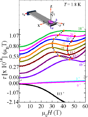
Figure 1: Measure torque ($\tau$) as a function of magnetic field for different polar angles ($\theta$) and azimuthal angle $\phi=90^{\circ}$. A peak dip structure is observed in the torque, and is seen to evolve with $\theta$. Individual torque curves have been offset for clarity. (inset: a crystal on the cantilever with the various coordinate systems: $XYZ\rightarrow$lab frame, $xyz\rightarrow$frame fixed to the cantilever, so that $X$ and $x$ coincide. $\theta$ is the angle that the normal to the crystal makes with the magnetic field, and the measured magnetic torque along the $X$-direction is referred to as $\tau$.)

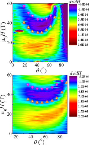
Figure 2: Derivative of experimentally measured magnetic torque with respect to field ($\frac{d\tau}{dH}$) as a function of field and angle ($\theta$) for $\phi=90^{\circ}$ (Top) and $\phi=0^{\circ}$ (Bottom) . The position of the maxima in the torque is indicated by regular triangles while that of the subsequent minima is marked by inverted triangles.

We use theoretical modeling of the non-monotonic features in the high field response to distinguish between potential microscopic models. Our starting point is the usual spin HamiltonianChaloupka et al. (2010, 2013) with nearest-neighbor Kitaev and Heisenberg interactions:

$$J_{\rm{h}}\sum_{<ij>}\overrightarrow{\sigma_{i}}.\overrightarrow{\sigma_{j}}+J_{\rm{K}}\sum_{<ij>}\sigma_{i}^{\gamma}\sigma_{j}^{\gamma}$$ (1)

where $\gamma=x,y,z$ labels an axis in spin space and a bond direction of the honeycomb lattice. Model A is parametrised by nearest-neighbour interactions $J_{\rm{h}}<0$ and $J_{\rm{K}}>0$. In Model B, further neighbor antiferromagnetic Heisenberg couplings $J_{2}$ and $J_{3}$ Kimchi and You (2011) are introduced up to the third nearest neighbor, with $J_{\rm{h}}>0$ and $J_{\rm{K}}<0$. In Model C, bond-dependent nearest-neighbor symmetric off-diagonal terms $H_{\rm{od}}^{(\gamma)}=\Gamma\sum_{\alpha\neq\beta\neq\gamma}\sum_{\{i,j\}}(\sigma_{i}^{\alpha}\sigma_{j}^{\beta}+\sigma_{i}^{\beta}\sigma_{j}^{\alpha})$ (where $\alpha$ and $\beta$ are the two remaining directions apart from the Kitaev bond direction $\gamma$) Rau et al. (2014) and $H_{\rm{od}}^{\prime}=\Gamma^{\prime}\sum_{\alpha\neq\beta\neq\gamma}\sum_{\{i,j\}}(\sigma_{i}^{\beta}\sigma_{j}^{\gamma}+\sigma_{i}^{\gamma}\sigma_{j}^{\beta}+\sigma_{i}^{\alpha}\sigma_{j}^{\gamma}+\sigma_{i}^{\gamma}\sigma_{j}^{\alpha})$ Rau and Kee (2014) accounting for trigonal distortions of the oxygen octahedra, are introduced. The main features of these models are summarized in Table I.

For our calculations, we use a hexagonal 24-site cluster Chaloupka et al. (2013, 2010); Rau et al. (2014); Rau and Kee (2014) with periodic boundary conditions. The effect of the applied field $\overrightarrow{H}=H\hat{z}$ (in the lab frame) on the system is described by $H_{\rm{mag}}=(\frac{g}{2})\sum_{i}\sum_{\gamma}h_{\gamma}\sigma_{i}^{\gamma}$, with $g\approx 1.78$ Chaloupka et al. (2013) and $\overrightarrow{h}=(h_{x},h_{y},h_{z})$ being the field as expressed in the crystal octahedron frame. Exact diagonalization calculations for the ground state energy and eigenvector were performed using a Modified Lanczos algorithmGagliano et al. (1986) (for details see SI). The code was benchmarked by reproducing the results in Chaloupka et al. (2013). The chosen parameters were verified to be consistent with the zigzag ground state of Na₂IrO₃ by calculating structure factors $S(\overrightarrow{Q)}$ Rau et al. (2014); Rau and Kee (2014); Yadav et al. (2016)(see SI).

Model	$J_{h}$	$J_{K}$	$J_{2}$	$J_{3}$	$\Gamma$	$\Gamma^{\prime}$
Antiferromagnetic Kitaev (Model A)	-	+	$\times$	$\times$	$\times$	$\times$
Ferromagnetic Kitaev (Model B)	+	-	+	+	$\times$	$\times$
Ferromagnetic Kitaev (Model C)	+	-	$\times$	$\times$	+	-

Table 1: Models considered for exact diagonalisation calculations, where $J_{h}$ refers to the nearest-neighbor Heisenberg interaction, $J_{K}$ refers to the Kitaev interaction, $J_{2}$ and $J_{3}$ refer to further-neighbor Heisenberg terms, and $\Gamma$ and $\Gamma^{\prime}$ refer to symmetric off-diagonal exchange interactions.

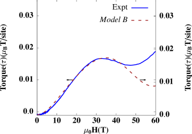
Figure 3: Torque as a function of magnetic field (in $\mu_{B}$ tesla per site) for Model B (denoted by $\tau_{B}$) with parameters $J_{\rm{h}}=3.6$, $J_{\rm{K}}=-30.0$ (in meV),corresponding to the orientation $\theta=42^{\circ}$, $\phi=0^{\circ}$. In this case, further neighbor interactions $J_{2}=0.6$, $J_{3}=1.8$ (in meV) are necessary to stabilize a zigzag ground state. The experimental data (solid line) for this orientation is plotted along with the torque response (dashed line) calculated for this model for comparison.

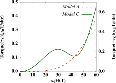
Figure 4: Magnetic torque calculated as a function of magnetic field (in $\mu_{B}$ tesla per site) for Model A (denoted by $\tau_{A}$) with parameters $J_{\rm{h}}=-4.0$, $J_{\rm{K}}=21.0$ (in meV), corresponding to the orientation $\theta=36^{\circ}$, $\phi=0^{\circ}$, and for Model C (denoted by $\tau_{C}$) with parameters $J_{\rm{h}}=4.0$, $J_{\rm{K}}=-16.0,$ $\Gamma=2.4$, $\Gamma^{\prime}=-3.2$ (in meV), corresponding to the same orientation. In Model A (dashed line) characterized by a stable zigzag phase, no peak-dip feature appears, unlike experimental observations. In contrast, in Model C (solid line), where a fine-tuned zigzag phase requires the introduction of nearest-neighbor anisotropic terms $\Gamma$ and $\Gamma^{\prime}$, the magnetic field dependence of magnetic torque shows a peak-dip feature corresponding with experiment.

The calculated torque responses for the different models are shown in Figures 3 and 4. We find that the peak-dip feature in the torque response is reproduced only by Models B $\&$ C), whereas Model A displays a monotonic increase in the magnetic torque with magnetic field. We have performed exact diagonalization simulations for magnetic fields up to 300 T for Model A (for the parameters used in Fig. 4), and found a single peak in the torque response at a field slightly lower than 150 T, beyond which it decreases with increase in field strength and no further features are observed. We have also considered variants of Model A with isotropic $J_{2}$ and $J_{3}$ as well as anisotropic $\Gamma$ and $\Gamma^{\prime}$ terms, and have confirmed the absence of any peak-dip features even with such additional terms present (please refer to Table I in the SI for a summary of the different variants considered).

Our results strongly indicate that Na₂IrO₃ is described by a model dominated by a ferromagnetic Kitaev exchange. The distinctive peak-dip feature in the torque response provides an independent handle for constraining experimental data. We note that classical Monte Carlo simulations were unable to reproduce the feature, underlining the importance of quantum effects in this material, as has also been emphasized in the recent literature Janssen et al. (2017). Of the two types of ferromagnetic Kitaev exchange models we consider, in Model B, the peak-dip feature is observed over a large parameter range, while in Model C, it only appears upon inclusion of a significant $\Gamma^{\prime}<0$ term, which is physically associated with trigonal distortion in Na₂IrO₃. The inclusion of significant anisotropy terms in Model B does not yield additional peak-dip features, and the feature survives only for relatively small values of additional anisotropic interactions. Models B and C can thus potentially be distinguished by high field torque magnetometry measurements on chemically doped Na₂IrO₃ with various extents of trigonal distortion.

We compute the evolution of the spin correlation functions with distance for increasing magnetic field values. The extent of decay of the correlation functions with distance reveals the presence or absence of long range correlations in the high field regime. The correlation functions $C_{ij}=<(\overrightarrow{\sigma_{i}}-<\overrightarrow{\sigma_{i}}>).(\overrightarrow{\sigma_{j}}-<\overrightarrow{\sigma_{j}}>)>$ are calculated for a chosen set of neighboring sites in the 24-site cluster, and plotted in Fig. 5 as a function of $\frac{|i-j|}{a}$ ($a$ being the distance between nearest neighbor sites) for different values of the applied magnetic field. We find that the decay of the correlation functions is much faster at relatively higher values of the applied field, and the amplitude of their oscillation falls off rapidly with increasing fields, in particular above the zigzag ordering scale. Furthermore, structure factor calculations do not show a crossover from antiferromagnetic zigzag order to any of the known ordered states at the position of the metamagnetic transition manifested through the peak-dip in the transverse magnetization. Indications are therefore that the high field regime beyond the peak-dip feature manifests spin-liquid physics in Na₂IrO₃.

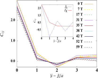
Figure 5: The correlation functions $C_{ij}$ calculated as a function of $\frac{|i-j|}{a}$, $a$ being the distance between two neighboring sites, with parameters $J_{\rm{h}}=4.0$, $J_{\rm{K}}=-16.0$, $\Gamma=2.4$, $\Gamma^{\prime}=-3.2$ (in meV), for an orientation of $\theta=36^{\circ}$, $\phi=0^{\circ}$. The inset shows the corresponding plots for a pure Heisenberg model with $J_{\rm{h}}=16.0$ meV(blue) and a pure Kitaev model with $J_{\rm{K}}=-16.0$ meV(red). It can be clearly seen that for higher fields(>30 T), the correlation functions fall rapidly with distance, signalling spin-liquid physics.

Our work sheds light on the universality of field-induced spin liquid physics in Kitaev systems, which we find to be signalled by a peak dip structure in the anisotropic magnetisation at the zigzag ordering scale both in Na₂IrO₃ and $\alpha-$RuCl₃ Sears et al. (2017); Yadav et al. (2016); Zheng et al. (2017); Hirobe et al. (2017); Johnson et al. (2015). Recent calculations of thermal Hall effect in $\alpha-$RuCl₃ Cookmeyer and Moore (2018) as well as electron energy loss spectroscopy experiments Koitzsch et al. (2017) also favour a dominant ferromagnetic Kitaev model. The striking similarities between these two materials indicates that the experimental features in the magnetoresponse that we report here are governed by intrinsic Kitaev physics, and not peculiarities associated with parameters beyond the scope of our model such as interlayer couplings and disorder characteristics, expected to be very different for these two materials. The microscopic models we calculate here are thus indicated to be relevant to a broad class of honeycomb Kitaev materials for exploring a field-induced spin liquid phase.

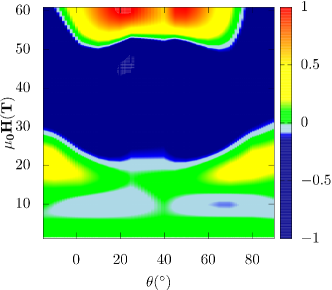
Figure 6: The figure shows a calculated contourplot of $\frac{d\tau}{dH}$ in the $\theta-H$ plane, for parameters $J_{\rm{h}}=3.6$, $J_{\rm{K}}=-18.0$, $J_{2}=2.4$ and $J_{3}=1.8$ (in meV), i.e. Model B, corresponding to the azimuthal angle $\phi=20^{\circ}$. We find that the position of the peak-dip feature, indicated by the regions where $\frac{d\tau}{dH}$ changes sign, shifts closer to the origin for increasing(decreasing) values of the polar angle $\theta$ for $\theta$ close to $0^{\circ}$ ($90^{\circ}$), in agreement with the experimental results. At the extreme values of $\theta$, the width of the region of nonmonotonicity increases, at variance with experiment. The torque values obtained in our simulations can be negative, and in such cases we plot $-\frac{d\tau}{dH}$ instead.

The authors gratefully acknowledge useful discussions with Giniyat Khaliullin, Itamar Kimchi, Subhro Bhattacharjee and Steve Winter. We thank E. V. Sampathkumaran for the generous use of facilities for crystal growth. VT acknowledges DST for a Swarnajayanti grant (No. DST/SJF/PSA-0212012-13). SDD and SES acknowledge support from the Royal Society, the Winton Programme for the Physics of Sustainability, and the European Research Council under the European Unions Seventh Framework Programme (grant number FP/2007-2013)/ERC Grant Agreement number 337425. LB is supported by DOE-BES through award DE-SC0002613. GC acknowledges the support of the US National Science Foundation via grant DMR 1712101. AM acknowledges the support of the HFML-RU/FOM, member of the European Magnetic Field Laboratory(EMFL). HYK acknowledges the support of the NSERC of Canada and the center for Quantum Materials at the University of Toronto.

High field experiments were performed by S.D.D. with contributions from Z.Z., E.M., R.D.M., G.L., L.B. and A.M.. Theory was developed and calculations performed by S.K. and V.T. with contributions from H.Y.K. and J.G.R. Single crystal growth was performed by S.D.D. and G.C. The project was conceived and supervised by S.E.S. and V.T. The manuscript was written by S.D.D., S.K., V.T., and S.E.S. with inputs from all the authors.

Sitikantha D. Das^1,11 Sarbajaya Kundu² Zengwei Zhu³ Now at: ]National High Magnetic Field Center and School of Physics, Huazhong University of Science and Technology, Wuhan 430074, China Eundeok Mun³ Now at: ]Department of Physics, Simon Fraser University, Burnaby, BC, Canada V5A-1S6 Ross D. McDonald³ Gang Li⁴ Now at: ]Department of Physics, University of Michigan, 500 S State St, Ann Arbor, MI 48109, USA Luis Balicas⁴ Now at: ]Institute of Physics, Chinese Academy of Sciences, P.O Box 603, Beijing 100190, China Alix McCollam⁵ Gang Cao^6,7 Jeffrey G. Rau⁸ Hae-Young Kee^9,10 Vikram Tripathi² Suchitra E. Sebastian¹

A1. Experimental details

Crystals of Na₂IrO₃ about 100 micron along a side were prepared using Na₂CO₃ slightly in excess Singh and Gegenwart (2010). The insulating nature of the sample was confirmed using four-probe resistivity measurements. Magnetization measurements were performed using a Quantum Design SQUID magnetometer upto a field of 5 tesla, and these showed the presence of an antiferromagnetic transition around $T_{N}\sim$15 K, below which the system orders into a zigzag phase Choi et al. (2012); Ye et al. (2012); Liu et al. (2011). A linear Curie-Weiss fit to the high temperature inverse susceptibility data gives an effective Ir moment $\mu_{eff}=1.67\mu_{B}$ and Curie temperature $\theta_{p}=-116$ K. This gives a frustration index $\frac{\theta_{p}}{T_{N}}\sim 8$, which is in agreement with the results obtained from other groups.

The torque ($\overrightarrow{\tau}=\overrightarrow{m}\times\overrightarrow{B}$) was measured using a PRC 120 piezoresistive cantilever at the pulsed field facility at the National High Magnetic Field Laboratory, Los Alamos. The crystal was mounted on the cantilever with vacuum grease. The cantilever assembly was mounted on a sample holder made of G-10 and capable of rotation about the magnetic field axis. The pulse duration was 25 ms. All the angles ($\theta$) were measured with respect to the normal to the flat surface of the crystal (which is the nominal c-axis) and the magnetic field $H$. For each value of $\theta$ the torque response was measured for the increasing and decreasing cycles of the pulse which had a high degree of overlap ruling out significant magneto-caloric effects which might become evident in pulsed field measurements. Further measurements were performed for various in-planar orientations $\phi$ of the crystal. The torque response for a second crystal from an independently grown batch, mentioned in the main text, is shown in Fig. 8.

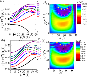
Figure 7: Torque as a function of magnetic field($H$) measured independently for a second crystal corresponding to two different in-plane orientations $\phi$ separated by $90^{\circ}$, is shown in (a) and (b), and is again found to show nonmonotonous behavior for a range of orientations. The corresponding plots for $\frac{d\tau}{dH}$ as a function of $H$ are shown in (c) and (d). $\theta$ is the angle that the normal to the crystal makes with the magnetic field, and is defined in the main text.

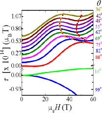
Figure 8: Torque ($\tau$) as a function of magnetic field for different angular orientations ($\theta$) and $\phi=0^{\circ}$ corresponding to the first crystal as mentioned in the main text.

A2. Numerical setup and Exact Diagonalization algorithm

Figure 9: Our 24-site fragment with periodic boundary conditions

The N lattice sites were numbered 0,1,2…N-1 (for N=24), and specific pairs of these sites were identified as ‘bonds’ or ‘links’, of type $x$, $y$ or $z$. Every site has a spin with two possible states $|1>$ or $|0>$. The system then has $2^{N}$ configurations or underlying basis states, where each configuration is denoted by $|s_{N-1},s_{N-2}...s_{0}>$ with $s_{i}=0,1$. Corresponding to such a set of binary numbers, we have a decimal equivalent given by $|s_{N-1}{\rm{x}2^{N-1}+s_{N-2}{\rm{x}2^{N-2}+...s_{0}{\rm{x}2^{0}>}}}$. The basis vectors were thus denoted as $|0>$, $|1>$…$|2^{N-1}>$. An arbitrary state vector $|\psi>$ can be expanded in terms of these basis vectors as $|\psi>=\sum_{i=0}^{2^{N-1}}a_{i}|i>$. The ground state $\Psi_{0}$ for this Hamiltonian $H_{0}$ was determined using the Modified Lanczos algorithm.

The Modified Lanczos algorithm Gagliano et al. (1986) requires the initial selection of a trial vector $\psi_{0}$ (constructed using a random number generator in our case) which should have a nonzero projection on the true ground state of the system in order for the algorithm to converge properly. A normalized state $\psi_{1}$, orthogonal to $\psi_{0}$, is defined as

$$\psi_{1}=\frac{H_{0}\psi_{0}-<H_{0}>\psi_{0}}{\sqrt{<H_{0}^{2}>-<H_{0}>^{2}}}$$ (2)

In the basis $\{\psi_{0},\psi_{1}\}$, $H_{0}$ has a 2x2 representation which is easily diagonalized. Its lowest eigenvalue and corresponding eigenvector are better approximations to the true ground state energy and wavefunction than the quantities $<H_{0}>$ and $\psi_{0}$ considered initially. The improved energy and wavefunction are given by

$$\epsilon=<H_{0}>+b\alpha$$ (3)

and

$$\tilde{\psi_{0}}=\frac{\psi_{0}+\alpha\psi_{1}}{\sqrt{1+\alpha^{2}}}$$ (4)

where $b=\sqrt{<H_{0}^{2}>-<H_{0}>^{2}}$, $f=\frac{<H_{0}^{3}>-3<H_{0}><H_{0}^{2}>+2<H_{0}>^{3}}{2b^{3}}$ and $\alpha=f-\sqrt{1+f^{2}}$. The method can be iterated by considering $\tilde{\psi_{0}}$ as a new trial vector and repeating the above steps. The Modified Lanczos method helps in obtaining a reasonably good approximation to the actual ground state of the system while storing only three vectors, $\psi_{0}$, $H_{0}\psi_{0}$ and $H_{0}^{2}\psi_{0}$ rather than the entire Hamiltonian in the spin basis representation. This is especially advantageous as the number of basis vectors increases rapidly with the number of spin sites. In the regular Lanczos algorithm, the matrix is first reduced to a tridiagonal form before computing the ground state eigenvector. However, there can be issues with the convergence to the true ground state because of loss of orthogonality among the vectors. This is circumvented in this algorithm as orthogonality is enforced at each and every step of the iteration.

After the determination of the ground state $\Psi_{0}$ to a reasonable approximation, the magnetization $\vec{m}_{|\psi>}$ was obtained in this state with components ($m_{x},m_{y},m_{z}$), where $m_{\gamma}=<\psi|\sum_{i=0}^{N-1}\sigma_{i}^{\gamma}|\psi>$, and was transformed to the lab frame from the octahedral frame, the components in the lab frame being ($m_{X},m_{Y},m_{Z}$). Finally, in the lab frame, torque $\Gamma_{X}=m_{Y}H$.

A3. Coordinate system transformations

For our exact diagonalization calculations, we have transformed the external magnetic field from the laboratory frame to the $\rm{IrO}_{6}$ octahedral frame by defining intermediate crystal and cantilever axes, and transformed the calculated magnetization back from this frame to the lab frame. We explain the transformations used in the following:

Notations:

Laboratory axes: $\hat{X},\hat{Y},\hat{Z}$

Cantilever axes: $\hat{x,}\hat{y},\hat{z}$

Crystal axes: $\hat{a},\hat{b},\hat{c}$

Octahedral axes: $\hat{p},\hat{q},\hat{r}$

Laboratory to cantilever axes:

The lab $\hat{X}$-axis and the cantilever $\hat{x}$-axis are always coincident. Let $\theta$ be the angle between the $\hat{Z}$ and $\hat{z}$ axes.We have

$$|\hat{x}\hat{y}\hat{z}>=M_{Lab\rightarrow Canti}|\hat{X}\hat{Y}\hat{Z}>$$

$$|\hat{X}\hat{Y}\hat{Z}>=L_{Canti\rightarrow Lab}|\hat{x}\hat{y}\hat{z}>$$

where

$$M_{Lab\rightarrow Canti}=\left(\begin{array}[]{ccc}1&0&0\\ 0&\cos\theta&-\sin\theta\\ 0&\sin\theta&\cos\theta\end{array}\right)$$

$$L_{Canti\rightarrow Lab}=\left(\begin{array}[]{ccc}1&0&0\\ 0&\cos\theta&\sin\theta\\ 0&-\sin\theta&\cos\theta\end{array}\right)$$

Cantilever to crystal axes:

The honeycomb layer formed by the Ir atoms resides on the crystallographic $ab$ plane. Let the $\hat{a}$-axis of the crystal make an angle $\phi$ with the $\hat{x}$-axis of the cantilever. Then,

$$|\hat{a}\hat{b}\hat{c}>=M_{Canti\rightarrow Crystal}|\hat{x}\hat{y}\hat{z}>$$

$$|\hat{x}\hat{y}\hat{z}>=L_{Crystal\rightarrow Canti}|\hat{a}\hat{b}\hat{c}>$$

$$M_{Canti\rightarrow Crystal}=\left(\begin{array}[]{ccc}\cos\phi&\sin\phi&0\\ -\sin\phi&\cos\phi&0\\ 0&0&1\end{array}\right)$$

$$L_{Crystal\rightarrow Canti}=\left(\begin{array}[]{ccc}\cos\phi&-\sin\phi&0\\ \sin\phi&\cos\phi&0\\ 0&0&1\end{array}\right)$$

Crystal to octahedral axes:

Since the [111] direction in the octahedral frame is perpendicular to the honeycomb lattice, the unit vectors are related as follows:

$$\hat{c}=\frac{\hat{p}+\hat{q}+\hat{r}}{\sqrt{3}}$$

$$\hat{b}=\frac{-\hat{p}+\hat{q}}{\sqrt{2}}$$

$$\hat{a}=\frac{\hat{p}+\hat{q}-2\hat{r}}{\sqrt{6}}$$

Then,

$$|\hat{p}\hat{q}\hat{r}>=M_{Crystal\rightarrow Octa}|\hat{a}\hat{b}\hat{c}>$$

$$|\hat{a}\hat{b}\hat{c}>=L_{Octa\rightarrow Crystal}|\hat{p}\hat{q}\hat{r}>$$

$$M_{Crystal\rightarrow Octa}=\left(\begin{array}[]{ccc}\frac{1}{\sqrt{6}}&-\frac{1}{\sqrt{2}}&\frac{1}{\sqrt{3}}\\ \frac{1}{\sqrt{6}}&\frac{1}{\sqrt{2}}&\frac{1}{\sqrt{3}}\\ -\sqrt{\frac{2}{3}}&0&\frac{1}{\sqrt{3}}\end{array}\right)$$

$$L_{Octa\rightarrow Crystal}=\left(\begin{array}[]{ccc}\frac{1}{\sqrt{6}}&\frac{1}{\sqrt{6}}&-\sqrt{\frac{2}{3}}\\ -\frac{1}{\sqrt{2}}&\frac{1}{\sqrt{2}}&0\\ \frac{1}{\sqrt{3}}&\frac{1}{\sqrt{3}}&\frac{1}{\sqrt{3}}\end{array}\right)$$

Lab to octahedral and octahedral to lab frame:

Let the components of the magnetic field be $(0,0,H)$ in the lab frame and $(h_{p},h_{q},h_{r})$ in the octahedral frame. Then

$$|h_{p}h_{q}h_{r}>=M_{Crystal\rightarrow Octa}M_{Canti\rightarrow Crystal}M_{Lab\rightarrow Canti}|00H>$$

which finally gives us

$$h_{p}=(-\frac{1}{\sqrt{6}}\sin\theta\sin\phi+\frac{1}{\sqrt{2}}\sin\theta\cos\phi+\frac{1}{\sqrt{3}}\cos\theta)H$$

$$h_{q}=(-\frac{1}{\sqrt{6}}\sin\theta\sin\phi-\frac{1}{\sqrt{2}}\sin\theta\cos\phi+\frac{1}{\sqrt{3}}\cos\theta)H$$

$$h_{r}=(\sqrt{\frac{2}{3}}\sin\theta\sin\phi+\frac{1}{\sqrt{3}}\cos\theta)H$$

Let the components of the magnetization vector $\overrightarrow{m}$ be $(m_{X},m_{Y},m_{Z})$ in the lab frame and $(m_{p},m_{q},m_{r})$ in the octahedral frame. Then,

$$|m_{X}m_{Y}m_{Z}>=L_{Canti\rightarrow Lab}L_{Crystal\rightarrow Canti}L_{Octa\rightarrow Crystal}|m_{p}m_{q}m_{r}>$$

from where we find

$$m_{Z}=(-\frac{m_{p}}{\sqrt{6}}-\frac{m_{q}}{\sqrt{6}}+m_{r}\sqrt{\frac{2}{3}})\sin\theta\sin\phi+\frac{m_{p}-m_{q}}{\sqrt{2}}\sin\theta\cos\phi+\frac{(m_{p}+m_{q}+m_{r})}{\sqrt{3}}\cos\theta$$

and

$$m_{Y}=(\frac{m_{p}}{\sqrt{6}}+\frac{m_{q}}{\sqrt{6}}-m_{r}\sqrt{\frac{2}{3}})\cos\theta\sin\phi+\frac{(-m_{p}+m_{q})}{\sqrt{2}}\cos\theta\cos\phi+\frac{(m_{p}+m_{q}+m_{r})}{\sqrt{3}}\sin\theta$$

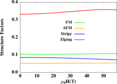
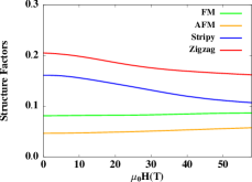
(a)(b) (c)

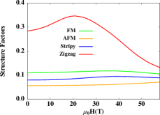
Figure 10: Evolution of structure factors for different ordered phases as a function of the field for (a) $J_{h}=3.2$, $J_{\rm{K}}=-12$, $J_{2}=4$, $J_{3}=2$(in meV), (b) $J_{h}=1.6$, $J_{\rm{K}}=-16.0$, $J_{2}=1.2$ and $J_{3}=0.8$(in meV), and (c) $J_{h}=4.0$, $J_{\rm{K}}=-16.0$, $\Gamma=2.4$ and $\Gamma^{\prime}=-3.2$(in meV).

A4. Structure factor calculations

To determine different phases of the system in the presence of an applied magnetic field, one needs to calculate the adapted structure factors acting as order parameters trousselet2011effects. The corresponding dominant order wavevectors $\overrightarrow{Q}=\overrightarrow{Q_{max}}$ characterize the nature of the magnetic ordering in various field regimes. The static structure factors $S(\overrightarrow{Q})$ for different spin configurations are given by

$$S_{zigzag}^{\gamma}=\frac{1}{N^{2}}\sum_{r,r^{\prime},\beta,\beta^{\prime}}\exp[i\overrightarrow{Q_{\gamma}.}(\overrightarrow{r^{\prime}}-\overrightarrow{r})]\nu_{\beta,\beta^{\prime}}(<\overrightarrow{\sigma_{r,\beta}}.\overrightarrow{\sigma_{r^{\prime},\beta^{\prime}}}>-\sum_{\gamma}<\sigma_{r,\beta}^{\gamma}><\sigma_{r^{\prime},\beta^{\prime}}^{\gamma}>)$$ (5)

$$S_{Neel}=\frac{1}{N^{2}}\sum_{r,r^{\prime},\beta,\beta^{\prime}}\nu_{\beta,\beta^{\prime}}(<\overrightarrow{\sigma_{r,\beta}}.\overrightarrow{\sigma_{r^{\prime},\beta^{\prime}}}>-\sum_{\gamma}<\sigma_{r,\beta}^{\gamma}><\sigma_{r^{\prime},\beta^{\prime}}^{\gamma}>)$$ (6)

$$S_{FM}=\frac{1}{N^{2}}\sum_{r,r^{\prime},\beta,\beta^{\prime}}(<\overrightarrow{\sigma_{r,\beta}}.\overrightarrow{\sigma_{r^{\prime},\beta^{\prime}}}>-\sum_{\gamma}<\sigma_{r,\beta}^{\gamma}><\sigma_{r^{\prime},\beta^{\prime}}^{\gamma}>)$$ (7)

$$S_{stripy}^{\gamma}=\frac{1}{N^{2}}\sum_{r,r^{\prime},\beta,\beta^{\prime}}\exp[i\overrightarrow{Q_{\gamma}.}(\overrightarrow{r^{\prime}}-\overrightarrow{r})](<\overrightarrow{\sigma_{r,\beta}}.\overrightarrow{\sigma_{r^{\prime},\beta^{\prime}}}>-\sum_{\gamma}<\sigma_{r,\beta}^{\gamma}><\sigma_{r^{\prime},\beta^{\prime}}^{\gamma}>)$$ (8)

where each site is labeled by an index $i$ and a position in the unit cell $\overrightarrow{r}$ ,$\beta$ denotes the sublattice index($\beta=A,B$), and $\gamma=x,y$ or $z$. The contribution to the structure factors coming from the alignment of the spins with the field direction has explicitly been deducted in this definition. The structure factors for the four different phases are plotted as a function of field for different models in Fig. 10, which clearly shows that AFM zigzag is the dominant spin configuration in all cases.

A5. Magnetization as a function of field

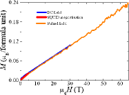
(a)(b)

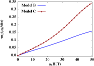
Figure 11: (a) Isotropic magnetization measured using an extraction magnetometer in pulsed magnetic fields, and using a force magnetometer in DC fields, shows no features up to 60 T, calibration is performed using magnetization measurements on a pellet of sodium iridate in a SQUID magnetometer, (b) Isotropic magnetization $m_{Z}$ (in $\mu_{B}$ per atom) calculated as a function of field, for model B with $J_{h}=2.4$, $J_{{\rm{K}}}=-12.0$, $J_{2}=1.6$, $J_{3}=1.2$(in meV) for the orientation $\theta=18^{\circ}$, $\phi=90^{\circ}$, and for model C with $J_{h}=4.0$, $J_{{\rm{K}}}=-16.0$, $\Gamma=2.4$ and $\Gamma^{\prime}=-3.2$(in meV), for the orientation $\theta=36^{\circ}$, $\phi=0^{\circ}$.

The isotropic magnetization($m_{Z}$) was measured using an extraction magnetometer in pulsed magnetic fields up to 60 T and calibrated to obtain $m_{Z}$ per site using force magnetometry measurements in steady magnetic fields, and magnetization measurements in a SQUID magnetometer. It is found to be largely featureless and increases linearly with field up to 60 T. We have determined the behavior of $m_{Z}$ per site numerically for different relevant models and the results, along with the experimental curves, are shown in Fig. 11 .

A6. Extended modelling

.1 Observation of peak dip feature for some more orientations:

Here we consider models B and C of the main text and show the existence of the peak-dip feature in the torque response for different combinations of polar and azimuthal angles. This is illustated in figures 12 and 13 for models B and C respectively.

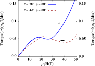
(a)(b)

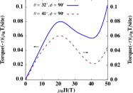
Figure 12: Calculated values of torque for model B with parameters $J_{h}=2.4$, $J_{k}=-12.0$, $J_{2}=1.6$, $J_{3}=1.2$ (in meV) for different polar and azimuthal angles as indicated in the figures. A robust peak-dip feature is observed for a wide range of orientations in model B. (See also the contourplot in Fig.6 of the main text.)

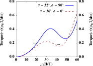
(a)(b)

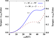
Figure 13: Calculated values of torque for model C with parameters $J_{h}=4.0$, $J_{k}=-16.0$, $\Gamma=2.4$, $\Gamma^{\prime}=-3.2$ (meV) for different polar and azimuthal angles as indicated in the figure. In (b) the peak-dip feature is present but is shallower than that observed in (a).

.2 General absence of a peak-dip feature in models with an antiferromagnetic Kitaev interaction ($J_{K}>0$):

The purpose of this section is to show that models with an antiferromagnetic sign of the Kitaev coupling tuned to a zigzag ground state by a variety of subleading interactions are generally unable to produce the peak-dip feature in the torque that is observed in experiment. Figures 14 and 17 illustrate this for models with additional $\Gamma$ and $\Gamma^{\prime}$ interactions, and figures 15 and 16 for models with various combinations of antiferromagnetic as well as ferromagnetic further neighbour interactions $J_{2}$ and $J_{3}$. The different combinations of parameters considered is summarized in Table I.

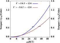
(a)(b)

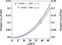
Figure 14: Calculated values of the torque for models with $J_{h}=-8.0$, $J_{k}=40.0$(meV), for the orientation $\theta=36^{\circ}$, $\phi=0^{\circ}$, with $\Gamma$ and $\Gamma^{\prime}$ values as indicated in the figures. We observe that additional $\Gamma$ and $\Gamma^{\prime}$ terms do not give rise to any peak-dip features in the torque response.

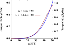
(a)(b)

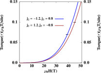
Figure 15: Here we demonstrate the calculated torque response for different models with a ferromagnetic Heisenberg and antiferromagnetic Kitaev interaction with further neighbor Heisenberg interactions. (a) and (b) correspond to $J_{h}=-4.0$, $J_{k}=21.0$ (meV) for the orientation $\theta=48^{\circ}$, $\phi=90^{\circ}$, for $J_{2}$ and $J_{3}$ interactions as indicated in the figure. We observe that further neighbour interactions $J_{2}$ and $J_{3}$ do not give rise to any peak-dip features in the torque response.

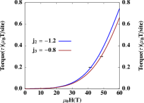
(a)(b)

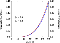
Figure 16: Here, we have considered combinations of parameters for $J_{h}=-4.0$, $J_{K}=21.0$ (in meV) with either $J_{2}$ or $J_{3}$ terms present but not both. In (a), we consider $J_{2}$ or $J_{3}$ which is ferromagnetic and in (b), we consider these interactions to be antiferromagnetic, both for the orientation $\theta=48^{\circ}$, $\phi=90^{\circ}$. In neither case do we see any peak-dip features in the torque response.

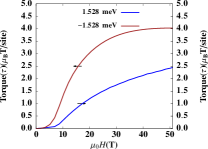
(a)(b)

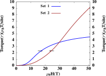
Figure 17: Here we demonstrate the calculated torque response for different models with a ferromagnetic Heisenberg and antiferromagnetic Kitaev interaction with additional anisotropic parameters.(a) corresponds to $J_{h}=-1.84$, $J_{K}=3.2$ (meV) for the orientation $\theta=69^{\circ}$, $\phi=90^{\circ}$ with an additional $\Gamma$ term taking values indicated in the figure. (b) shows the torque response for two sets of parameters with $J_{h}<0$, $J_{K}>0$ and $\Gamma>0$ at different orientations of the field. Here Set 1 corresponds to $J_{h}=-1.84$, $J_{K}=3.2$ and $\Gamma=1.528$ (meV) for $\theta=36^{\circ}$ and $\phi=0^{\circ}$, and Set 2 corresponds to $J_{h}=-12.0$, $J_{K}=17.0$, and $\Gamma=12.0$ (meV) for $\theta=48^{\circ}$ and $\phi=90^{\circ}$.

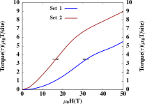
(a)(b)

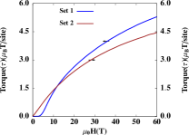
Figure 18: The figure (a) shows the calculated torque response for models with both the Kitaev and Heisenberg interactions ferromagnetic. Here Set 1 corresponds to $J_{h}=-1.0$, $J_{k}=-8.0$ and $\Gamma=4.0$ (in meV) for $\theta=48^{\circ}$ and $\phi=90^{\circ}$ while Set 2 corresponds to $J_{h}=-1.7$, $J_{K}=-6.6$, $J_{3}=2.7$ and $\Gamma=6.6$ (in meV) for $\theta=18^{\circ}$ and $\phi=90^{\circ}$. The figure (b) shows the calculated torque response for models with $|\Gamma|>|J_{K}|$ with an antiferromagnetic Kitaev and ferromagnetic Heisenberg interaction. Here, Set 1 corresponds to $J_{h}=-0.98$,$J_{K}=1.17$ and $\Gamma=3.69$ (in meV) while Set 2 corresponds to $J_{h}=-1.99$, $J_{K}=1.99$ and $\Gamma=2.83$ (in meV), both for $\theta=69^{\circ}$ and $\phi=90^{\circ}$. Clearly, none of the parameter sets with an antiferromagnetic Kitaev interaction give rise to any peak-dip features in the torque response.

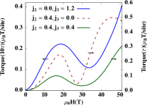
(a)(b)

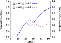
Figure 19: The calculated torque response for models with $J_{h}>0$, $J_{K}<0$ and various combinations of additional interactions $J_{2}$ and $J_{3}$. Here (a) shows the torque response for $J_{h}=2.4$, $J_{k}=-20.0$ (meV) for $\theta=36^{\circ}$ and $\phi=0^{\circ}$ with $J_{2}$ and $J_{3}$ values as indicated(in meV), and (b) shows the torque response for two sets of data where Set 1 corresponds to $J_{h}=2.4$, $J_{K}=-12.0$, $J_{2}=0.2$ and $J_{3}=0.2$ (in meV) for $\theta=32^{\circ}$ and $\phi=90^{\circ}$, while Set 2 corresponds to $J_{h}=2.4$, $J_{K}=-12.0$, $J_{2}=0.8$ and $J_{3}=0.8$ (in meV) for $\theta=41^{\circ}$ and $\phi=90^{\circ}$. We observe that peak-dip features, sometimes more than one, are observed in the expected field range for all of these models, even though most of them do not exhibit a zigzag ordered ground state. Moreover, the shift in the position of the peak-dip feature with an increase in the values of the parameters $J_{2}$ and $J_{3}$ is clearly seen in (b).

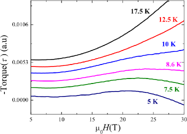
Figure 20: The figure shows the torque response corresponding to steady field measurements for $\theta=-20^{\circ}$ and $\phi=0^{\circ}$ at various temperatures in the range 5 K-17.5 K. A shallow peak-dip feature, close to around 20 T, is observed at low temperatures and no longer discernible at temperatures beyond about 12.5 K. This shows that the peak-dip feature is associated with a transition from the zigzag ordered ground state to a state with a significantly different torque response.

.3 Peak-dip features in models with a ferromagnetic Kitaev interaction ($J_{K}<0$):

Here we consider the torque response for models with a ferromagnetic Kitaev interaction where the nearest neighbour Heisenberg interaction is also ferromagnetic, with an additional anisotropic $\Gamma$ and/or isotropic $J_{3}$ interaction. Such models have been proposed in the literature for the related Kitaev material $\alpha-$RuCl₃ which also has a zigzag ground state. We did not see a peak-dip feature in such models; however, there is a slight flattening of the torque response curve at intermediate fields. This is illustrated in Fig. 18(a).

.4 Peak-dip features in the absence of zigzag order:

Here we demonstrate that models with a ferromagnetic Kitaev $J_{K}$, antiferromagnetic Heisenberg $J_{h}$ and additional antiferromagnetic further-neighbour interactions $J_{2}$ and $J_{3}$ can give rise to peak-dip features even in the absence of zigzag order in the ground state. The presence of the peak-dip features thus provides an independent handle which can distinguish the response of such models from those with an antiferromagnetic Kitaev interaction. This is illustrated in Fig. 19, where we find that the peak-dip feature is observed even for those combinations of parameters where either $J_{2}$ or $J_{3}$ vanishes, or $J_{2}$, $J_{3}$ are both small as compared to the nearest-neighbour interactions $J_{h}$ and $J_{K}$. Such combinations of parameters often do not give rise to a zigzag ordered ground state, and cannot be used to represent Na₂IrO₃, but they still do give rise to prominent peak-dip features in the torque. Table 3 summarizes the different models we have considered, with a ferromagnetic Kitaev interaction and additional subdominant terms.

Model A variant	$\Gamma$	$\Gamma^{\prime}$	$J_{2}$	$J_{3}$	Ref.(if any)
1. With $\Gamma,\Gamma^{\prime}$	+	-	$\times$	$\times$	Rau and Kee (2014)
	-	+	$\times$	$\times$	Rau and Kee (2014)
	-	-	$\times$	$\times$	Rau and Kee (2014)
2. With $J_{2},J_{3}$	$\times$	$\times$	+	+
	$\times$	$\times$	-	-
	$\times$	$\times$	+	-
	$\times$	$\times$	-	+
	$\times$	$\times$	-	$\times$
	$\times$	$\times$	$\times$	-
	$\times$	$\times$	+	$\times$
	$\times$	$\times$	$\times$	+
3. With $\Gamma$	+	$\times$	$\times$	$\times$	Janssen et al. (2017),Rau et al. (2014)
	-	$\times$	$\times$	$\times$	Janssen et al. (2017),Rau et al. (2014)

Table 2: For model A ($J_{h}<0$, $J_{K}>0$), introduction of various additional terms $\Gamma$,$\Gamma^{\prime}$, $J_{2}$ and $J_{3}$, with a zigzag ground state, does not reveal any peak-dip features. The + and - indicate the sign of the coupling and $\times$ denotes the absence of the corresponding coupling. Thus, for a wide variety of parameters, antiferromagnetic Kitaev couplings do not produce the observed peak-dip feature.

	$J_{h}$	$J_{2}$	$J_{3}$	$\Gamma$	$\Gamma^{\prime}$	Peak-dip(present/absent)
Model B	+	+	+	$\times$	$\times$	Yes
	+	+	$\times$	$\times$	$\times$	Yes
	+	$\times$	+	$\times$	$\times$	Yes
Model C	+	$\times$	$\times$	+	-	Yes
Ref.Janssen et al. (2017)	-	$\times$	+	+	$\times$	No
	-	$\times$	$\times$	+	$\times$	No

Table 3: For models with $J_{K}<0$ (model B, model C as well as other models with various anisotropic and Heisenberg interactions),with a zigzag ground state, the peak-dip feature may or may not be present. The + and - indicate the sign of the coupling and $\times$ denotes the absence of the corresponding coupling. The last two sets of parameters have been suggested in Ref. Janssen et al. (2017) and correspond to a ferromagnetic Heisenberg interaction. The remaining ones correspond to an antiferromagnetic Heisenberg interaction. Clearly, the presence of zigzag order in models with $J_{K}<0$ does not necessarily produce the peak-dip feature. Thus, the peak-dip feature is an independent tool to constrain the parameter space of possible effective Hamiltonians.

.5 Evolution of the peak-dip feature as a function of polar angle $\theta$ and field $H$:

Here we discuss the evolution of the torque response for model B as a function of the polar angle $\theta$ and field value $H$, by presenting a contourplot of the first derivative of the torque, $\frac{d\tau}{dH}$ (for the torque $\tau$ and field $H$), and compare our results with the experimental data in Fig.2 of the main text. We find that for model B, a peak-dip feature is robustly observed for all orientations $\theta$ for a given value of the azimuthal angle $\phi$, and the position as well as the shape of the peak-dip evolves as a function of $\theta$, as expected from the experiment. Theoretically, the transverse magnetization (torque) response could well be negative, and in such cases, we plot $-\frac{d\tau}{dH}$ instead, as we are not interested in the absolute value of the torque obtained, but only in the position of the peak-dip, which is indicated by the regions where the first derivative of the torque changes sign. Fig.6 in the main text illustrates our results, and it is clear that although there is qualitative agreement with the experimental results, unlike the actual data, the distance between the peak and the dip, i.e. the width of the region of nonmonotonicity increases at extreme values of $\theta$.

A7: Temperature-dependence of the torque response

The torque response was measured capacitively for different temperatures in the range 5 K-17.5 K, at steady fields up to 30 T for the orientation $\theta=-20^{\circ}$, $\phi=0^{\circ}$. A peak-dip feature observed close to about 20 T at low temperatures becomes indiscernible beyond a temperature of about 12.5 K. This is illustrated in Fig. 20. The exact detection of the temperature at which this feature disappears is limited by the resolution of the measurement, as well as temperature resolution very close to the zigzag ordering temperature. Our results do however establish that the peak-dip feature is present only below the zigzag ordering temperature and is therefore related to a transition from the long-range ordered ground state.

References

- Chaloupka et al. (2010) J. Chaloupka, G. Jackeli, and G. Khaliullin, Physical Review Letters 105, 027204 (2010).
- Kimchi and You (2011) I. Kimchi and Y.-Z. You, Physical Review B 84, 180407 (2011).
- Katukuri et al. (2014) V. M. Katukuri, S. Nishimoto, V. Yushankhai, A. Stoyanova, H. Kandpal, S. Choi, R. Coldea, I. Rousochatzakis, L. Hozoi, and J. van den Brink, New Journal of Physics 16, 013056 (2014).
- Sizyuk et al. (2014) Y. Sizyuk, C. Price, P. Wölfle, and N. B. Perkins, Physical Review B 90, 155126 (2014).
- Rau and Kee (2014) J. G. Rau and H.-Y. Kee, arXiv preprint arXiv:1408.4811 (2014).
- Rau et al. (2015) J. G. Rau, E. K.-H. Lee, and H.-Y. Kee, arXiv preprint arXiv:1507.06323 (2015).
- Yamaji et al. (2014) Y. Yamaji, Y. Nomura, M. Kurita, R. Arita, and M. Imada, Physical Review Letters 113, 107201 (2014).
- Yao (2015) X. Yao, Physics Letters A 379, 1480 (2015).
- Bhattacharjee et al. (2012) S. Bhattacharjee, S.-S. Lee, and Y. B. Kim, New Journal of Physics 14, 073015 (2012).
- Hu et al. (2015) K. Hu, F. Wang, J. Feng, et al., Physical Review Letters 115, 167204 (2015).
- Foyevtsova et al. (2013) K. Foyevtsova, H. O. Jeschke, I. Mazin, D. Khomskii, and R. Valentí, Physical Review B 88, 035107 (2013).
- Jiang et al. (2011) H.-C. Jiang, Z.-C. Gu, X.-L. Qi, and S. Trebst, Physical Review B 83, 245104 (2011).
- Chaloupka et al. (2013) J. Chaloupka, G. Jackeli, and G. Khaliullin, Physical Review Letters 110, 097204 (2013).
- Singh et al. (2012) Y. Singh, S. Manni, J. Reuther, T. Berlijn, R. Thomale, W. Ku, S. Trebst, and P. Gegenwart, Physical Review Letters 108, 127203 (2012).
- Ye et al. (2012) F. Ye, S. Chi, H. Cao, B. C. Chakoumakos, J. A. Fernandez-Baca, R. Custelcean, T. Qi, O. Korneta, and G. Cao, Physical Review B 85, 180403 (2012).
- Choi et al. (2012) S. Choi, R. Coldea, A. Kolmogorov, T. Lancaster, I. Mazin, S. Blundell, P. Radaelli, Y. Singh, P. Gegenwart, K. Choi, et al., Physical Review Letters 108, 127204 (2012).
- Singh and Gegenwart (2010) Y. Singh and P. Gegenwart, Physical Review B 82, 064412 (2010).
- Chun et al. (2015) S. H. Chun, J.-W. Kim, J. Kim, H. Zheng, C. C. Stoumpos, C. Malliakas, J. Mitchell, K. Mehlawat, Y. Singh, Y. Choi, et al., Nature Physics 11, 462 (2015).
- Comin et al. (2012) R. Comin, G. Levy, B. Ludbrook, Z.-H. Zhu, C. Veenstra, J. Rosen, Y. Singh, P. Gegenwart, D. Stricker, J. N. Hancock, et al., Physical Review Letters 109, 266406 (2012).
- Clancy et al. (2012) J. Clancy, N. Chen, C. Kim, W. Chen, K. Plumb, B. Jeon, T. Noh, and Y.-J. Kim, Physical Review B 86, 195131 (2012).
- Gretarsson et al. (2013a) H. Gretarsson, J. Clancy, X. Liu, J. Hill, E. Bozin, Y. Singh, S. Manni, P. Gegenwart, J. Kim, A. Said, et al., Physical Review Letters 110, 076402 (2013a).
- Gretarsson et al. (2013b) H. Gretarsson, J. Clancy, Y. Singh, P. Gegenwart, J. Hill, J. Kim, M. Upton, A. Said, D. Casa, T. Gog, et al., Physical Review B 87, 220407 (2013b).
- Liu et al. (2011) X. Liu, T. Berlijn, W.-G. Yin, W. Ku, A. Tsvelik, Y.-J. Kim, H. Gretarsson, Y. Singh, P. Gegenwart, and J. Hill, Physical Review B 83, 220403 (2011).
- Mehlawat et al. (2017) K. Mehlawat, A. Thamizhavel, and Y. Singh, arXiv preprint arXiv:1702.08331 (2017).
- Kitaev (2003) A. Y. Kitaev, Annals of Physics 303, 2 (2003).
- Kitaev (2006) A. Kitaev, Annals of Physics 321, 2 (2006).
- Jackeli and Khaliullin (2009) G. Jackeli and G. Khaliullin, Physical Review Letters 102, 017205 (2009).
- Kim et al. (2008) B. Kim, H. Jin, S. Moon, J.-Y. Kim, B.-G. Park, C. Leem, J. Yu, T. Noh, C. Kim, S.-J. Oh, et al., Physical Review Letters 101, 076402 (2008).
- Rau et al. (2014) J. G. Rau, E. K.-H. Lee, and H.-Y. Kee, Physical Review Letters 112, 077204 (2014).
- Yadav et al. (2016) R. Yadav, N. A. Bogdanov, V. M. Katukuri, S. Nishimoto, J. van den Brink, and L. Hozoi, Scientific Reports 6 (2016).
- Janssen et al. (2017) L. Janssen, E. C. Andrade, and M. Vojta, arXiv preprint arXiv:1706.05380 (2017).
- Chaloupka and Khaliullin (2016) J. c. v. Chaloupka and G. Khaliullin, Physical Review B 94, 064435 (2016).
- McCollam et al. (2011) A. McCollam, P. van Rhee, J. Rook, E. Kampert, U. Zeitler, and M. JC, Review of Scientific Instruments 82, 053909 (2011).
- Gagliano et al. (1986) E. R. Gagliano, E. Dagotto, A. Moreo, and F. C. Alcaraz, Physical Review B 34, 1677 (1986).
- Alpichshev et al. (2015) Z. Alpichshev, F. Mahmood, G. Cao, and N. Gedik, Physical Review Letters 114, 017203 (2015).
- Leahy et al. (2017) I. A. Leahy, C. A. Pocs, P. E. Siegfried, D. Graf, S.-H. Do, K.-Y. Choi, B. Normand, and M. Lee, Phys. Rev. Lett. 118, 187203 (2017).
- Sears et al. (2017) J. Sears, Y. Zhao, Z. Xu, J. Lynn, and Y.-J. Kim, arXiv preprint arXiv:1703.08431 (2017).
- Johnson et al. (2015) R. D. Johnson, S. C. Williams, A. A. Haghighirad, J. Singleton, V. Zapf, P. Manuel, I. I. Mazin, Y. Li, H. O. Jeschke, R. Valentí, and R. Coldea, Physical Review B 92, 235119 (2015).
- Koitzsch et al. (2017) A. Koitzsch, E. Muller, M. Knupfer, B. Buchner, D. Nowak, A. Isaeva, T. Doert, M. Gruninger, S. Nishimoto, and J. v. d. Brink, arXiv preprint arXiv:1709.02712 (2017).
- Cookmeyer and Moore (2018) J. Cookmeyer and J. E. Moore, Phys. Rev. B 98, 060412 (2018).
- Riedl et al. (2018) K. Riedl, Y. Li, S. M. Winter, and R. Valenti, arXiv:1809.03943 (2018).
- Banerjee et al. (2018) A. Banerjee, P. Lampen-Kelly, J. Knolle, C. Balz, A. A. Aczel, B. Winn, Y. Liu, D. Pajerowski, J. Yan, C. A. Bridges, A. T. Savici, B. C. Chakoumakos, M. D. Lumsden, D. A. Tennant, R. Moessner, D. G. Mandrus, and S. E. Nagler, npj Quantum Materials 3 (2018), 10.1038/s41535-018-0079-2.
- Chaloupka and Khaliullin (2015) J. c. v. Chaloupka and G. Khaliullin, Phys. Rev. B 92, 024413 (2015).
- Reuther et al. (2011) J. Reuther, R. Thomale, and S. Trebst, Phys. Rev. B 84, 100406 (2011).
- Hou et al. (2018) Y. S. Hou, J. H. Yang, H. J. Xiang, and X. G. Gong, Phys. Rev. B 98, 094401 (2018).
- Zheng et al. (2017) J. Zheng, K. Ran, T. Li, J. Wang, P. Wang, B. Liu, Z.-X. Liu, B. Normand, J. Wen, and W. Yu, Phys. Rev. Lett. 119, 227208 (2017).
- Shi et al. (2018) L. Y. Shi, Y. Q. Liu, T. Lin, M. Y. Zhang, S. J. Zhang, L. Wang, Y. G. Shi, T. Dong, and N. L. Wang, Phys. Rev. B 98, 094414 (2018).
- Hirobe et al. (2017) D. Hirobe, M. Sato, Y. Shiomi, H. Tanaka, and E. Saitoh, Phys. Rev. B 95, 241112 (2017).
- Ran et al. (2017) K. Ran, J. Wang, W. Wang, Z.-Y. Dong, X. Ren, S. Bao, S. Li, Z. Ma, Y. Gan, Y. Zhang, J. T. Park, G. Deng, S. Danilkin, S.-L. Yu, J.-X. Li, and J. Wen, Phys. Rev. Lett. 118, 107203 (2017).
- Sandilands et al. (2016) L. J. Sandilands, Y. Tian, A. A. Reijnders, H.-S. Kim, K. W. Plumb, Y.-J. Kim, H.-Y. Kee, and K. S. Burch, Phys. Rev. B 93, 075144 (2016).
- Sandilands et al. (2015) L. J. Sandilands, Y. Tian, K. W. Plumb, Y.-J. Kim, and K. S. Burch, Phys. Rev. Lett. 114, 147201 (2015).
- Plumb et al. (2014) K. W. Plumb, J. P. Clancy, L. J. Sandilands, V. V. Shankar, Y. F. Hu, K. S. Burch, H.-Y. Kee, and Y.-J. Kim, Phys. Rev. B 90, 041112 (2014).
- Kim et al. (2015) H.-S. Kim, V. S. V., A. Catuneanu, and H.-Y. Kee, Phys. Rev. B 91, 241110 (2015).
- Kim and Kee (2016) H.-S. Kim and H.-Y. Kee, Phys. Rev. B 93, 155143 (2016).
- Cao et al. (2016) H. B. Cao, A. Banerjee, J.-Q. Yan, C. A. Bridges, M. D. Lumsden, D. G. Mandrus, D. A. Tennant, B. C. Chakoumakos, and S. E. Nagler, Phys. Rev. B 93, 134423 (2016).
- Lang et al. (2016) F. Lang, P. J. Baker, A. A. Haghighirad, Y. Li, D. Prabhakaran, R. Valentí, and S. J. Blundell, Phys. Rev. B 94, 020407 (2016).
- Hou et al. (2017) Y. S. Hou, H. J. Xiang, and X. G. Gong, Phys. Rev. B 96, 054410 (2017).
- Majumder et al. (2015) M. Majumder, M. Schmidt, H. Rosner, A. A. Tsirlin, H. Yasuoka, and M. Baenitz, Phys. Rev. B 91, 180401 (2015).
- Winter et al. (2017) S. M. Winter, K. Riedl, P. A. Maksimov, A. L. Chernyshev, A. Honecker, and R. Valentí, Nature Communications 8, 1152 (2017).
- Banerjee et al. (2016) A. Banerjee, C. A. Bridges, J.-Q. Yan, A. A. Aczel, L. Li, M. B. Stone, G. E. Granroth, M. D. Lumsden, Y. Yiu, J. Knolle, S. Bhattacharjee, D. L. Kovrizhin, R. Moessner, D. A. Tennant, D. G. Mandrus, and S. E. Nagler, Nature Materials 15, 733-740 (2016).