The properties of the inner disk around HL Tau: Multi-wavelength modeling of the dust emission

We conducted a detailed radiative transfer modeling of the dust emission from the circumstellar disk around HL Tau. The goal of our study is to derive the surface density profile of the inner disk and its structure. In addition to the Atacama Large Millimeter/submillimeter Array images at Band 3 ($2.9\,\rm{mm}$), Band 6 ($1.3\,\rm{mm}$), and Band 7 ($0.87\,\rm{mm}$), the most recent Karl G. Jansky Very Large Array (VLA) observations at $7\,\rm{mm}$ were included in the analysis. A simulated annealing algorithm was invoked to search for the optimum model. The radiative transfer analysis demonstrates that most radial components (i.e., $>6\,\rm{AU}$) of the disk become optically thin at a wavelength of 7 mm, which allows us to constrain, for the first time, the dust density distribution in the inner region of the disk. We found that a homogeneous grain size distribution is not sufficient to explain the observed images at different wavelengths simultaneously, while models with a shallower grain size distribution in the inner disk work well. We found clear evidence that larger grains are trapped in the first bright ring. Our results imply that dust evolution has already taken place in the disk at a relatively young (i.e., ${\sim}1\,\rm{Myr}$) age. We compared the midplane temperature distribution, optical depth, and properties of various dust rings with those reported previously. Using the Toomre parameter, we briefly discussed the gravitational instability as a potential mechanism for the origin of the dust clump detected in the first bright ring via the VLA observations.

1 Introduction

HL Tau is a young (${\sim}\,1\,\rm{Myr}$) protostar located in the Taurus star formation region at a distance of ${\sim}\,140\,\rm{pc}$ (Rebull et al., 2004). A wealth of photometric measurements show strong excess emission from infrared to (sub-)millimeter wavelengths, indicating the presence of a substantial disk (Robitaille et al., 2007). HL Tau is a Class I$-$II source based on the classification scheme of spectral energy distributions (Lada, 1987; White & Hillenbrand, 2004). Resolved millimeter observations directly revealed a dust disk of ${\sim}150\,\rm{AU}$ in radius and suggested, from a comparison with the spectral energy distribution, that the millimeter grains may have settled to the midplane (Carrasco-González et al., 2009; Kwon et al., 2011). In addition to the disk structure, an orthogonal optical jet, a molecular bipolar outflow (Mundt et al., 1990), and an envelope (D’Alessio et al., 1997; Men’shchikov et al., 1999; Robitaille et al., 2007) have been reported. Showing all ingredients of a young disk system in the early stage of planet formation, HL Tau is a very interesting target and has triggered extensive studies.

Recent Atacama Large Millimeter/submillimeter Array (ALMA) observations of HL Tau revealed a pattern of bright and dark rings in the millimeter dust continuum emission at wavelengths of 2.9, 1.3, and $0.87\,\rm{mm}$ (ALMA Partnership et al., 2015). These amazing images immediately stimulated numerous theoretical studies. One of the most attractive scenarios is that these structures are created by embedded planets in the gaps, hence yielding potentially important clues regarding planet formation in such disks (Dong et al., 2015; Dipierro et al., 2015; Picogna & Kley, 2015). Deep direct L-band imaging with the Large Binocular Telescope, however, excluded the presence of massive planets (${\sim}\,10\,{-}\,15\,\rm{M_{Jup}}$) in two gaps in the dust distribution at ${\sim}\,70\,\rm{AU}$ (Testi et al., 2015). Alternative explanations for the HL Tau disk structure have also been proposed, such as the evolution of magnetized disks without planets (e.g., Flock et al., 2015; Ruge et al., 2016), sintering-induced dust rings (Okuzumi et al., 2016), dust coagulation triggered by condensation zones of volatiles (Zhang et al., 2015), and the operation of a secular gravitational instability (Takahashi & Inutsuka, 2016).

Pinte et al. (2016) performed detailed radiative transfer modeling of the ALMA images to account for the observed gaps and bright rings in the HL Tau disk. Their model shows that even at the longest ALMA wavelengths of $2.9\,\rm{mm}$, the inner disk is optically thick, which prevents us from correctly determining the surface density profile and the grain size distributions especially in the inner region of the disk where planet formation may be most efficient. Using the Karl G. Jansky Very Large Array (VLA), Carrasco-González et al. (2016) presented the most sensitive images of HL Tau at 7 mm to date, with a spatial resolution comparable to that of the ALMA images. The VLA 7 mm image shows the inclined disk with a similar size and orientation as the ALMA images, and clearly identifies several of the features seen by ALMA Partnership et al. (2015), in particular the first pair of dark (D1) and bright (B1) rings. At this long wavelength, the dust emission from HL Tau attains a low optical depth. Assuming a temperature distribution and dust opacity, the authors derived disk parameters such as the surface density distribution, disk mass, and individual ring masses.

Detailed radiative transfer modeling is required to constrain the temperature distribution and structural properties of the disk self-consistently. In this paper, we simultaneously model the ALMA and VLA images in order to reproduce the main features of the HL Tau disk shown at different wavelengths. Our goal is to build the surface density profile, constrain the masses of individual rings, investigate the dust evolution, and study the gravitational stability of the disk around this fascinating object.

2 Methodology of radiative transfer modeling

To model the dust continuum data, we use the well-tested radiative transfer code RADMC-3D (Dullemond et al., 2012). Because of the remarkable symmetry of the observed images, we assume an axisymmetric, that is, two-dimensional density structure. In particular, we ignore the slight offsets and change of inclinations of the rings compared to the central star (ALMA Partnership et al., 2015). Since both the ALMA and VLA images attain excellent spatial resolution and quality, our modeling is carried out directly in the image plane. In this section, we describe the setup of the radiative transfer model and the parameters.

2.1 Dust density distribution

We employed a flared disk model, which has been successfully used to explain observations of similar young stars with circumstellar disks (e.g., Kenyon & Hartmann, 1987; Wolf et al., 2003; Sauter et al., 2009; Liu et al., 2012). The structure of the dust density is assumed to follow a Gaussian vertical profile

$$\rho_{\rm{dust}}\propto\Sigma(R)\times\exp\left[-\frac{1}{2}\left(\frac{z}{h(R)}\right)^{2}\right],\\$$ (1)

where $R$ is the radial distance from the central star measured in the disk midplane, $\Sigma(R)$ is the surface density profile, and $h(R)$ is the scale height of the disk. The proportionality factor is determined by normalizing the mass of the entire disk. Due to the complex structures evident in the observations, it is not practical to directly parameterize $\Sigma(R)$ as a power law with different components. The surface density profile is built by adapting to the observed brightness distributions at different wavelengths (see Sect. 3).

The disk extends from an inner radius $R_{\rm{in}}$ to an outer radius $R_{\rm{out}}$. The inner radius is set to the dust sublimation radius, that is, ${\sim}\,0.25\,\rm{AU}$. We fix the outer radius to 150 AU, which is in agreement with the size of the disk estimated from resolved observations. The scale height follows a power-law profile

$$h(R)=H_{100}\left(\frac{R}{100\,\rm{AU}}\right)^{\beta},\\$$ (2)

with the exponent $\beta$ characterizing the degree of flaring and $H_{100}$ representing the scale height at a distance of $100\,\rm{AU}$ from the central star. Previous works yielded evidence of dust settling in HL Tau’s disk (e.g., Kwon et al., 2011; Pinte et al., 2016). A spatial dependence of the dust properties, in particular of the grain size distribution, is required to account for all observations. In the following, we assume that this spatial dependence is caused by dust settling in the vertical direction of the disk that is characterized by the presence of small grains in the surface layers and large grains near the midplane. We describe this dust stratification using a power law, with the reference scale height being a function of the grain size ($a$):

$$H_{100}(a)=H_{100}(a_{\rm min})(\frac{a}{a_{\rm min}})^{-\xi}.$$ (3)

$H_{100}(a_{\rm min})$ is the reference scale height for the smallest dust grains, while the quantity $\xi$ is used to characterize the degree of dust settling. We fixed $\xi$ to a value of 0.1, which is typically found for other systems such as the GG Tauri circumbinary ring (Pinte et al., 2007) and IM Lupi’s disk (Pinte et al., 2008).

Figure 1: Average mass extinction coefficients as a function of wavelength. The power-law slope $p$ of the grain size distribution is taken to be $-3.5$ for this figure. The solid line stands for absorption whereas the dashed line represents scattering.

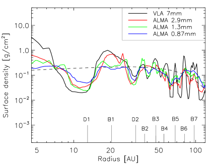
Figure 2: Surface density profiles obtained from fitting the brightness distributions along the disk major axis at each wavelength (see Sect. 3). The dashed line represents a tapered-edge model: $\Sigma(R)\propto(R/R_{\rm C})^{-\gamma}\,{\rm exp}[-(R/R_{\rm C})^{2-\gamma}]$ with $R_{\rm{C}}=78.9\,\rm{AU}$ and $\gamma=-0.22$ from Kwon et al. (2011). Selected gaps and rings identified by ALMA Partnership et al. (2015) are indicated. $\Sigma_{\rm VLA}$ ($7\,\rm{mm}$) is shown as black, $\Sigma_{\rm B3}$ ($2.9\,\rm{mm}$) as red, $\Sigma_{\rm B6}$ ($1.3\,\rm{mm}$) as green, and $\Sigma_{\rm B7}$ ($0.87\,\rm{mm}$) as blue lines.

2.2 Grain properties

We assume that the dust grains are a mixture of 75% amorphous silicate and 25% carbon, with a mean density of $\rho_{\rm{grain}}=2.5\,{\rm g\,cm^{-3}}$. The complex refractive indices are given by Dorschner et al. (1995) and Jäger et al. (1998). The grain size distribution follows the standard power law ${\rm d}n(a)\propto{a^{p}}{\rm d}a$ with a minimum grain size of $a_{\rm{min}}=0.01\,\mu{\rm m}$. We fix the maximum grain size to $a_{\rm{max}}=7\,\rm{mm}$, which is identical to the longest wavelength of the used data sets. The observations at 7 mm are not sensitive to larger grains. We consider 25 size bins that are logarithmically spaced between the minimum and maximum grain sizes. The dust extinction coefficients are computed using Mie theory. Initially, we use $p=-3.5$ (constant over the whole disk). However, the parameter $p$ eventually has to be modified locally due to the effects of dust evolution. Therefore, as our modeling progresses, we deviate from the assumption of radially constant values for $p$ over the whole disk (see Sect. 5.2). Figure 1 provides an illustration of the average absorption and scattering opacities over the whole grain size distribution with $p=-3.5$.

2.3 Stellar heating

The disk is assumed to be passively heated by stellar irradiation (e.g., Chiang & Goldreich, 1997). We take the Kurucz atmosphere models with ${\rm log}\,g=3.5$ as the incident stellar spectrum (Kurucz, 1994). The radiative transfer problem is solved self-consistently considering 150 wavelengths, which are logarithmically distributed in the range of [$0.1\,\mu{\rm{m}}$, $10000\,\mu{\rm{m}}$]. The effective temperature of the star was fixed to $4000\,\rm{K}$. For the stellar luminosity, we first adopted a value of $L\sim 6\,L_{\odot}$ as derived by White & Hillenbrand (2004) from an analysis of HL Tau’s optical spectrum. However, we found that models with this luminosity significantly underestimate the fluxes at all ALMA and VLA bands, even with an unreasonably large disk mass. Therefore, we increased the stellar luminosity to $11\,L_{\odot}$, which is identical to the value used in Men’shchikov et al. (1999) and Pinte et al. (2016). In White & Hillenbrand (2004), the effective temperature of the star was taken to be 4395 K, whereas we adopted a value of 4000 K. The difference in this quantity can result in different luminosities.

The disk can be actively heated by the loss of gravitational energy released from material as it accretes through the disk onto the central star (e.g., D’Alessio et al., 1998), which is known as viscous heating. This heating mechanism might be important in early evolutionary stages (e.g., Class 0/I object), since the accretion rate is much higher than for more evolved sources. We estimated the accretion luminosity using the approximate formula:

$$L_{\rm{acc}}=\frac{G\dot{M}_{{\rm acc}}M_{\star}\left(1-\frac{R_{\star}}{R_{{\rm in}}}\right)}{R_{\star}}$$ (4)

where $R_{\rm{in}}$ denotes the truncation radius of the inner disk and is set to be $5\,R_{\star}$ (Gullbring et al., 1998). The gravitational constant is $G$. The stellar radius ($R_{\star}$) is taken to be $7\,R_{\odot}$ and mass ($M_{\star}$) is $1.7\,M_{\odot}$ (Pinte et al., 2016). With the accretion rate $\dot{M}_{\rm{acc}}=1.6\times 10^{-7}\,M_{\odot}/yr$ measured by White & Hillenbrand (2004), we derived an accretion luminosity of $0.98\,L_{\odot}$ that is about $10\%$ of the assumed stellar luminosity. Furthermore, accretion disk theory shows that only about ${<}\,50\%$ of this accretion energy contributes to the heating of circumstellar disks (e.g., Calvet & Gullbring, 1998). Therefore, we neglected viscous heating in our simulation.

Table 1: Model parameters.

Parameter	Model A	Model B	Model C
Stellar parameters
$M_{\star}\,[M_{\odot}]$	1.7
$T_{\star}\,[\rm K]$	4000
$L_{\star}\,[L_{\odot}]$	11
Disk parameters
$\beta$	1.15	$1.14^{+0.018}_{-0.007}$	$1.08^{+0.03}_{-0.005}$
$H_{100}(a_{\rm min})\,{\rm[AU]}$	15	$13.7^{+1.6}_{-1.0}$	$10.6^{+4.3}_{-1.1}$
$M_{\rm dust}\,[10^{-3}\,M_{\odot}]$	1.0	$1.0^{+0.12}_{-0.1}$	$1.0^{+0.07}_{-0.16}$
$p$	$-3.5$	–	–
$p_{\rm inner}$	–	$-3.45^{+0.08}_{-0.17}$	–
$p_{\rm outer}$	–	$-3.92^{+0.18}_{-0.08}$	–
$f_{\rm inner}$	–	$0.5^{+0.03}_{-0.11}$	–
$f_{2.82}$	–	–	$0.27^{+0.05}_{-0.07}$
$f_{0.95}$	–	–	$0.15^{+0.07}_{-0.03}$
$f_{0.45}$	–	–	$0.20^{+0.03}_{-0.06}$
$f_{0.29}$	–	–	$0.15^{+0.05}_{-0.05}$
Observational parameters
$i\,[^{\circ}]$	46.7
Position angle [∘]	138
$D\,{\rm[pc]}$	140

3 Building the surface density profile

The surface density $\Sigma(R)$ is needed to complete the setup of a disk model (see Eq. 1). It is commonly approximated by a simple analytic expression, in most previous studies by a power-law profile. However, ALMA observations at all three bands show a set of bright and dark rings in the HL Tau disk, while the VLA image unveils the structure of the first ring at a comparable spatial resolution. It is also obvious from these images that the gap depths (i.e., depletion factor of dust in the dark rings) are different between rings. Consequently, it is not practical to describe the surface density with a parameterized formula. Instead, we build the surface density of the model by reproducing the brightness distribution at each wavelength along the disk major axis.

We used the method introduced by Pinte et al. (2016) to construct the surface density profile with an iterative procedure. We extracted the observed brightness profiles along the major axis of the disk in the CLEANed maps and took an average of both sides. We started with a simple power-law surface density with an exponent of $-0.5$. The choice of this starting profile does not really matter, since it is only used for the first iteration. Using the radiative transfer code RADMC-3D, we produced synthetic images at each wavelength and convolved them with appropriate Gaussian beams. When doing this, we actually simulated two images with different field of views: $30\,\rm{AU}$ and $300\,\rm{AU}$. Both images feature an identical number of pixels. Therefore, the image with the smaller field of view has a ten times better resolution than that of the other one. We combined both images into a new one after rebinning them to the pixel scale of the image with the smaller field of view. The extraction of model brightness distributions is performed on the new image. This procedure is employed to ensure that the radiative transfer models sufficiently resolve the inner disk, which is required to reproduce the central emission peak seen in both the ALMA and VLA images. In subsequent iterations, the surface density at each radius ($R$) is corrected by the ratio of the observed and the modeled brightness profile. The iteration procedure continues until the change in the model brightness profile is smaller than 2% at any radius. It took about 35 iterations to reach convergence and was individually performed for each of the maps.

In order to keep the procedure as simple as possible, we initially fixed $H_{100}(a_{\rm min})\,{=}\,15\,\rm{AU}$ and $\beta\,{=}\,1.15$, which are typically found for other disks (e.g., Andrews et al., 2009; Madlener et al., 2012; Liu et al., 2012; Kirchschlager et al., 2016). The disk inclination ($i\,{=}\,46.7^{\circ}$) and position angle (${\rm PA}\,{=}\,138^{\circ}$) are adopted from the ALMA Partnership et al. (2015). The slope of the grain size distribution is constant throughout the disk with $p\,{=}\,-3.5$. Table 3 gives an overview of the model parameters and model A corresponds to the setup assumed here. Figure 2 shows the result. The four surface density profiles are similar in general and we can broadly identify similar gap locations from them. For convenience of the subsequent parameter study, we use $\Sigma_{\rm{VLA}}$, $\Sigma_{\rm{B3}}$, $\Sigma_{\rm{B6}}$, and $\Sigma_{\rm{B7}}$ to label the surface density profiles that individually match the observed brightness distributions along the major axis of the disk at the wavelengths of 7 mm, 2.9 mm, 1.3 mm, and 0.87 mm, respectively.

4 Modeling steps and fitting approach

We have obtained four individual surface density profiles so far from reproducing the VLA and three ALMA images separately. The next step is to use one (or a combination) of them to search for a coherent model that can explain the four images simultaneously. In this section, we introduce the steps towards this goal and describe the approach to conduct the fitting task and the error estimate for the best-fit model.

4.1 Modeling steps

In any modeling approach, it is preferable to build a model with as few free parameters as possible. Therefore, our modeling consists of three steps, from a simple scheme gradually to a more complex setup as required by the data. First, we directly take each of the four surface density profiles to check whether a radially homogeneous grain size distribution is sufficient to explain all the data (see Sect. 5.1). Secondly, we treat the inner (${<}\,50\,\rm{AU}$) and outer (${>}\,50\,\rm{AU}$) disks separately by assuming different grain size distributions. We conduct a large parameter study and figure out if this new setup can reproduce all the observations (see Sect. 5.2). Lastly, we particularly parameterize the mass fractions of large grains with certain grain sizes and present a coherent model of HL Tau (see Sect. 5.3).

4.2 Fitting approach

4.2.1 Staggered Markov chains

We run three families of models, each of which has different degrees of freedom. The fitting task was performed with a simulated annealing (SA) algorithm (Kirkpatrick et al., 1983), which has already been demonstrated to be successful for disk modeling (Madlener et al., 2012; Liu et al., 2012). Based on the Metropolis-Hastings algorithm, SA creates a Markov Chain Monte Carlo (MCMC), random walk through the parameter space, thereby gradually minimizing the discrepancy between observation and prediction by following the local topology of the merit function, for example the $\chi^{2}$-distribution in our case. This approach has specific advantages for high-dimensionality optimization because no gradients need to be calculated and entrapment in local minima can be avoided regardless of the dimensionality.

Our aim is to fit all the brightness distributions in the three ALMA bands and at the VLA $7\,\rm{mm}$ band simultaneously. The traditional method used in multi-observable optimization is to minimize the combination of individual $\chi_{k}^{2}$ values from fitting each image

$$\chi^{2}_{\rm total}=\sum_{k=1}^{N}g_{k}\,\chi^{2}_{k},$$ (5)

which introduces arbitrary weightings ($g_{k}$) for each dataset. However, it is difficult to choose the coefficients $g_{k}$, because the signal-to-noise ratio (S/N) can differ between observables. In order to circumvent this problem, we devised a staggered Markov chain (for details see Madlener et al., 2012). The general idea is to keep track of individual annealing temperatures of the Markov chains for every dataset and perform a Metropolis-Hastings decision for accepting a proposed model or rejecting it after each individual calculation of $\chi^{2}_{k}$. The 7, 2.9, 1.3, and 0.87 mm images are fitted in a sequential order. The synthetic image at one particular wavelength is produced when the proposed model is accepted in the fitting of images at all longer wavelengths. By only accepting new configurations after all individual $\chi^{2}_{k}$ steps were completed successfully, the algorithm effectively optimizes all observational data sets simultaneously without the need for weighting them.

4.2.2 Criteria for chain termination

Since it is difficult to give an upper bound for the number of steps to reach the global optimum, we need to define a reasonable criterion to stop an optimization run. We randomly selected the starting points, propagated the chains, and monitored the quality of the fit. We found that a typical number of ${\sim}1000$ steps is required to achieve a “good” solution regardless of the starting points. This number has also been suggested by previous multi-wavelength modeling of circumstellar disks (Madlener et al., 2012). We refrained from using a strict $\chi^{2}$ criterion to identify “good” solutions since we are interested here in capturing especially the qualitatively fine structure of the radial profiles (gaps and rings), and a model with a low $\chi^{2}$ does not always reproduce these features correctly. Therefore, for each family of models, we calculated 15 different MCMCs starting from randomly chosen models and we let them run for 1000 steps to search for the best solution.

4.2.3 Error estimation

Estimation of the uncertainties for the best-fit model using SA is not as straightforward as in other methods like Bayesian analysis. First, a confidence interval $\chi^{2}_{\rm conf}$ has to be defined from already calculated models. Secondly, the vicinity of the best-fit in parameter space is probed by starting one Markov chain from this location. After collecting sufficient parameter sets below the confidence threshold, this normally asymmetric domain can be characterized by taking the minimum and maximum values of each degree of freedom.

We calculated a new Markov chain from the best-fit model to sample the $\chi^{2}$-distribution. A low chain temperature and small step widths for each parameter are adopted to restrain the random walk to the vicinity for sufficient steps. The total acceptance ratio of the models in this chain is ${\sim}\,0.2$. We gathered ∼100 accepted samples below the confidence threshold $\chi^{2}_{\rm conf}$ defined by

$$\chi^{2}_{\rm conf}<1.5\cdot\chi^{2}_{\rm min},$$ (6)

where $\chi^{2}_{\rm min}$ is the new overall minimum $\chi^{2}$ if found during the restarted run. In order to define $\chi^{2}_{\rm min}$ here, we have to use Eq. 5 to get a compromise between the quality of the fits to each map. The coefficients $g_{k}$ are chosen in a way that the contributions to the $\chi^{2}$ come into balance between different maps. We should stress that our criterion for defining the confidence region is not universal due to the non-linearity of the high-dimensional models and the difference in the $\chi^{2}-$distribution between optimization problems.

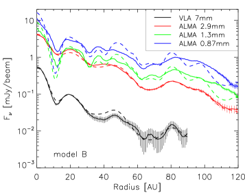
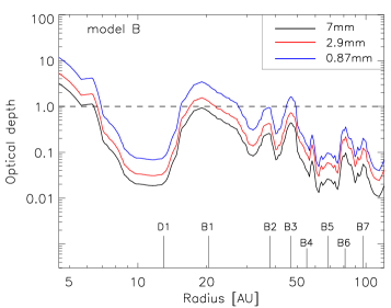
Figure 3: Top panel: Observed (solid lines) and synthetic (dashed lines) flux distributions along the major axis of the disk. The results are for model B, in which the inner ($<50\,\rm{AU}$) and outer ($>50\,\rm{AU}$) disks have different grain size distributions (see Sect. 5.2). For better representation, we only show the error bars of the observations which are larger than 5% of the fluxes. VLA $7\,\rm{mm}$ data are shown as black, band 3 as red, band 6 as green, and band 7 as blue lines. The VLA data at $R\,{>}\,{\sim}\,90\,\rm{AU}$ are not shown because of a low signal-to-noise ratio. Middle panel: The combined surface density profile of model B. Bottom panel: the vertical optical depth of as a function of radius at 7, 2.9, and $0.87\,\rm{mm}$ wavelength.

5 Results

5.1 Modeling with a homogeneous grain size distribution

Taking each of the four surface density profiles (i.e., $\Sigma_{\rm{VLA}}$, $\Sigma_{\rm{B3}}$, $\Sigma_{\rm{B6}}$, or $\Sigma_{\rm{B7}}$) as the input individually, we explored the parameter space defined as {$\beta$, $H_{100}$, $M_{\rm dust}$, $p$}. In other words, these parameters are allowed to vary freely. However, we could not find a model that reproduces all the observations simultaneously. This is an indication that the grain size distribution is radially changing. First hints for a radial drift of larger grains toward the inner disk have already been found by Pinte et al. (2016) and Carrasco-González et al. (2016).

5.2 Modeling with two power-law grain size distributions

From a modeling analysis of HL Tau, Pinte et al. (2016) found that the grain size distribution has a local slope close to $-3.5$ up to $75\,\rm{AU}$, while the outer disk features a steeper slope of $-4.5$, indicating that large grains in the outer disk are depleted. For optically thin emission in the Rayleigh-Jeans regime, the spectral index is a probe for the particle size (Beckwith et al., 2000). Carrasco-González et al. (2016) calculated the spectral index $\alpha_{7-2.9\,\rm mm}$ between $7$ and $2.9\,\rm{mm}$ for the HL Tau disk. Their results show a clear gradient in $\alpha_{7-2.9\,\rm mm}$ between ${\sim}10$ and $50\,\rm{AU}$, with a lower value closer to the central star. The fact that larger grains are located at smaller radii is in agreement with general trends in theoretical predictions (Birnstiel et al., 2010b; Ricci et al., 2010a, b; Testi et al., 2014) and with observational constraints on several disks (e.g., Pérez et al., 2012, 2015).

We therefore modify our model by introducing two new parameters, $p_{\rm inner}$ and $p_{\rm outer}$, to describe the grain size slope for the inner and outer disk, respectively. The two slopes are adjustable to control the contributions from large grains. Changing the maximum grain size $a_{\rm max}$ basically has the same effect. Therefore, we fixed $a_{\rm max}\,{=}\,7\,\rm{mm}$ in both the inner and outer disk to reduce the model degeneracy.

Among the observations considered here, 7 mm and 2.9 mm are the two longest wavelengths. The VLA observation at 7 mm is sensitive to the inner disk, while the structure of the outer disk is revealed by the ALMA observation. Therefore, for the inner 50 AU, we take $\Sigma_{\rm{VLA}}$ as the surface density. For the outer 50 AU, we use $\Sigma_{\rm{B3}}$. We chose $50\,\rm{AU}$ as the border for two reasons. First, Pinte et al. (2016) show that disk regions inside this radius are (marginally) optically thick at the ALMA wavelengths. Therefore, the ring properties inside $50\,\rm{AU}$, derived by exclusively using the ALMA data, are poorly constrained. Secondly, the signal-to-noise ratio of the VLA data outside $50\,\rm{AU}$ is obviously lower compared to the inner parts.

We introduce $f_{\rm inner}$ as a control parameter on the total dust mass of the inner ($R\,{<}\,50\,\rm{AU}$) disk. The mass fraction of the outer disk is derived via $1-f_{\rm inner}$. The parameter space is now {$\beta$, $H_{100}$, $M_{\rm dust}$, $p_{\rm inner}$, $p_{\rm outer}$, $f_{\rm inner}$} (see model B in Table 3). We conduct a large parameter study with the MCMC method. Figure 3 (top panel) shows the fitting result, while the combined surface density profile of the best model is displayed in the middle panel. We can see that the predicted flux distributions are in good agreement with the observations at both 7 and 2.9 mm. The model successfully reproduces the main features (e.g., the location and width for most dark rings) of the 1.3 and 0.87 mm images as well. However, the model brightness profiles at these two wavelengths appear to have bumps and wiggles. In particular, the depth of the D1 ring ($R\,{\sim}\,13\,\rm{AU}$) at 1.3 mm (band 6) and 0.87 mm (band 7) is deeper than that of the observations. This is mainly due to the fact that the model does not make use of the surface density profiles $\Sigma_{\rm B6}$ and $\Sigma_{\rm B7}$, and the real grain size distribution in the HL Tau disk is certainly more complex than the assumed prescription. In comparison to the best-fit grain size slope of the inner disk $p_{\rm inner}=-3.5^{+0.1}_{-0.2}$, we observe a steeper grain size slope $p_{\rm outer}=-3.9^{+0.2}_{-0.1}$ in the outer disk, indicating that large grains are more concentrated in the inner region of the HL Tau disk. Figure 3 (bottom panel) displays the vertical optical depth as a function of radius, from which we demonstrate that the thermal dust emission from the inner (B1 and B3) rings are optically thick at the ALMA wavelengths, while most parts (i.e., ${>}\,6\,\rm{AU}$) of the disk becomes optically thin at the VLA 7 mm.

Table 2: Ring properties.

Ring	Radius range	Dust Mass ($M_{\oplus}$)2
	[AU]	Our work	Carrasco-Gonzalez et al. (2016)	Pinte et al. (2016)
Peak	$<13$	$16^{+2}_{-4}$	10$-$50	$>2.3$
B1	13$-$32	$43^{+2}_{-7}$	70$-$210	$>47$
B2	32$-$42	$24^{+1}_{-4}$	30$-$90	30$-$69
B3	42$-$50	$30^{+2}_{-5}$	20$-$80	14$-$37
B4	50$-$64	$35^{+2}_{-6}$	30$-$90	40$-$82
B5	64$-$74	$17^{+2}_{-3}$	10$-$50	5.5$-$8.7
B6	74$-$90	$65^{+3}_{-9}$	40$-$140	84$-$129
B7	90$-$150	$118^{+5}_{-20}$	–	99$-$157

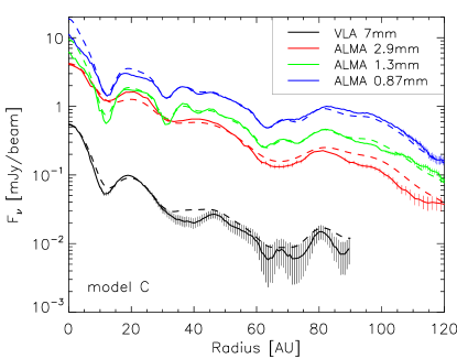
Figure 4: Same as in the upper panel of Figure 3, but for model C (see Sect. 5.3).

5.3 Modeling with complex grain size distributions

By assuming different grain size slopes for the inner and outer disks, model B can explain the 7 and 2.9 mm data well. However, the quality of the fit to the 1.3 and 0.87 mm images is not very satisfying. In order to build a single model that reproduces the four bands simultaneously, we adopt a procedure similar to the one used in Pinte et al. (2007, 2016). We utilize the four derived surface density profiles and assign each of them to a single grain size, which emits most at a particular wavelength. The surface densities $\Sigma_{\rm VLA}$, $\Sigma_{\rm B3}$, $\Sigma_{\rm B6}$, and $\Sigma_{\rm B7}$ were used to define the density distribution of the grains of size 2.82, 0.95, 0.45, and 0.29 mm respectively. For all the grains with sizes in the range of [$0.01\,\mu{\rm{m}}$, 0.29 mm], their surface densities are incorporated into $\Sigma_{\rm B7}$, independently of their size. Similarly, we use $\Sigma_{\rm VLA}$ to distribute all the remaining grains larger than 2.82 mm. Although dust of a single given grain size does not emit only at the corresponding wavelength, the contamination between bands is negligible because the emissivity as a function of the wavelength of a given grain size has a clear peak at these wavelengths.

We introduce four parameters $f_{2.82}$, $f_{0.95}$, $f_{0.45}$, and $f_{0.29}$. These are mass ratios. For each of the four special grain sizes mentioned above, these ratio parameters denote the mass of all grains put into such a specific size (2.82, 0.95, 0.45, and 0.29 mm, respectively) divided by the entire dust mass $M_{\rm dust}$ of all grains considered (spanning a range of sizes from 0.01 $\mu$m up to 7 mm). Therefore, the combined mass of grains that are either smaller than $0.29\,\rm{mm}$ or larger than $2.82\,\rm{mm}$ is thus a dependent variable through the expression $[(1-(f_{2.82}+f_{0.95}+f_{0.45}+f_{0.29})]\times M_{\rm dust}$. As a result, the size distribution at any radius is no longer a simple power law. This new setup has a parameter space of {$\beta$, $H_{100}$, $M_{\rm dust}$, $f_{2.82}$, $f_{0.95}$, $f_{0.45}$, $f_{0.29}$}. Figure 4 shows the best result from the MCMC optimization, whereas a summary of the model parameters (i.e., model C) can be found in Table 3. The resulting model brightness distributions are now in excellent agreement with the observed ones at all four wavelengths.

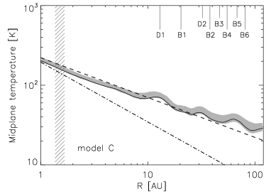
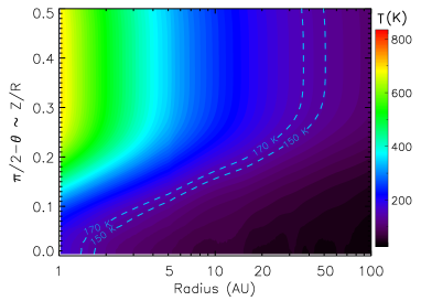
Figure 5: Left panel: Temperature distribution in the disk midplane. The black solid line refers to model C, whereas the shaded region shows the results of all models within the confidence interval. The dashed line represents a power-law distribution: $T_{\rm dust}=T_{0}(R/R_{0})^{-q}$ with $q=0.5$, $T_{0}=70\,\rm{K}$ and $R_{0}=10\,\rm{AU}$, which is one of the assumed temperature distributions from Carrasco-González et al. (2016). The dash-dotted line shows the effective temperature distribution of the disk if disk accretion is the only heating source (see Sect. 6.1). The hashed region corresponds to the location of water snow-line ($R\,{\sim}\,1.5\,\rm{AU}$) assuming an ice sublimation temperature of $150{-}170\,\rm{K}$. Right panel: The temperature structure as a function of radius $R$ and polar angle $\theta$ in spherical coordinates ($\pi/2$ is the equatorial plane, i.e., the bottom of the figure) for model C. The 150 K and 170 K contours are indicated with dashed lines.

We show the temperature distribution in the disk midplane in the left panel of Figure 5. The profile generally follows a power law. The temperature increases at ${\sim}\,10\,\rm{AU}$ and ${\sim}\,30\,\rm{AU}$ are presumably dominated by the indirect irradiation of the thermal emission from the B1 and B2 rings, while the other bump at ${\sim}\,60\,\rm{AU}$ can be explained by the density enhancement of dust grains within the B5 ring. We manually removed the B1 and B2 rings in the simulation to test this speculation. The results show that the bumps in the midplane temperature distribution disappear when there is no bright irradiation source adjacent to the bump location. These fluctuations are also not caused by the noise of Monte-Carlo radiative transfer because models with many more photon packages show the same behavior. The right panel of Figure 5 shows the two-dimensional temperature structure of the disk. Snow-lines of volatile species play an important role in planet formation theories (e.g., Pontoppidan et al., 2014). Assuming an ice sublimation temperature of $150{-}170\,\rm{K}$ (e.g., Podolak & Zucker, 2004), the water snow-line is located at a radius range from ${\sim}\,1.5\,\rm{AU}$ in the midplane up to ${\sim}\,40\,\rm{AU}$ in the surface layers of the disk.

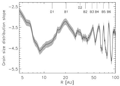
Figure 6: Slope of the local grain size distribution as a function of radius. The black solid line refers to model C, whereas the shaded region shows the results of all models within the confidence interval (see Sect. 5.3).

From the best fit, we calculate the ring properties that are summarized in Table 4. The nomenclature of the rings is the same as in ALMA Partnership et al. (2015). The ring masses are calculated by integrating the surface density over the radius range between two successive gaps. In order to have a direct comparison with the literature results, these radius ranges are identical to those used in Pinte et al. (2016) and Carrasco-González et al. (2016), which we list in Table 4.

We convert the masses of grains with sizes of 2.82, 0.95, 0.45, and 0.29 mm to the particle numbers $n(a)$ and vertically integrate them within a column ($R$). We perform a linear fit to the relation ${\rm log}\,n(a)\,vs.\,{\rm log}\,a$ to obtain the local grain size slope. The result is shown in Figure 6. Although we see a general radial change in grain size from dominant smaller grains ($p\,{=}\,-4.5$) to larger grains ($p\,{=}\,-3.5$) in the inner disk, we obtain, for the first time, a spatially resolved size distribution. We clearly see that larger grains are accumulated in the surface density peaks, especially in the B1 ring ($R\,{\sim}\,20\,\rm{AU}$), where the grain size distribution has a local slope close to $p=-3.2$ (see Figure 6).

6 Discussion

In this section, we discuss our results concentrating on the following aspects: the properties of the inner disk, the disk instability, and the size distribution of dust particles.

6.1 The properties of the inner disk

As laid out in Sect. 5.3, we derived the masses of various rings and showed the temperature profile of the disk. According to the definition of the ALMA Partnership et al. (2015), the gap$-$ and ring$-$like structure of the HL Tau disk is located at a radius range from ${\sim}13$ to ${\sim}90\,\rm{AU}$, that is, from the D1 to D7 dark rings. As shown in the bottom panel of Figure 3, the 7 mm dust thermal emission is optically thin beyond ${\sim}\,6\,\rm{AU}$, which indicates that the specific inclusion of the VLA data into the self-consistent modeling places stringent constraints on the properties of the disk, especially in the inner region, in contrast to the optically thick ALMA data.

The temperature profile in the disk midplane generally follows a power law, decreasing from ${\sim}\,90\,\rm{K}$ at 5 AU to ${\sim}\,25\,\rm{K}$ at 100 AU. Jin et al. (2016) presented a representative radiative transfer model of the HL Tau disk. In order to investigate whether the observed ring and gap features can be produced by planet-disk interaction, the density structure of their model is obtained from two-dimensional hydrodynamic simulations with the inclusion of three embedded planets and disk self-gravity. Their model features a lower midplane temperature of ${\sim}20\,\rm{K}$ at 100 AU and a somewhat higher temperature of ${\sim}110\,\rm{K}$ at 5 AU. The discrepancy between our and their results is mainly due to the fact that we assumed different minimum and maximum grain sizes and dust composition. Pinte et al. (2016) obtained a similar temperature of ${\sim}20\,\rm{K}$ at 100 AU. Carrasco-González et al. (2016) analytically estimated the total dust mass of the HL Tau disk by assuming a power-law temperature profile $T_{\rm dust}=T_{0}(R/R_{0})^{-q}$. In order to take the uncertainties of temperature into account, they explored a wide range of $q$ and $T_{0}$ in their analysis. The dashed line in Figure 5 (left panel) illustrates the result with $q=0.5$ and $T_{0}=70\,\rm{K}$ at $R_{0}=10\,\rm{AU}$, close to the lower limit of temperatures they considered. The temperature distribution from our self-consistent modeling is in agreement with the temperature profile assumed by Carrasco-González et al. (2016), but in addition our results are susceptible to localized temperature changes in the rings. We also calculated the effective temperature of the disk when only viscous heating is considered as the heating process using the formula:

$$T_{\rm eff,disk}=\left(\frac{3}{8\pi\sigma_{\rm{SB}}}\dot{M}_{\rm{acc}}\Omega^{2}_{K}(R)\right)^{1/4},$$ (7)

where $\sigma_{\rm{SB}}$ refers to the Stefan-Boltzmann constant and $\Omega_{K}(R)$ is the angular frequency (Knigge, 1999). The result is shown as a dash-dotted line in Figure 5 (left panel). It can be seen that the effective temperatures at each radii are much lower than the midplane temperatures, which demonstrates again that an inclusion of viscous heating into the modeling does not significantly change the temperature structure of HL Tau’s disk.

The ring masses range from $16$ to $120\,M_{\oplus}$. Our results are generally consistent with the values given by Pinte et al. (2016) and Carrasco-González et al. (2016). However, for individual rings there is some discrepancy probably due to the different choice of dust properties and optical depth effect affecting previous studies. In particular, we deduce a lower (almost two times) mass for B2 and B6 rings compared to the values presented in Pinte et al. (2016). In order to match the central peak emission in the ALMA images, Pinte et al. (2016) fixed the surface density in the central 5 AU to a power-law profile with a slope of $-0.5$ and manually added some unresolved emission at the position of the star in the simulated maps. Their results show that the dust emission from B2, B3, and B6 rings is marginally optically thick at 2.9 mm, according to the criterion of $1<\tau_{2.9\,\rm{mm}}<3$. In our approach, we produce two images with fields of view of 30 and 300 AU at one particular wavelength. The simulated image focused on the central region has a better resolution and can help to get close to the correct flux prediction. By conducting a large parameter study, the optimization algorithm tends to put more dust near the center to reproduce the peaks, but without any further addition of emission. This is the reason why a clear increase appears in the surface density profile towards the central star (see the black line in Figure 2). As a consequence, the outer region where these rings are located shares less of the disk’s mass. From the bottom panel of Figure 3, one can see that the dust thermal emission from the B2, B3, and B6 rings is optically thin at both 2.9 and 7 mm. Hence, the inclusion of the VLA observation into the modeling analysis clearly improves the constraint on the ring properties. With the dust properties described in Sect. 2.2, model C has an average (averaged over the whole radius range) dust mass extinction coefficient at 7 mm of $\kappa_{\rm{abs}}{+}\kappa_{\rm{sca}}=1.6\,\rm{cm^{2}/g}$, which is clearly larger than the maximum value of $0.2\,\rm{cm^{2}/g}$ considered in Carrasco-González et al. (2016). As a result, we obtained systematically lower ring masses than their results.

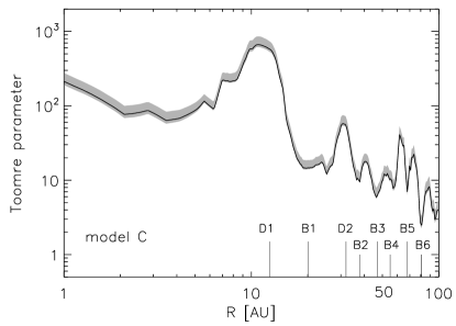
Figure 7: Toomre parameter as a function of radius. The black solid line refers to model C, whereas the shaded region shows the results from all the models within the confidence interval.

6.2 Disk instability

The highest angular resolution VLA images of the HL Tau disk reveal a compact knot structure in the first bright ring (B1) (Carrasco-González et al., 2016). This knot also coincides with a local intensity maximum in the ALMA 1.3 mm image. One of the formation mechanisms of a clumpy structure is gravitational instability (GI) of massive disks.

We checked this possibility using the Toomre criterion (Toomre 1964) that describes when a disk becomes unstable through gravitational collapse. The Toomre $Q$ parameter is defined as

$$Q=\frac{c_{s}\Omega_{k}}{\pi G\Sigma},$$ (8)

where $c_{s}$ is the local sound speed and $\Sigma$ stands for the surface density of the gas. In terms of $Q$, a disk is unstable to its own self-gravity if $Q<1$, and stable if $Q>1$. Figure 7 displays the Toomre parameter as a function of radius. We assumed a constant dust-to-gas mass ratio of 0.01 throughout the disk for simplicity. However, Yen et al. (2016) analyzed the ${\rm HCO^{+}(1-0)}$ data of HL Tau obtained from ALMA. Their results indicate that the dust-to-gas mass ratio probably varies as a function of radius. In particular, they found a relatively higher fraction of gas in the first dark (D1) ring. Taking this fact into account, the prominent bump of $Q$ at the location of the D1 ring will be reduced (see Figure 7).

It is clear that the $Q$ value is greater than unity for the entire disk. However, for $R\,{>}\,80\,\rm{AU}$, the disk is close to the threshold of being gravitationally unstable. This is consistent with the recent finding by Akiyama et al. (2016) that the GI can operate most probably in the outer region of the HL Tau disk. Pohl et al. (2015) showed that an embedded massive planet (planet-to-star mass ratio of 0.01) can trigger a gravitational instability in massive disks with a Toomre parameter around unity. Assuming a stellar mass of $1.7\,M_{\odot}$, a planet with a mass of ${>}18\,M_{\rm{Jup}}$ is required. With direct mid-IR imaging, Testi et al. (2015) set an upper limit of ${\sim}10{-}15\,M_{\rm{Jup}}$ (i.e., smaller than the required mass) for planetary objects present in the D5 and D6 dark rings. However, massive planets may exist in other locations, and the effect of multiple (small mass) planets on the reduction of the Toomre parameter has not yet been investigated.

Another possibility for a driver of structure formation, however, is secular GI. Secular GI is the gravitational collapse of dust due to gas$-$dust friction (e.g., Ward, 2000; Youdin, 2011). Recently, secular GI has been proposed as an underlying mechanism for multiple ring$-$like structures (Takahashi & Inutsuka, 2014). Using physical parameters derived from the ALMA observations, Takahashi & Inutsuka (2016) performed a linear stability analysis of secular GI, and verified that it can cause the ring structures observed in HL Tau under certain conditions. The assumed temperature distribution, surface density, and maximum grain size (as the main inputs of the secular GI analysis) agree well with what we obtained from modeling the VLA and ALMA observations simultaneously. Since secular GI can concentrate the dust and support dust growth, the observed dust clump may be a consequence of dust condensation in the first bright ring (B1) induced by secular GI.

6.3 Grain size distribution

The growth of dust grains from sub$-$$\mu\rm{m}$ to millimeter sizes is the first step towards the formation of planetesimals (e.g., Papaloizou & Terquem, 2006; Lissauer & Stevenson, 2007; Natta et al., 2007). Brauer et al. (2008) and Birnstiel et al. (2010a) have modeled the evolution of dust grain populations with a sophisticated treatment of the dust growth processes and the dynamical mechanisms responsible for the transport of dust grains in disks. These theoretical studies predict that dust properties change as a function of the radius, with more large dust grains located at smaller radii (see also Birnstiel et al., 2010b).

The (sub-)millimeter spectral slope ($\alpha$) derived from spatially resolved observations is a common probe for grain size: low values of $\alpha$ can be interpreted in terms of grain growth (e.g., Isella et al., 2010; Guilloteau et al., 2011). Radius-dependent dust properties have been observed for a number of disks, for example AS 209 (Pérez et al., 2012), CY Tau, and DoAr 25 (Pérez et al., 2015). Moreover, Trotta et al. (2013) and Tazzari et al. (2016) carried out self-consistent modeling works of the disk structure and the dust properties by fitting interferometric observations of a sample of targets using a radius-dependent grain size distribution. Their results confirm the radial variation of grain growth, with the maximum grain size decreasing with radius.

Carrasco-González et al. (2016) calculated the spectral index $\alpha_{7-2.9\,\rm{mm}}$ between 7 and 2.9 mm, which are currently the two most optically thin wavelengths of the observations for HL Tau. The authors witnessed a clear radial gradient in $\alpha_{7-2.9\,\rm{mm}}$ that is consistent with a change in dust properties and a differential grain size distribution, with more larger grains at smaller radii. This is confirmed by our modeling. Model B presented in Sect. 5.2 has a grain size slope of $p_{\rm inner}=-3.5^{+0.1}_{-0.2}$ in the inner disk and a steeper value of $p_{\rm outer}=-3.9^{+0.2}_{-0.1}$ for the outer ($R\,{>}\,50\,\rm{AU}$) disk. Pinte et al. (2016) also obtained a shallower slope at smaller radii from modeling the ALMA data. Model C shows the same general trend, with $p$ approaching values of $-4.5$ beyond 60 AU (see Sect. 5.3). In addition, model C reveals that the slope for the grain size distribution has local maxima associated with many of the bright rings. For instance, the grain size distribution of the B1 ring ($R\,{\sim}\,20\,\rm{AU}$) has a local slope close to $p=-3.2$ This can be interpreted as an indication for a concentration of larger grains in such regions. All this suggests that dust growth and concentration of large grains, as initial steps of planet formation, have already occurred in HL Tau at the relatively young age of ${\sim}1\,\rm{Myr}$.

7 Summary

We performed detailed radiative transfer modeling of the HL Tau disk. Both the ALMA images at 0.87, 1.3, and 2.9 mm and the recent VLA 7 mm map are taken into account. We first built the surface density profiles by inverting the observed brightness distributions along the major axis of the disk at each individual wavelength. Then, a large parameter study was conducted to search for a single model that can interpret all observations simultaneously. In order to reduce the model degeneracy as far as possible, our modeling starts from a simple assumption with a radially homogeneous grain size distribution, moving to a more complex scenario where the inner and outer disks feature different grain size slopes, to a prescription where the mass fractions of large dust grains are parameterized. We are able to place better constraints on the inner disk structure and the properties of different rings than all results exclusively based on ALMA observations because we added the more optically thin VLA 7 mm data to our analysis.

The temperature distribution in the disk midplane generally follows a power law, decreasing from ${\sim}\,90\,\rm{K}$ at 5 AU to ${\sim}\,25\,\rm{K}$ at 100 AU. The dust masses in the rings range from $16$ to $120\,M_{\oplus}$. We found a shallower slope of grain sizes in the inner disk, which indicates that a higher fraction of larger grains is present closer to the star. This is consistent with theoretical predictions of circumstellar disk evolution. In particular, many of the bright rings are associated with local maxima of the grain size distribution slope, indicating a concentration of larger grains in those rings. The Toomre parameter $Q$ is greater than unity for the entire disk. However, for $R\,{>}\,80\,\rm{AU}$, the disk is close to the threshold of being gravitationally unstable. We also discussed the origins of the dust clump in the first bright ring revealed by the VLA and suggested that secular GI is a promising mechanism.