Thermodynamics of metabolic energy conversion under muscle load

Abstract

The metabolic processes complexity is at the heart of energy conversion in living organisms and forms a huge obstacle to develop tractable thermodynamic metabolism models. By raising our analysis to a higher level of abstraction, we develop a compact — i.e. relying on a reduced set of parameters — thermodynamic model of metabolism, in order to analyze the chemical-to-mechanical energy conversion under muscle load, and give a thermodynamic ground to Hill’s seminal muscular operational response model. Living organisms are viewed as dynamical systems experiencing a feedback loop in the sense that they can be considered as thermodynamic systems subjected to mixed boundary conditions, coupling both potentials and fluxes. Starting from a rigorous derivation of generalized thermoelastic and transport coefficients, leading to the definition of a metabolic figure of merit, we establish the expression of the chemical-mechanical coupling, and specify the nature of the dissipative mechanism and the so called figure of merit. The particular nature of the boundary conditions of such a system reveals the presence of a feedback resistance, representing an active parameter, which is crucial for the proper interpretation of the muscle response under effort in the framework of Hill’s model. We also develop an exergy analysis of the so-called maximum power principle, here understood as a particular configuration of an out-of-equilibrium system, with no supplemental extremal principle involved.

1 Introduction

Thermodynamics provides the proper framework to describe and analyse the rich variety of existing sources of energy and the processes allowing its conversion from one form to another. Yet, of all known energy converters, man–made or not, living organisms still represent a formidable challenge in terms of thermodynamic modeling, due to their high complexity which far exceeds that of any other artificial or natural system [1, 2, 3, 4, 5, 6, 7, 8]. Energy conversion in living bodies is driven by metabolism, which ensures through chemical reactions at the cellular level, and along with other vital functions, the provision of heat necessary to maintain a normal body temperature, as well as, to a lesser extent, the energy required for muscular effort and motion. In the present work, we are particularly interested in catabolism, i.e. the energy-releasing process of breaking down complex molecules into simpler ones, and especially how, from a nonequilibrium thermodynamics viewpoint, the energy provided by the breaking of the digested food substances is made available to muscles for production of mechanical effort through contraction, as described in Hill’s model [9, 10]. The vision of Hill is summarized in the first statement of his Nobel Lecture in 1922:

“In investigating the mechanism involved in the activity of striated muscle two points must be borne in mind, firstly, that the mechanism, whatever it be, exists separately inside each individual fibre, and secondly, that this fibre is in principle an isothermal machine, i.e. working practically at a constant temperature.” [11]

Living organisms are open nonequilibrium and dissipative systems as they continuously exchange energy and matter with their environment [1, 2]. Unlike classical thermodynamic engines, for which equilibrium models may be built using extremal principles, no such a possibility exists for the case of living organisms because of the absence of identifiable genuine equilibrium states. Nevertheless, assuming a global system close to equilibrium, the development of a tractable thermodynamic model of metabolism may rely on notions pertaining to classical equilibrium thermodynamics: on the one hand, the working fluid acting as the conversion medium, and on the other hand, the characterization of its thermoelastic properties. Despite the complex features of biological systems, the identification of the nonequilibrium processes driving the transformation of the digested food chemical potential into a macroscopic form of energy made available for muscle work may be obtained from an effective locally linearized approach, ideally borrowing from the phenomenological approach to non-equilibrium thermodynamics developed by Onsager [12]. Application of Onsager’s approach and its integration on macroscopic systems make it possible to describe the behaviour of some thermodynamic conversion machines placed under mixed boundary conditions [13, 14, 15], which cause feedback effects and the emergence of complex dynamic behaviours [16]. We propose here to apply this approach to the case of living organisms viewed foremost as chemical conversion machines. In this article we thus derive first the macroscopic response from the local Onsager response. We then use the obtained results to compare the predictions of the model with the emblematic case of the muscle response proposed by Hill.

Before we proceed with the thermodynamics of metabolism, it is useful to first clarify what we mean by energy conversion in a standard thermodynamic engine. When energy is transferred to a system, its response manifests itself on the microscopic level through the excitation of its individual degrees of freedom and also on the global level whenever collective excitations are possible. In generic terms, a thermodynamic machine is the site of the conversion of a “dispersed” incident energy flow into an “aggregated” energy flow and a loss flow. This conversion is ensured by a thermodynamic working fluid whose state equations lead to coupling between the respective potentials. In the case of thermal machines, the dispersed form of energy is called heat, and the potential associated with it is temperature, while the aggregated form is called work and the potential associated with it is, for example, the pressure. Temperature and pressure are linked by one or more equations of state. The response of the fluid proceeds from the collective response of the working fluid’s microscopic degrees of freedom. Hence, part of the energy received by the working fluid may be made available on a global scale to a load for a given purpose as useful work, the rest of it being redistributed (dispersed) on the microscopic level, and dissipated because of internal friction and any other dispersion process imposed by boundary conditions [15]. The conversion efficiency is thus tightly related to the share of the energy allocated to the collective modes of the system. Metabolism differs from energy conversion in standard heat engines in the sense that dissipation cannot be seen as a mere waste since, in biological processes, the dispersion of energy is, rather than solely the production of heat, a production of secondary metabolites [17]. Nevertheless, for the purpose of describing a short duration metabolic effort, the production of dispersed energy can be considered as a “waste”.

The main objective of the present work is the development of a thermodynamic description of the out-of-equilibrium steady-state biological chemical-to-mechanical energy conversion process, in the conditions of the production of a muscular mechanical effort of moderate duration. There are already a number of reviews concerning the study of muscle from an energy viewpoint [18, 19, 20]. The particularity of our approach is to build the model from the first and second principles, from the perspective of a conversion machine. To this aim, we focus on uncovering the essential features of this process considering a basic power converter model system of incoming dispersed power (the chemical energy flux) to aggregated macroscopic (the mechanical power) energy flux. This conversion zone is connected to two reservoirs of chemical energy, respectively denoted source and sink. It is the zone where energy and matter fluxes are coupled and actual “dispersed-to-aggregated” conversion occurs. The connection between the converter and the reservoirs produces energy dispersion due to the resistive coupling.

Usually, to analyse the metabolic machine operating process in a realistic configuration — hence addressing the whole biological system, one needs to successively: i) express the local energy budget; ii) integrate the local expressions over the spatial variables; iii) explicitly include the boundary conditions. While thermodynamic models of biological systems have been extensively developed [1, 2, 3, 4, 5, 6, 7, 8, 21, 22, 23], including the thermodynamic network approach and bond-graph methods [24, 25], a proper account of the above three points is often missing, leading to an incomplete thermodynamic description of the biological energy conversion. Our abstract approach, on the contrary, facilitates the treatment of these quite concrete aspects.

The main results of the present work are hence three-fold:

• the modeling and analysis of metabolism with, in particular, the introduction and computation of effective thermoelastic and transport coefficients. Feeding these coefficients to proper expression of the chemical/mechanical coupling gives rise to a dissipative mechanism. The resulting central physical quantity to be considered is then the feedback resistance, an active parameter;

• the subsequent first-principles thermodynamic re-interpretation of Hill’s muscle model, in particular the ability to capture the velocity dependence of the so-called extra heat coefficient $a$;

• the exergy-based interpretation within the present proposed approach of the so-called “maximum power principle”, a moot extremal principle frequently invoked in biology, that is here understood as a particular configuration of an out-of-equilibrium system, and hence should not be considered as a fundamental — extremal — principle.

The article is organized as follows. In Section 2, we recall some of the basic thermodynamic concepts related to the working fluid properties and the close-to-equilibrium force-flux formalism. We discuss the assumption of linearity, defined on the local level, on which we base the model development. We then specify our approach to biological energy conversion. The full development of the thermodynamic model of metabolism is presented in Section 3. Some of the insights that our thermodynamic model of metabolism can offer are discussed in Sec. 4, where we provide a full thermodynamic interpretation of Hill’s theory of muscle loading [9]. Section 5 goes even further and presents a brief exergy analysis of the so-called concept of maximal power principle (MPP) in biology, in the frame of our approach. Concluding remarks are made in Section 6.

2 Basic concepts

2.1 Thermoelastic coefficients

In terms of thermodynamic variables for a standard thermodynamic engine, entropy $S$ and temperature $T$ are associated with the energy dispersion processes because of their direct link to heat, while pressure $P$ and volume $V$ (or other variables like voltage, electric charge, chemical potential, particle numbers) may be associated with the energy aggregation processes, because of their direct link to work. In a more general framework, we may define a set of coupled variables for dispersive processes $(\Pi_{m},m)$, and aggregative processes $(\Pi_{M},M)$. The local formulation of the Gibbs relation that reads in standard notations $\mathrm{d}U=T\mathrm{d}S-P\mathrm{d}V$, with $U$ being the internal energy, can be generalized as follows:

$$\mathrm{d}U=\Pi_{m}\mathrm{d}m+\Pi_{M}\mathrm{d}M$$ (1)

where $m$ and $M$ are extensive variables, respectively standing for the dispersive and aggregative processes, and the thermodynamic potentials $\Pi_{m}$ and $\Pi_{M}$ are their intensive conjugate variables. The $\Pi_{m}\mathrm{d}m$ term is the generic mathematical expression for the dispersion of the energy, while the $\Pi_{M}\mathrm{d}M$ term represents the aggregative process. Although Eq. (1) merely represents a higher level of description of the thermodynamic system in the sense that the variables $m$ and $M$ are respectively assigned a dispersive and aggregative character, it provides a quite convenient starting point for the study of an equivalent working fluid, whose properties are defined by equations of state. For instance, in a heat engine that involves the coupled transport of energy and matter, $M$ would classically correspond to matter as it characterizes a collective modality in the energy conversion process, and $m$ would characterize the dispersed energy and the related entropy variation. The only physical constraint in the definition of the variables $m$ and $M$ is that their products with their intensive conjugate variables, $m\Pi_{m}$ and $M\Pi_{M}$, have the dimension of an energy. This aspect is completely in line with Carathéodory’s axiomatic formulation of thermodynamics based on the properties of Pfaff’s differential forms [26]. In a metabolic description, the thermoelastic coefficients define the conversion ratios and energy capacities for the dispersed energy as reported in Table 1.

Thermoelastic coefficients	Effective metabolic equivalent	Standard working fluid
${\displaystyle\beta=\frac{1}{M}\left(\frac{\partial M}{\partial\Pi_{m}}\right)_{\Pi_{M}}}$	isochemical stiffness coefficient	constant pressure thermal dilatation
${\displaystyle\chi_{\Pi_{m}}=\frac{1}{M}\left(\frac{\partial M}{\partial\Pi_{M}}\right)_{\Pi_{m}}}$	constant force stretch coefficient	isothermal compressibility
${\displaystyle C_{\Pi_{M}}=\frac{\Pi_{m}}{M}\left(\frac{\partial m}{\partial\Pi_{m}}\right)_{\Pi_{M}}}$	constant force dispersion capacity	specific heat at constant pressure
${\displaystyle C_{M}=\frac{\Pi_{m}}{M}\left(\frac{\partial m}{\partial\Pi_{m}}\right)_{M}}$	constant deformation dispersion capacity	specific heat at constant volume

Table 1: Generalized thermoelastic coefficients: expressions and metabolic definitions. For the sake of clarity, the analogues for standard working fluids are given.

The thermodynamic characterization of the coupling between the energy conversion zone and the muscles, which are the engine equivalent, is of paramount importance to understand how muscular effort is achieved under different situations. Let us now introduce the coupling coefficient $\alpha$:

$$\alpha=-\left.\frac{\partial\Pi_{M}}{\partial\Pi_{m}}\right)_{M}$$ (2)

defined as the ratio of the thermodynamic potentials $\Pi_{m}$ and $\Pi_{M}$ derivatives. This provides a quantitative means to evaluate the energy conversion efficiency related to the aggregative process. Note that $\alpha$ is reminiscent of the so-called entropy per particle introduced by Callen in the context of thermoelectricity [27], and by extension, it may be seen as a direct measure of the entropy per unit of working fluid. This coupling coefficient is related to the thermoelastic coefficients (see Table 1) and can be explicitly derived, provided the working fluid equation of state $f\left(U,\Pi_{M},\Pi_{m},M,m\right)=0$, which relates the internal energy $U$ of the system to its thermodynamic variables, is known. Indeed, the heat capacity ratio $\gamma=C_{\Pi_{M}}/C_{M}$ yields the analogue of the classical isentropic expansion factor, a measure of the “quality” of energy conversion in the sense that the system tends to minimize dissipation. It is given by:

$$\gamma=\frac{C_{\Pi_{M}}}{C_{M}}=\left(1+\frac{\beta^{2}}{\chi_{\Pi_{m}}^{\phantom{-1}}C_{M}}\Pi_{m}\right)=\left(1+\frac{\alpha^{2}\chi_{\Pi_{m}}^{\phantom{-1}}}{C_{M}}\Pi_{m}\right)$$ (3)

In Eq. (3), we made use of the extended Maxwell relations to link the thermoelastic coefficient $\beta$ to the coupling coefficient $\alpha$, as done in Refs. [28, 29]:

$$\beta=-\frac{1}{M}\left(\frac{\partial M}{\partial\Pi_{m}}\right)_{\Pi_{m}}\left(\frac{\partial\Pi_{M}}{\partial\Pi_{m}}\right)_{M}=-\chi_{\Pi_{m}}^{\phantom{-1}}\left(\frac{\partial\Pi_{M}}{\partial\Pi_{m}}\right)_{M}$$ (4)

so that $\beta=\alpha\chi_{\Pi_{m}}^{\phantom{-1}}$. From the definitions above, we obtain the dimensionless quantity:

$$Z\Pi_{m}=\frac{\beta^{2}}{\chi_{\Pi_{m}}C_{M}}\Pi_{m}$$ (5)

the thermodynamic figure of merit, which characterizes the intrinsic performance of conversion as it provides a direct measure of its dispersed-to-aggregated energy conversion efficiency, just like the ratio of specific heats does for a usual gas in a heat engine.

2.2 Metabolic forces and fluxes

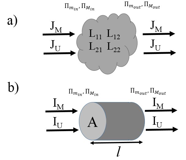
Figure 1: Schematic view of a metabolic device. a) local description of the Onsager unit cell, and b) schematic view of a portion of a living system (where $I_{U/M}=J_{U/M}A$).

To develop an out-of-equilibrium description of the metabolic process, we transpose the phenomenological linear force-flux formalism approach and Onsager’s reciprocal relations. Consider a thermodynamic unit cell (in the general sense), able to exchange both energy and matter with its environment, and where we can assume local equilibrium. As a matter of fact, both the energy and matter fluxes $\mathbf{J}_{U}$ and $\mathbf{J}_{M}$, depicted in Fig. 1, are conserved, but their coupling induces a modification of the potentials $\Pi_{m}$ and $\Pi_{M}$ across the cell.

To account for the fluxes and the forces which derive from the thermodynamic potentials, we extend the Gibbs relation (1) assuming quasi-static working conditions:

$$\mathbf{J}_{U}=\Pi_{m}\mathbf{J}_{m}+\Pi_{M}\mathbf{J}_{M}$$ (6)

where $\mathbf{J}_{U}$ represents the total energy flux; $\Pi_{m}\mathbf{J}_{m}\equiv\mathbf{J}_{Em}$ is the dispersed microscopic energy flux, and $\Pi_{M}\mathbf{J}_{M}$ is the aggregated energy flux, proportional to the power produced on the macroscopic level, such as, e.g, the mechanical power. For a living system, $\Pi_{m}$ is the chemical potential of the digested food, which we denote $\mu$ according to standard notations, so that the equivalent entropy flux is $\mathbf{J}_{S}=\mathbf{J}_{m}/\mu$ and $\Pi_{M}$ is the macroscopic potential from which the muscular force derives. The flux $\mathbf{J}_{M}$ may be seen as the metabolic intensity necessary to maintain a given metabolic state for the living system. For our purpose, we focus on the coupled fluxes $\mathbf{J}_{Em}$ and $\mathbf{J}_{M}$, that can be computed using the force-flux formalism:

$$\left(\begin{array}[c]{c}\mathbf{J}_{M}\\ \mathbf{J}_{Em}\end{array}\right)=\left(\begin{array}[c]{cc}L_{11}&L_{12}\\ L_{21}&L_{22}\end{array}\right)\left(\begin{array}[c]{c}-\frac{1}{\Pi_{m}}\mathbf{\nabla}(\Pi_{M})\\ \mathbf{\nabla}(\frac{1}{\Pi_{m}})\end{array}\right)$$ (7)

The off-diagonal kinetic matrix coefficients satisfy Onsager’s reciprocity relations $L_{12}=L_{21}$ [12]. In the present case of two coupled flows, the Onsager matrix contains four terms that are reduced to three due to the reciprocity resulting from the Le Chatelier-Braun principle. These three parameters are respectively related to the conductivities associated with each of the flows, on the one hand, and the coupling coefficient between flows, on the other hand [30]. For simplicity and with no loss of generality, we consider a one-dimensional description (in $x$-coordinate) and rewrite Eq. (7) as:

$$\left(\begin{array}[c]{c}J_{M}\\ J_{Em}\end{array}\right)=\left(\begin{array}[c]{cc}L_{11}&L_{12}\\ L_{21}&L_{22}\end{array}\right)\left(\begin{array}[c]{c}\phantom{-}\frac{\displaystyle 1}{\displaystyle\mu}F_{M}\\ -\frac{\displaystyle 1}{\displaystyle\mu^{2}}\frac{\displaystyle\mathrm{d}\mu}{\displaystyle\mathrm{d}x}\end{array}\right)$$ (8)

where we introduced the macroscopic driving force $F_{M}=-\mathrm{d}\Pi_{M}/\mathrm{d}x$.

2.3 Transport coefficients

Let us first derive the expression of the isochemical potential conductivity. In this configuration, the chemical potential is constant and the chemical energy distribution gradient within the body vanishes: $\mu$ is constant and $J_{M}=\frac{L_{11}}{\mu}F_{M}$. The metabolic intensity $J_{M}$ is driven by the force $F_{M}=-\mathrm{d}\Pi_{M}/\mathrm{d}x$ which is nothing but the muscular force on the macroscopic level. The metabolic conductivity is then given by

$$\sigma=\frac{L_{11}}{\mu}$$ (9)

The quantity $\sigma$ is the isochemical potential conductivity. It embodies dissipation when the muscles produce a mechanical activity, including locomotion but also any motionless efforts. When considering a segment of muscle of length $l$ and section $A$, one obtains the expression of the dissipative metabolic resistance $R_{M}=l/A\sigma$. Considering the situation when the animal is at rest, with no mechanical activity, we now derive the expression of the basal metabolic conductivity. As the metabolic intensity $J_{M}$ vanishes, the metabolic power flux $J_{Em}^{\ast}$ becomes:

$$J_{Em}^{*}=-\kappa_{J_{M}}\frac{\mathrm{d}\mu}{\mathrm{d}x}$$ (10)

where $\kappa_{J_{M}}=\frac{1}{\mu^{2}}\left[\frac{L_{11}L_{22}-L_{21}L_{12}}{L_{11}}\right]$ denotes the basal metabolic conductivity. Since $J_{Em}^{*}$ is a measure of the consumed power density when the animal is at rest, $\kappa_{J_{M}}$ can be considered as a metabolic conductivity under zero load, from which we define the basal metabolic impedance: $R_{E}=l/\kappa_{J_{M}}A$, still considering a system of length $l$ and section $A$.

Let us now consider the opposite configuration, when the animal experiences an exhausting effort. In this case, the animal dissipates all the mechanical power while producing zero contribution to motion. This situations occurs for metabolic intensities far above the location of the maximal power. The organism is no longer able to sustain the required effort. The net mechanical power transferred to the environment vanishes, so does the net associated mechanical force, i.e. $F_{M}=0$. The entire metabolic power produced by the muscles is consumed within the animal. In other words, the animal metabolism is in the short-circuit configuration, fully loaded, and the metabolic intensity density $J_{M}$ reaches a critical value $J_{X}$ at the exhaustion stage. Then, from Eq. (8), the associated energy flux, denoted $J_{Em}^{\dagger}$, under the zero mechanical condition is:

$$J_{Em}^{\dagger}=-\kappa_{F_{M}}\frac{\mathrm{d}\mu}{\mathrm{d}x}$$ (11)

where ${\displaystyle\kappa_{F_{M}}=\frac{L_{22}}{\mu^{2}}}$ is the exhaustion metabolic conductivity.

One can notice that the link between $\kappa_{F_{M}}$ and $\kappa_{J_{M}}$ derives from the definitions of the transport coefficients:

$$\kappa_{F_{M}}=\kappa_{J_{M}}\left[1+\frac{\alpha^{2}\sigma}{\kappa_{J_{M}}}\mu\right]$$ (12)

This relation shows that the most efficient metabolic conditions are when the basal metabolism is as low as possible while the exhausting metabolism conditions are delayed as long as possible. By “most efficient”, we mean “with a minimal entropy production”, hence maximal possible conversion of the food chemical energy into useful muscular power. The rejected fraction of matter and energy into the sink is here considered as a waste. It is clear that, contrary to the waste heat of steam engine, most of this biological waste should be considered as secondary metabolites for the waste matter, and warming body contribution for the waste energy. All these secondary contributions could be included in a more complex thermodynamic network whose generic building block would be the present Onsager unit cell. A complete analysis of such a complex thermodynamic network is out of the scope of the present paper.

Equation (12) also indicates that the ratio $\kappa_{F_{M}}/\kappa_{J_{M}}$ provides a direct measure of the efficiency of the equivalent working fluid, as we obtain an expression of the metabolic figure of merit, which can be viewed as the biological equivalent of the figure of merit known in the field of thermoelectricity [31]:

$$f_{M}=Z\mu=\frac{\alpha^{2}\sigma}{\kappa_{J_{M}}}\mu$$ (13)

which is the extension of the expression of Eq. (5) beyond the equilibrium state. In the case of a complete system of length $l$ and section $A$ (see Fig. 1b), the figure of merit now reads

$$f_{M}=\frac{\alpha^{2}R_{E}}{R_{M}}\mu$$ (14)

The figure of merit is often defined as the degree of coupling of the fluxes. In their seminal paper, Kedem and Caplan derived the following expression of the coupling parameter between the two fluxes involved in the conversion process [30]:

$$q=\frac{L_{12}}{\sqrt{L_{11}L_{22}}}=\sqrt{\frac{f_{M}}{1+f_{M}}}$$ (15)

which explicitly includes the kinetic coefficients $L_{ij}$. The figure of merit and the coupling factor $q$ are equivalent in terms of measure of the efficiency of the system: the higher their (absolute) values, the better the energy conversion system. This can be evidenced by the derivation of the local maximal efficiency of the conversion process $\eta_{\mathrm{max}}$:

$$\eta_{\mathrm{max}}=\left(\frac{1+\sqrt{1-q^{2}}}{q}\right)^{2}=\frac{\sqrt{1+f_{M}}-1}{\sqrt{1+f_{M}}+1}$$

We observe that the figure of merit $f_{M}$ provides a direct quantitative indicator of the performance of the considered system. Denoting $F_{M_{0}}$ the macroscopic force under the basal metabolism configuration, $J_{M}=0$, the expression of the coefficient $\alpha$ may be rewritten as:

$$\alpha=F_{M_{0}}\left(\frac{d\mu}{dx}\right)^{-1}=\frac{1}{\mu}\frac{L_{12}}{L_{11}}$$ (16)

From the derivation of the transport coefficients, we see that only three transport parameters are required to characterize the metabolic machine: two conductivities, respectively for the aggregated energy flux, $\sigma$, and the dispersed energy flux, $\kappa_{J_{M}}$, and a coupling parameter between these two fluxes, namely $\alpha$.

3 The thermodynamics of metabolism

3.1 The metabolic machine

3.1.1 Local energy budget

Replacing the kinetic coefficients $L_{ij}$ in Eq. (7) by the transport coefficients, $\sigma$, $\kappa_{J_{M}}$ and $\alpha$, yields the following expressions for the fluxes $J_{M}$ and $J_{Em}$:

$$\left(\begin{array}[c]{c}J_{M}\\ J_{Em}\end{array}\right)=\left(\begin{array}[c]{cc}\sigma&\alpha\sigma\\ \alpha\sigma\mu&\kappa_{\Pi_{M}}\end{array}\right)\left(\begin{array}[c]{c}F_{M}\\ -\frac{\displaystyle\mathrm{d}\mu}{\displaystyle\mathrm{d}x}\end{array}\right)$$ (17)

Assuming constant parameters, the gradient of $J_{Em}$ then reads

$$\frac{\mathrm{d}J_{Em}}{\mathrm{d}x}=\alpha J_{M}\frac{\mathrm{d}\mu}{\mathrm{d}x}-\kappa_{J_{M}}\frac{\mathrm{d}^{2}\mu}{\mathrm{d}x^{2}}$$ (18)

Note that the transport coefficients are in general not constant, but the constant transport parameter assumption is routinely used when the potential gradients in a given system are sufficiently small so that the system remains close to equilibrium (or close to some effective quasi-equilibrium). For sake of simplicity the present work focusses on “moderate” efforts, which imply small gradients of the intensive parameters and hence a negligible dependence of the transport coefficients on energy, space and time, as one analyses the production of mechanical force on the global scale. Also, we make the assumption of sufficiently short duration metabolic effort and hence secondary metabolites do not partake in the chemical-to-mechanical energy conversion and are simply considered as waste. In this case, the transport parameters are not affected by the presence of these secondary metabolites.

As energy conservation imposes a constant total energy flux $J_{U}$ in Eq.(6), we get

$$\frac{\mathrm{d}J_{Em}}{\mathrm{d}x}=F_{M}J_{M}$$ (19)

and combining Eqs. (18) and (19), we finally obtain the local energy budget:

$$\kappa_{J_{M}}\frac{\mathrm{d}^{2}\mu}{\mathrm{d}x^{2}}=-\frac{J_{M}^{2}}{\sigma}$$ (20)

One may now notice that although dissipation does not explicitly appear in the force-flux expressions, it does in the local budget equation through the term $J_{M}^{2}/\sigma$. In other words, the conservation of the energy and matter, $\nabla{J_{U}}=0$ and $\nabla{J_{M}}=0$ and the local working conditions of the metabolic device are totally defined by the local budget and the three transport coefficients $\sigma$, $\kappa_{J_{M}}$ and $\alpha$. Let us now extend the analysis to the management of this equivalent working fluid inside an organism or part of it.

3.1.2 Metabolic flux

Assuming that the metabolic processes take place in the volume $A\times l$ of the organism, the complete energy budget is obtained after integration of Eq. (20)

$$\frac{\mathrm{d}\mu}{\mathrm{d}x}=-\frac{J_{M}^{2}}{\sigma\kappa_{J_{M}}}x+C$$ (21)

The energy flux $\Phi=AJ_{Em}$ can hence be expressed as

$$\Phi=\alpha\mu I_{M}-\kappa_{J_{M}}A\frac{\mathrm{d}\mu}{\mathrm{d}x}$$ (22)

where $I_{M}=AJ_{M}$ is the metabolic intensity. This latter is directly related to the average rate of production of the chemical reactions. The metabolic flux now reads from Eq. (19):

$$\Phi(x)=\alpha\mu(x)I_{M}+R_{M}I_{M}^{2}\frac{x}{l}+C$$ (23)

The term $C$ is determined by the boundary conditions at both locations $x=0$ and $x=l$. Now, in order to complete the description of the system and the model, we turn to boundary conditions specification.

3.2 The metabolic system

3.2.1 Metabolic power

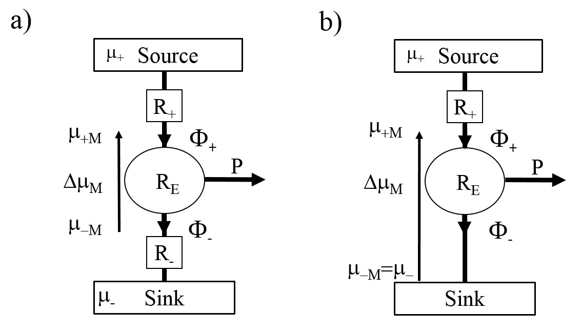
Figure 2: Thermodynamic system: a) general configuration. b) simplified configuration for low-duration, steady-state efforts, with $R_{-}=0$. A dissipative coupling modifies the chemical potential difference across the conversion zone.

As a thermodynamic device, the metabolic conversion zone defined by the element of length $l$ and section $A$ is inserted in a global system. The boundary conditions impose the values of both energy and matter currents and consequently, the working conditions of the metabolic device. The complete thermodynamic system is represented on Fig. 2, which arguably outlines a quite general situation. Due to the presence of dissipative couplings between the conversion zone and the reservoirs, the reservoirs chemical potentials $\mu_{+}$ and $\mu_{-}$ are modified and become $\mu_{+M}$ and $\mu_{-M}$ as shown on Fig. 2.

The metabolic converter is connected to a reservoir and a sink by two dissipative elements of resistances, $R_{+}$ and $R_{-}$. These resistances, together with the basal metabolic resistance $R_{E}=l/\kappa_{J_{M}}A$, allow considering mixed boundary conditions between two limit cases, namely i) the Neumann conditions, where currents are imposed, considering high, diverging values of $R_{+}$ and $R_{-}$; ii) the Dirichlet conditions, where potentials are imposed, considering instead vanishing values for $R_{+}$ and $R_{-}$. It is important to note that the crucial question of boundary conditions is imposed by the system, namely, a metabolic machine contained within a defined perimeter. From a theoretical point of view, it would be perfectly possible to define conditions at Neuman’s limits by considering the organism within its biotope, as a complete system receiving a flow of matter and energy. However, the perimeter of the system, imposed by the body envelope is an unavoidable constraint in this model, and this constraint leads to consider irreducible mixed boundary conditions. From the general expression Eq. (23), we get the expressions of the incoming $\Phi_{+}=\Phi(0)$ and outgoing $\Phi_{-}=\Phi(l)$ fluxes:

$$\Phi_{+} =\alpha\mu_{+M}I_{M}+\frac{\Delta\mu_{M}}{R_{E}}$$ (24)

$$\Phi_{-} =\alpha\mu_{-M}I_{M}+R_{M}I_{M}^{2}+\frac{\Delta\mu_{M}}{R_{E}}$$ (25)

where $\Delta\mu_{M}=\mu_{+M}-\mu_{-M}$. The term $C=\Delta\mu_{M}/R_{E}$ comes from the flow balance at the incoming and outgoing borders of the conversion zone. Accounting for the connections to the reservoirs, we get two additional expressions for the fluxes:

$$\Phi_{+} =\frac{\mu_{+}-\mu_{+M}}{R_{+}}$$ (26)

$$\Phi_{-} =\frac{\mu_{-M}-\mu_{-}}{R_{-}}$$ (27)

that yield the following simple expression for the metabolic converter output power $P$:

$$P=\Phi_{+}-\Phi_{-}=\left[\alpha\Delta\mu_{M}-R_{M}I_{M}\right]I_{M}$$ (28)

The expressions (24), (25), (26), and (27) now give a complete set of equations for a proper description and analysis of a given metabolic situation. The calculation of the general solution does not pose any specific difficulty but is quite tedious.

3.2.2 Chemical-to-mechanical energy conversion parameters

For illustration purposes, let us consider the particular situation of an effort with reasonable (low) duration, neglecting the drawback effects of the waste fractions; in this case, the coupling resistance to the sink $R_{-}$ may be considered as negligible, and $\mu_{-M}\approx\mu_{-}$. We obtain the simplified expressions:

$$\Phi_{+} =\frac{F_{\mathrm{iso}}I_{M}/{\eta}_{\mathrm{C}}+B}{I_{T}+I_{M}}~{}I_{T}$$ (29)

$$\Phi_{-} =R_{M}I_{M}^{2}+\frac{R_{\mathrm{fb}}I_{M}^{2}+{F_{\mathrm{iso}}}\left(\frac{1}{{\eta}_{\mathrm{C}}}-1\right)I_{M}+B}{I_{T}+I_{M}}~{}I_{T}$$ (30)

where all the quantities are defined in Table 2. In order to simplify the identification of the boundary conditions we define the parameter $r=\frac{R_{+}}{R_{+}+R_{E}}$. This parameter varies from $r=0$ when the system is connected with potential boundary conditions, i.e. of the Dirichlet type, to $r=1$ in the case of flux conditions, i.e., Neumann type.

Quantity	Definition
${\displaystyle I_{M}}$	macroscopic (space integrated) metabolic intensity
${\displaystyle I_{M}F_{M}}$	available mechanical power
${\displaystyle B=\frac{\Delta\mu}{R_{+}+R_{E}}=}\frac{\Delta\mu}{R_{E}}(1-r)$	basal power consumed by the body at $I_{M}=0$, or $F=F_{\rm iso}$
${\displaystyle{I_{T}=\frac{R_{E}+R_{+}}{\alpha R_{+}R_{E}}=}}\frac{1}{\alpha rR_{E}}$	threshold metabolic intensity
${\displaystyle R_{\mathrm{{fb}}}=\alpha\mu_{-}/I_{T}=r}\alpha^{2}R_{E}\mu_{-}$	feedback resistance
${\displaystyle F_{\mathrm{iso}}{=\alpha R_{E}B}}$ =$\alpha{\Delta\mu}(1-r)$	isometric force
${\displaystyle\eta_{\mathrm{C}}=\frac{\mu_{+}-\mu_{-}}{\mu_{+}}}$	overall chemical-mechanical machine efficiency

Table 2: Thermodynamic parameters characterizing the chemical-to-mechanical energy conversion.

Note that the product or ratio of some couples of parameters result in constant quantities such as, e.g., $F_{\rm iso}/B=\alpha R_{E}$ and $R_{\rm fb}I_{T}=\alpha\mu_{-}$, which creates some particular constraints. This point will be developed further in the article.

Both $R_{\mathrm{fb}}$ and $I_{T}$ are governed by the boundary conditions for the energy entering the system; in other words, they characterize the ability of the biological system to feed the conversion zone with chemical energy, this ability being limited by the coupling resistance $R_{+}$. Note that if the boundary conditions would only be of the potential type (Dirichlet conditions), the feedback resistance $R_{\mathrm{fb}}$ would be zero. We discuss the importance of the feedback resistance for muscle work in the frame of Hill’s model in the next section, as $I_{T}$ corresponds exactly to one of Hill’s constants, and $R_{\mathrm{fb}}$ is instrumental to elucidate the question of the non-constancy of Hill’s first “constant” $a$ (defined in the next Section).

The metabolic power delivered during a physical effort is expressed as:

$$P=\Phi_{+}-\Phi_{-}=F_{M}I_{M}=\left[{F_{\mathrm{iso}}}-\left(R_{M}+R_{H}(I_{M})\right)I_{M}\right]I_{M}$$ (31)

where $F_{\mathrm{iso}}$ is the so-called isometric force [32], which describes the situation of a muscle tension under load but with no motion, and where the resistance $R_{H}(I_{M})=\frac{{F_{\mathrm{iso}}}+R_{\mathrm{fb}}{{I_{T}}}}{I_{T}+I_{M}}$ is introduced as a metabolic intensity-dependent resistance showing clearly that the organism cannot be seen as a passive system in the sense that it does not merely represent a system component that merely dissipates energy as a standard resistor would in an electrical circuit. In the present model, $R_{M}$ acts as such a passive component. On the contrary, the definition of $R_{H}$ contains $R_{\mathrm{fb}}$, and both can be expected to stem from feedback effects. They are thus tightly related, notably through the threshold metabolic intensity.

With Eq. (31), we also recover the classical expression of a force-intensity response, with the isometric force ${F_{\mathrm{iso}}}$ and the composite internal resistance $R_{H}(I_{M})+R_{M}$. As expected, the isometric force is proportional to the converted fraction of the chemical energy difference $\Delta\mu$ modulated by the resistance bridge value: $\frac{R_{E}}{R_{+}+R_{E}}$. Furthermore, as the composite resistance $R_{H}(I_{M})+R_{M}$ depends on the metabolic intensity, we see that it may govern the shape of the response curves of a muscle, which is quite a central result, as will be shown later.

The output power accounts for the power spent to sustain the physical effort balanced by the dissipated power. It is important to note that the notion of “physical effort” may encompass a quite large variety of efforts. In the case of an animal in motion, at velocity $v$, the physical effort simply corresponds to the production of the mechanical power necessary for actual motion. In this case, the metabolic intensity can be expressed directly from the rate of production of chemicals [33] and, consequently, the mechanical velocity of the system as $I_{M}\equiv kv$, where $k$ is a dimensional constant. But the metabolic intensity is also non-zero for animals carrying heavy loads, while standing still. Further, the power $P$ has two zeros, corresponding to two specific values for the intensity: $I_{M}=0$ in the absence of any effort, and $I_{M}=I_{X}$, the maximum value of intensity at $P=0$, in a situation of exhaustion with $I_{X}=\frac{{F_{\mathrm{iso}}}}{R_{H}+R_{M}}$. Therefore, the concept of metabolic intensity accounts for various types of efforts, that a purely mechanical description cannot.

Turning to the figure of merit, we see that it now reads

$$f_{M}=\frac{R_{\mathrm{fb}}F_{\mathrm{iso}}I_{T}}{R_{M}B}$$ (32)

We thus obtain a compact expression which, while preserving its thermodynamic structure, can be read in a form directly accessible to the understanding of metabolic performance. Let us analyse what are the compromises and expectations at stake for a given value of this merit factor. First of all, it is clear that mechanical power is only available as much as the mechanical viscosity $R_{M}$ makes it possible. Similarly, we can notice the presence of the $F_{\mathrm{iso}}/B$ ratio which reflects the necessary compromise between the availability of force and the “basal” dimension of the machine that leads to this availability. Last, the product $R_{\mathrm{fb}}I_{T}=\alpha\mu_{-}$ which can be considered constant, shows us that the metabolic intensity is necessarily contingent on the feedback resistance, and that high metabolic intensities can only be achieved by a significant reduction in this resistance.

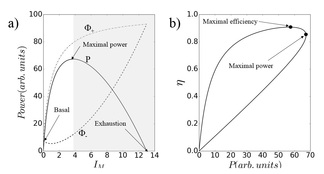
Figure 3: a) Generic power plots: external mechanical power $P$ (straight line), input $\Phi_{+}$ (dash-dotted), and output $\Phi_{-}$ (dash) metabolic fluxes. The shaded area corresponds to the region where the organism degrades more mechanical power than it uses for the effort. b) Efficiency versus power response. As the metabolic intensity $I_{M}$ increases, the efficiency $\eta$ reaches its maximum before the mechanical power reaches its own maximum.

It is important to note that $f_{M}$ does not depend on the ratio $r=R_{E}/(R_{+}+R_{E})$; in fact, it is a quantity that intrinsically characterizes the thermodynamic conversion capacity, regardless of the coupling conditions to the reservoirs. Finally, using the set of equations (29), (30) and (31), we can now plot the generic response of an organism to an effort as shown on Fig. 3a where the input ($\Phi_{+}$), output ($\Phi_{-}$) and mechanical ($P=\Phi_{+}-\Phi_{-}$) powers are reported. We also plot on Fig. 3b the efficiency $\eta=\frac{\Phi_{+}-\Phi_{-}}{\Phi_{+}}$ vs power curve: the maximal efficiency is obtained for a metabolic intensity substantially below that required for the production of maximal mechanical power, while the mechanical output is only slightly below the maximal one. The latter is reached at the cost of efficiency. It can easily be shown that the higher the $f_{M}$ factor, the further away the maximum efficiency and maximum power points shall be apart. This confirms that there is no optimal operating point in absolute terms, let alone an underlying general variational principle. Depending on the metabolic parameters, each muscle is subjected to a trade-off between its maximal efficiency and its maximal power, or minimum production of waste. We shall discuss the question of the variational principle in Section 5. We show that the biological system becomes obviously deterministic at the condition that the system definition properly includes the boundary conditions.

4 Metabolic energy conversion under muscle load

4.1 Physical efforts

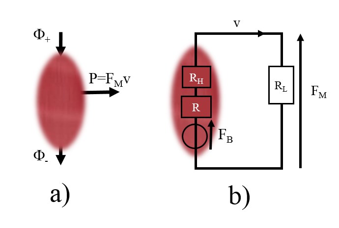
Figure 4: Thermodynamic to mechanical conversion: a) Metabolic power conversion; b) Mechanical power production.

Let us now consider the muscular strength deduced from the expression of power by simply writing $F_{M}=P/I_{M}$. As previously mentioned, using the above formalism, we can identify the force from an equivalent generator scheme, including in series the isometric force $F_{\mathrm{iso}}$ and the internal resistance $R_{M}+R_{H}(I_{M})$. It follows that Figure 4 summarizes the principles of the thermodynamic model of metabolic power generation, i.e. energy conversion from chemical power to mechanical power, in the case of short-duration efforts. The complete system is composed of two parts. The first one (a) is the biochemical converter, which receives the incoming chemical power $\Phi_{+}$, delivers an output power $P$, and produces waste and secondary metabolites, denoted $\Phi_{-}$. In b), the mechanical power $P$ is partly dissipated within the organism because of “friction” due to the internal composite resistance $R_{M}+R_{H}(I_{M})$, where the latter contribution corresponds to the variable part of the dissipative mechanism. Without going into details that are beyond the scope of this article, we observe that this non-linear mechanical resistance is an active impedance in the sense that it depends on the metabolic intensity, and hence on the operating point of the system. This is a major and principle departure from passive models that traditionally take this restrictive assumption on this impedance. Moreover, several experimental studies based on the frequency-dependent linear response of this impedance [34, 35, 36, 37], show a resonant frequency response. In the presence of a feedback, such a resonance is quite possible since the response of the closed-loop system may present an even higher order response than that of an open loop system [16]. At this stage of the description, it becomes important to compare the model and its predictions with a well-defined biological system. To do so, we consider the case of skeletal muscle in the frame of Hill’s approach.

4.2 Revisiting Hill’s muscle load model

Assuming that the entire metabolic power produced is converted into mechanical power, we may write $P=F_{M}I_{M}$, and using Eq. (31), we find:

$$F_{M}=\frac{\left(F_{\mathrm{iso}}+R_{\mathrm{fb}}I_{T}\right)I_{T}}{\left(I_{M}+I_{T}\right)}-\left(R_{\mathrm{fb}}I_{T}+R_{M}I_{M}\right)$$ (33)

This expression is the thermodynamics-based formulation of the force response in presence of an effort of intensity $I_{M}$. We now turn to the comparison with the model proposed by Hill in 1938 [9], which is the most classical muscle description for chemical-to-mechanical power metabolic conversion, and thus serves here as a touchstone. In his seminal article based on dynamic calorimetric measurements, Hill assumed that the chemical energy rate was proportional to the contraction velocity $v$ of the muscle, and consequently that: $I_{M}\propto v$. In other words he proposed to switch from thermodynamic arguments to mechanical ones (see A). Hill’s state equation reads:

$$F_{M}=\frac{c}{\left(v+b\right)}-a\noindent$$ (34)

From Eq. 33 we unambiguously identify

$$a=R_{\mathrm{fb}}I_{T}+R_{M}I_{M}\noindent$$ (35)

$$b=I_{T}\noindent$$ (36)

$$c=\left(F_{\mathrm{iso}}+R_{\mathrm{fb}}I_{T}\right)I_{T}\noindent$$ (37)

Besides the similarity of Eq. (33) and Eq. (34) it is important to consider how to give Hill’s model a proper thermodynamic ground. In this spirit, we propose to consider four questions that mark the history of the Hill model and that turn out to find a common framework here: i) the chemical origin of part of the observed mechanical dissipation; ii) the presence of slow and fast muscle fibres, iii) the rectilinear versus non-linear shape of the force-velocity measurements, and, finally iv) the speed dependence of the so-called extra heat term $a$.

4.2.1 Chemical origin of parameter $a$

The principal elements of Hill’s model are summarized in A; the model shows that a chemical contribution to dissipation during muscle contraction was a central hypothesis of the muscle model [9], and as such, had been added to the energy budget. This point had first been raised by Fenn who claimed that the fact that an active muscle shortens more slowly under a greater force, is not due to mechanical viscosity but to how the chemical energy release is regulated [38, 39] (see also the critical analysis of Fenn’s works in [40]). Both Fenn and Hill did not make use of any feedback effect between chemical input and mechanical output. However, considering the expressions of $R_{\rm fb}$ and $I_{T}$, the chemical origin of $a$ is evident. In 1966, Caplan conducted a similar analysis, but the work done considered the local feedback to be an exogenous additional process, without any hint to a change in boundary conditions applied to a macroscopic size system [41]. The influence of modified chemical conditions can also be found in [42] and [43].

4.2.2 Fast and slow fibers

In his Nobel lecture Hill put forth the central question of the fast and slow muscle fibers [11]:

“The difference in the time-scales of the two types of muscle makes one regard it as improbable that physical viscosity alone is the determining factor. One cannot see why viscosity should have ten times the effect in a human muscle than it has in a frog’s, and probably one hundred or one thousand times as much as it has in a fly’s.”

From a mechanical point of view there is no reason why a machine should be constrained by limitations as long as it is able to receive and convert energy, such as chemical energy, into mechanical energy. On the other hand, from the point of view of thermodynamics, the situation is quite different. Indeed, since the performance of the conversion machine is defined both by the thermodynamic fluid and by the machine that uses this fluid, it follows that the maximum performance is limited by the intrinsic capacity of the fluid to carry out the energy conversion. The constant figure of merit $f_{M}=\frac{R_{\mathrm{fb}}F_{\mathrm{iso}}I_{T}}{R_{M}B}$ reflects these intrinsic performances. For a general thermodynamic system there is a figure of merit that defines the upper limit of the performance of the conversion to useful work. This limit can be approached but never exceeded. The situation here is strictly similar and there is therefore a trade-off as to the values of the different parameters. The performance of a muscle is then bounded from above by the figure of merit, that defines the maximum thermodynamic conversion capacity, and consequently, the maximum intrinsic efficiency. To this must be added the constraints that link some of the parameters that make up the figure of merit, namely: $F_{\rm iso}/B=\alpha R_{E}$ and $R_{\rm fb}I_{T}=\alpha\mu_{-}$, which are considered constant. Indeed, in the present case of the response to a time-limited effort, the intrinsic parameters $R_{E}$, $\mu_{-}$ and $\alpha$ are constant.

Let us now consider the specific case of a so-called fast muscle and observe the constraints imposed by the metabolic model. In this case it is expected that the force does not collapse at high speed $v$, i.e. for high values of metabolic intensity close to $I_{T}$. In view of the above remarks, this implies that $R_{\rm fb}$ is minimal, and then so is $R_{+}$. This leads to an increase in the basal power $B$ and therefore an increase in the isometric force $F_{\rm iso}$ by the same amount. Therefore, it appears that fast fibres are also those with the highest isometric forces, and as such are the most powerful fibers, which benefit from little-constrained access to the resource since $r\ll 1$. This double signature is indeed encountered in the case of fast fibres, which are highly energy consuming, even at low speeds, and in particular at the basal level [44, 45]. Then the performance is achieved at the cost of maintaining a substantial basal power that has a definite energy cost which in turn reduces the overall efficiency. On the contrary, in the case of slow fibres, the stress on large $I_{T}$ values is released which leads to a higher $R_{\rm fb}$ resistance and finally a moderate basal power. Note that at birth, some mammals have a very high proportion of slow muscles [44], which tends to decrease as they grow. Such a signature at birth is in accordance with the main property of slow muscles which is their low basal consumption. The same conclusions can be found in the works of Ruegg [46] and Clinch [47].

The difference in the respective values of the basal consumption of fibres and their contraction rates is commonly reported in the literature. As an example we cite the case of the muscles “extensor digitorum longus” and “soleus”, which in mice have contraction rate ratios of 5.9/2 $\simeq$ 2.95 and basal consumption in the ratio 4/1.3 $\simeq$ 3.08 (a value quite close to 2.95) [20, 48, 49]. Since the basal power does not contribute to the production of mechanical power, the choice of slow fibres, when they are sufficient to achieve the function, becomes obvious. From the point of view of glucose combustion, the glycolitic pathway is incomplete since it does not include a Krebbs cycle. The similarity with complete or incomplete combustion of alkanes in internal combustion engines, is quite natural, the efficiency ceiling being in both cases set by the figure of merit of the fuel under total combustion conditions. In other words, one may observe that the overall performance of the muscle is, as in the case of any thermodynamic system, the result of a trade-off between the intrinsic combustion properties of the fuel on the one hand, and the implementation of this combustion according to a particular path imposed by the machine, on the other hand. Similarly, we can see that in the case of muscles of the same nature, ($r$ constant) the ratio $a_{0}/F_{\rm iso}$ is predicted to be constant, which is actually reported in [44]. Although temperature is not explicitly present in our model, the influence of a muscle temperature during exercise is easily visible on the measurements [50]. The general shape of the curves is not globally modified, but the parameters have a sizable temperature dependence.

4.2.3 Linear and non-linear shape of the force-velocity curves

It is known that slow and fast fibres do not have the same force-speed response. If the classic form of the force-speed response according to Hill is that of a hyperbola, mention has been made of responses with a very shallow, or even totally rectilinear, character [42, 44, 45]. The existence of linear characteristics means that in these cases the dissipation resistance $R_{H}(I_{M})+R_{M}$ is almost constant. As a result, the term $R_{H}(I_{M})$ is no longer a function of the current $I_{M}$. This amounts to considering that $I_{T}\gg I_{M}$. It follows that the predominance of fast fibres leads to more linear characteristics. This was indeed observed for the human in the force-speed response of the arms [51]. Physiological analyses reveal the predominance of fast fibres in the arms, unlike legs which have more slow fibres. This is true in general for the untrained individual. In the case of sprint-trained runners [52] or cyclists [53], there is a strong tendency towards the linear form, which in these cases reflects the predominance of fast fibres, as predicted by the model. The same signature is obtained if the pedalling is done with the arms [54].

We can illustrate the dependence of the boundary conditions connection quality (value of $r$) according to the fibre types by using data on EDL and soleus muscles [44]. These latter are distinguished by their fraction of fast and slow fibres, which in our formalism translates as a better coupling to the reservoirs, and hence: $r_{\rm{SOL}}<r_{\rm{EDL}}$. Further, by normalizing the force by the isometric force, $F_{\rm{iso}}$, in Eq. (33), and the velocity by the short circuit velocity, $v_{X}$, we obtain the following expression:

$$\frac{F}{F_{\mathrm{iso}}} = \zeta(r)\frac{1-v/v_{X}}{v/v_{X}+\zeta(r)}-\frac{R_{M}v_{X}}{F_{\mathrm{iso}}}\frac{v}{v_{X}}$$ (38)

with $\zeta(r)=\frac{a_{0}}{F_{\mathrm{iso}}}=\frac{a_{0}}{\alpha\Delta\mu}\frac{1}{1-r}$ and $\frac{a_{0}}{\alpha\Delta\mu}$ constant. The first term corresponds to the force-velocity response in the absence of contribution of the mechanical dissipation, i.e., $R_{M}=0$. We then obtain an expression whose only degree of freedom is $r$. In other words, one can only distinguish a fast fibre from a slow fibre, or two muscles composed of a different fraction of each other, by their dependence on boundary conditions. The presence of mechanical dissipation ($R_{M}\neq 0$) results in a correction for the higher velocity: for a given velocity, the available force is reduced.

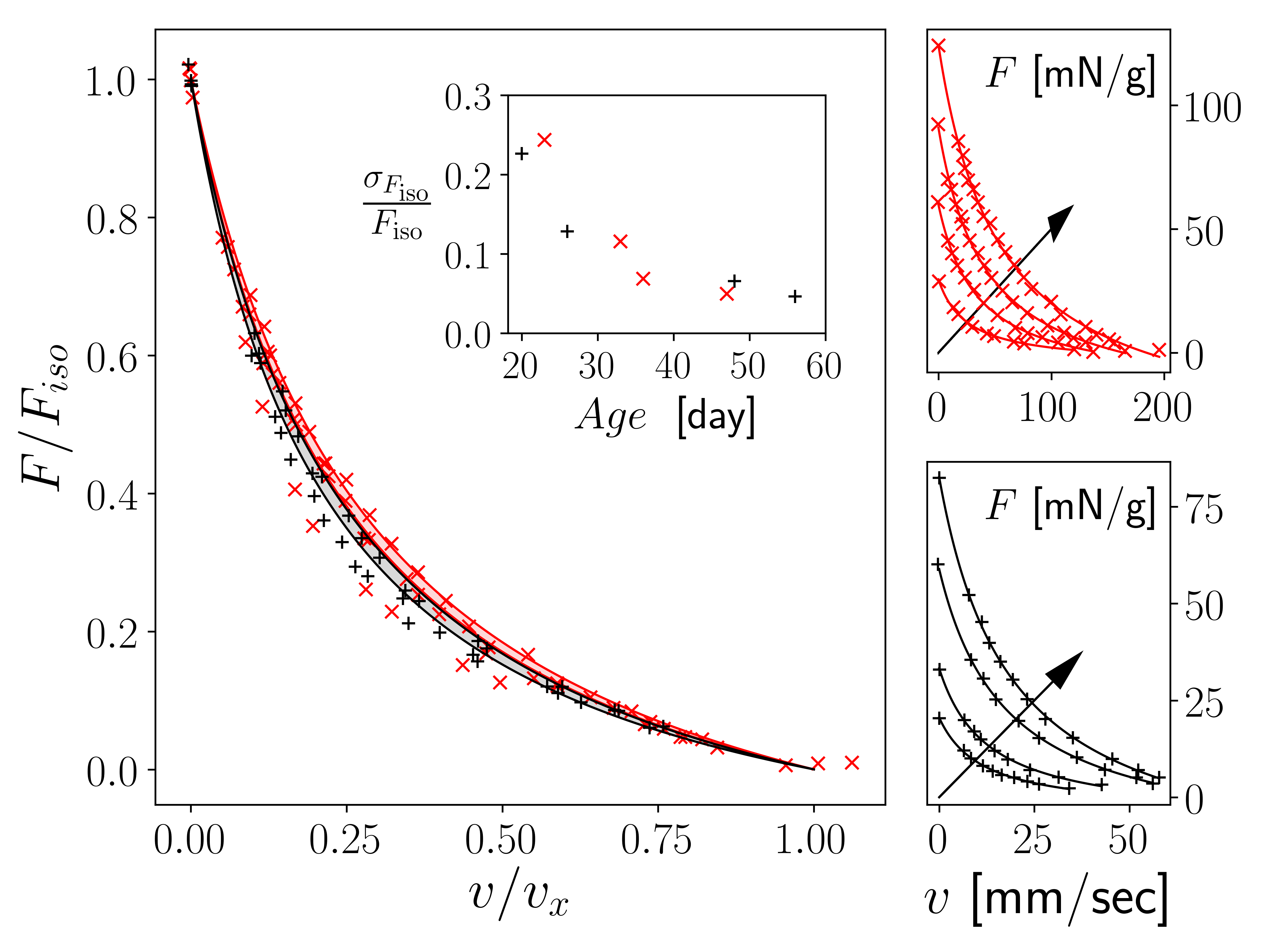
Figure 6: On the right panel, we show the data extracted from [44]. Top is force-velocity response for the extensor digitorum longus (EDL, red $\times$) and bottom is soleus (SOL, dark $+$) of female rats for various ages (resp. 23, 33, 36 and 47 days, and 20, 26, 48 and 56 days). In both cases, age increases in the direction of the arrow. Lines are respective best fits, from Eq. (34) without dissipation ($R_{M}=0$ or $a=a_{0}$). The corresponding relative uncertainty of $F_{\rm iso}$ compared to the age of the muscle is represented on the inset of the left panel. On the left panel is shown the corresponding normalized force-velocity response for EDL and SOL using the same color and symbol codes. Normalization is obtained by extracting for each set of data the respective force $F_{\rm iso}$ and velocity $v_{x}$, which is the maximum velocity at $P=0$. The respective shaded areas correspond to curve fitting, based on Eq. (38), which also takes into account uncertainties (see inset) in data extraction and curve fitting of the force-velocity response.

The panels on the right side of Fig. 6 show experimental data on the EDL and soleus muscles [44], in a force-velocity representation. The fits shown are based on Hill’s equation without direct contribution of the mechanical dissipation, for which $R_{M}=0$ and $a=a_{0}$; this hypothesis makes it possible to fit the experimental data with very good agreement. In the following, we limit the scope of our analysis to this configuration.

The experimental data normalized by the isometric force, $F_{\mathrm{iso}}$, and the short circuit velocity, $v_{X}$, obtained for each of the previous fit are reported on the panel left of Fig. 6. The fits of these data are also done with Eq. 38 under the assumption of mechanical dissipation. The uncertainty of the experimental data was estimated at 1/4 of the marker size. We observe in the inset of Fig. 6 that both relative and absolute uncertainties decrease sharply with the age of the muscle. Consequently the data obtained for the oldest ages are dramatically more weighted in the fitting process. The shaded regions represent the best fit of the normalized and aggregated data for each muscle at plus and minus one standard deviation. We then have $\zeta_{\rm{EDL}}=0.27\pm 0.02$ and $\zeta_{\rm{SOL}}=0.23\pm 0.02$, which verifies that $r_{\rm{SOL}}<r_{\rm{EDL}}$. By recognizing that $\frac{\zeta_{\rm{EDL}}}{\zeta_{\rm{SOL}}}=\frac{1-r_{\rm{SOL}}}{1-r_{\rm{EDL}}}$, we obtain the condition $r_{\rm{EDL}}\geq 1-\frac{\zeta_{\rm{SOL}}}{\zeta_{\rm{EDL}}}$. A strict equality in the latter expression would imply that $r_{\mathrm{SOL}}$ is exactly zero, i.e., the soleus muscle is under the Dirichlet boundary condition. Based on the experimental data, we can therefore conclude, with $r_{\rm{SOL}}>0$, that $r_{\rm{EDL}}>0.14\pm 0.08$.

4.2.4 Speed-dependence of the extra heat term

In his seminal work [9] Hill identified the three parameters as constants, following the viscoelastic origin of the muscle response proposed by Gasser and Hill [55]. As indicated in the appendix, Hill’s 1938 model is based on two hypotheses, one of which concerns the heat released during muscle contraction, which Hill proposed to formulate as proportional to the rate of contraction, $H=av$, where $a$ is the so-called extra heat coefficient considered to be constant. Interestingly enough, this dependence, initially ignored by Hill was considered by Fenn [38, 39, 56], and later reconsidered in experiments by Aubert [57, 58], and finally taken up by Hill himself [10]. A review of these effects can be found in [59, 60]. Indeed, the correction on this term is very generally small, which very often leads to not detecting it experimentally. However, if we consider the complete expression proposed in Eq. (35), we note that the corrective term involves the resistance to mechanical displacement $R_{M}$, which corresponds to the viscosity opposing the displacement of the strands within the muscle fibers. This results in a corrected expression of type $H=aI_{M}+R_{M}I_{M}^{2}$. This correction, although small, is in no way incidental because neglecting it amounts to assimilating, from a mechanical point of view, the muscle fibre to a generator without internal resistance, which could therefore lead to an infinite speed displacement and an equally infinite power production. In practice this situation is not realized because this resistance is in series with the feedback resistance $R_{\rm fb}$ which overrides $R_{M}$ in the mechanical viscous dissipation, which leads to masking the effect of $R_{M}$. From an experimental point of view, by relying on Eq. (35), it is easy to consider the situations for which this corrective term becomes visible. To do this, it is important that the metabolic intensity, and therefore the rate of contraction, can reach high values. This is only possible in cases where $I_{T}$ itself is important, i.e. in the presence of a dominant presence of fast fibres. In this case, the hyperbolic form of the response of the force-speed response curve gives way to a much more rectilinear profile, especially at high velocities as previously described.

The above developments show that it is possible to describe the process of converting chemical energy into mechanical energy in the same terms as any thermodynamic machine composed of a working fluid with a figure of merit, on the one hand, and a device that implements this working fluid on the other hand. In this case, glucose degradation remains the central element to which a figure of merit can be associated. Depending on the coupling conditions to the reservoirs governed by $R_{+}$, this degradation can occur quickly or slowly (glycolytic or oxidative route). More precisely, the kinetic of the glucose combustion, fast or slow, requires the presence of direct $(r\approx 0)$, or reduced, $(r\approx 1)$ access to the resource. But $r$, hence $R_{+}$, does not account for glucose combustion kinetics rate itself, but the latter is compatible only with certain values of $r$. In other words, there is no use to have an efficient device if it is not correctly fed. It could be argued that in this case the condition of direct access to the resource $(r\approx 0)$ should apply systematically since it would ensure a sufficient energy start for any type of muscle, but this is not the case as for slow fibres it would lead to unnecessarily high basal consumption. Our present model does not claim to explain the detailed metabolic pathways, which have been the subject of much work, but rather to characterize the chemical-mechanical conversion through a systemic approach. If by its fast kinetics, inherited from Dirichlet coupling conditions, the glycolytic pathway allows both force and power production, its high basal consumption is nonetheless incompatible with a prolonged effort. On the other hand, due to its Neumann coupling condition, the oxidative pathway exhibits a strong reduction in basal power, allowing a prolonged muscle activity at low power. Therefore, the glycolytic and oxidative pathways are perfectly adapted to the boundary conditions to which they are subjected.

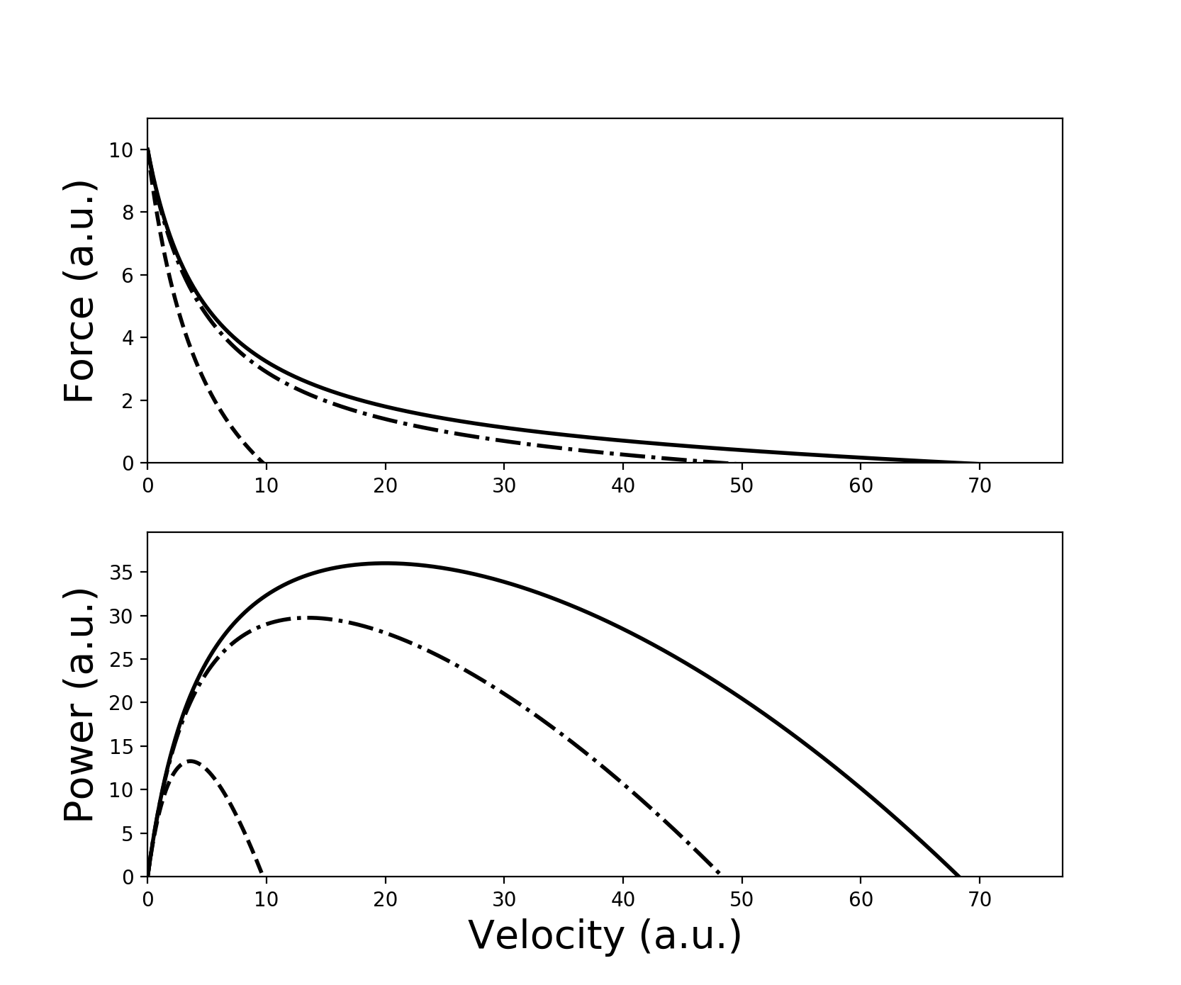
Figure 5: Force-velocity, and power-velocity, response. The three curves differ only in the boundary conditions given by the values of $r$: $0.05,0.15,0.45$ ranging from fast fibres majority to slow fibres majority muscle (see Table 2 for expressions). The line dot curves give the response vs shortening velocity for constant $a_{0}$, i.e., 1938 historical Hill model [9]. The solid line gives the response for non constant $a$ parameter, as reported by Hill in 1964 [10, 58], and shows reduced performances as predicted with our modelling.

As mentioned above, the model only considers short-term efforts and, as such, does not take into account the influence of waste $(R_{-}=0)$. This model can be applied to force-velocity response measurements that are mainly performed under these conditions. An extension of the model to the case of prolonged efforts is of course possible, but the variation of the parameter $\mu_{-}$ would have to be accounted for, which, for simplicity, has not been the case in this article. In Fig. 5 the force-velocity response is displayed for various ratios of the boundary conditions parameter $r$. For a given value of the figure of merit, the variation of $r$ alone is sufficient to produce the slow or fast muscle response curves, while the second figure reproduces the shape of the power curves as they were estimated from Hill’s initial 1938 model and then from his corrected 1963 model, which coincides with our model. Similar result can be found in [58]. The figure represents the relative influences of the composite resistance $R_{H}(I_{M})+R$. In the most classic case $R_{\rm fb}\gg R_{M}$ and the muscle response follows Hill’s initial hyperbolic law. Since $R_{M}$ has a very small value, the feedback term $R_{\rm fb}$ drives the overall response and the dissipation appears to be controlled by the boundary conditions. Otherwise, if $R_{\rm fb}<R_{M}$ then the response becomes linear. This case of high mechanical friction $R_{M}$ would correspond to a particularly low figure of merit, which is unlikely in living systems. Although linear, this response cannot be confused with the response of fast muscles, which are characterized by high values of $I_{T}$. In term of Hill parameters, by noting that $F_{\mathrm{iso}}=c/b-a_{0}$ where $a_{0}=R_{\mathrm{fb}}I_{T}$ it comes that $R_{H}(I_{M})=c/b(b+I_{M})$, and hence

$$P=\left[\frac{c}{I_{M}+b}-a\right]I_{M}$$ (39)

so the maximal intensity is given by, $I_{X}=c/a-b$, which, assuming $a\approx a_{0}$, reduces to

$$I_{X}\approx\frac{F_{\mathrm{iso}}}{R_{\mathrm{fb}}}.$$ (40)

We observe here that, although Hill’s hypothesis, $H=av$ is tantamount to totally neglecting mechanical viscosity, i.e., $R_{M}$ in his description of the muscle (which is a daring hypothesis), this has not had any significant consequence because the dynamics of the system is limited by $R_{\rm fb}$ which dominates and defines the breaking point $I_{X}$.

5 The maximal power principle revisited

In this last section, we show how, within the framework of our approach, the so-called “maximum power principle”, frequently invoked in biology, can be understood as a specific configuration of an out-of-equilibrium system, and should not be considered as a fundamental principle. The capacity of out-of-equilibrium systems to absorb energy was discussed by Lotka [61, 62, 63], before a proper framework for nonequilibrium thermodynamics was put on firm grounds. As recently mentioned by Sciubba [64], Lotka’s assumption referred to the capacity of a given system to maximize the capture of free energy, which is also the free energy fraction of the incoming energy. As it is shown below, Lotka’s description can in fact be reconsidered in terms of impedance matching. However, some misunderstanding of Lotka’s analyses gave rise to the so-called maximal power principle (MPP), which is sometimes considered as the fourth principle of thermodynamics. But, strictly speaking, up to now, the MPP never received final rigorous proof [65, 66, 67, 68, 69, 70]. On the contrary, there is now an increasing consensus to describe out-of-equilibrium systems not in terms of MPP, but simply using the classical principles of thermodynamics, now accounting for specific boundary conditions [15].

We now reconsider this question in the light of the results of our modelling, using the generic picture of Fig. (2). Following Lotka, we consider free energy circulation. A straightforward analysis of the system reveals that the free energy can be destroyed according to three different processes: i) the incoming energy quality is degraded by the presence of $R_{+}$; ii) the basal metabolism is governed by $R_{E}+R_{+}$, which reduces the available free energy for other activities; iii) the internal dissipation term $R_{M}$ diminishes the maximal accessible power. To reduce the effects of these dissipation sources, we may first consider a configuration where $R_{+}=0$, although this assumption is obviously unrealistic. The equation (31) then becomes $P=\alpha I_{M}\left(\mu_{+}-\mu_{-}\right)-R_{M}I_{M}^{2}$ and this means the animal activity would be only limited by its internal dissipation $R_{M}I_{M}^{2}$. In addition, the basal metabolism term $B=\frac{\mu_{+}-\mu_{-}}{R_{E}+R_{+}}$ increases to its maximal value. In other words the gain obtained by easier access to the resources, stemming from the assumption $R_{+}=0$, is counterbalanced by an increase of the basal metabolism. Such a simple extremal free energy analysis is far from being sufficient to explain the optimal physiological point, if any.

Since the condition $R_{+}=0$ is clearly unrealistic, we now turn to the two other cases with $R_{+}\neq 0$. According to the process ii) above, a reduction in the basal metabolism would improve the free energy proportion. Then, in the configuration where $R_{+}$ is small and $R_{E}/R_{+}\ll 1$, Eq. (31) now gives $P\approx\alpha I_{M}\frac{R_{E}}{R_{+}}\left(\mu_{+}-\mu_{-}\right)-R_{M}\left(\frac{\alpha^{2}R_{E}}{R_{M}}\mu_{-}+1\right)I_{M}^{2}$ which means that the available power is vanishingly small, a totally useless configuration. It then becomes obvious that the reduction of the basal metabolism under a certain threshold is not desirable, unless it is imposed by external constraints, such as (and often mainly) food resources. In this respect, as previously described, slow and fast fibers strategies represent two opposite configurations. In short, in order to reach an optimum, a trade-off between the relative values of $R_{E}$ and $R_{+}$ is unavoidable. Clearly, the implicit variational principle for an free energy maximum is necessary but not sufficient, and the feedback induced by the boundary conditions leads to a distribution of the free energy degradation locations [16]. The final distribution depends on the degrees of freedom of each system component, and sub-optimal configurations may exist due to the absence of any degree of freedom on the local level. From a statistical point of view, it is clear that a complex system, composed of a network of diverse engines, may present different (sub)optimal configurations. There exists a constrained matching of the global impedance of the system, allowing an “optimal”, but not necessary maximal, free energy flow.

Let us finally discuss the question of the extremal principle, by deriving an impedance expression. The energy flux is approximately $\Phi\approx{\frac{\mu_{+}-\mu_{-}}{R_{E}+R_{\Sigma}}}$, where $R_{\Sigma}=R_{+}+R_{-}$, and the chemical potential difference $\Delta\mu=\mu_{+}-\mu_{-}$ directly governs the output power. Note that strictly speaking $\Delta\mu=0$ correspond to the dead body condition. Using the argument of the minimization of the degradation of the free energy, we expect a minimization of $R_{\Sigma}$. In addition, if the ratio $R_{E}/R_{\Sigma}\rightarrow 0$, we see that $\Delta\mu_{M}\rightarrow 0$ and both the output power and the efficiency vanish. Now, if we consider the situation where $R_{E}/R_{\Sigma}\rightarrow\infty$, the efficiency becomes maximal, but the power again vanishes. In both cases, we experiment a minimal power principle, with maximal or minimal entropy production. If we now consider $R_{\Sigma}=0$, then the value of $R_{E}$ does not matter any more, and the output power will be maximal, possibly diverging if $R$ decreases. This configuration sounds very similar to the so-called MPP configuration, and actually is, but, as said above, the boundary condition $R_{\Sigma}=0$ is not realistic. If we finally consider that $R_{\Sigma}$ is small but non zero, then the non vanishing $\Delta\mu$ condition imposes a non-zero value for $R_{E}$. Using elementary algebra, the optimal configuration is found to be $R_{E}=R_{\Sigma}$, where the output power is now maximal. If $R_{E}>R_{\Sigma}$ the process favors the energy conversion efficiency at the expense of power; conversely, if $R_{E}<R_{\Sigma}$ the process favors the output power at the expense of efficiency. Therefore, there is no extremal principle for such out-of-equilibrium systems, but there exists a perfectly definite configuration, specified by the actual conditions imposed at the system boundaries.

6 Concluding remarks

Thermodynamics of biological systems entails a rather wide range of problems and models, and remains a very active and timely field of research [71]. In this article, our focus was on the development of a theoretical framework based on a generalized meta-formulation of linear non-equilibrium thermodynamics to characterize the production of metabolic energy and its use under muscular effort. We show that the feedback effects in biological systems permit an analysis based on a local linearized model [16], and starting from the first and second principles of thermodynamics, considered in the context of a locally linear out-of-equilibrium response, we proposed a model of the thermodynamic response of an organism under effort, that lies on a reduced (effective) set of physical quantities: the feedback resistance $R_{\mathrm{fb}}$, the basal power $B$, the isometric force $F_{\mathrm{iso}}$ and the metabolic figure of merit $Z\mu$, which we derived from the generalized thermoelastic and transport coefficients. To actually test the validity of this approach, we used Hill’s model as a touchstone in the sense that through the analysis of Hill’s phenomenological equation we could first establish a direct correspondence with the thermodynamic model and also specify the thermodynamical meaning of Hill’s parameters $a$, $b$, and $c$, including the non-constant behaviour of $a$.

Hill’s phenomenological model derives from calorimetry measurement data [9] and, as such, the force-velocity response formula, Eq. (42), is essentially empirical. In the present work, we made it a principles-based model and we reconsidered many of the questions and debates that have marked its history, some of which finding here a common framework. The main finding of our approach is the active output impedance, that explains the velocity dependence of Hill’s coefficient $a$ (the so-called “extra heat”). This dependence stems from feedback only. There is no fundamental reason why the active impedance would be simply resistive (i.e. a real number); as a matter of fact, it is a complex quantity with a non-zero imaginary part. The standard models proposed since Hill’s seminal work contain a complex impedance, but it is a passive one. Although experimental measurements of muscle response exhibit an overshoot in the frequency space, this overshoot cannot be explained assuming a passive impedance model. Note that it has been established [16] that this type of response may exist if the figure of merit is large, and at the condition that the boundary conditions are of the mixed type, which implies feedback effects and hence an increase of the order of the transfer function of the looped response with respect to the open loop.

Appendix A Hill’s calorimetry developpement

In his seminal article Hill presented an extensive experimentation of the calorimetric response of muscle under contraction. The total energy rate budget was summarized into four terms as,

$$E=A+H+W$$

where $E$ is the total energy rate released, $A$ is the maintenance energy rate, $W=Fv$ is the rate of work, and $H$ the shortening heat rate. Hill identified the term $H+W$ as the rate of “extra” energy induced by the contribution of additional chemical reactions during contraction. The term $H$ was clearly identified as a chemical parameter, which Hill assumed to be related to the difference between the isometric and actual force:

$$H+W=b(F_{0}-F)$$ (41)

In addition, Hill bridged calorimetry and mechanics, considering that

$$H=av$$ (42)

And combining Eq. (41) and Eq. (42) he derived the following muscle force-velocity relationship:

$$(F+a)\left(v+b\right)=b(F_{0}+a)$$

which is the classical Hill’s equation. It is important to note that by writing $H=av$, Hill assumed that the presence of chemical reactions results in a dissipation term that varies linearly with velocity, which is a strong approximation but sufficient to explain most, but not all, of the experimental results.

References

References

- [1] Prigogine I 1969 Theoretical Physics and Biology; Structure, Dissipation and Life (North-Holland Publishing Co.)
- [2] Glansdorff P and Prigogine I 1971 Thermodynamic Theory of Structure, Stability and Fluctuations (Wiley-Interscience, London)
- [3] Haynie D T 2001 Biological Thermodynamics (Cambridge University Press, Cambridge, UK.)
- [4] Kill K A and Bromberg S 2001 Biological Thermodynamics (Cambridge University Press, Cambridge, UK.)
- [5] Demirel Y 2014 Nonequilibrium Thermodynamics (3rd Edition Elsevier, Amsterdam)
- [6] Lucia U 2015 International Journal of Thermodynamics 18 254 – 265
- [7] Bejan A 2016 Communicative & Integrative Biology 9 e1172159
- [8] Bejan A 2017 Applied Physics Reviews 4 011305
- [9] Hill A V 1938 Proceedings of the Royal Society of London B: Biological Sciences 126 136–195
- [10] Hill A V 1964 Proceedings of the Royal Society of London B: Biological Sciences 159 297–318
- [11] https://www.nobelprize.org/prizes/medicine/1922/hill/lecture/
- [12] Onsager L 1931 Phys. Rev. 37(4) 405–426
- [13] Apertet Y Ouerdane H G C and P L 2013 Phys. Rev. E 88 022137
- [14] Apertet Y Ouerdane H G O G C and P L 2012 Europhysics Letters 97
- [15] Ouerdane H, Apertet Y, Goupil C and Lecoeur P 2015 The European Physical Journal Special Topics 224 839–864
- [16] Goupil C, Ouerdane H, Herbert E, Benenti G, D’Angelo Y and Lecoeur P 2016 Physical Review E 94
- [17] Demain A L and Fang A 2000 The Natural Functions of Secondary Metabolites (Springer Berlin Heidelberg) pp 1–39
- [18] Curtin N and Woledge R 1978 Physiol. Rev. 58 690–761
- [19] Homsher E and Kean C 1978 Annu. Rev. Physiol. 40 93–131
- [20] J K M 1983 Handbook of Physiology. section 10: Skeletal Muscle, edited by L.D. Peachey, R.H. Adrian and S.R. Geiger. Bethesda: American Physiological Society 82 189–236
- [21] Blumenfled L A 1981 Problems of Biological Physics (Springer-Verlag Berlin Heidelberg)
- [22] Volkenshtein M V 1983 Biophysics (Mir, Moscow)
- [23] Jusup M, Sousa T, Domingos T, V L, Marn N, Wang Z and Klanjscek T 2017 Physics of Life Reviews 20 1 – 39
- [24] Atlan H and Katzir-Katchalsky A 1973 Biosystems 5 55 – 65
- [25] Oster G F, Perelson A S and Katchalsky A 1973 Quarterly Reviews of Biophysics 6 1–134
- [26] Pogliani L and Berberan-Santos M N 2000 Journal of Mathematical Chemistry 28 313–324
- [27] Callen H B 1948 Phys. Rev. 73(11) 1349–58
- [28] Ouerdane H, Varlamov A A, Kavokin A V, Goupil C and Vining C B 2015 Phys. Rev. B 91(10) 100501
- [29] Benenti G, Ouerdane H and Goupil C 2016 Comptes Rendus Physique 17 1072 – 1083
- [30] Kedem O and Caplan S R 1965 Trans. Faraday Soc 61 1897–1911
- [31] Goupil C, Seifert W, Zabrocki K, Müller E and Snyder G J 2011 Entropy 13 1481–1517
- [32] Curtin N A, Diack R A, West T G, Wilson A M and Woledge R C 2015 J. Exp. Biol 218 2856–2863
- [33] Bárány M 1967 Journal of General Physiology 50 197–218
- [34] Cornu C, Almeida-Silveira M I and Goubel F 1997 Eur. J. Appl. Physiol 76 282–288
- [35] Goubel F and Lensel-Corbeil G 2003 Biomechanics: Elements of Muscle Mechanics (Masson, Paris)
- [36] Desplantez A, Cornu C and Goubel F 1999 J. Biomech 32 555–562
- [37] Desplantez A and Goubel F 2002 J. Biomech 35 1565–1573
- [38] Fenn W 1923 J. Physiol. 58 175–203
- [39] Fenn W O and Marsh B S 1935 J. Physiol 85 277–297
- [40] JARall 1982 Am. J. Physiol. 243 H1–H6
- [41] Caplan S 1966 J. Theoret. Biol. 11 63–86
- [42] R H Fitts K S McDonald J M S 1991 J. Biomech. 24 111–122
- [43] Alexander R and Goldspink G 1977 Mechanics and energetics of locomotion (London: Chapman and Hall)
- [44] Close R 1964 J.Physiol. 173 74–95
- [45] Close R 1972 Physiol. Rev. 52 129–183
- [46] Ruegg J 1971 Physiol. Rev. 51 201–248
- [47] Clinch N 1968 J. Physiol. Lond. 196 397–414
- [48] T C M and Kushmerick M J 1982 J. Biol. Chem. 79 147–166
- [49] T C M and Kushmerick M J 1983 J. Biol. Chem. 82 703–720
- [50] Ranatunga K W 2018 Int. J. Mol. Sci. 19(5) 1538
- [51] S Sreckovic I Cuk S D A N D M S J 2015 European Journal of Applied Physiology 115 1779–1787
- [52] P Samozino G Rabita S D J S N P E S d V J M 2016 Scand. J. Med. Sci. Sports 26(9) 648–658
- [53] S Dorel C A Hautier O R D R E V P J L M B 2005 Int. J. Sports Med. 26(9) 739–746
- [54] H Vandewalle G Peres J H J P and Monod H 1987 Eur. J. Appl. Physiol. 56 650–656
- [55] Gasser H S and Hill A V 1924 The dynamics of muscular contraction Roy. Soc. Proc. B (398: 96)
- [56] Fenn W 1924 J. Physiol. 58 373–395
- [57] Aubert X 1956 Le couplage énergétique de la contraction musculaire (Brussels: Editions Arscia)
- [58] McMahon T A 1984 Muscles, reflex, and locomotion (Princeton University Press, Princeton NJ: 103-104)
- [59] JARall A Homshe A W and Mommaerts W 1976 J. Gen. Physiol. 68 13–27
- [60] Rall J A 1985 Exercise and Sport Sciences Reviews 13(1) 33–74
- [61] Lotka A J 1921 PNAS 7 192–197
- [62] Lotka A J 1922 PNAS 8 147–151
- [63] Lotka A J 1922 PNAS 8 151–154
- [64] Sciubba E 2011 A critical reassessment of the “maximum power principle”. 222 1347–1353
- [65] Beretta G P 2009 Rep. Math. Phys 64 139–168
- [66] Gyarmati I 1970 Nonequilibrium thermodynamics – Field theory and variational principles (Berlin: Springer)
- [67] Lucia U 2007 Physica A 376 289–292
- [68] Martyushev L M and Seleznev V D 2006 Phys. Rep 406 1–46
- [69] Nicolis G and Prigogine I 1977 Self-organization in nonequilibrium systems (New York: J. Wiley & Sons)
- [70] Zupanovic P, Kuic D, Bonacic-Losic Z, Petrov D, Juretic D and Brumen M 2010 Entropy 12 996–1005
- [71] Roach T N F, Salamon P, Nulton J, Andresen B, Felts B, Haas A, Calhoun S, Robinett N and Rohwer F 2018 Non-Equilib. Thermodyn. 43 193–210