Preference fusion and Condorcet’s Paradox under uncertainty

Abstract

Facing an unknown situation, a person may not be able to firmly elicit his/her preferences over different alternatives, so he/she tends to express uncertain preferences. Given a community of different persons expressing their preferences over certain alternatives under uncertainty, to get a collective representative opinion of the whole community, a preference fusion process is required. The aim of this work is to propose a preference fusion method that copes with uncertainty and escape from the Condorcet paradox. To model preferences under uncertainty, we propose to develop a model of preferences based on belief function theory that accurately describes and captures the uncertainty associated with individual or collective preferences. This work improves and extends the previous results. This work improves and extends the contribution presented in a previous work. The benefits of our contribution are twofold. On the one hand, we propose a qualitative and expressive preference modeling strategy based on belief-function theory which scales better with the number of sources. On the other hand, we propose an incremental distance-based algorithm (using Jousselme distance) for the construction of the collective preference order to avoid the Condorcet Paradox.

I Introduction

The concept of preferences has been widely studied in the domain of databases, information systems and artificial intelligence [1]. Expressing preferences over a set of alternatives or items such as music clips or literature books may reveal the education level, personal interests or other interesting user’s informations. Various applications based on preferences have emerged in recommendation systems [2], rank manipulation in statistics [3], decision making, community detection, etc. However, preferences are not always expressed firmly, sometimes a preference may be uncertain facing an unknown situation so that the relation between two items can be ambiguous. Tony is asked to express his preference between “apple” and “ramboutan”. However, Tony does know how ramboutan tastes. By referring to the picture of ramboutan, Tony finds that it’s similar to litchi in terms of the form and Tony usually prefers litchi to apple. With such knowledge, Tony decided to state that he prefers ramboutan to apple for 80% of certainty and prefers apple for the rest 20%. Kevin has the same knowledge level as Tony and is asked to compare litchi to ramboutan. So Kevin gives a high value 70% on “indifference” relation. Given a community of different users expressing their preferences over certain items under uncertainty, to get a collective representative opinion of the whole community, a preference fusion process is required.

Various paradoxes and impossibility theorems may arise from a preference fusion process, and one of the most well-known is Condorcet Paradox [4]. Condorcet paradox, also known as voting paradox, is a situation in which collective preferences can be cyclic (i.e. not transitive) even the preferences of individual voters are transitive. Let’s imagine a situation where Tony prefers apple to pear, Kevin prefers pear to orange and David prefers orange to apple. After the fusion of their individual transitive preferences, 3 items apple, pear, orange form the following relationship: apple is preferred to pear, pear is preferred to orange and orange is preferred to apple. In this situation, we can notice that there is a violation of transitivity in the collective preference ordering. The aim of this work is to propose a preference fusion method that copes with uncertainty and escapes from the Condorcet paradox. This work improves and extends the contribution presented in [5]. The benefits of our contribution are twofold. On the one hand, we propose a qualitative and expressive preference modeling strategy based on belief-function theory. On the other hand, we propose an incremental construction of the collective preference order that avoid the Condorcet Paradox.

In this paper, we use the term “agent” to refer “person”, “user” or “voter”, and term “alternative” for “item”, “candidate” or “object”.

The rest of the paper is organized as follows. In section II, we discuss related work on: (i) the problem of preference aggregation under uncertainty, and (ii) the Condorcet’s Paradox phenomenon. Section III recalls basic concepts related to preference orders and belief functions. The details of our method is explained in Section IV. Experiments and their analysis are given in Section V followed by some conclusive discuss in Section VI.

II State-of-the-art

The representation of preferences has been studied in various domains such as decision theory [6], artificial intelligence [7], economics and sociology [8]. Preferences are essential to efficiently express user’s needs or wishes in decision support systems such as recommendation systems and other preference-aware interactive systems that need to elicit and satisfy user preferences. However, preference modeling and preference elicitation are not easy tasks, because human beings tend to express their opinions in natural language rather than in the form of preference relations. Preferences are also widely used in collective decision making and social choice theory, where the group’s choice is made by aggregating individual preferences.

In this paper, we address two major issues. The first one concerns the problem of aggregation of mono-criterion preference relations under uncertainty. In fact, the aggregation of mono-criterion preferences for collective decision making is a very traditional problem, also known as voting problem. Studies on different electoral voting systems can be found in [9]. The majority of voting methods require voters to make binary comparisons, declaring that one alternative is preferred to another one, without taking into account uncertainty in the preference relationship. Belief function theory is a mathematical framework for representing and modeling uncertainty [10]. In [11, 12], the authors proposed a belief-function-based model for preference fusion, allowing the expression of uncertainty over the lattice order (i.e. preference structure). However, this modeling approach does not constitute an optimal representation of preferences in the presence of uncertain and voluminous information. Based on [11], the model of uncertainty proposed by Masson, et al. in [13] allows the expression of uncertainty on binary relations (i.e. preference relations). Precisely, this approach proposes to model preference uncertainty over binary relations between pairs of alternatives, and to infer partial orders. The preference relations considered in this method are : “strict preference” and “incomparability”. The“indifference” relation has not been addressed. Furthermore, this approach defines only one mass function on each alternative pair, which is not expressive enough. In fact, this does not allow to express uncertainty over “strict preference” and “incomparability” at the same time.

The work proposed in [5] improved the method introduced in [13] by considering the “indifference” relation. The authors proposed to define belief degrees on each alternative pair to be compared, and to interpret this degrees as elementary belief masses. Nonetheless, the combination method in [5] does not scale with the number of information sources (agents).

The second issue we should tackle is the problem of Condorcet Paradox (i.e. Condorcet Cycles). The Condorcet Paradox states that aggregating transitive individual preferences can lead to intransitive collective preferences. To overcome this problem, a known method is to consider the size of majorities supporting various collective preferences, by breaking the link of the cycle with the lowest number of supporters [14]. This method works only on non-valued structures and cannot be applied to our case (i.e. preference fusion under uncertainty). Furthermore, most of the work considering preference fusion under uncertainty [13, 11, 5] does not address the problem of Condorcet Paradox.

We therefore propose, as an extension work of Elarbi, et al. [5], a preference fusion method based on belief function theory [15], allowing a numeric expression of uncertainty. We also propose a preference graph construction method combining Tarjans’s strongly connected components algorithm [16] and Jousselme distance [17] to avoid Condorcet paradox [4].

III Notation and Basic Definitions

In this section, we present the necessary concepts and definitions related to preference orders and in belief function theory. Many are borrowed from  [6].

III-A Preference Order

DEFINITION 1

(Binary Relation) Let $A$ be a finite set of alternatives ($a,b,c,\ldots,n$), a binary relation $R$ on the set $A$ is a subset of the cartesian product $A\times A$, that is, a set of ordered pairs ($a,b$) such that $a$ and $b$ are in $A:R\subseteq A\times A$ [6].

A binary relation on set $A$ can be represented by a graph or an adjacency matrix [6]. A binary relation can satisfy any of the following properties: reflexive, irrelfexife, symmetric, antisymmetric, asymmetric, complete, stronly complete, transitive, negatively transitive, semitransitive, and Ferrers relation [6]. The detailed definitions of the properties are not in the scope of this article.

Based on definition 1, we denote the binary relation “prefer” by $\succeq$. $x\succeq y$ means “$x$ is at least as good as $y$”. Inspired by a four-valued logic introduced in [18, 13, 5], we introduce four relations between alternatives. Given a set $A=\{a,b,c,\ldots,n\}$ and a preference order $\succeq$ defined on $A$, we have $\forall a,b\in A$, three possible relations, strict preference, indifference and incomparability, may exist. They are defined respectively by:

• Strict preference denoted by $P$: $a\succ b$
  ($a$ is strictly preferred to $b$)
  $\Leftrightarrow a\succeq b\wedge\neg(b\succeq a)$

• Inverse strict preference denoted by $\neg P$: $b\succ a$
  ($a$ is inversely strictly preferred to $b$)
  $\Leftrightarrow\neg(b\succeq a)\wedge b\succeq a$

• Indifference denoted by $I$: $a\approx b$
  ($a$ is indifferent, or equally preferred, to $b$)
  $\Leftrightarrow a\succeq b\wedge b\succeq a$

• incomparability denoted by $J$: $a\sim b$
  ($a$ is incomparable to $b$)$\Leftrightarrow\neg(a\succeq b)\wedge\neg(b\succeq a)$

A preferences structure $\langle P,I,J\rangle$ on multiple alternatives can therefore be presented by a binary relation [6].

DEFINITION 2

(Preference Structure) A preference structure is a collection of binary relations defined on the set $A$ such that for each pair $a,b$ in $A$:

• at least one relation is satisfied

• if one relation is satisfied, another one cannot be satisfied.

The preference order is a partial order [6], defined as:

DEFINITION 3

(Quasi Order) Let $R$ be a binary relation ($R=P\cup I$) on the set $A$, $R$ being a characteristic relation of $\langle P,I,J\rangle$, the following three definitions are equivalent:

1. $R$ is a quasi order.

2. $R$ is reflexive, transitive.

3. $$\left\{\begin{array}[]{ll}P$ is asymmetric, transitive$\\ I$ is reflexive, symmetric$\\ J$ is irreflexive and symmetric$\\ (P.I\cup I.P)\subset P.\end{array}\right.$$

III-B Belief functions

The theory of belief functions (also referred to as Dempster-Shafer or Evidence Theory) was firstly introduced by Dempster [19] then developped by Shafer [15] as a general model of uncertainties. It is applied widely in information fusion and decision making. By mixing probabilistic and set-valued representations, it allows to represent degrees of belief and incomplete information in a unified framework. Let $\Omega=\{\omega_{1},\ldots\omega_{n}\}$ be a finite set. A (normalized) mass function on $\Omega$ is a function $m:2^{\Omega}\rightarrow[0,1]$ such that:

$$m(\emptyset)=0$$ (1)

$$\sum_{\begin{subarray}{c}X\subseteq\Omega\end{subarray}}m(X)=1$$ (2)

The subsets $X$ of $\Omega$ such that $m(X)>0$ are called focal elements of m, while the finite set $\Omega$ is called framework of discernment. A mass function is called simple support if it has only two focal elements: $X\subseteq\Omega$ and $\Omega$. In this paper, we consider only the normalized mass functions.
With the definition of mass function, information from different sources can be fused based on different combination rules. Two types of combination rules are often applied on cognitively independent source (definition 4): conjunctive combination [20] and disjunctive combination. Here we only introduce the former one which is applied in our work.

DEFINITION 4

(Cognitively Independence Source) sources are considered as cognitively independent if the belief on any one source has no communication with the others.

In case that the mass functions are not cognitively independent, we apply a combination rule taking the mean value defined by Denoeux [21]. For n non-normalized and non-independent mass functions, the mean result is:

$$m_{mean}(X)=\dfrac{1}{S}\displaystyle\sum_{s=1}^{S}m_{s}(X)$$ (3)

The conjunctive combination rule proposed by [20] is applied for finding the consensus among multiple reliable and cognitively independent sources. Given a discernment framework $\Omega$ and sources $S$, mass function on source $s\in S$ denoted as $m_{s}$, for $\forall X\in 2^{\Omega}$, we have:

$$m_{conj}(X)=(\displaystyle\operatornamewithlimits{\text{\scalebox{1.4}{\tiny{$\cap$}}⃝}}_{s=1}^{S}m_{s})(X)=\displaystyle\sum_{Y_{1}\cap\ldots\cap Y_{s}=X}\prod_{s=1}^{S}m_{s}(Y_{s})$$ (4)

In information fusion process, the last step is decision making, which is to take an element $\omega_{i}$ or a disjunctive set from $\Omega$ upon the final mass function. Notions of Belief Function $bel$ and plausibility function $pl$ represented by mass functions are often used in this process. $bel$ and $pl$ are given by:

$$bel(X)\triangleq\displaystyle\sum_{Y\subseteq X}m(Y)$$ (5)

$$pl(X)\triangleq\displaystyle\sum_{Y\cap X\neq\emptyset}m(Y)$$ (6)

The belief function quantifies how much event $X$ is implied by the information, as it sums up masses of sets included in $X$ and whose mass is necessarily allocated to $X$. The plausibility function quantifies how much event $X$ is consistent with all information, as it sums masses that do not contradict $X$ [13]. Meanwhile, pignistic probability, a compromised method proposed by Smets [22] is often applied for selection on singletons. For all $X\subseteq\Omega$ pignistic probability $betP$ of $X$ is given by:

$$betP(X)=\displaystyle\sum_{Y\in 2^{\Omega},Y\cap X\neq\emptyset}\dfrac{1}{\lvert Y\rvert}\dfrac{m(Y)}{1-m(\emptyset)}$$ (7)

IV Preference Fusion

In this section, we explain our strategies on preference fusion under uncertainty as well as our methods for Condorcet paradox avoidance. To simplify the notations, in this section we represent alternative pairs by their index $(a_{i},a_{j})$ with the condition that $i<j$.

IV-A Fusion of mass functions

According to the theory of belief functions, a typical fusion process includes 3 major steps: Modeling, Combination and Decision making. Our approaches are presented in such order.

IV-A1 Modeling

We consider the case that a group of $S$ agents expressing their preferences between every pair of alternatives from the set $A=\{a_{1},a_{2},\ldots,a_{n}\}$. The framework of discernment is defined on possible relations:

$$\Omega_{ij}=\{\omega_{ij}^{1},\omega_{ij}^{2},\omega_{ij}^{3},\omega_{ij}^{4}\},$$

where $\omega_{ij}^{1}$, $\omega_{ij}^{2}$, $\omega_{ij}^{3}$ and $\omega_{ij}^{4}$, represent respectively $a_{i}\succ a_{j}$, $a_{i}\prec a_{j}$, $a_{i}\approx a_{j}$ and $a_{i}\sim a_{j}$. The objective is to aggregate the preferences of all agents $S$. Each agent $s\in S$ is asked to give a belief degree between 0 and 1 on all of the four relations for each alternative pair $(a_{i},a_{j})$. For example, between alternatives $apple$ and $pear$, agent $s$ gives 4 degrees respectively on $apple\succ pear$, $apple\prec pear$, $apple\approx pear$ and $apple\sim pear$. Hence, the belief degree of agent $s$ is represented by 4 mass functions noted as $m_{s}^{k}$, $(k=1,2,3,4)$.

In this model, each mass function in $m_{s}^{1-4}$ is a simple support and the mass functions are cognitively independent. Such design is more intuitive for the user. Indeed, an individual usually feels more comfortable to give belief degrees on one single event rather than 4 events occurring simultaneously.

IV-A2 Combination

In this step, we propose two strategies of combination, namely A and B, for alternative pair indexed by $i,j(i<j)$. The strategies are illustrated in figure 1 and 2 followed by detailed explanations. Strategy A was originally proposed by [5]. Both strategies are based on the two combination rules in equations (3) and (4).

• Strategy A:

  Figure 1: Combination Strategy A

  Firstly we combine the four mass functions on four relations of one pair $(a_{i},a_{j})$ of one agent $s$ into one mass function. Using their mean value upon equation (3) as:

  $$m_{s}^{\Omega_{ij}}(X)=\dfrac{1}{4}\displaystyle\sum_{k=1}^{4}m_{s}^{k}(X)$$ (8)

  Then the conjunctive combination rule in equation (4) is applied over multiple agents. For an alternative pair $(a_{i},a_{j})$, we obtain a mass function given by:

  $$m^{\Omega_{ij}}(X)=\displaystyle\operatornamewithlimits{\text{\scalebox{1.4}{\tiny{$\cap$}}⃝}}_{s=1}^{S}m_{s}^{\Omega_{ij}}(X)$$ (9)

  The mass function $m^{\Omega_{ij}}(X)$ is the finally combined mass function for the alternative pair $(a_{i},a_{j})$. One of the drawbacks of strategy A exists in its inability to scale while the volume of information sources (agents in our case) increases. After the first combination with mean value rule, the combined mass functions have non-zero values on the four singletons and are no longer simple support mass functions. The non-simple-support mass functions have auto-conflicts and lead to increase the value of $m^{\Omega_{ij}}(\emptyset)$ when combining its. Once the volume of sources gets large, auto-conflicts are exacerbated by the conjunctive combination rule so that $m^{\Omega_{ij}}(\emptyset)$ converges to 1. To avoid such deterioration, we proposed strategy B in which the conjunctive rule is applied on simple support mass functions.

• Strategy B:

  Figure 2: Combination Strategy B

  Strategy B is the inverse of strategy A.
  Firstly, we cluster mass functions for each alternative pair $(a_{i},a_{j})$ of all agents $S$ into 4 clusters. On each cluster, the conjunctive combination (equation (4)) is applied.

  $$m^{k}(X)=\displaystyle\operatornamewithlimits{\text{\scalebox{1.4}{\tiny{$\cap$}}⃝}}_{s=1}^{S}m_{s}^{k}(X),k=1,\ldots,4$$ (10)

  Then we apply mean value combination method on the 4 combined clusters.

  $$m^{\Omega_{ij}}(X)=\dfrac{1}{4}\displaystyle\sum_{k=1}^{4}m^{k}(X)$$ (11)

IV-A3 Decision

After two combinations, we finally get a mass function for each pair $(a_{i},a_{j})$ denoted by $m^{\Omega_{ij}}$. The decision related to the relationship of each pair is taken based on the pignistic probability on the space $\Omega_{ij}$ by:

$$\omega_{ij}^{d}=\underset{{\omega_{ij}^{k},k={1,\ldots,4}}}{\mathrm{argmax}}betP^{\Omega_{ij}}(\omega_{ij}^{k})$$ (12)

Where $\omega_{ij}^{k}$ is represented by mass function $m^{\Omega_{ij}}$. Since the decision is make on aggregated preferences. Conflict preferences such as Condorcet Paradox may appear. In the subsection IV-B, we propose different algorithms to avoid Condorcet Paradox in the final result.

IV-B Condorcet Paradox Avoidance in Graph Construction

In the following, we use directed graph for the graphic representation of the preference order obtained from the fusion process. The four possible relationships are illustrated as follows:

• $\omega_{ij}^{1}$: $a_{i}\succ a_{j}$:

• $\omega_{ij}^{2}$: $a_{i}\prec a_{j}$:

• $\omega_{ij}^{3}$: $a_{i}\approx a_{j}$:

• $\omega_{ij}^{4}$: $a_{i}\sim a_{j}$:

In the preference graph, a Condorcet Paradox is represented by Strongly Connected Component (or circle). A strongly connected component of size 2 is considered as an indifference relationship, therefore the Condorcet Paradox is represented by circles of minimum size 3. A simple example of Condorcet circle is illustrated bellow:

Figure 3: Graphic representation of Condorcet Paradox

The Condorcet paradox does not respect the property of transitivity, which must be satisfied in the quasi order (definition 3). To avoid the Condorcet paradox, we have to cut an edge in the circle of size larger than 3. The fact of removing an edge between $a$ and $b$ is equivalent to replace the original relation between $a$ and $b$ by “incomparability”. In order to introduce as little knowledge as possible, we decide to remove the edge which is the closest to the relation “incomparability”. In our work, we choose Jousselme distance [17] for distance measurement. Jousselme distance is considered as an reliable similarity measure between different mass functions [23]. It considers coefficients on the elements composed by singletons. In this paper, Jousselme distance is denoted by $d_{J}$. Hence distance between an alternative pair $(a_{i},a_{j})$ and “incomparability” is denoted by $d_{J}(m_{ij},m^{\omega_{4}})$, where the mass function of incomparability $m^{\omega_{4}}$ is valued as $m^{\omega_{4}}(\omega_{4})=1$.

Obviously, preferences over multiple alternatives without Condorcet paradox can be represented by a Directed Acyclic Graph (DAG) (note that cycles of 2 elements are tolerated in such graph because of the “indifference” relation). To simplify the explanation, DAG with tolerance of 2-element-circle is denoted by $DAG_{2}$.

With Strongly Connected Components (SCC) search methods such as Tarjan’s algorithm [16], we firstly propose a “naive algorithm” by iterating “DAG detect-edge remove” process in algorithm 1. Each iteration detects all the SCC of size larger than 2 as subgraphs (function SCC in algorithm 1) and remove one edge closest to incomparability in each sub-graph (Loop Process in algorithm 1).

Algorithm 1 Naive $DAG_{2}$ Building Algorithm

0:  a preference graph $G$ constructed on equation (12) with edges valued by mass functions $edge.mass$

0:  A $DAG$ graph // Loop Process

1:  while $subgraphList$=SCC($G$) is not empty do

2:     for $subgraph$ in $subgraphList$ do

3:        remove $edge$ in $subgraph.edges$ whose $d_{J}(edge.mass,m^{\omega_{4}})$ is the minimum

4:     end for

5:  end while// SCC search function function SCC($G$)     Input: directed graph $G$     Output: The sub-graphs of strongly connected components of size larger than 2 in $G$.

Since the SCC search function returns the largest strongly connected component found, this method loses its efficiency confronting SCC with nested circles. A simple structure of nested circles is illustrated in Figure 4.

Figure 4: Nested circles

Facing such structure of preferences, we propose here a more efficient algorithm to build a $DAG_{2}$ in an incremental way, described in algorithm 2. In this algorithm, all edges are ordered by their Jousselme distance to incomparability at the initialization phase (line 2). “Incremental” means that the graph is built by adding edges one by one in an descending order of their distance to incomparability. Given an alternative pair $a_{i},a_{j}$ with their predefined comparable (preference, inverse preference or indifference) relation $r$ calculated from the mass function, we check if the graph is still a $DAG_{2}$ with new edge between $a_{i},a_{j}$ added. The checking process is based on a Depth-First-Search (DFS). Given two nodes $a_{i}$ and $a_{j}$ in graph $G$, function $DFS(G,a_{i},a_{j})$ returns the path length from $a_{i}$ to $a_{j}$.

More precisely, if a relation $r$ is a strict preference $a_{i}\succ a_{j}$, the DFS algorithm searching node $a_{i}$ starts from node $a_{j}$. If $a_{i}$ is found, a circle will appear if the edge $i\longrightarrow j$ is added. In such case, we replace the relation between $a_{i},a_{j}$ by an incomparability relation (remove the edge) (line 6 and 7). Similarly if $r$ is inverse preference $a_{i}\prec a_{j}$, The DFS algorithm searches node $a_{j}$ from $a_{i}$ (line 8 and 9). However, the relation “indifference” may hinder the temporal performance of this algorithm. If $r$ represent the indifference relation $a_{i}\approx a_{j}$, we have to apply DFS twice from $a_{i}$ to $a_{j}$ and from $a_{j}$ to $a_{i}$ (line 10 and 11).

Algorithm 2 Incremental $DAG_{2}$ Building Algorithm

0:  All pairs $PAIRS$ and their mass functions $M$

0:  A $DAG_{2}$ graph // Initialization:

1:  Initialize an empty graph $G$

2:  Ascending order all pairs $PAIRS$ by $d_{J}(m_{ij},m^{\omega_{4}})$ [17], stock in a stack $Stack$. // Loop Process

3:  while $Stack$ is not empty do

4:     pair $(a_{i},a_{j})$ = $Stack.pop()$

5:     Add nodes $a_{i}$ and $a_{j}$ into graph $G$

6:     if $a_{i}\succ a_{j}$ then

7:        pathLength=$DFS(G,a_{j},a_{i})$

8:     else if $a_{i}\prec a_{j}$  then

9:        pathLength=$DFS(G,a_{i},a_{j})$

10:     else if $a_{i}\approx a_{j}$ then

11:        pathLength=max($DFS(G,a_{j},a_{i})$, $DFS(G,a_{i},a_{j})$)

12:     end if

13:     if pathLength$\geqslant 2$ then

14:        Consider relation between $(a_{i},a_{j})$ as incomparability

15:     else

16:        add edge between $(a_{i},a_{j})$ calculated by $m_{ij}$ (equation (12))

17:     end if

18:  end while// Recursive Function function DFS($G,v,n$):

19:  label v as discovered

20:  if all successors of $v$ in $G$ are labeled as discovered then

21:     return 0

22:  else

23:     for $w$ in non-discovered successors of $v$ do

24:        if $w$ is $n$ then

25:           return 1

26:        else

27:           $len$=DFS($G,w,n$)

28:           if $len$ == 0 then

29:              return 0

30:           else

31:              return $len$ + 1

32:           end if

33:        end if

34:     end for

35:  end if

In a structure of nested circles containing $E$ edges, $V$ vertex and $N$ circles, the naive algorithm based on SCC search (algorithm 1) can reach a temporal complexity of $\mathcal{O}(N(\lvert E\rvert+\lvert V\rvert))$ while the incremental algorithm (algorithm 2) has a temporal complexity of $\mathcal{O}(N)$.

Although the incremental algorithm is efficient on nested circle its temporal performance degenerates when the preference structure has few nested circles or many indifference relations. The applicability of the two algorithms is demonstrated and discussed in the following section.

V Experiments

In this section, we compare two preference fusion strategies and two algorithms for Condorcet paradox avoidance. The fusion strategies are evaluated from a numeric point of view while the algorithms are evaluated in terms fo temporal performance. Lacking social network data from real world, the data used in our experiments were generated manually or randomly. The methods are implemented in python 3.5 on Fedora 24. The calculation concerning belief function theory is an adaptation of the R package “ibelief” and graph manipulations are implemented with the help of python package “networkx 1.11”. The experimental platform is equipped with a CPU of Intel i7-6600U @2.6GHz $\times$4 and a memory of 16GB, while the programs run only on one of the CPU cores.

V-A Preference fusion strategies

In this experiment, we firstly define preference structures of 3 agents as illustrated in figure 5.

Figure 5: Preference order of three agents

To simplify our experiments, the alternative pairs are always in an ascending order (i.e. $\forall a_{i},a_{j}\in A$ $\Rightarrow i<j$). The belief degrees for alternative pairs (2,3), (2,4) and (3,4) are specially given in table I. For the other alternatives, their belief degrees are set by default values given in table II.

Table I: Belief degree values for alternative pairs (2,3), (2,4) and (3,4)

user/pair	$\omega_{1}$	$\omega_{2}$	$\omega_{3}$	$\omega_{4}$
User 1/(2,3)	0.8	0.7	0.6	0.5
User 1/(2,4)	0.4	0.1	0.3	0.6
User 1/(3,4)	0.9	0.8	0.7	0.6
User 2/(2,3)	0.5	0.4	0.6	0.9
User 2/(2,4)	0.2	0.4	0.3	0.1
User 2/(3,4)	0.9	0.8	0.1	0.7
User 3/(2,3)	0.6	0.2	0.4	0.1
User 3/(2,4)	0.3	0.5	0.2	0.1
User 3/(3,4)	0.8	0.1	0.6	0.9

Table II: Default belief degree values on 4 relations

relation	$\omega_{1}$	$\omega_{2}$	$\omega_{3}$	$\omega_{4}$
preference	0.8	0.2	0.3	0.1
inverse preference	0.1	0.9	0.2	0.1
indifference	0.3	0.3	0.7	0
incomparability	0.1	0.1	0	0.9

With the two fusion strategies A and B in Section IV-A, we get two different results illustrated in figure 6 and 7.

Figure 6: Fusion result of strategy A

Figure 7: Fusion result of strategy B

A different edge result between node 1 and 2 is high lighted by dashed dotted line. Focal elements in mass functions on edges are shown in table III and IV. Since in original data, mass function are zero on all non-singleton elements, the final mass function are still zero on union elements except ignorance (and empty set for strategy A).

Table III: Mass function values on edges of strategy A

pair	$\emptyset$	$\omega_{1}$	$\omega_{2}$	$\omega_{3}$	$\omega_{4}$	$\Omega$
(1,2)	0.17989	0.08620	0.19870	0.21626	0.01139	0.30755
(2,3)	0.07858	0.17209	0.03612	0.08545	0.15812	0.46962
(2,4)	0.08745	0.07225	0.12931	0.11762	0.12373	0.46962
(3,4)	0.07858	0.17209	0.03612	0.08545	0.15812	0.46962
(4,5)	0.20880	0.22056	0.15581	0.09589	0.03375	0.28519

Table IV: Mass function values on edges of strategy B

pair	$\emptyset$	$\omega_{1}$	$\omega_{2}$	$\omega_{3}$	$\omega_{4}$	$\Omega$
(1,2)	0	0.13975	0.23775	0.232	0.025	0.3655
(2,3)	0	0.1765	0.05	0.10825	0.17	0.49525
(2,4)	0	0.1	0.152	0.138	0.14875	0.46125
(3,4)	0	0.1765	0.05	0.10825	0.17	0.49525
(4,5)	0	0.241	0.234	0.152	0.06775	0.30525

From this result, we observe that:

1. Both combination strategies do not always return same results.

2. A significant difference between the two results exists in the value of empty set $\emptyset$.

3. A Condorcet Paradox appears in the fusion result.

Concerning the empty set value $m^{\Omega_{ij}}(\emptyset)$, mass functions with plural focal elements imply auto-conflicts and cause an import value on $m^{\Omega_{ij}}(\emptyset)$ after conjunctive combination [24]. Moreover, with an increasing number of sources, $m^{\Omega_{ij}}(\emptyset)$ converges to 1 and other focal elements are no longer convincing.

In the Condorcet Paradox made up by alternatives 2, 3 and 4, the distance between the final combined mass functions associated to the edges of the circle to incomparability is given in table V.

Table V: Jousselme distance between alternative pair mass function to incomparability

alternative pair	$d_{J}$ in Strategy A	$d_{J}$ in Strategy B
(2,3)	0.70798	0.60715
(3,4)	0.77016	0.60739
(2,4)	0.66928	0.64387

From table V, another difference between strategy A and B can be found. In strategy A, mass function of alternative pair $(2,4)$ is the closest to incomparability while in strategy B, the closest alternative pair to incomparability is $(2,3)$. The final result is illustrated in figure 8 and 9.

Figure 8: Result without Condorcet Paradox in strategy A

Figure 9: Result without Condorcet Paradox in strategy B

In Subsection IV-B, we propose a method to overcome the Condorcet Paradox problem.

Considering the drawback caused by convergence of empty set value, we believe that strategy B outperforms strategy A, because strategy A does not scale with the number of agents.

V-B Condorcet Paradox Avoidance

In this experiment, we evaluated the performance on three special preference structures: nested circles (figure 4), entangled circles (figure 10) and non-nested structures with indifference relations (figure 11). The mass functions associated to the preference relations are randomly generated adapting with entangled Condorcet paradox. The evaluation is based on the runtime with increasing number of nested circles $N$. As all mass functions are randomly generated following an uniform distribution from 0 to 1, we take the average value of 10 same tests to ensure the reliability of the result. In the experiments, alternative numbers range from 20 to 400 with an interval of 40.

Figure 10: Entangled Circles

Figure 11: Non-nested Circles

The performances related to the three preference structures are illustrated in figure 12.

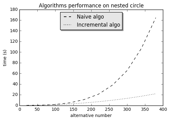
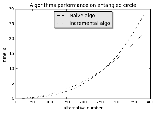
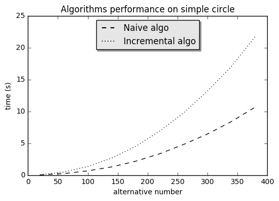
Figure 12: Performances on different preference structures

We observe that the incremental algorithm outperforms the naive algorithm when the structures contain a great number of nested circles. However, for the structures with little nested circles but many indifference relations, the naive algorithm performs better. So the selection of Condorcet Paradox avoidance algorithm should be adapted to the structure of the preferences.

VI Conclusion

In this paper, we introduced the problem of preference fusion with uncertainty degrees and proposed two belief-function-based strategies, one of which is applying the conjunctive rule on clusters, and which scales better with the number of sources. We also proposed a Condorcet Paradox avoidance method as well as an efficient DFS-based algorithm adapting to preference structure with nested circles. By comparing the temporal performance of the Condorcet Paradox avoidance algorithms on different types of preference structures, we noticed that the incremental algorithm is more efficient on nested structures while the naive algorithm is better on non-nested ones. Limited by our data sources, our experimental works were done on synthetic data. Furthermore, the algorithm for DAG construction can be applied in more general cases, other than those related to preference orders. In domains concerning directed graph with valued edges (e.g. telecommunication, social network analysis, etc.), algorithm 2 may find its usefulness.

There are still more works left to explore. Since our experiments are executed on synthetic data, we were not able to propose evaluation methods measuring quality fusion results. In our work, we proposed methods to guarantee the “transitivity” property, this property may help to reduce the number of “incomparable” alternative pairs. Besides, in the Condorcet Paradox avoidance process, as the preference structure is altered so an information entropy measuring method is supposed to be proposed. Lastly, in real world, alternatives are often represented in multi-criteria forms. Conventional multi-critera aggregation methods (e.g. AHP method[25], PROMETHEE method[26] and ELECTRE method[27]) have been proved to be efficient. By combining these methods with belief-function theory, new aggregation methods for multi-criteria alternatives under uncertainty may be proposed as future work.

References

- [1] M. Lacroix and P. Lavency, “Preferences: Putting more knowledge into queries,” Very Large Data Bases, p. 225, 1987.
- [2] L. Xiang, Q. Yuan, S. Zhao, L. Chen, X. Zhang, Q. Yang, and J. Sun, “Temporal recommendation on graphs via long- and short-term preference fusion,” in Proceedings of the 16th ACM SIGKDD International Conference on Knowledge Discovery and Data Mining, ser. KDD ’10. New York, NY, USA: ACM, 2010, pp. 723–732.
- [3] J. I. Marden, Analyzing and modeling rank data. CRC Press, 1995, vol. 64.
- [4] J.-A.-N. de Caritat marquis de Condorcet, Essai sur l’application de l’analyse à la probabilité des décisions rendues à la pluralité des voix. De l’Imprimerie royale, 1785.
- [5] F. Elarbi, T. Bouadi, A. Martin, and B. Ben Yaghlane, “Preference fusion for community detection in social networks,” in 24ème Conférence sur la Logique Floue et ses Applications, ser. 24ème Conférence sur la Logique Floue et ses Applications, Poitiers, France, Nov. 2015.
- [6] M. Öztürké, A. Tsoukiàs, and P. Vincke, Preference Modelling. New York, NY: Springer New York, 2005, pp. 27–59.
- [7] M. P. Wellman and J. Doyle, “Preferential semantics for goals,” in In Proceedings of the National Conference on Artificial Intelligence, 1991, pp. 698–703.
- [8] K. J. Arrow, “Rational choice functions and orderings,” Economica, vol. 26, no. 102, pp. 121–127, 1959.
- [9] G. Cox, Making Votes Count: Strategic Coordination in the World’s Electoral Systems, ser. Political Economy of Instituti. Cambridge University Press, 1997.
- [10] D. Dubois and H. Prade, “Representation and combination of uncertainty with belief functions and possibility measures,” Computational Intelligence, vol. 4, no. 3, pp. 244–264, 1988.
- [11] T. Denœux and M.-H. Masson, “Evidential reasoning in large partially ordered sets,” Annals of Operations Research, vol. 195, no. 1, pp. 135–161, 2012.
- [12] J. Schubert, “Partial ranking by incomplete pairwise comparisons using preference subsets,” pp. 190–198, 2014.
- [13] M.-H. Masson, S. Destercke, and T. Denoeux, “Modelling and predicting partial orders from pairwise belief functions,” Soft Computing, vol. 20, no. 3, pp. 939–950, 2016.
- [14] H. Nurmi, “Resolving group choice paradoxes using probabilistic and fuzzy concepts,” Group Decision and Negotiation, vol. 10, no. 2, pp. 177–199, 2001.
- [15] G. Shafer, A Mathematical Theory of Evidence. Princeton: Princeton University Press, 1976.
- [16] R. Tarjan, “Depth first search and linear graph algorithms,” SIAM JOURNAL ON COMPUTING, vol. 1, no. 2, 1972.
- [17] A.-L. Jousselme, D. Grenier, and Éloi Bossé, “A new distance between two bodies of evidence,” Information Fusion, vol. 2, no. 2, pp. 91 – 101, 2001.
- [18] N. D. Belnap, A Useful Four-Valued Logic. Dordrecht: Springer Netherlands, 1977, pp. 5–37.
- [19] A. P. Dempster, “Upper and lower probabilities induced by a multivalued mapping,” Ann. Math. Statist., vol. 38, no. 2, pp. 325–339, 04 1967.
- [20] P. Smets, “The combination of evidence in the transferable belief model,” IEEE Trans. Pattern Anal. Mach. Intell., vol. 12, no. 5, pp. 447–458, May 1990.
- [21] T. Denoeux, “The cautious rule of combination for belief functions and some extensions,” in 2006 9th International Conference on Information Fusion, July 2006, pp. 1–8.
- [22] P. Smets, Constructing the Pignistic Probability Function in a Context of Uncertainty, ser. UAI ’89. Amsterdam, The Netherlands: North-Holland Publishing Co., 1990, pp. 29–40.
- [23] A. Essaid, A. Martin, G. Smits, and B. Ben Yaghlane, “A Distance-Based Decision in the Credal Level,” in International Conference on Artificial Intelligence and Symbolic Computation (AISC 2014), Sevilla, Spain, Dec. 2014, pp. 147 – 156. [Online]. Available: https://hal.archives-ouvertes.fr/hal-01110349
- [24] A. Martin, A. L. Jousselme, and C. Osswald, “Conflict measure for the discounting operation on belief functions,” in 2008 11th International Conference on Information Fusion, June 2008, pp. 1–8.
- [25] T. L. Saaty, “Decision making with the analytic hierarchy process,” International journal of services sciences, vol. 1, no. 1, pp. 83–98, 2008.
- [26] J.-P. Brans and P. Vincke, “Note—a preference ranking organisation method: (the promethee method for multiple criteria decision-making),” Management science, vol. 31, no. 6, pp. 647–656, 1985.
- [27] B. Roy, “The outranking approach and the foundations of electre methods,” Theory and decision, vol. 31, no. 1, pp. 49–73, 1991.