Self-trapping self-repelling random walks

Abstract

Although the title seems self-contradictory, it does not contain a misprint. The model we study is a seemingly minor modification of the “true self-avoiding walk” (TSAW) model of Amit, Parisi, and Peliti in two dimensions. The walks in it are self-repelling up to a characteristic time $T^{*}$ (which depends on various parameters), but spontaneously (i.e., without changing any control parameter) become self-trapping after that. For free walks, $T^{*}$ is astronomically large, but on finite lattices the transition is easily observable. In the self-trapped regime, walks are subdiffusive and intermittent, spending longer and longer times in small areas until they escape and move rapidly to a new area. In spite of this, these walks are extremely efficient in covering finite lattices, as measured by average cover times.

Random walks are ubiquitous in nature, in science, and in technology. Be it the thermal motion of gas molecules Einstein , the evolution of financial indices Bachelier ; Bouchaud-Potters , the foraging of an animal Benichou , the Monte Carlo code of a scientist working in statistical physics Barkema , the shape of a randomly coiled polymer in a good solvent deGennes , or the carrying of a message in a random ad hoc network Avin : They are all more or less described by random walks, and thus random walks have been among the most studied objects in mathematical statistics Spitzer . But in most of these problems they only represent a first crude approximation. In a gas or liquid, there is usually also convection. Financial time series show heavy tailed distributions Bouchaud-Potters . And animal walks are not entirely random but also guided by the availability of food, and are often characterized by alternating periods of very slow and fast motion, what is often modelled as Levy flights levy . One of the most common deviations from perfect randomness is that random walks often have memory.

Maybe the best studied model of walks with memory are self-avoiding walks (SAWs) Madras , which describe the statistics of very long chain molecules, and where the “memory” takes care of the fact that in a growing polymer, a new monomer cannot be placed onto a site that is occupied already. This modification implies that in less than 4 dimensions of space the characteristic size of a polymer made of $N$ monomers increases faster than $\sim N^{1/2}$. More precisely, the increase follows, for $d<4$, a power law $R\sim N^{\nu}$ with $\nu>1/2$, while $R/N^{1/2}\sim(\ln N)^{\alpha}$ with $\alpha=1/4$ Clisby at the upper critical dimension $d=4$.

As pointed out by Amit et al. Amit , while SAWs are indeed self-avoiding as geometrical objects, they are as dynamical walks not self-avoiding but self-killing: When a walker tries to step on a site where she had already been, she is just killed. In what they called “true self-avoiding walks” (TSAWs), the walker instead tries to avoid in a short-sighted way to step on her own traces. Technically, this is implemented on a lattice by a walk where at each time step a unit of debris is dropped onto the site where the walker stands. As time goes on, a hilly landscape is formed where the height $h_{i}$ at site $i$ is just the amount of debris. The self-avoidance bias is then given by probabilities $p_{j}\propto e^{-\beta h_{j}}$ to step onto neighboring sites $j$, where $\beta$ plays the role of an inverse temperature. The self-avoidance is negligible for large temperature, while it is strongest for $\beta=\infty$. But even then its effect is much milder than in the original SAW model. No walker is killed, but they just try to turn away gently. In the mathematical literature, such walks are often called “self-repelling”.

In Amit it was shown that the upper critical dimension for TSAWs is not $d=4$ but $d=2$. Thus they show trivial scaling for $d>2$, while they are swollen, $R\sim N^{\nu}$ with $\nu>1/2$, for $d=1$. For $d=2$ there should be again logarithmic corrections, but the exponent in the ansatz $R/N^{1/2}\sim(\ln N)^{\alpha}$ is not known, in spite of considerable efforts Amit ; Obukhov ; Derkachov . A first attempt to obtain $\alpha$ was made in Amit , where an effective field theory was proposed in which the bias of the walk was – in a coarse-grained picture amenable to renormalization group (RG) ideas – coupled to the average local slope of $h_{i}$. It was neglected that the walker is not only influenced by the gradient of the landscape, but also by its roughness. As shown by Obukhov and Peliti Obukhov , this is not justified. It is well known that random walkers in rough landscapes are hindered by obstacles Bouchaud , so roughness tends to make them move more slowly. The RG scheme proposed in Obukhov was later criticized by Derkachov , who pointed out that one has in general to consider also higher order couplings (beyond slope and roughness), which makes the problem non-renormalizable. In SM we argue that $\alpha=1/2$.

Apart from these formal problems, the scheme proposed in Obukhov is also sick for a very basic reason. In an RG treatment of TSAWs, one has to consider not only the RG flow, but also the flow of time. Indeed, TSAWs are not stationary, and they are not even time reversal invariant SM . As the landscape grows, its effect on the walker becomes stronger and stronger.

To see this more quantitatively, let us consider TSAWs on a large but finite lattice of size $L\times L$. For convenience we take a square lattice with periodic (or, for easier coding, helical; the difference between them is negligible for the lattice sizes considered here) boundary conditions. The walker starts on a flat landscape $h_{i}=0$. If there were no self-repulsion (i.e. $\beta=0$), the lattice would be covered after a time $T_{\rm cover}\sim(4/\pi)L^{2}(\ln L)^{2}$ Dembo ; Grass-cover . After that, the average height still grows linearly with time, but its roughness also grows without limits Freund . The variance of the height profile,

$$\sigma(T)=L^{-2}\sum_{i}h_{i}^{2}-T^{2},$$ (1)

increases proportionally to $T$, and Freund

$$\sigma(T)/T=\frac{4}{\pi}\ln L+{\cal O}(1)\quad{\rm for}\;\;\;L\to\infty.$$ (2)

For non-zero $\beta$, in contrast, it was conjectured Avin that

$$T_{\rm cover}\sim a_{T}(\beta)L^{2}\ln L.$$ (3)

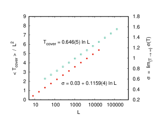
Figure 1: (color online) Log-linear plots of statistics of TSAWs with $\beta=\infty$ on square lattices of size $L\times L$ with helical boundary conditions. The upper curve (open squares and left-hand y-axis) shows the average cover times, divided by $L^{2}$. The lower curve (filled squares and right-hand y-axis) shows the asymptotic height variances of the debris field. In both cases, error bars are much smaller than symbol sizes.

For $\beta=\infty$ this is indeed shown in Fig. 1, but completely analogous results were obtained also for finite $\beta$. The prefactor $a_{T}(\beta)$ diverges of course for $\beta\to 0$.

For the height variance for $T\gg T_{\rm cover}$, the effect of self-repulsion is even stronger. This time the variance stays finite for $T\to\infty$, with Freund

$$\sigma(T)\sim a_{\sigma}(\beta)\ln L,$$ (4)

see also Fig. 1 for $\beta=\infty$. Again the prefactor $a_{\sigma}(\beta)$ diverges as $\beta\to 0$. From plots analogous to Fig. 1 (but for other values of $\beta$) we obtain

$$a_{\sigma}(\beta)\simeq 0.317(4)/\beta$$ (5)

for $\beta\to 0$.

In the RG treatment in Obukhov ; Derkachov it was assumed that one can start perturbatively around the point where both coupling constants (that for the slope and that for the roughness) are small. But as we have just seen, when the coupling to the slope is small, the roughness increases for late times beyond any limit. Thus a perturbative treatment in the combined effects of roughness and slope becomes impossible.

In order to avoid this problem, one can change the model so that the landscape becomes less rough. One possibility would be to let the debris diffuse. This could be presumably efficient, but it is rather awkward (and slow, from a numerical point of view) to implement – and it is very likely that it will lead to problems similar to those discussed below. Much easier seems the following change: Instead of dropping all debris onto the site of the walker, only a fraction $1-\epsilon$ is dropped there. The rest is distributed uniformly among all of its neighbors.

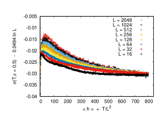
Figure 2: (color online) Plot of $\sigma(T)-a_{\sigma}(\beta=\infty,\epsilon)\ln L$ against the average debris height $\langle h\rangle$, for $\epsilon=1/2$. According to Eq. (4), these curves should all approach the same horizontal line for $T\to\infty$. The fact that they do this very slowly and in a non-monotonic way seems to be a peculiarity of the $\beta=\infty$ limit on the square lattice. It is neither seen for finite $\beta$ nor on the triangular lattice.

As seen from Fig. 2 for for $\beta=\infty$, this seems indeed to work – at least on the square lattice and for $\epsilon=\epsilon_{c}=1/2$. The variance increases still roughly according to Eq. (4), but the prefactor – called now $a_{\sigma}(\beta,\epsilon)$ – is $\lesssim 0.05$. Indeed, Fig. 2 does not show $a_{\sigma}(\beta,\epsilon)$ or $\sigma(T)$, but rather $\sigma(T)-a_{\sigma}(\beta=\infty,\epsilon)\ln L$. For reasons that are not fully understood, $\sigma(T)$ does not increase monotonically. This anomaly seems to be related to the fact that walks have strongly reduced randomness for $\beta=\infty$. It is even enhanced for $\epsilon<\epsilon_{c}$ SM . For finite $\beta$ this anomaly is absent, and the asymptotic value of $\sigma(T)$ is reached monotonically. The latter is true also for the triangular lattice (with $\epsilon_{c}=2/3$), and if debris on the square lattice is dropped not only onto the 4 nearest neighbors, but also (with the same amounts) onto the 4 next-nearest neighbors. In the last case we also found $\epsilon_{c}=2/3$ SM .

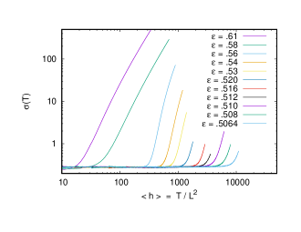
Figure 3: (color online) Log-log plot of $\sigma(T)$ against the average debris height $\langle h\rangle$, for square lattices with $L=512$. Each curve corresponds to a different value of $\epsilon$. They are roughly horizontal up to a characteristic debris height $h^{*}$ that increases roughly as an inverse power of $\epsilon=1/2$, but deviations from such a power law are much larger than statistical errors.

For $\epsilon>\epsilon_{c}$ things change, however, completely. As seen in Fig. 3, $\sigma(T)$ first approaches rapidly a constant, but finally increases beyond limit as $T\to\infty$. The data in Fig. 3 are for the square lattice with $L=512$ and $\beta=\infty$, but similar results were seen also in all other cases. In particular, nearly identical plots are obtained for $L=256$ and $L=1024$, the only difference being tiny shifts compensating the height differences of the curves before they start to rise. This means that the rise of $\sigma(T)$ starts at a fixed debris height, not at a fixed time. This implies also that the same rise should also be seen on an infinite lattice, because debris height increases also there with time. Since this increase is only logarithmic on an infinite lattice, the transition happens there at astronomically large times, making it de facto unobservable.

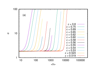
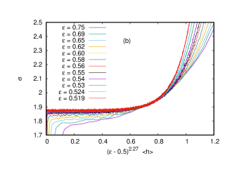
Figure 4: (color online) (a) Plot of $\sigma(T)$ against $\langle h\rangle$, but for $\beta=1.0$. (b) Same data, but plotted against $(\epsilon-1/2)^{2.27}\langle h\rangle$.

Roughly, the characteristic densities $h^{*}$ in Fig.3 (at which roughness starts to increase) scale as $h^{*}\sim(\epsilon-1/2)^{-2}$, but deviations from this are huge. The reason is most likely the same as that for the non-monotonicity in Fig. 2. Much more regular behavior is found for finite $\beta$ and on the triangular lattice. Results for $\beta=1$ on the square lattice are shown in Fig. 4. In panel (a) we show $\sigma$ versus $\langle h\rangle$, while the data are plotted against $(\epsilon-1/2)^{2.27}\langle h\rangle$ in panel (b). The latter suggests strongly that (i) $\epsilon_{c}=1/2$ is exact; (ii) The characteristic height scales as $h^{*}=c/(\epsilon-1/2)^{\gamma}$ with $c=0.80(5)$ and $\gamma=2.27(2)$; and (iii) At $h=h^{*}$, the rise of $\sigma$ against $(\epsilon-1/2)^{\gamma}h$ becomes infinitely steep for $\epsilon\to 1/2$.

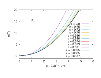
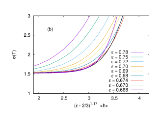
Figure 5: (color online) Plots of $\sigma(T)$ against $(\epsilon-1/2)^{\gamma}\langle h\rangle$, for triangular lattices. Panel (a) is for $\beta=\infty$ and $\gamma=1.0$, while (b) is for $\beta=1.0$ and $\gamma=1.17$.

Basically the same results were found also for $\beta=0.2$ and $\beta=5.0$. In particular, also there $\epsilon_{c}$ seems to be exactly $1/2$ and the same scaling seems to hold for $h^{*}$, with $c=4.3(5)$ for $\beta=0.2$ and $c=0.26(3)$ for $\beta=5.0$. The values for the exponent $\gamma$ are $2.24(3)$ and $2.26(3)$.

This suggests that $\gamma$ is universal, but this is shattered by the results for the triangular lattice. There, $\epsilon_{c}=2/3$ (again for all values of $\beta$), but plots analogous to Fig. 4b for $\beta=\infty$ (see Fig. 5a) and $\beta=1$ (see Fig. 5b) indicate that $\gamma\approx 1$ in both cases More precisely, for $\beta=\infty$ we obtained $\gamma=1.00(2)$, while $\gamma\leq 1.17$ for $\beta=1$ (a more precise estimate for the latter is prevented by large corrections to scaling). Finally, we simulated also walks on the square lattice where the four next-nearest neighbors received the same amount of debris as the four nearest neighbors. The data SM gave again $\epsilon_{c}=2/3$ for all $\beta$ and $\gamma=1.00(1)$ for $\beta=\infty$, while the estimate $\gamma\leq 1.15$ for $\beta=1$ is again affected by large corrections to scaling. In summary, it seems that there are two distinct universality classes, one with $\gamma\approx 1$, and the other with $\gamma\approx 2$. Within each class, there are still minor but statistically significant differences. The origin of this is not clear.

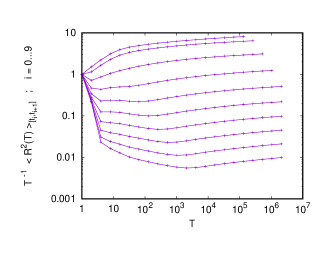
Figure 6: (color online) Squared average end-to-end distances (divided by $T$) of the $T$ last steps of walks with total length $t\in[t_{i},t_{i+1}],\;\;0\leq i<10,\;t_{0}=0,\;t_{i+1}=2t_{i}+4L^{2}$. The top curve is for $i=0$, the bottom one for $i=9$. Parameters are $L=16384$, $\beta=\infty$ and $\epsilon=0.7$.

For $h>h^{*}$, walks are subdiffusive and get more and more so as $h$ increases further. Let us define the average squared end-to-end distance of the last $T$ steps of a walk of total length $t$, averaged over $t\in[t_{a},t_{b}]$, as $\langle R^{2}(T)\rangle_{[t_{a},t_{b}]}$. In Fig. 6 are plotted $T^{-1}\langle R^{2}(T)\rangle_{[t_{i},t_{i+1}]}$ for $t_{i+1}=2t_{i}+4L^{2}$, with $t_{0}=0,0\leq i<10$, and $L=16384$. We see that the walks are stretched for all $T$ for $i=0,1$, and remain stretched for large $T$ even when $i=2$ or 3. But for larger $i$ we see $R^{2}<T$, mainly because the walks are strongly compressed for very small $T$.

Thus, most of the time the walks are confined to narrow regions for short intervals whose length increases with $i$, while the evolution on larger time scales is characterized by escape from these regions. Obviously, a typical walk stays for some time trapped in a region where $h$ was originally lower than average. As time goes on, it fills up the debris in this region, but it also builds a wall around it. When finally $h$ is so large that the walk escapes, it has built such a high wall that it gets trapped even longer in a neighboring region, etc. This scenario is supported by the entropy of the walks, which is just equal to the entropy provided by the random number generator. Entropies decrease fast (roughly exponentially) with $\langle h\rangle$ SM , implying that for large times the walk is hardly random at all.

We have seen that self-repelling walks become self-trapping when the debris height increases above a critical height, if sufficiently much of the debris is placed on neighboring sites. The critical height depends on this amount and on the type of lattice, but it is independent of the size of the lattice. Since the average debris height increases also for infinite lattices, this transition should be also seen there. Since this increase is however very slow ($\sim\ln T$), the self-trapping transition on infinite lattices should be seen only at extremely large times, much larger than what is reachable with present-day computers. Therefore, also lattice covering times should not – at presently reachable values of $L$ – be affected by self-trapping, unless $\epsilon$ is extremely large. For the square lattice with $\epsilon=0.8$, e.g., we found that Eq. (3) holds for $\beta=\infty$ with $\sigma_{T}(\infty)=0.024(2)$. Thus walks with large $\epsilon$ should be optimal for disseminating/collecting information on large systems (notice that our results should also apply on geometric random graphs Avin ). Even faster could be walks where also next-nearest neighbors of visited sites are marked, but then the increased efficiency in terms of number of steps should be balanced against increased effort in marking these sites.

I am indebted to Gerhard Gompper, Dmitry Fedosov, and Sandipan Mohanty for most useful discussions.

References

- (1) A. Einstein, Annalen der Physik, 322, 549 (1905).
- (2) L. Bachelier, Théorie de la spéculation (Gauthier-Villars, Paris, 1900).
- (3) M.E.J. Newman and G.T. Barkema, Monte Carlo Methods in Statistical Physics (Oxford University Press, New York 1999).
- (4) P.G. de Gennes, Scaling Concepts in Polymer Physics (Cornell University Press, Ithaca N.Y. 1979).
- (5) O. Bénichou, C. Loverdo, M. Moreau, and R. Voituriez, Rev. Mod. Phys. 83, 81 (2011).
- (6) C. Avin and B. Krishnamachari, Computer Networks 52,44 (2008).
- (7) F. Spitzer, Principles of random walk (Springer, New York 2013).
- (8) J.-P. Bouchaud and M. Potters, Theory of financial risk and derivative pricing: from statistical physics to risk management, (Cambridge university press, 2003).
- (9) N.E. Humphries, H. Weimerskirch, N. Queiroz, E.J. Southall, and D.W. Sims, PNAS 109, 7169 (2012).
- (10) N. Madras, and G. Slade, The self-avoiding walk (Springer Science & Business Media, 2013).
- (11) N. Clisby, e-print arXiv:1703.10557 (2017).
- (12) D. Amit, G. Parisi, and L. Peliti, Phys. Rev. B 27, 1635 (1983).
- (13) S.P. Obukhov and L. Peliti, J. Phys. A: Math. Gen. 16, L147 (1983).
- (14) S.E. Derkachov, J. Honkonen, E. Karjalainen, and A.N. Vasil’ev, J. Phys. A: Math. Gen. 22, L385 (1989).
- (15) J.-P. Bouchaud and A. Georges, Physics reports 195, 127 (1990).
- (16) Supplemental material.
- (17) A. Dembo, Y. Peres, J. Rosen, and O. Zeitouni, Ann. Math. 160, 433 (2004).
- (18) P. Grassberger, e-print arXiv:1704.05039 (2017).
- (19) H. Freund and P. Grassberger, Physica A 192, 465 (1993).