Fast and accurate Bayesian model criticism and conflict diagnostics using R-INLA

Abstract

Bayesian hierarchical models are increasingly popular for realistic modelling and analysis of complex data. This trend is accompanied by the need for flexible, general and computationally efficient methods for model criticism and conflict detection. Usually, a Bayesian hierarchical model incorporates a grouping of the individual data points, as, for example, with individuals in repeated measurement data. In such cases, the following question arises: Are any of the groups “outliers,” or in conflict with the remaining groups? Existing general approaches aiming to answer such questions tend to be extremely computationally demanding when model fitting is based on Markov chain Monte Carlo. We show how group-level model criticism and conflict detection can be carried out quickly and accurately through integrated nested Laplace approximations (INLA). The new method is implemented as a part of the open-source R-INLA package for Bayesian computing (http://r-inla.org).
Keywords: Bayesian computing; Bayesian modelling; INLA; model criticism; model assessment; latent Gaussian models

1 Introduction

The Bayesian approach gives great flexibility for realistic modelling of complex data. However, any assumed model may be unreasonable in light of the observed data, and different parts of the data may be in conflict with each other. Therefore, there is an increasing need for flexible, general and computationally efficient methods for model criticism and conflict detection. Usually, a Bayesian hierarchical model incorporates a grouping of the individual data points. For example, in clinical trials, repeated measurements are grouped by patient; in disease mapping, cancer counts may be grouped by year or by geographical area. In such cases, the following question arises: Are any of the groups “outliers,” or in conflict with the remaining groups? Existing general approaches aiming to answer such questions tend to be extremely computationally demanding when model fitting is based on Markov chain Monte Carlo (MCMC). We show how group-level model criticism and conflict detection can be carried out quickly and accurately through integrated nested Laplace approximations (INLA). The new method is implemented as a part of the open-source R-INLA package for Bayesian computing (http://r-inla.org); see Section 3 for details about the implementation.

The method is based on so-called node-splitting (Marshall and Spiegelhalter,, 2007; Presanis et al.,, 2013), which has previously been used by one of the authors (Sauter and Held,, 2015) in network meta-analysis (Lumley,, 2002; Dias et al.,, 2010) to investigate whether direct evidence on treatment comparisons differs from the evidence obtained from indirect comparisons only. The assessment of possible network inconsistency by node-splitting implies that a network meta-analysis model is fitted repeatedly for every directly observed comparison of two treatments where also indirect evidence is available. For network meta-analysis, the INLA approach has been recently shown to provide a fast and reliable alternative to node-splitting based on MCMC (Sauter and Held,, 2015). This has inspired the work described here to develop general INLA routines for model criticism in Bayesian hierarchical models.

This paper is organized as follows. In Section 2, we describe the methodology based on the latent Gaussian modelling framework outlined in Section 2.1. Specifically, Section 2.2 describes general approaches to model criticism in Bayesian hierarchical models, while Section 2.3 outlines our proposed method for routine analysis within INLA. Section 3 discusses the implementation in the R-INLA package. We provide two applications in Section 4 and close with some discussion in Section 5.

2 Methodology

2.1 Latent Gaussian models and INLA

The class of latent Gaussian models (LGMs) includes many Bayesian hierarchical models of interest. This model class is intended to provide a good trade-off between flexibility and computational efficiency: for models within the LGM class, we can bypass MCMC completely and obtain accurate deterministic approximations using INLA. The LGM/INLA framework was introduced in Rue et al., (2009); for an up-to-date review covering recent developments, see Rue et al., (2017).

We shall only give a very brief review of LGM/INLA here; for more details, see the aforementioned references, as well as Rue and Held, (2005) for more background on Gaussian Markov random fields, which form the computational backbone of the method. The basic idea of the LGM is to split into a hierarchy with three levels:

1. The (hyper)prior level, with the parameter vector $\boldsymbol{\theta}$. It is assumed that the dimension of $\boldsymbol{\theta}$ is not too large (less than 20; usually 2 to 5). Arbitrary priors (with restrictions only on smoothness / regularity conditions) can be specified independently for each element of $\boldsymbol{\theta}$ (and there is ongoing work on allowing for more general joint priors; see Simpson et al., (2017) for ideas in this direction). Also, it is possible to use the INLA-estimated posterior distribution of $\boldsymbol{\theta}$ as the prior for a new run of INLA; we shall use this feature here.

2. The latent level, where the latent field $\boldsymbol{x}$ is assumed to have a multivariate Gaussian distribution conditionally on the hyperparameters $\boldsymbol{\theta}$. The dimension of $\boldsymbol{x}$ may be very large, but conditional independence properties of $\boldsymbol{x}|\boldsymbol{\theta}$ typically implies that the precision matrix (inverse covariance matrix) in the multivariate Gaussian is sparse (i.e. $\boldsymbol{x}$ is a Gaussian Markov random field), allowing for a high level of computational efficiency using methods from sparse linear algebra.

3. The data level, where observations $\boldsymbol{y}$ are conditionally independent given the latent field $\boldsymbol{x}$. In principle, the INLA methodology allows for arbitrary data distributions (likelihood functions); a long list of likelihood functions (including normal, Poisson, binomial and negative binomial) are currently implemented in the R-INLA package.

It is assumed that the joint posterior of $(\boldsymbol{x},\boldsymbol{\theta})$ can be factorized as

$$\pi(\boldsymbol{x},\boldsymbol{\theta}|\boldsymbol{y})\propto\pi(\boldsymbol{\theta})\pi(\boldsymbol{x}|\boldsymbol{\theta})\prod_{i\in\mathcal{I}}\pi(y_{i}|x_{i},\boldsymbol{\theta})$$ (1)

where $\mathcal{I}$ is a subset of $\{1,2,\ldots,n\}$ and where $n$ is the dimension of the latent field $\boldsymbol{x}$.

In R-INLA, the model is defined in a format generalizing the well-known generalized linear/additive (mixed) models: for each $i$, the linear predictor $\eta_{i}$ is modelled using additive building blocks, for example as (Equation (2) of Rue et al., (2017)):

$$\eta_{i}=\mu+\sum_{j}\beta_{j}z_{ij}+\sum_{k}f_{k,j_{k}(i)}$$ (2)

where $\mu$ is an overall intercept, the $\beta_{j}$ are “fixed effects” of covariates $z_{ij}$, and the $f_{k}$ terms represent Gaussian process model components, which can be used for random effects models, spatial models, time-series models, measurement error models, spline models and so on. The wide variety of possible $f_{k}$ terms makes this set-up very general, and it covers most of the Bayesian hierarchical models used in practice today. As in the usual generalized linear model framework (McCullagh and Nelder,, 1989), the linear predictor $\eta_{i}$ is related to the mean of data point $y_{i}$ (or, more generally, the location parameter of the likelihood) through a known link function $g$. For example, in the Poisson likelihood with expected value $\lambda_{i}$, the log link function is used, and the linear predictor is $\eta_{i}=\log(\lambda_{i})$. Assuming a priori independent model components and a multivariate Gaussian prior on $(\mu,\boldsymbol{\beta})$, we can define the latent field as $\boldsymbol{x}=(\boldsymbol{\eta},\mu,\boldsymbol{\beta},\boldsymbol{f}_{1},\boldsymbol{f}_{2},\ldots)$, with a small number of hyperparameters $\boldsymbol{\theta}$ arising from the likelihood and model components. It follows that $\boldsymbol{x}$ has a multivariate Gaussian distribution conditionally on $\boldsymbol{\theta}$, so we are in the LGM class described earlier. For advice on how to set the priors on $\boldsymbol{\theta}$, see Simpson et al., (2017).

Why restrict to the LGM class? The reason is that quick, deterministic estimation of posterior distributions is possible for LGMs, using INLA. Here, we only give a brief sketch of how this works; for further details, see Rue et al., (2009) and Rue et al., (2017). Assume that the objects of interest are the marginal posterior distributions $\pi(x_{i}|\boldsymbol{y})$ and $\pi(\theta_{j}|\boldsymbol{y})$ of the latent field and hyperparameters, respectively. The full joint distribution is

$$\pi(\boldsymbol{x},\boldsymbol{\theta},\boldsymbol{y})=\pi(\boldsymbol{\theta})\pi(\boldsymbol{x}|\boldsymbol{\theta})\prod_{i\in\mathcal{I}}\pi(y_{i}|x_{i},\boldsymbol{\theta})$$

(cf. Equation (1) earlier). We begin by noting that a Gaussian approximation $\tilde{\pi}_{G}(\boldsymbol{x}|\boldsymbol{\theta},\boldsymbol{y})$ can be calculated relatively easily, by matching the mode and curvature of the mode of $\pi(\boldsymbol{x}|\boldsymbol{\theta},\boldsymbol{y})$. Then, the Laplace approximation (Tierney and Kadane,, 1986) of the posterior $\pi(\boldsymbol{\theta}|\boldsymbol{y})$ is given by

$$\tilde{\pi}(\boldsymbol{\theta}|\boldsymbol{y})\propto\left.\frac{\pi(\boldsymbol{x},\boldsymbol{\theta},\boldsymbol{y})}{\tilde{\pi}_{G}(\boldsymbol{x}|\boldsymbol{\theta},\boldsymbol{y})}\right|_{\boldsymbol{x}=\boldsymbol{\mu}(\boldsymbol{\theta)}},$$

where $\boldsymbol{\mu}(\boldsymbol{\theta})$ is the mean of the Gaussian approximation. Because the dimension of $\boldsymbol{\theta}$ is not too large, the desired marginal posteriors can then be calculated using numerical integration:

$$\tilde{\pi}(\theta_{j}|\boldsymbol{y}) = \int\tilde{\pi}(\boldsymbol{\theta}|\boldsymbol{y})\mathrm{d}\boldsymbol{\theta}_{-j},$$

$$\tilde{\pi}(x_{i}|\boldsymbol{y}) = \int\tilde{\pi}(x_{i}|\boldsymbol{\theta},\boldsymbol{y})\tilde{\pi}(\boldsymbol{\theta}|\boldsymbol{y})\mathrm{d}\boldsymbol{\theta},$$

where the approximation $\pi(x_{i}|\boldsymbol{\theta},\boldsymbol{y})$ is calculated using a skew normal density (Azzalini and Capitanio,, 1999). This approach is accurate enough for most purposes, but see Ferkingstad and Rue, (2015) for an improved approximation useful in particularly difficult cases.

The methodology is implemented in the open-source R-INLA R package; see http://r-inla.org for documentation, case studies etc. There are also a number of features allowing to move beyond the framework above (including the “linear combination” feature we will use later), see Martins et al., (2013).

2.2 Model criticism and node-splitting

Using INLA (or other Bayesian computational approaches), we can fit a wide range of possible models. With this flexibility comes the need to check that the model is adequate in light of the observed data. In the present paper, we will not discuss model comparison, except for pointing out that R-INLA already has implemented standard model comparison tools such as the deviance information criterion (Spiegelhalter et al.,, 2002) and then Watanabe-Akaike information criterion (Watanabe,, 2010; Vehtari et al.,, 2016). We shall only discuss model criticism, that is, investigating model adequacy without reference to any alternative model.

Popular approaches to Bayesian model criticism include posterior predictive $p$-values (Gelman et al.,, 1996) as well as cross-validatory predictive checks such as the conditional predictive ordinate (CPO) (Pettit,, 1990) and the cross-validated probability integral transform (PIT) (Dawid,, 1984). All of these measures are easily available from R-INLA (and can be well approximated without actually running a full cross-validation); see Held et al., (2010) for a review and practical guide. As noted by Held et al., (2010) (see also Bayarri and Castellanos, (2007)), posterior predictive $p$-values have the drawback of not being properly calibrated: they are not uniformly distributed, even if the data come from the assumed model, and are therefore difficult to interpret. The problem comes from “using the data twice,” as the same data are used both to fit and criticize the model. Because cross-validation avoids this pitfall, we recommend the use of cross-validatory measures such as CPO or PIT.

For illustration consider the following simple example. Suppose $y_{1},\ldots,y_{n}$ are independent realisations from a $\operatorname{N}(\mu,\sigma^{2})$ distribution with unknown $\mu$ and known $\sigma^{2}$. For simplicity suppose a flat prior is used for $\mu$. Then:

$$\mu\,|\,y_{-i} \sim \operatorname{N}(\bar{y}_{-i},\sigma^{2}/(n-1))$$ (3)

$$\mu\,|\,y_{i} \sim \operatorname{N}(y_{i},\sigma^{2})$$ (4)

so

$$y_{i}\,|\,y_{-i}=\int[y_{i}\,|\,\mu][\mu\,|\,y_{-i}]d\mu\sim\operatorname{N}(\bar{y}_{-i},\underbrace{\sigma^{2}\cdot n/(n-1)}_{=:\tilde{\sigma}^{2}})$$

and we obtain the PIT value

$$\mbox{PIT}_{i}=\Pr\{Y_{i}\leq y_{i}\,|\,y_{-i}\}=\Phi((y_{i}-\bar{y}_{-i})/\tilde{\sigma}).$$ (5)

If the model is true, then $(Y_{i}-\bar{Y}_{-i})/\tilde{\sigma}\sim\operatorname{N}(0,1)$ and therefore $\mbox{PIT}_{i}\sim\operatorname{U}(0,1)$.

Alternatively we could also consider the difference of (3) and (4)

$$\delta=\mu\,|\,y_{i}-\mu\,|\,y_{-i}\sim\operatorname{N}(\underbrace{\bar{y}_{-i}-{y}_{i}}_{\mu_{\delta}},\underbrace{\sigma^{2}+\sigma^{2}/(n-1)}_{=\tilde{\sigma}^{2}})$$

and compute with $\tilde{\delta}=(\delta-\mu_{\delta})/\tilde{\sigma}\sim\operatorname{N}(0,1)$ the tail probability

$$\Pr\{\delta\leq 0\}=\Pr\{\tilde{\delta}\leq-\mu_{\delta}/\tilde{\sigma}\}=\Phi((y_{i}-\bar{y}_{-i})/\tilde{\sigma}),$$ (6)

which is the same as (5). This shows that in this simple model, the PIT approach based on observables ($y_{i}$) is equivalent to the latent approach based on the distribution of $\delta$.

Both (5) and (6) are one-sided tail probabilities. A two-sided version of (6) can easily be obtained by considering $\tilde{\delta}^{2}\sim\chi^{2}(1)$ so the two-sided tail probability is

$$p = 2\min\{\Pr\{\tilde{\delta}\leq-\mu_{\delta}/\tilde{\sigma}\},1-\Pr\{\tilde{\delta}\leq-\mu_{\delta}/\tilde{\sigma}\}\}$$

$$= 1-\Pr\{{\tilde{\delta}^{2}}\leq\mu_{\delta}^{2}/\tilde{\sigma}^{2}\}$$

$$= \Pr\{{\tilde{\delta}^{2}}\geq\mu_{\delta}^{2}/\tilde{\sigma}^{2}\}.$$

A limitation of all the measures discussed above is that they only operate on the data level and on a point-by-point basis: each data point $y_{i}$ is compared with the model fit either from the remaining data points $\boldsymbol{y}_{-i}$ (for the cross-validatory measures) or from the full data $\boldsymbol{y}$ (for posterior predictive measures). However, often there is an interest in queries of model adequacy where we look more generally into whether any sources of evidence conflict with the assumed model. As a simple example, consider a medical study with repeated measures: Each patient $j=1,\ldots,J$ has some measurement taken at time points $t=1,\ldots,T$, giving rise to data points $z_{jt}$ (corresponding to the “$y_{i}$” in the general notation). For this example, it seems natural to consider each patient as a “source of evidence,” and we may wish to consider model adequacy for each patient, for example, asking whether any particular patient is an “outlier” according to the model. However, the methods above do not provide any easy way of answering such questions, as they are limited to looking directly at the data points $z_{jt}$. To answer questions such as “is patient NN an outlier,” we need to approach the model criticism task somewhat differently: rather than looking directly at data points $y_{i}$, we need to lift the model criticism up to the latent level of the model.

In our view, the most promising approach aiming to achieve this goal is the cross-validatory method known as node-splitting, proposed by Marshall and Spiegelhalter, (2007) and extended by Presanis et al., (2013). The word “node” refers to a vertex (node) in a directed acyclic graph (DAG) representing the model, but for our purposes here, it is not necessary to consider the DAG for the model (“parameter-splitting” would perhaps be a better name for the method). To explain node-splitting, we begin by considering some grouping of the data. For example, in the repeated measures case described above, the data $\boldsymbol{y}$ can be grouped by patient $j=1,\ldots,J$, such that $\boldsymbol{y}_{j}=(y_{j1},\ldots,y_{jT})^{\prime}$. In general, we let $\boldsymbol{y}_{j}$ denote the data for group $j$, while $\boldsymbol{y}_{-j}$ are the data for all remaining groups $1,\ldots,j-1,j+1,\ldots,J$. Further, consider a (possibly multivariate) group-level parameter $\boldsymbol{\gamma}_{j}$ in the model. (For the moment, $\boldsymbol{\gamma}_{j}$ may be any parameter of the model, but we shall make a particular choice of $\boldsymbol{\gamma}_{j}$ in the next section.) The basic idea behind node-splitting is to consider both the “within-group” posterior $\pi(\boldsymbol{\gamma}_{j}|\boldsymbol{y}_{j})$ and the “between-group” posterior $\pi(\boldsymbol{\gamma}_{j}|\boldsymbol{y}_{-j})$ for each group $j$, in effect splitting the evidence informing the “node” $\boldsymbol{\gamma}_{j}$ between

1. the evidence provided by group $j$, and

2. the evidence provided by the other groups

Now, the intuition is that if group $j$ is consistent with the other groups, then $\pi(\boldsymbol{\gamma}_{j}|\boldsymbol{y}_{j})$ and $\pi(\boldsymbol{\gamma}_{j}|\boldsymbol{y}_{-j})$ should not differ too much. A test for consistency between the groups can be constructed by considering the difference

$$\boldsymbol{\delta}_{j}=\boldsymbol{\gamma}_{j}^{(-j)}-\boldsymbol{\gamma}_{j}^{(j)},$$ (7)

where $\boldsymbol{\gamma}_{j}^{(-j)}\sim\pi(\boldsymbol{\gamma}_{j}|\boldsymbol{y}_{-j})$ and $\boldsymbol{\gamma}_{j}^{(j)}\sim\pi(\boldsymbol{\gamma}_{j}|\boldsymbol{y}_{j})$, and testing $H_{0}$: $\boldsymbol{\delta}_{j}=\boldsymbol{0}$ for each group $j$. We shall explain a specific way to construct such a test in Section 2.3, but see Presanis et al., (2013) for further details and alternative approaches to performing the test for conflict detection.

2.3 General group-wise node-splitting using R-INLA

In principle, the node-splitting procedure described in Section 2.2 can be implemented using sampling-based (i.e. MCMC-based) methods; see, for example, Marshall and Spiegelhalter, (2007) and Presanis et al., (2013). However, there are a number of problems with existing approaches, and these concerns are both of a theoretical and practical nature:

1. In our view, the most important problem is computational: running the group-wise node-splitting procedure using MCMC becomes very computationally expensive for all but the smallest models and data sets.

2. Related to the computational problem above is the implementational issue: even though there exist well-developed computational engines for MCMC (such as OpenBUGS (Lunn et al.,, 2009), JAGS (Plummer,, 2016) and STAN (Carpenter et al.,, 2017)), there is not to our knowledge any available software that can add the node-split group-wise model criticism functionality to an existing model. Thus, for a given model, actually implementing the node-split requires a non-trivial coding task, even if the model itself is already implemented and running in OpenBUGS, JAGS or STAN.

3. There is also an unsolved problem concerning what should be done with shared parameters. For example, if the node-split parameter corresponds to independent random effects $\gamma_{j}\sim N(0,\sigma^{2})$, the variance $\sigma^{2}$ is then shared between the different $\gamma_{j}$. The existence of the shared parameter $\sigma^{2}$ implies that $\boldsymbol{\gamma}_{j}^{(-j)}$ and $\boldsymbol{\gamma}_{j}^{(j)}$ from Equation (7) are not independent, and there are also concerns about estimating $\sigma^{2}$ based on group $j$ alone, since the number of data points within each point may be small. Marshall and Spiegelhalter, (2007) and Presanis et al., (2013) suggest to treat shared parameters as “nuisance parameters”, by placing a “cut” in DAG, preventing information flow from group $j$ to the shared parameter. However, it turns out that implementing the “cut” concept within MCMC algorithms is a difficult matter. Discussion of practical and conceptual issues connected to the “cut” concept has mainly been taking place on blogs and mailing lists rather than in traditional refereed journals, but a thorough review is nevertheless provided by Plummer, (2015), who is the author of the JAGS software. Plummer, (2015) shows that the “cut” functionality (recommended by Presanis et al., (2013)) implemented in the OpenBUGS software “does not converge to a well-defined limiting distribution,” i.e. it does not work. We are not aware of any correct general MCMC implementation.

Our approach using INLA solves all of the issues above. The first issue (computation intractability) is dealt with simply because INLA is orders of magnitude faster than MCMC, making cross-validation-based approaches manageable. The second issue is also dealt with: We provide a general implementation that only needs the model specification and an index specifying the grouping, so implementation of the extra step of running the node-split model checking (given that the user already has a working INLA model) is a trivial task. We also provide an elegant solution of the third issue of “shared parameters”/”cuts,” implementing the “cut” using an approach equivalent to what Plummer, (2015) calls “multiple imputation.”

The key to solving the second issue, that is, making a general, user-friendly implementation, is to make one specific choice of parameter for the node-split: the linear predictor $\boldsymbol{\eta}$. Intuitively, this is what the model “predicts” on the latent level, so it seems to make sense to use it for a measure of predictive accuracy. The main advantage of $\boldsymbol{\eta}$ is that it will always exist for any model in INLA, making it possible to provide a general implementation. Thus, the node split is implemented by providing a grouping $j=1,\ldots,J$. Formally, the grouping is a partition of the index set of the observed data $\boldsymbol{y}$. For each group $j$, we collect the corresponding elements in $\boldsymbol{\eta}$ (i.e. corresponding to data $\boldsymbol{y}_{j}$ contained in group $j$) into the vector $\boldsymbol{\eta}_{j}$. The node-splitting procedure sketched at the end of Section 2.2 then follows through, simply by replacing the general parameter $\boldsymbol{\gamma}_{j}$ with $\boldsymbol{\eta}_{j}$, and considering the difference

$$\boldsymbol{\delta}_{j}=\boldsymbol{\eta}_{j}^{(-j)}-\boldsymbol{\eta}_{j}^{(j)},$$ (8)

where $\boldsymbol{\eta}_{j}^{(-j)}\sim\pi(\boldsymbol{\eta}_{j}|\boldsymbol{y}_{-j})$ and $\boldsymbol{\eta}_{j}^{(j)}\sim\pi(\boldsymbol{\eta}_{j}|\boldsymbol{y}_{j})$. We then wish to test $H_{0}$: $\boldsymbol{\delta}_{j}=\boldsymbol{0}$ for each group $j$. It is often reasonable to assume multivariate normality of the posterior $\pi(\boldsymbol{\delta}_{j}|\boldsymbol{y})$ (see the discussion in Section 5 for alternative approaches if we are not willing to assume approximate posterior normality). If we denote the posterior expectation of $\boldsymbol{\delta}_{j}$ by $\boldsymbol{\mu}(\boldsymbol{\delta}_{j})$ and the posterior covariance by $\boldsymbol{\Sigma}(\boldsymbol{\delta}_{j})$, the standardized discrepancy measure

$$\Delta_{j}=\boldsymbol{\mu}(\boldsymbol{\delta}_{j})^{\top}\boldsymbol{\Sigma}(\boldsymbol{\delta}_{j})^{-}\boldsymbol{\mu}(\boldsymbol{\delta}_{j})$$

(where $\boldsymbol{\Sigma}(\boldsymbol{\delta}_{j})^{-}$ is then a Moore-Penrose generalized inverse of $\boldsymbol{\Sigma}(\boldsymbol{\delta}_{j})$) has a $\chi^{2}$-distribution with $r=\text{Rank}(\boldsymbol{\Sigma}(\boldsymbol{\delta}_{j}))$ degrees of freedom under $H_{0}$. The discrepancy measure above is a generalization of the measure suggested by Gåsemyr and Natvig, (2009) and Presanis et al., (2013, option (i) in Section 3.2.3 on page 384), extended to the case where $\boldsymbol{\Sigma}(\boldsymbol{\delta}_{j})$ does not necessarily have full rank (typically, $\boldsymbol{\Sigma}(\boldsymbol{\delta}_{j})$ will have less than full rank).

For each group $j$, an estimate of $\Delta_{j}$ is calculated by using two INLA runs: first, a “between-group” run is performed by removing (set to NA) the data in group $j$, providing an estimate for $\pi(\boldsymbol{\eta}_{j}|\boldsymbol{y}_{-j})$. Second, a “within-group” run is performed using only the data in group $j$, thus providing an estimated $\pi(\boldsymbol{\eta}_{j}|\boldsymbol{y}_{j})$. The “shared parameter”/”cut” problem described in item 3 above is dealt with by using an INLA feature allowing us to use the estimated posterior of the hyperparameters $\boldsymbol{\theta}$ from an INLA run as the prior for a subsequent INLA run: we can then simply use the posterior of the hyperparameters from the “between-group” run as the prior for the “within-group” run. This corresponds exactly to Plummer,’s (2015) recommended “multiple imputation” solution of the “cut” issue.

Using the linear combination feature of INLA (see Section 4.4 of Martins et al., (2013)), estimates of the posterior means and covariance matrices from both $\pi(\boldsymbol{\eta}_{j}|\boldsymbol{y}_{-j})$ and $\pi(\boldsymbol{\eta}_{j}|\boldsymbol{y}_{j})$ can be calculated quickly, and we can calculate the observed discrepancy

$$\widehat{\Delta}_{j}=\widehat{\boldsymbol{\mu}}(\boldsymbol{\delta}_{j})^{\top}\widehat{\boldsymbol{\Sigma}}(\boldsymbol{\delta}_{j})^{-}\widehat{\boldsymbol{\mu}}(\boldsymbol{\delta}_{j})$$

where

$$\widehat{\boldsymbol{\mu}}(\boldsymbol{\delta}_{j}) = \widehat{\boldsymbol{\mu}}(\boldsymbol{\eta}_{j}^{(-j)})-\widehat{\boldsymbol{\mu}}(\boldsymbol{\eta}_{j}^{(j)}),\ \text{and}$$

$$\widehat{\boldsymbol{\Sigma}}(\boldsymbol{\delta}_{j}) = \widehat{\boldsymbol{\Sigma}}(\boldsymbol{\eta}_{j}^{(-j)})+\widehat{\boldsymbol{\Sigma}}(\boldsymbol{\eta}_{j}^{(j)}).$$

Finally, conflict $p$-values $p_{1},\ldots,p_{J}$ are then available as

$${p}_{j}=\text{Prob}(\chi_{r}^{2}\geq\widehat{\Delta}_{j}),$$

where $\chi_{r}^{2}$ denotes a chi-squared random variable with $r$ degrees of freedom.

3 Implementation in R-INLA

The method has been implemented in the function inla.cut() provided with the R-INLA package (see http://r-inla.org). The input to the function is an inla object (the result of a previous call to the main inla() function) and the name of the variable to group by. The output is a vector containing conflict $p$-values for each group. Thus, the usage is as follows:

inlares <- inla(...)
splitres <- inla.cut(inlares, groupvar)

where groupvar is the grouping variable, and “...” denotes the arguments to the original inla call. See the documentation of inla.cut (i.e., run ?inla.cut in R with R-INLA already installed) for further details. Note that the inla.cut function is only available in the “testing” version R-INLA; see http://r-inla.org/download for details on how to download and install this.

4 Examples

4.1 Growth in rats

Our first example is the “growth in rats” model considered in Section 4.3 of Presanis et al., (2013), also analysed by Gelfand et al., (1990). This data set consists of the weights $y_{ij}$ of rats $i=1,\ldots,30$ at time points $j=1,\ldots,5$ (corresponding to ages 8, 15, 22, 29 and 36 days). This is modelled as

$$y_{ij} \sim \text{N}(\mu_{ij},\tau),$$

$$\mu_{ij} = \beta_{0}+\beta_{1}t_{j}+\psi_{i0}+\psi_{i1}t_{1},$$

$$\boldsymbol{\psi}_{i} \sim \text{MVN}_{2}(\mathbf{0},\boldsymbol{\Omega}),$$

where “MVN₂” denotes the bivariate normal distribution, $\boldsymbol{\psi}_{i}=(\psi_{i0},\psi_{i1})^{\prime}$, the fixed effects $\beta_{0}$ and $\beta_{1}$ are given independent $N(0,10^{-6})$ priors, the data precision $\tau$ is given a $\Gamma(10^{-3},10^{-3})$ prior, and the precision matrix $\boldsymbol{\Omega}$ of the random effects is given the prior

$$\boldsymbol{\Omega}\sim\text{Wishart}\left(\begin{pmatrix}200&0\\ 0&0.2\end{pmatrix},2\right).$$

	MCMC	INLA
1	0.97	0.96
2	0.06	0.06
3	0.74	0.74
4	0.11	0.11
5	0.18	0.17
6	0.83	0.81
7	0.62	0.59
8	0.86	0.86
9	0.0025	0.0026
10	0.21	0.21
11	0.32	0.32
12	0.51	0.49
13	1.00	1.00
14	0.16	0.15
15	0.07	0.08
16	0.68	0.68
17	0.58	0.56
18	0.69	0.70
19	0.72	0.73
20	0.95	0.95
21	0.87	0.87
22	0.45	0.45
23	0.53	0.50
24	0.63	0.63
25	0.03	0.02
26	0.65	0.64
27	0.26	0.26
28	0.64	0.63
29	0.18	0.16
30	0.99	0.99

Table 1: $P$-values from the rats example.

For this model, it seems natural to ask whether any of the rats are “outliers” in the sense of the model being unsuitable for the particular rat. Using the node-splitting approach, we can address this question, giving a $p$-value corresponding to a test of model adequacy for each rat. The resulting $p$-values are shown in Table 1, where we also compare to the result from a long MCMC run using JAGS (Plummer,, 2016) (details not shown).

Figure 1: Scatterplot of MCMC vs. INLA $p$-values.

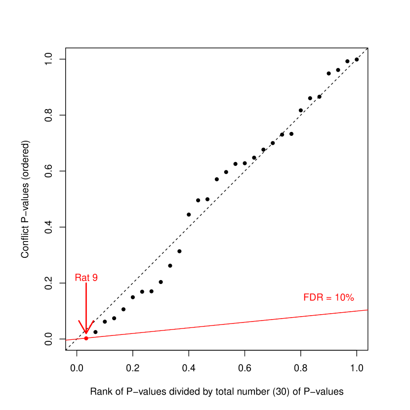
Figure 2: $P$-values from rat growth data. The Benjamini and Hochberg criterion is superimposed as a red line, identifying rat 9 as being divergent.

Figure 1 shows a scatterplot of MCMC versus INLA $p$-values. There is not any substantial difference between the MCMC and INLA results. Figure 2 shows the empirical distribution of the resulting $p$-values. Rat number 9 is identified as an “outlier” ($p$=0.0021) at a false discovery rate (Benjamini and Hochberg,, 1995) of 10%.

The total INLA run time for this example was 8.3 seconds, with the initial INLA run taking 2.5 seconds and the node-splitting using inla.cut (see Section 3) taking 5.8 seconds. A machine with 12 Intel Xeon X5680 3.33 GHz CPUs and 99 GB RAM was used. The MCMC run time using the same hardware, running JAGS and two chains of 200,000 iterations each (discarding the first 100,000 iterations), was 34 minutes, so INLA was nearly 250 times faster than MCMC for this example. While it is of course difficult to know for how long it is necessary to run an MCMC algorithm, investigation of convergence diagnostics from the MCMC run indicates that the stated iterations/burn-in is not excessive.

4.2 Low birth weight in Georgia

In this example, we study the “Georgia low birth weight” disease mapping data set from Section 11.2.1 of Lawson, (2013). Different analyses of these data using INLA are described in Blangiardo et al., (2013). The data consist of counts of children born with low birth weight (defined as less than 2500 g) for the 159 counties of the state of Georgia, USA, for the 11 years 2000-2010. Let $y_{ij}$ be the count for county $i=1,\ldots,159$, year $j=1,\ldots,11$, and let $t_{j}=j-5$ be the centered year index. A possible model is then

$$y_{ij} \sim \text{Poisson}(E_{ij}\exp(\eta_{ij})),$$

$$\eta_{ij} = \mu+u_{i}+v_{i}+\beta t_{j},$$ (9)

where $E_{ij}$ is the total number of births, and $u_{i}$ and $v_{i}$ are together given a Besag-York-Mollie (BYM) model (Besag et al.,, 1991). In the BYM model, the spatially structured random effect $u_{i}$ is given a intrinsic conditionally independent autoregressive structure (iCAR), with $u_{i}|u_{j\neq i}\sim N(n_{i}^{-1}\sum_{\mathcal{N}_{i}}u_{j},n_{i}^{-1}\sigma_{v}^{2})$, where $n_{i}$ is the number of neighbors (sharing a common border) with county $i$, and $\mathcal{N}_{i}$ denotes the set of neighbors of $i$. The $v_{i}$ are residual unstructured effects, independent and identically distributed $N(0,\sigma_{u})$. The INLA default low-informative priors are defined on the hyperparameters $\theta_{u}=\log\sigma_{u}^{-2}$ and $\theta_{v}=\log\sigma_{v}^{-2}$: both $\theta_{u}$ and $\theta_{v}$ are given Gamma$(1,0.0005)$ priors.

For this model, traditional model-check diagnostics are either on the (county, year) level (checking the fit for each individual count $y_{ij}$) or on the overall model (as we could do with standard goodness-of-fit tests). However, using the node-splitting methodology we can also either

1. check the model adequacy by county, or

2. check the model adequacy by year,

simply by grouping by county or year, respectively.

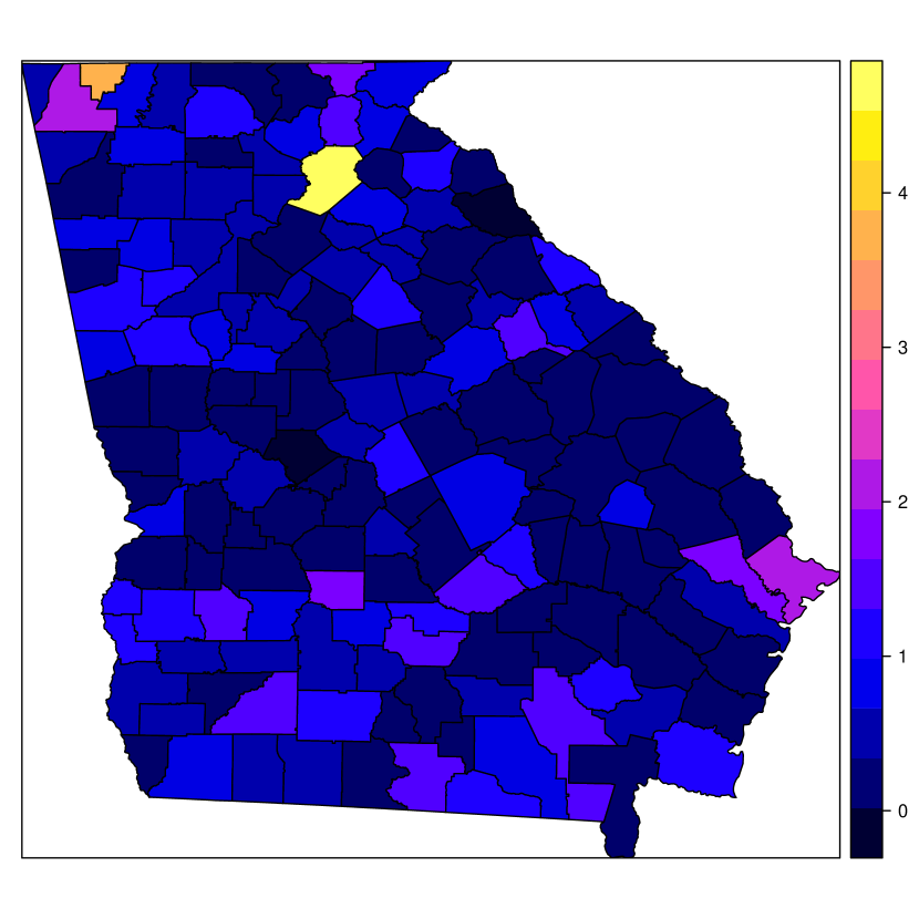
Figure 3: Map of $-\log_{10}$ of $p$-values from spatial split of low birth weight model.

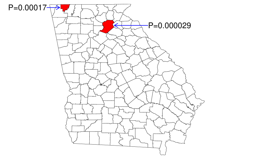
Figure 4: The two “outlier” counties identified as not conforming to the model.

Figures 3 and 4 show the results from the (spatial) split by county. Two counties are identified as divergent at a 10% false discovery rate (FDR) level: Hall and Catoosa county, with $p$-values of 0.000029 and 0.00017, respectively.

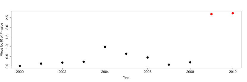
Figure 5: Time series of $-\log_{10}$ of $p$-values from temporal (yearly) split of low birth weight model. The two last years (marked in red) are identified as outliers.

It is also interesting to study the model adequacy by year: Are any of the years (from 2000-2010) identified as outliers? Figure 5 shows the results ($-\log_{10}$ of $p$-values) from node-split when we group by year. We see that the last two years, 2009 and 2010, are identified as divergent, with $p$-values of 0.0022 and 0.0020, respectively. This suggests that the assumption of a linear time trend in model (9) needs some amendment.

The run time (using the same hardware as in Section 4.1) was approximately four seconds for the initial INLA run, 30 seconds for the split by year, and approximately five minutes for the split by county. We did not implement any MCMC algorithm for this example.

5 Discussion

Although our aim has been to provide a general, easy-to-use implementation, there are some limitations. First, we currently assume that the grouping is “linear” in the sense of always comparing group $i$, say, with all remaining groups (“$-i$”). To implement the method for the case of network meta-analysis, it would be necessary to extend the implementation to the more general case where group $i$ might be compared with some, but not all, of the remaining groups, and the list of “remaining groups” might change arbitrarily with $i$. Second, we only consider conflict detection based on the linear predictor of the model; in some cases it might be necessary to consider other parameters. However, this would make it more challenging to provide a general implementation. Third, we restrict to the class of latent Gaussian models, but this is of course more a limitation of the INLA methodology itself and not of the model criticism method as such. Finally, as described above, the method (as currently implemented) relies on an assumption of approximate multivariate normality of the posterior linear predictor. As discussed in Section 3.2.3 on page 384 of Presanis et al., (2013), there are ways to avoid this assumption, at the cost of a higher computational load. For example, if we only want to assume a symmetric and unimodal (but not necessarily normal) posterior density, an alternative test can be devised based on sampling from the posterior and using Mahalanobis distances. Since R-INLA provides functionality for quickly producing independent samples from the approximated joint posterior, the Mahalanobis distance based approach could potentially be implemented within our approach. However, in our experience the posterior distribution of the linear predictor is nearly always sufficiently close to normal; thus, our judgment has been that using the Mahalanobis-based p-values was not worth the extra computational effort, and it is not currently implemented. Nevertheless, if there is a popular demand, this functionality might be added in a future version of the software.

The method is cross-validatory in nature and avoids “using the data twice”, a well-known problem with posterior predictive $p$-values and related methods Bayarri and Castellanos, (2007). Nevertheless, it would be a useful topic for further study to consider both the power of our conflict detection tests, as well as the “calibration” in the sense that $p$-values from a true model should be uniformly distributed (see Gåsemyr, (2016) for some recent work on the calibration of node level conflict measures). In particular, in some cases the method may not detect a "practically significant" conflict due to insufficient power. Power (e.g. with FDR thresholding) has not yet been investigated systematically so far, and this could potentially be carried out in a simulation study with INLA, whereas MCMC would be too slow to do this. Simulation studies could also be useful for assessing the calibration issue mentioned above, i.e. whether $p$-values are really always uniform under no conflict.

To account for the multiple testing issues generated by considering many groups and performing a test for each group, we have simply used FDR. FDR correction provides a convenient and well-understood methodology for dealing with multiple testing. However, it could still potentially be useful to employ multiple testing methodology that is more specifically geared to the group-wise model checking tests used here. See Presanis et al., (2017) for some work in this direction.

Finally, it could be useful to provide graphical or more general numerical measures of fit in addition to the conflict $p$-values, in order to obtain further insight into the reasons for any discovered lack of fit, for example, using the approach of Scheel et al., (2011). We leave this as an interesting topic for further work.

References

- Azzalini and Capitanio, (1999) Azzalini, A. and Capitanio, A. (1999). Statistical applications of the multivariate skew normal distribution. Journal of the Royal Statistical Society: Series B (Statistical Methodology), 61(3):579–602.
- Bayarri and Castellanos, (2007) Bayarri, M. and Castellanos, M. (2007). Bayesian checking of the second levels of hierarchical models. Statistical Science, 22(3):322–343.
- Benjamini and Hochberg, (1995) Benjamini, Y. and Hochberg, Y. (1995). Controlling the false discovery rate: a practical and powerful approach to multiple testing. Journal of the Royal Statistical Society Series B (Methodological), pages 289–300.
- Besag et al., (1991) Besag, J., York, J., and Mollié, A. (1991). Bayesian image restoration, with two applications in spatial statistics. Annals of the Institute of Statistical Mathematics, 43(1):1–20.
- Blangiardo et al., (2013) Blangiardo, M., Cameletti, M., Baio, G., and Rue, H. (2013). Spatial and spatio-temporal models with R-INLA. Spatial and Spatio-temporal Epidemiology, 7:39–55.
- Carpenter et al., (2017) Carpenter, B., Gelman, A., Hoffman, M., Lee, D., Goodrich, B., Betancourt, M., Brubaker, M. A., Guo, J., Li, P., and Riddell, A. (2017). STAN: a probabilistic programming language. Journal of Statistical Software, 76(1).
- Dawid, (1984) Dawid, A. P. (1984). Statistical theory: the prequential approach. Journal of the Royal Statistical Society. Series A (General), 147:278–292.
- Dias et al., (2010) Dias, S., Welton, N., Caldwell, D., and Ades, A. (2010). Checking consistency in mixed treatment comparison meta-analysis. Statistics in Medicine, 29(7-8):932–944.
- Ferkingstad and Rue, (2015) Ferkingstad, E. and Rue, H. (2015). Improving the INLA approach for approximate Bayesian inference for latent Gaussian models. Electronic Journal of Statistics, 9(2):2706–2731.
- Gåsemyr, (2016) Gåsemyr, J. (2016). Uniformity of node level conflict measures in Bayesian hierarchical models based on directed acyclic graphs. Scandinavian Journal of Statistics, 43(1):20–34.
- Gåsemyr and Natvig, (2009) Gåsemyr, J. and Natvig, B. (2009). Extensions of a conflict measure of inconsistencies in Bayesian hierarchical models. Scandinavian Journal of Statistics, 36(4):822–838.
- Gelfand et al., (1990) Gelfand, A. E., Hills, S. E., Racine-Poon, A., and Smith, A. F. (1990). Illustration of Bayesian inference in normal data models using Gibbs sampling. Journal of the American Statistical Association, 85(412):972–985.
- Gelman et al., (1996) Gelman, A., Meng, X.-L., and Stern, H. (1996). Posterior predictive assessment of model fitness via realized discrepancies. Statistica Sinica, 6:733–760.
- Held et al., (2010) Held, L., Schrödle, B., and Rue, H. (2010). Posterior and cross-validatory predictive checks: a comparison of MCMC and INLA. In Statistical Modelling and Regression Structures, pages 91–110. Springer.
- Lawson, (2013) Lawson, A. B. (2013). Bayesian Disease Mapping: Hierarchical Modeling in Spatial Epidemiology. CRC press.
- Lumley, (2002) Lumley, T. (2002). Network meta-analysis for indirect treatment comparisons. Statistics in Medicine, 21(16):2313–2324.
- Lunn et al., (2009) Lunn, D., Spiegelhalter, D., Thomas, A., and Best, N. (2009). The BUGS project: evolution, critique and future directions. Statistics in Medicine, 28(25):3049–3067.
- Marshall and Spiegelhalter, (2007) Marshall, E. C. and Spiegelhalter, D. J. (2007). Identifying outliers in Bayesian hierarchical models: a simulation-based approach. Bayesian Analysis, 2(2):409–444.
- Martins et al., (2013) Martins, T. G., Simpson, D., Lindgren, F., and Rue, H. (2013). Bayesian computing with INLA: new features. Computational Statistics & Data Analysis, 67:68 – 83.
- McCullagh and Nelder, (1989) McCullagh, P. and Nelder, J. A. (1989). Generalized Linear Models. Chapman & Hall, 2nd edition.
- Pettit, (1990) Pettit, L. I. (1990). The conditional predictive ordinate for the normal distribution. Journal of the Royal Statistical Society: Series B (Methodological), 52:175–184.
- Plummer, (2015) Plummer, M. (2015). Cuts in Bayesian graphical models. Statistics and Computing, 25(1):37–43.
- Plummer, (2016) Plummer, M. (2016). JAGS version 4.2.0. http://mcmc-jags.sourceforge.net.
- Presanis et al., (2017) Presanis, A. M., Ohlssen, D., Cui, K., Rosinska, M., and De Angelis, D. (2017). Conflict diagnostics for evidence synthesis in a multiple testing framework. arXiv preprint arXiv:1702.07304.
- Presanis et al., (2013) Presanis, A. M., Ohlssen, D., Spiegelhalter, D. J., De Angelis, D., et al. (2013). Conflict diagnostics in directed acyclic graphs, with applications in Bayesian evidence synthesis. Statistical Science, 28(3):376–397.
- Rue and Held, (2005) Rue, H. and Held, L. (2005). Gaussian Markov Random Fields: Theory and Applications. CRC Press.
- Rue et al., (2009) Rue, H., Martino, S., and Chopin, N. (2009). Approximate Bayesian inference for latent Gaussian models by using integrated nested Laplace approximations (with discussion). Journal of the Royal Statistical Society: Series B (Statistical methodology), 71(2):319–392.
- Rue et al., (2017) Rue, H., Riebler, A., Sørbye, S. H., Illian, J. B., Simpson, D. P., and Lindgren, F. K. (2017). Bayesian computing with INLA: A review. Annual Review of Statistics and Its Application, 4:395–421.
- Sauter and Held, (2015) Sauter, R. and Held, L. (2015). Network meta-analysis with integrated nested Laplace approximations. Biometrical Journal, 57:1038–1050.
- Scheel et al., (2011) Scheel, I., Green, P. J., and Rougier, J. C. (2011). A graphical diagnostic for identifying influential model choices in Bayesian hierarchical models. Scandinavian Journal of Statistics, 38(3):529–550.
- Simpson et al., (2017) Simpson, D. P., Rue, H., Martins, T. G., Riebler, A., and Sørbye, S. H. (2017). Penalising model component complexity: a principled, practical approach to constructing priors. Statistical Science, 32(1):1–28.
- Spiegelhalter et al., (2002) Spiegelhalter, D. J., Best, N. G., Carlin, B. P., and Van Der Linde, A. (2002). Bayesian measures of model complexity and fit. Journal of the Royal Statistical Society: Series B (Statistical Methodology), 64(4):583–639.
- Tierney and Kadane, (1986) Tierney, L. and Kadane, J. B. (1986). Accurate approximations for posterior moments and marginal densities. Journal of the American Statistical Association, 81(393):82–86.
- Vehtari et al., (2016) Vehtari, A., Gelman, A., and Gabry, J. (2016). Practical Bayesian model evaluation using leave-one-out cross-validation and WAIC. Statistics and Computing, pages 1–20.
- Watanabe, (2010) Watanabe, S. (2010). Asymptotic equivalence of Bayes cross validation and widely applicable information criterion in singular learning theory. Journal of Machine Learning Research, 11(Dec):3571–3594.