Interaction of martensitic microstructures in adjacent grains

Abstract.

It is often observed that martensitic microstructures in adjacent polycrystal grains are related. For example, micrographs of Arlt [1] (one reproduced in [10, p225]) exhibit propagation of layered structures across grain boundaries in the cubic-to-tetragonal phase transformation in $\rm BaTiO_{3}$. Such observations are related to requirements of compatibility of the deformation at the grain boundary. Using a generalization of the Hadamard jump condition, this is explored in the nonlinear elasticity model of martensitic transformations for the case of a bicrystal with suitably oriented columnar geometry, in which the microstructure in both grains is assumed to involve just two martensitic variants, with a planar or non-planar interface between the grains.

empty

Keywords: Bicrystal, compatibility, grain boundary, Hadamard jump condition.

1. Description of problem

Consider a bicrystal consisting of two columnar grains $\Omega_{1}=\omega_{1}\times(0,d)$ (grain 1), $\Omega_{2}=\omega_{2}\times(0,d)$ (grain 2), where $d>0$ and $\omega_{1},\omega_{2}\subset\mathbb{R}^{2}$ are bounded Lipschitz domains whose boundaries $\partial\omega_{1},\partial\omega_{2}$ intersect nontrivially, so that $\partial\omega_{1}\cap\partial\omega_{2}$ contains points in the interior $\omega$ of $\overline{\omega}_{1}\cup\overline{\omega}_{2}$ (see Fig. 1). Let $\Omega=\omega\times(0,d)$. The interface between the grains is the set $\partial\Omega_{1}\cap\partial\Omega_{2}\cap\Omega=(\partial\omega_{1}\cap\partial\omega_{2}\cap\omega)\times(0,d)$. Since by assumption the boundaries $\partial\omega_{1},\partial\omega_{2}$ are locally the graphs of Lipschitz functions, and such functions are differentiable almost everywhere, the interface has at almost every point (with respect to area) a well-defined normal ${\bf n}(\theta)=(\cos\theta,\sin\theta,0)$ in the $(x_{1},x_{2})$ plane. We say that the interface is planar if it is contained in some plane $\{{\bf x}\cdot{\bf n}=k\}$ for a fixed normal ${\bf n}$ and constant $k$.

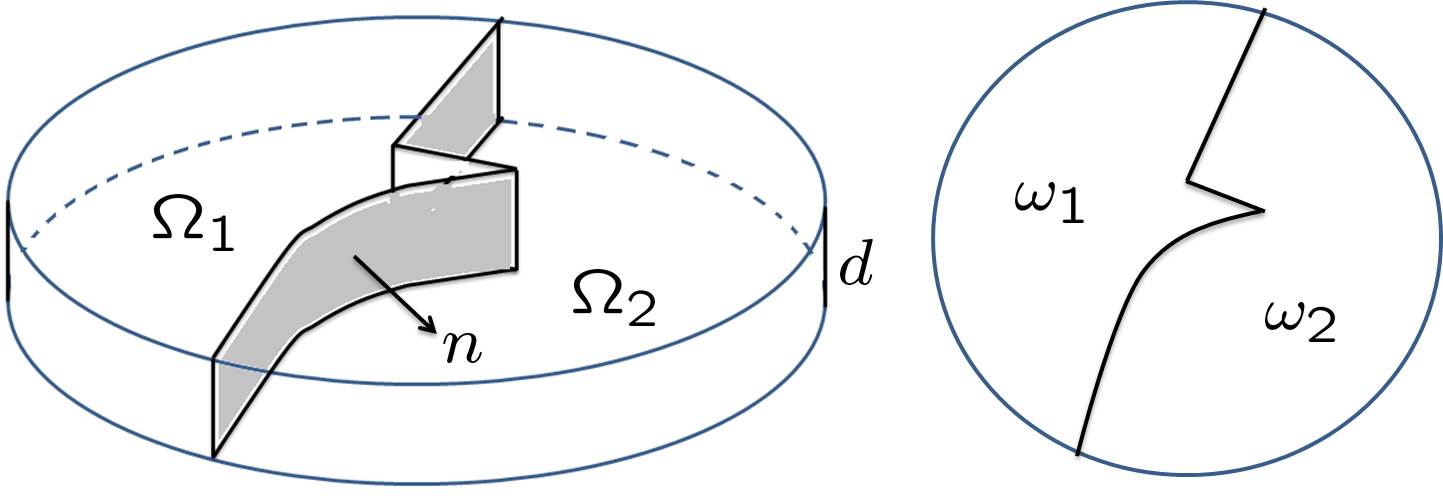
Figure 1. Bicrystal consisting of two grains $\Omega_{1}=\omega_{1}\times(0,d),\Omega_{2}=\omega_{2}\times(0,d).$

We use the nonlinear elasticity model of martensitic transformations from [6, 8], with corresponding free-energy density $\psi(\nabla{\bf y},\theta)$ for a single crystal at temperature $\theta$ and deformation ${\bf y}={\bf y}({\bf x})$ with respect to undistorted austenite at the critical temperature $\theta_{c}$ at which the austenite and martensite have the same free energy. We denote by $\mathbb{R}^{n\times n}_{+}$ the set of real $n\times n$ matrices ${\bf A}$ with $\det{\bf A}>0$, and by $SO(n)$ the set of rotations in $\mathbb{R}^{n}$. At a fixed temperature $\theta<\theta_{c}$, we suppose that

$$K=SO(3){\bf U}_{1}\cup SO(3){\bf U}_{2}$$ (1.1)

is the set of ${\bf A}\in\mathbb{R}^{3\times 3}_{+}$ minimizing $\psi({\bf A},\theta)$, where ${\bf U}_{1}={\rm diag}\,(\eta_{2},\eta_{1},\eta_{3})$, ${\bf U}_{2}={\rm diag}\,(\eta_{1},\eta_{2},\eta_{3})$ and $\eta_{2}>\eta_{1}>0$, $\eta_{3}>0$. This corresponds to a tetragonal to orthorhombic phase transformation (see [10, Table 4.6]), or to an orthorhombic to monoclinic transformation in which the transformation strain involves stretches of magnitudes $\eta_{1},\eta_{2}$ with respect to perpendicular directions lying in the plane of two of the orthorhombic axes and making an angle of $\pi/4$ with respect to these axes. Alternatively, for example, taking $\eta_{3}=\eta_{1}$ the analysis of this paper can be viewed as applying to a cubic to tetragonal transformation under the a priori assumption that only two variants are involved in the microstructure.

We suppose that $\Omega_{1}$ has cubic axes in the coordinate directions ${\bf e}_{1},{\bf e}_{2},{\bf e}_{3}$, while in $\Omega_{2}$ the cubic axes are rotated through an angle $\alpha$ about ${\bf e}_{3}$. By adding a constant to $\psi$ we may assume that $\psi({\bf A},\theta)=0$ for ${\bf A}\in K$. Then a zero-energy microstructure corresponds to a gradient Young measure $(\nu_{\bf x})_{{\bf x}\in\Omega}$ such that

$${\rm supp}\,\nu_{\bf x}\subset K\mbox{ for a.e. }{\bf x}\in\Omega_{1},\;\;{\rm supp}\,\nu_{\bf x}\subset K{\bf R}_{\alpha}\mbox{ for a.e. }{\bf x}\in\Omega_{2},$$ (1.2)

where

$${\bf R}_{\alpha}=\left(\begin{array}[]{lll}\cos\alpha&-\sin\alpha&0\\ \sin\alpha&\cos\alpha&0\\ 0&0&1\end{array}\right).$$

It is easily shown that $K{\bf R}_{\alpha}=K$ if and only if $\alpha=n\pi/2$ for some integer $n$, and that $K{\bf R}_{\alpha+\pi/2}=K{\bf R}_{\alpha}$. We thus assume that $0<\alpha<\frac{\pi}{2}$, since this covers all nontrivial cases.

As remarked in [5], by a result from [9] there always exists a zero-energy microstructure constructed using laminates, with gradient Young measure $\nu_{\bf x}=\nu$ satisfying (1.2) that is independent of $x$ and has macroscopic deformation gradient $\bar{\nu}=\int_{\mathbb{R}^{3\times 3}_{+}}{\bf A}\,d\nu({\bf A})=(\det{\bf U}_{1}){\bf 1}$. Our aim is to give conditions on the deformation parameters $\eta_{1},\eta_{2},\eta_{3}$, the rotation angle $\alpha$ and the grain geometry which ensure that any zero-energy microstructure has a degree of complexity in each grain, in the sense that it does not correspond to a pure variant with constant deformation gradient in either of the grains.

2. Rank-one connections between energy wells

Let ${\bf U}={\bf U}^{T}>0$, ${\bf V}={\bf V}^{T}>0$. We say that the energy wells ${\rm SO}(3){\bf U}$, ${\rm SO}(3){\bf V}$ are rank-one connected if there exist ${\bf R},{\bf Q}\in SO(3)$, ${\bf a},{\bf n}\in\mathbb{R}^{3}$, $|{\bf n}|=1$ with ${\bf R}{\bf U}={\bf Q}{\bf V}+{\bf a}\otimes{\bf n}$, where without loss of generality we can take ${\bf Q}={\bf 1}$. By the Hadamard jump condition this is equivalent to the existence of a continuous piecewise affine map ${\bf y}$ whose gradient $\nabla{\bf y}$ takes constant values ${\bf A}\in SO(3){\bf U}$ and ${\bf B}\in SO(3){\bf V}$ on either side of a plane with normal ${\bf n}$. The following is an apparently new version of a well-known result (see, for example, [6, Prop. 4], [2, Theorem 2.1], [12]), giving necessary and sufficient conditions for two wells to be rank-one connected. A similar statement was obtained by Mardare [13].

Lemma 1.

Let ${\bf U}={\bf U}^{T}>0$, ${\bf V}={\bf V}^{T}>0$. Then ${\rm SO}(3){\bf U}$, ${\rm SO}(3){\bf V}$ are rank-one connected if and only if

$${\bf U}^{2}-{\bf V}^{2}=\gamma({\bf m}\otimes{\bf n}+{\bf n}\otimes{\bf m})$$ (2.1)

for unit vectors ${\bf m}$, ${\bf n}$ and some $\gamma\neq 0$. For suitable ${\bf a}_{1},{\bf a}_{2}\in\mathbb{R}^{3}$ and ${\bf R}_{1},{\bf R}_{2}\in{\rm SO}(3)$, the rank-one connections between ${\bf V}$ and ${\rm SO}(3){\bf U}$ are given by

$${\bf R}_{1}{\bf U}={\bf V}+{\bf a}_{1}\otimes{\bf n},\quad{\bf R}_{2}{\bf U}={\bf V}+{\bf a}_{2}\otimes{\bf m}.$$ (2.2)

We omit the proof, which is not difficult. The main point of the lemma is that the normals corresponding to the rank-one connections are the vectors appearing in (2.1). An interesting consequence is that if ${\bf U},{\bf V}$ correspond to martensitic variants, so that ${\bf V}={\bf Q}^{T}{\bf U}{\bf Q}$ for some ${\bf Q}\in SO(3)$, then, taking the trace in (2.1) shows that the two possible normals are orthogonal (see [2, Theorem 2.1]).

Using Lemma 1 we can calculate the rank-one connections between $K$ and $K{\bf R}_{\alpha}$. For example, for the rank-one connections between ${\rm SO}(3)\,{\bf U}_{1}$ and ${\rm SO}(3)\,{\bf U}_{1}{\bf R}_{\alpha}$ we find that

$${\bf U}_{1}^{2}-{\bf R}_{\alpha}^{T}{\bf U}_{1}^{2}{\bf R}_{\alpha}\,=(\eta_{2}^{2}-\eta_{1}^{2})\sin\alpha\,({\bf m}\otimes{\bf n}+{\bf n}\otimes{\bf m})$$ (2.3)

where ${\bf n}=(\sin(\alpha/2),\cos(\alpha/2),0)$, ${\bf m}=(\cos(\alpha/2),-\sin(\alpha/2),0)$ so that the two possible normals ${\bf n}=(n_{1},n_{2},0)$ satisfy $\tan\alpha=2n_{1}n_{2}/(n_{2}^{2}-n_{1}^{2})$. Swapping $\eta_{1}$ and $\eta_{2}$ we see that the possible normals for rank-one connections between ${\rm SO}(3)\,{\bf U}_{2}$ and ${\rm SO}(3)\,{\bf U}_{2}{\bf R}_{\alpha}$ are the same. Similarly, we find that the possible normals for rank-one connections between ${\rm SO}(3){\bf U}_{1}$ and ${\rm SO}(3){\bf U}_{2}{\bf R}_{\alpha}$ or between ${\rm SO}(3){\bf U}_{2}$ and ${\rm SO}(3){\bf U}_{1}{\bf R}_{\alpha}$ satisfy $\tan\alpha=(n_{1}^{2}-n_{2}^{2})/2n_{1}n_{2}$.

3. Main results

Suppose there exists a gradient Young measure of the form (1.2) such that $\nu_{\bf x}=\delta_{\bf F}$ for a.e. ${\bf x}\in\Omega_{1}$ for some ${\bf F}\in K$, corresponding to a pure variant in grain 1. It follows that the corresponding macroscopic gradient $\nabla{\bf y}({\bf x})=\bar{\nu}_{\bf x}=\int_{M^{3\times 3}_{+}}{\bf A}d\nu_{x}({\bf A})$ satisfies

$$\nabla{\bf y}({\bf x})={\bf F}\mbox{ for a.e. }{\bf x}\in\Omega_{1},\;\;\nabla{\bf y}({\bf x})\in(K{\bf R}_{\alpha})^{\rm qc}\mbox{ for a.e. }{\bf x}\in\Omega_{2},$$ (3.1)

where $E^{\rm qc}$ denotes the quasiconvexification of a compact set $E\subset\mathbb{R}^{3\times 3}$, that is the set of possible macroscopic deformation gradients corresponding to microstructures using gradients in $E$. As determined in [6, Theorem 5.1] (and more conveniently in [10, p155]) $K^{\rm qc}$ consists of those ${\bf A}\in\mathbb{R}_{+}^{3\times 3}$ with

$${\bf A}^{T}{\bf A}=\left(\begin{array}[]{ccc}a&c&0\\ c&b&0\\ 0&0&\eta_{3}^{2}\end{array}\right)\mbox{ and }\;(a,b,c)\in P,$$ (3.5)

$$P=\{(a,b,c):a>0,\;b>0,\;ab-c^{2}=\eta_{1}^{2}\eta_{2}^{2},\;a+b+|2c|\leq\eta_{1}^{2}+\eta^{2}_{2}\},$$ (3.6)

and is equal to the polyconvexification $K^{pc}$ of $K$. It follows that $(K{\bf R}_{\alpha})^{\rm qc}=K^{\rm qc}{\bf R}_{\alpha}=K^{\rm pc}{\bf R}_{\alpha}$. The proof of (3.5) shows also that the quasiconvexification $\tilde{K}^{\rm qc}$ of $\tilde{K}=SO(2)\tilde{\bf U}_{1}\cup SO(2)\tilde{\bf U}_{2}$, where $\tilde{\bf U}_{1}=\left(\begin{array}[]{cc}\eta_{2}&0\\ 0&\eta_{1}\end{array}\right)$, $\tilde{\bf U}_{2}=\left(\begin{array}[]{cc}\eta_{1}&0\\ 0&\eta_{2}\end{array}\right)$, is equal to $\tilde{K}^{\rm pc}$ and is given by the set of $\tilde{\bf A}\in\mathbb{R}^{2\times 2}_{+}$ such that $\tilde{\bf A}^{T}\tilde{\bf A}=\left(\begin{array}[]{cc}a&c\\ c&b\end{array}\right)\mbox{ for }(a,b,c)\in P.$

Let ${\bf x}_{0}=(\tilde{\bf x}_{0},\delta)$, where $\tilde{\bf x}_{0}\in\partial\omega_{1}\cap\partial\omega_{2}\cap\omega$, $0<\delta<d$, be such that the interface has a well-defined normal ${\bf n}=(\cos\theta,\sin\theta,0)=(\tilde{\bf n},0)$ at ${\bf x}_{0}$. By [7], there exists $\varepsilon>0$ such that in ${\mathcal{U}}:=B(\tilde{\bf x}_{0},\varepsilon)\times(\delta-\varepsilon,\delta+\varepsilon)$, $0<\varepsilon<\delta$, the map ${\bf y}$ is a plane strain, that is

$${\bf y}({\bf x})={\bf R}(z_{1}(x_{1},x_{2}),z_{2}(x_{1},x_{2}),\eta_{3}x_{3}+\gamma)\mbox{ for a.e. }{\bf x}\in\mathcal{U}$$ (3.7)

for some ${\bf R}\in SO(3)$, ${\bf z}:B(\tilde{\bf x}_{0},\varepsilon)\to\mathbb{R}^{2}$ and $\gamma\in\mathbb{R}$, where $B(\tilde{\bf x}_{0},\varepsilon)$ denotes the open ball in $\mathbb{R}^{2}$ with centre $\tilde{\bf x}_{0}$ and radius $\varepsilon$. Without loss of generality we can take ${\bf R}={\bf 1}$. Then, for $\tilde{\bf x}=(x_{1},x_{2})\in B(\tilde{\bf x}_{0},\varepsilon)$ we have

$$\nabla{\bf z}(\tilde{\bf x})=\tilde{\bf F}\in\tilde{K}\mbox{ for a.e. }\tilde{\bf x}\in\omega_{1},\;\;\nabla{\bf z}(\tilde{\bf x})\in(\tilde{K}\tilde{\bf R}_{\alpha})^{\rm pc}=\tilde{K}^{\rm pc}\tilde{\bf R}_{\alpha}\mbox{ for a.e. }\tilde{\bf x}\in\omega_{2},$$ (3.8)

where $\tilde{\bf R}_{\alpha}=\left(\begin{array}[]{cc}\cos\alpha&-\sin\alpha\\ \sin\alpha&\cos\alpha\end{array}\right)$. By a two-dimensional generalization of the Hadamard jump condition proved in [3] this implies that there exists $\tilde{\bf A}\in(\tilde{K}\tilde{\bf R}_{\alpha})^{\rm pc}$ such that

$$\tilde{\bf F}-\tilde{\bf A}=\tilde{\bf a}\otimes\tilde{\bf n}$$ (3.9)

for some $\tilde{\bf a}\in\mathbb{R}^{2}$. Conversely, if the interface is planar with normal ${\bf n}=(\tilde{\bf n},0)$, then the existence of $\tilde{\bf A}\in(\tilde{K}\tilde{\bf R}_{\alpha})^{\rm pc}$ satisfying (3.9) implies the existence of a gradient Young measure $\nu=(\nu_{\bf x})_{{\bf x}\in\Omega}$ satisfying (3.1). Indeed there then exists a sequence of gradients $\nabla{\bf z}^{(j)}$ generating a gradient Young measure $(\mu_{\tilde{\bf x}})_{\tilde{\bf x}\in\omega}$ such that

$$\bar{\mu}_{\tilde{\bf x}}=\tilde{\bf F}\mbox{ for a.e. }\tilde{\bf x}\in\omega_{1},\;\;\bar{\mu}_{\tilde{\bf x}}=\tilde{\bf A}\mbox{ for a.e. }\tilde{\bf x}\in\omega_{2},$$ (3.10)

and then $\nabla{\bf y}^{(j)}({\bf x})=\left(\begin{array}[]{ccc}z^{(j)}_{1,1}&z^{(j)}_{1,2}&0\\ z^{(j)}_{2,1}&z^{(j)}_{2,2}&0\\ 0&0&\eta_{3}\end{array}\right)$ generates such a gradient Young measure.

It turns out that we can say exactly when it is possible to solve (3.9). Set $\tau:=\eta_{2}/\eta_{1}>1$, $s^{*}=(\tau^{4}-1)/(\tau^{4}+1)$ and define for $0\leq s\leq 1$ the $C^{1}$ convex increasing function

$$f(s):=\left\{\begin{array}[]{cc}(\tau^{4}+1-2\tau^{2}\sqrt{1-s^{2}})/(\tau^{4}-1)&\mbox{if }s\leq s^{*},\\ s&\mbox{if }s>s^{*}.\end{array}\right.$$ (3.13)

Theorem 2.

There exist $\tilde{\bf F}\in\tilde{K}$ and $\tilde{\bf A}\in\tilde{K}^{\rm pc}{\bf R}_{\alpha}$ with $\tilde{\bf F}-\tilde{\bf A}=\tilde{\bf a}\otimes\tilde{\bf n}$ for $\tilde{\bf n}=(\cos\theta,\sin\theta)$ and some $\tilde{\bf a}\in\mathbb{R}^{2}$ if and only if

$$|\cos 2\theta|\leq f(|\cos 2(\alpha+\theta)|).$$ (3.14)

Proof.

It is easily checked that the existence of $\tilde{\bf F}\in SO(3)\tilde{\bf U}_{i}$ and $\tilde{\bf A}$ is equivalent to the existence of $(a,b,c)\in P$ such that $|\tilde{\bf U}_{i}\tilde{\bf n}^{\perp}|^{2}=aN_{1}^{2}+bN_{2}^{2}+2cN_{1}N_{2}$, where $\tilde{\bf n}^{\perp}=(-n_{2},n_{1})$ and ${\bf N}=(N_{1},N_{2})=\tilde{\bf R}_{\alpha}\tilde{\bf n}^{\perp}$. That is

$$\mbox{ either }n_{1}^{2}\eta_{1}^{2}+n_{2}^{2}\eta_{2}^{2}\mbox{ or }n_{2}^{2}\eta_{1}^{2}+n_{1}^{2}\eta_{2}^{2}\;\;\in[m_{-}({\bf N}),m_{+}({\bf N})],$$ (3.15)

where $m_{\pm}({\bf N})=\mathop{\small\min}\limits^{\textstyle\small\max}_{(a,b,c)\in P}(aN_{1}^{2}+bN_{2}^{2}+2cN_{1}N_{2})$. Changing variables to $x=a+b$ and $y=a-b$ we find that $m_{+}({\bf N})=\max_{(x,y)\in P_{2}}\psi_{+}(x,y)$, $m_{-}({\bf N})=\min_{(x,y)\in P_{2}}\psi_{-}(x,y)$, where

$$2\psi_{\pm}(x,y)=x+y(N_{1}^{2}-N_{2}^{2})\pm 2|N_{1}N_{2}|\sqrt{x^{2}-y^{2}-4\eta_{1}^{2}\eta_{2}^{2}},$$ (3.16)

$$P_{2}=\Big{\{}(x,y)\in\mathbb{R}^{2}:|y|\leq\eta_{2}^{2}-\eta_{1}^{2}\mbox{ and }\sqrt{y^{2}+4\eta_{1}^{2}\eta_{2}^{2}}\leq x\leq\frac{y^{2}+4\eta_{1}^{2}\eta_{2}^{2}+(\eta_{1}^{2}+\eta_{2}^{2})^{2}}{2(\eta_{1}^{2}+\eta_{2}^{2})}\Big{\}}.$$

The region $P_{2}$ is bounded by the two arcs $C_{1}:=\{x=\sqrt{y^{2}+4\eta_{1}^{2}\eta_{2}^{2}}\}$ and $C_{2}:=\{x=(y^{2}+4\eta_{1}^{2}\eta_{2}^{2}+(\eta_{1}^{2}+\eta_{2}^{2})^{2})/(2(\eta_{1}^{2}+\eta_{2}^{2}))\}$, defined for $|y|\leq\eta^{2}_{2}-\eta_{1}^{2}$, which intersect at the points $(x,y)=(\eta_{1}^{2}+\eta_{2}^{2},\pm(\eta_{2}^{2}-\eta_{1}^{2}))$. Note that $\psi_{\pm}(x,y)$ have no critical points in the interior of $P_{2}$. In fact it is immediate that $\nabla\psi_{+}$ cannot vanish, while $\nabla\psi_{-}(x,y)=0$ leads to $y=x(N_{2}^{2}-N_{1}^{2})$ and hence to the contradiction $0=x^{2}-y^{2}-4x^{2}N_{1}^{2}N_{2}^{2}=4\eta_{1}^{2}\eta_{2}^{2}>0$. Thus the maximum and minimum of $\psi_{\pm}(x,y)$ are attained on either $C_{1}$ or $C_{2}$. After some calculations we obtain

$$m_{+}({\bf N}) = \frac{1}{2}(\eta_{1}^{2}+\eta_{2}^{2}+(\eta_{2}^{2}-\eta_{1}^{2})|N_{1}^{2}-N_{2}^{2}|),$$

$$m_{-}({\bf N}) = \left\{\begin{array}[]{ll}\frac{\eta_{1}^{2}\eta_{2}^{2}}{\eta_{1}^{2}+\eta_{2}^{2}}\Big{(}1+\sqrt{1-|N_{1}^{2}-N_{2}^{2}|^{2}}\Big{)}&\mbox{ if }\>|N_{1}^{2}-N_{2}^{2}|\leq s^{*},\\ \frac{1}{2}(\eta_{1}^{2}+\eta_{2}^{2}-|N_{1}^{2}-N_{2}^{2}|(\eta_{2}^{2}-\eta_{1}^{2}))&\mbox{ if }\>|N_{1}^{2}-N_{2}^{2}|\geq s^{*}.\end{array}\right.$$

Noting that $m_{-}({\bf N})\leq\frac{1}{2}(\eta_{1}^{2}+\eta_{2}^{2})\leq m_{+}({\bf N})$, that $m_{+}({\bf N})+m_{-}({\bf N})\leq\eta_{1}^{2}+\eta_{2}^{2}$, and that $\frac{1}{2}(n_{1}^{2}\eta_{1}^{2}+n_{2}^{2}\eta_{2}^{2})+\frac{1}{2}(n_{2}^{2}\eta_{1}^{2}+n_{1}^{2}\eta_{2}^{2})=\frac{1}{2}(\eta_{1}^{2}+\eta_{2}^{2})$ it follows that (3.15) is equivalent to

$$m_{-}({\bf N})\leq\min\{n_{1}^{2}\eta_{1}^{2}+n_{2}^{2}\eta_{2}^{2},n_{2}^{2}\eta_{1}^{2}+n_{1}^{2}\eta_{2}^{2}\}=\frac{1}{2}(\eta_{1}^{2}+\eta_{2}^{2})-\frac{1}{2}|n_{2}^{2}-n_{1}^{2}|(\eta_{2}^{2}-\eta_{1}^{2}).$$ (3.18)

With the relations $n_{1}^{2}-n_{2}^{2}=\cos 2\theta$ and $N_{2}^{2}-N_{1}^{2}=\cos 2(\theta+\alpha)$ this gives (3.14). ∎

Theorem 3.

If the interface between the grains is planar then there always exists a zero-energy microstructure which is a pure variant in one of the grains.

Proof.

The case of a pure variant in grain 2 and a zero-energy microstructure in grain 1 corresponds to replacing $\theta$ by $\theta+\alpha$ and $\alpha$ by $-\alpha$ in the above. Hence, since $f(s)\geq s$, if the conclusion of the theorem were false, Theorem 2 would imply that $|\cos 2\theta|>f(|\cos 2(\alpha+\theta)|)\geq|\cos 2(\theta+\alpha)|>f(|\cos 2\theta|)\geq|\cos 2\theta|$, a contradiction. ∎

Thus to rule out having a pure variant in one grain the interface cannot be planar.

Theorem 4.

There is no zero-energy microstructure which is a pure variant in one of the grains if the interface between the grains has a normal ${\bf n}^{(1)}=(\cos\theta_{1},\sin\theta_{1},0)\in E_{1}$ and a normal ${\bf n}^{(2)}=(\cos\theta_{2},\sin\theta_{2},0)\in E_{2}$, for the disjoint open sets

$$E_{1}=\{\theta\in\mathbb{R}:f(|\cos 2(\theta+\alpha)|)<|\cos 2\theta|\},\;\;E_{2}=\{\theta\in\mathbb{R}:f(|\cos(2\theta)|)<|\cos 2(\theta+\alpha)|\}.$$

Proof.

This follows immediately from Theorem 2 and the preceding discussion. ∎

In the case $\alpha=\pi/4$ the sets $E_{1},E_{2}$ take a simple form (note that the normals not in $E_{1}\cup E_{2}$ correspond to the rank-one connections between the wells found in Section 2).

Theorem 5.

Let $\alpha=\pi/4$ and suppose that $\eta_{2}^{2}/\eta_{1}^{2}<1+\sqrt{2}$. Then

$$E_{1}=\bigcup_{j}((4j-1)\pi/8,(4j+1)\pi/8),\;\;E_{2}=\bigcup_{j}((4j+1)\pi/8,(4j+3)\pi/8).$$ (3.19)

Proof.

Note that $\eta_{2}^{2}/\eta_{1}^{2}<1+\sqrt{2}$ if and only if $s^{*}<1/\sqrt{2}$. Therefore if $|\sin 2\theta|<1/\sqrt{2}$ then $f(|\sin 2\theta|)<f(1/\sqrt{2})=1/\sqrt{2}<|\cos 2\theta|$. Hence $f(|\sin 2\theta|)<|\cos 2\theta|$ if and only if $|\sin 2\theta|<1/\sqrt{2}$. This holds if and only if $\theta\in(\pi/2)\mathbb{Z}+(-\pi/8,\pi/8)=E_{1}$. The case of $E_{2}$ is treated similarly. ∎

4. Discussion

Compatibility across grain boundaries in polycrystals using a linearized elastic theory is discussed in [11], [10, Chapter 13]. Whereas we use the nonlinear theory we are restricted to a very special assumed geometry and phase transformation. Nevertheless we are able to determine conditions allowing or excluding a pure variant in one of the grains without any a priori assumption on the microstructure (which could potentially, for example, have a fractal structure near the interface). This was possible using a generalized Hadamard jump condition from [3]. The restriction to a two-dimensional situation is due both to the current unavailability of a suitable three-dimensional generalization of such a jump condition, and because the quasiconvexification of the martensitic energy wells is only known for two wells.

Acknowledgement. The research of JMB was supported by the EU (TMR contract FMRX - CT EU98-0229 and ERBSCI**CT000670), by EPSRC (GRlJ03466, EP/E035027/1, and EP/J014494/1), the ERC under the EU’s Seventh Framework Programme (FP7/2007-2013) / ERC grant agreement no 291053 and by a Royal Society Wolfson Research Merit Award.

References

• [1] G. Arlt. Twinning in ferroelectric and ferroelastic ceramics: stress relief. J. Materials Science, 22:2655–2666, 1990.
• [2] J. M. Ball. Mathematical models of martensitic microstructure. Materials Science and Engineering A, 78(1-2):61–69, 2004.
• [3] J. M. Ball and C. Carstensen. Hadamard’s compatibility condition for microstructures. In preparation.
• [4] J. M. Ball and C. Carstensen. Compatibility conditions for microstructures and the austenite-martensite transition. Materials Science & Engineering A, 273-275:231–236, 1999.
• [5] J. M. Ball and C. Carstensen. Geometry of polycrystals and microstructure. MATEC Web of Conferences, 33:02007, 2015.
• [6] J. M. Ball and R. D. James. Fine phase mixtures as minimizers of energy. Arch. Ration. Mech. Anal., 100:13–52, 1987.
• [7] J. M. Ball and R. D. James. A characterization of plane strain. Proc. Roy. Soc. London A, 432:93–99, 1991.
• [8] J. M. Ball and R. D. James. Proposed experimental tests of a theory of fine microstructure, and the two-well problem. Phil. Trans. Roy. Soc. London A, 338:389–450, 1992.
• [9] K. Bhattacharya. Self-accommodation in martensite. Arch. Ration. Mech. Anal., 120:201–244, 1992.
• [10] K. Bhattacharya. Microstructure of Martensite. Oxford University Press, 2003.
• [11] K. Bhattacharya and R. V. Kohn. Elastic energy minimization and the recoverable strain of polycrystalline shape-memory materials. Arch. Ration. Mech. Anal., pages 99–180, 1997.
• [12] A. G. Khachaturyan. Theory of Structural Transformations in Solids. John Wiley, 1983.
• [13] S. Mardare. Personal communication.