Explicit, analytical radio-frequency heating formulas for spherically symmetric nonneutral plasmas in a Paul trap

Abstract

We present explicit, analytical heating formulas that predict the heating rates of spherical, nonneutral plasmas stored in a Paul trap as a function of cloud size $S$, particle number $N$, and Paul-trap control parameter $q$ in the low-temperature regime close to the cloud $\rightarrow$ crystal phase transition. We find excellent agreement between our analytical heating formulas and detailed, time-dependent molecular-dynamics simulations of the trapped plasmas. We also present the results of our numerical solutions of a temperature-dependent mean-field equation, which are consistent with our numerical simulations and our analytical results. This is the first time that analytical heating formulas are presented that predict heating rates with reasonable accuracy, uniformly for all $S$, $N$, and $q$.

1 Introduction

The Paul trap [1, 2] has long secured its place as an indispensable tool in many fields of science with applications ranging from atomic clocks [3] and quantum computers [4, 5, 6] to mass spectrometry [7] and particle physics [8]. Given its long and successful history, it is surprising that the Paul trap still offers unsolved, fundamental physics problems. For instance, if $N\geq 2$ charged particles are simultaneously stored in a Paul trap, the kinetic energy of the particles increases in time, i.e., they exhibit the phenomenon of radio-frequency (rf) heating. Rf heating cannot be switched off. It is a basic physical process that necessarily accompanies the operation of the trap. Surprisingly, although the existence of rf heating has been known [9, 10, 11] and studied [12, 13, 14, 15] for a long time, explicit heating formulas, capable of predicting rf heating rates, have so far not been available. This paper addresses this deficiency. In particular, focusing on trapped clouds of charged particles of the same sign of charge (known as one-component, nonneutral plasmas [16]), we present explicit, analytical heating formulas that predict the heating rates of spherical, one-component, nonneutral plasmas consisting of $N$ charged particles as a function of cloud size $S$ and Paul-trap parameter $q$ [1, 2, 13].

We define rf heating as the cycle-averaged power extracted from the rf field of the trap. There are two situations of theoretical and experimental interest. (A) With the help of a cooling mechanism, such as buffer-gas cooling [9, 17] or laser cooling [12, 13], the plasma may be brought to a stationary state in which the size of the ion cloud stays constant, on average, over extended periods of time. (B) After the stationary state is reached, the cooling may be switched off. From this point on, due to the nonlinear nature of the particle-particle interactions in the plasma [13], the plasma cloud will absorb energy from the rf trapping field, heat up, and expand. As discussed in Section 4, the heating rates in situations (A) and (B) are different, since in situation (A) the rf field has to provide additional power to counteract the dissipative losses due to the micromotion [2] of the trapped particles. To keep the discussion focused, we concentrate in this Letter on situation (A) and comment briefly on situation (B) in Section 4.

This Letter is organized as follows. In Section 2 we present the basic equations that underlie our theory of rf heating. In Section 3 we present our analytical and numerical methods together with a detailed comparison between numerically and analytically computed rf heating rates. Excellent agreement between the results of our numerical simulation data and our analytical rf heating formulas is obtained. In Section 4 we discuss our results. We conclude our paper in Section 5. For the convenience of the reader we also provide an appendix, in which we convert our dimensionless quantities and results to standard SI units.

2 Theory

The starting point of our work is the following set of dimensionless equations of motion that describe the motion of $N$ charged particles in a hyperbolic Paul trap [15]

$$\ddot{\vec{r}}_{i}+\gamma\dot{\vec{r}}_{i}+[a-2q\sin(2t)]\left(\begin{matrix}x_{i}\\ y_{i}\\ -2z_{i}\end{matrix}\right)=\sum_{\begin{subarray}{c}j=1\\ j\neq i\end{subarray}}^{N}\frac{\vec{r}_{i}-\vec{r}_{j}}{|\vec{r}_{i}-\vec{r}_{j}|^{3}},\ \ \ i=1,\ldots,N.$$ (1)

Here ${\vec{r}}_{i}=(x_{i},y_{i},z_{i})$ denotes the position vector of particle number $i$, $\gamma$ is the damping constant, $t$ is the time, and $a$ and $q$ are the two dimensionless control parameters of the Paul trap [1, 2, 13]. The solutions ${\vec{r}}_{i}(t)$ of (1) are best represented as a superposition of a slow, large-amplitude macromotion [2], $\vec{R}_{i}(t)=(X_{i}(t),Y_{i}(t),Z_{i}(t))$, and a fast, small-amplitude micromotion [2], $\vec{\xi}_{i}(t)$, i.e.,

$${\vec{r}}_{i}(t)=\vec{R}_{i}(t)+\vec{\xi}_{i}(t),$$ (2)

where, to lowest order,

$$\vec{\xi}_{i}(t)=-\frac{q}{2}\sin(2t)\left(\begin{matrix}X_{i}(t)\\ Y_{i}(t)\\ -2Z_{i}(t)\\ \end{matrix}\right).$$ (3)

The damping constant $\gamma$ in (1) plays a dual role. In our numerical simulations we use $\gamma$ as a convenient way to achieve a spherical, stationary state in which rf heating balances the cooling induced by $\gamma$. As shown in [15], we may then use the equality between heating and cooling in the stationary state to compute the rf heating rate according to

$$H=\frac{dE}{dt}=2\gamma E_{\rm kin},$$ (4)

where $E$ is the total cycle-averaged energy of the plasma cloud and $E_{\rm kin}$ is its cycle-averaged kinetic energy [15]. Since in this paper we focus on spherical trapped plasma clouds, and since spherical clouds are obtained for the choice $a=q^{2}/2$ [2, 13], we assume this setting of the parameter $a$ for the remainder of this paper. Spherical clouds in the stationary state are conveniently characterized by their size,

$$S=\lim_{n\rightarrow\infty}\frac{1}{n}\sum_{k=1}^{n}\left[\sum_{i=1}^{N}\vec{R}_{i}^{2}(k\pi)\right]^{1/2},$$ (5)

where $\vec{R}_{i}$ is evaluated at multiples of $\pi$, where, according to (3), the micromotion amplitude vanishes.

3 Methods and results

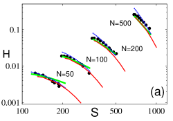
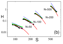
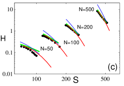
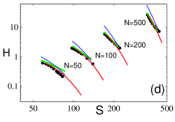
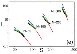
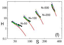
Figure 1: Rf heating rates of nonneutral plasmas in a Paul trap as a function of cloud size $S$ for $N=50$, 100, 200, and 500 particles and (a) $q=0.10$, (b) $q=0.15$, (c) $q=0.20$, (d) $q=0.25$, (e) $q=0.30$, (f) $q=0.35$. Plot symbols: Molecular-dynamics simulations. Heavy green line: Analytical, temperature-dependent rf-heating formula. Dashed blue line: Analytical rf heating formula with equi-partition approximation. Thin red line: Mean-field approximation.

In this section we present our numerical and analytical methods for evaluating the heating rate $H=H(S,N,q)$. The numerical results obtained in Section 3.1 provide the target data sets to be matched by our analytical formulas developed in Section 3.2. This succeeds to an excellent degree of accuracy. In Section 3.3, we compare the results of our molecular-dynamics simulations with the solutions of a nonlinear mean-field equation. Excellent agreement between the rf heating rates obtained by these two qualitatively different numerical methods is obtained. This provides an independent check of our molecular-dynamics simulations.

3.1 Molecular dynamics simulations

Using a 5th order Runge-Kutta method [18], we performed extensive molecular-dynamics simulations [19] of (1), extracting rf heating rates as discussed in [14] directly via computation of $dE/dt$ according to (4) for $N=50$, 100, 200, and 500 particles and $q=0.10$, 0.15, 0.20, 0.25, 0.30, and 0.35. The resulting rf heating rates are shown as a function of cloud size $S$ as the black data points in Fig. 1. While rf heating rates for $q=0.2$ were already computed and presented in [14], the data set displayed in Fig. 1, covering six different $q$ values, is more extensive than the data set presented in [14]. We checked that the rf heating rates in the $q=0.20$ panel of Fig. 1 are consistent with the rf heating rates presented in [14].

3.2 Analytical heating formulas

Defining the temperature

$$T=\frac{1}{3}\lim_{n\rightarrow\infty}\frac{1}{n}\sum_{k=1}^{n}\sum_{i=1}^{N}\dot{\vec{R}}_{i}^{2}(k\pi),$$ (6)

of a plasma cloud in the stationary state [15], the kinetic energy of the plasma cloud may be evaluated immediately on the basis of (2). The result is [15]

$$E_{\rm kin}=\frac{3N}{2}\left(1+\frac{q^{2}}{4}\right)T+\frac{1}{2}q^{2}S^{2},$$ (7)

where we assumed that the micro- and macromotions are uncorrelated. Since, in the stationary state, $\gamma$ determines the cloud size $S$, we may write $\gamma=\gamma(S,N,q)$. This way, if $\gamma(S,N,q)$ is known, we may use (4) and (7) to compute $H(S,N,q)$ analytically.

Our analytical formula for $\gamma(S,N,q)$ is based on the $q$ and $N$ scaling of the critical gamma, $\gamma_{c}(N,q)$, at which the transition to the crystal occurs [20]. In [20] we found that for a given $q$, $\gamma_{c}$ scales like an iterated-log law in $N$. In order to reveal the $q$ dependence of $\gamma_{c}$, we performed extensive additional molecular-dynamics simulations and established that

$$\gamma_{c}(N,q)=C(q)\ln[\ln(N)]-D(q),$$ (8)

where

$$C(q)=1.31\times q^{4.57},\ \ \ D(q)=0.13\times q^{3.77}.$$ (9)

Additional molecular-dynamics simulations then allowed us to determine the complete scaling of $\gamma(S,N,q)$. We found

$$\gamma(S,N,q)=\gamma_{c}(N,q)\exp\left[-2q^{0.9}\left(\frac{S-S_{c}(N,q)}{\sqrt{S_{c}(N,q)}}\right)\right],$$ (10)

where $S_{c}(N,q)$ is the critical cloud size (the smallest possible cloud size) at $\gamma=\gamma_{c}$. Since $S_{c}$ is very close to the size $S_{\rm crystal}(N,q)$ of the crystal, we write

$$S_{c}(N,q)=S_{\rm crystal}(N,q)+\sigma(N,q),$$ (11)

where [15]

$$S_{\rm crystal}(N,q)=\left(\frac{3}{5q^{4/3}}\right)^{1/2}N^{5/6}.$$ (12)

For the shift function $\sigma$ we found empirically that

$$\sigma(N,q)=[37.8\ln(N)-96.6]\exp\left\{-[1.4\ln(N)+3.1]q\right\}.$$ (13)

On the basis of the above formulas, $\gamma(S,N,q)$ can now be assembled and expressed in closed form as an analytical function.

The only missing ingredient for the use of (7) for the construction of an analytical representation of $H(S,N,q)$ is now a knowledge of $T(S,N,q)$. Based on our extensive numerical data sets we found

$$T(S,N,q)=0.7\left[\frac{\gamma(S,N,q)}{\gamma_{c}(N,q)}\right]^{-0.9},$$ (14)

which is valid for temperatures $0.7\lesssim T\lesssim 3$. Since, at this point, both $\gamma(S,N,q)$ and $\gamma_{c}(N,q)$ are known analytically, $T(S,N,q)$ is known analytically, which implies that $H(S,N,q)$ is now known analytically. We may also use (14) together with (10) to obtain $S$ as a function of $T$, $N$, and $q$ according to

$$S(T,N,q)=S_{c}(N,q)+\frac{\sqrt{S_{c}(N,q)}}{1.8\times q^{0.9}}\ln\left(\frac{T}{0.7}\right).$$ (15)

The heavy, green, solid lines in Fig. 1 represent $H(S,N,q)$ evaluated analytically in the range from $S_{c}(N,q)$ to $S(T=5,N,q)$ according to the formulas stated explicitly above. We see that for small $S$ (low temperature $T$) the analytical formula for $H(S,N,q)$ fits the numerical simulation data very well. The analytical lines start deviating from the numerical data for larger $S$ values, which we established to correspond to a temperature of $T\approx 3$. The deviation is due to our temperature formula (14), which is valid only for low temperatures close to the temperature where the cloud $\rightarrow$ crystal phase transition occurs [20]. Nevertheless, as seen in Fig. 1, the temperature range up to $T=3$ covers a considerable range in $S$.

For $T>3$ a different approach turned out to be useful. Assuming equipartition between the micromotion and the kinetic energy of the macromotion [21] turns (7) into

$$E_{\rm kin}=q^{2}S^{2}.$$ (16)

Using this expression for $E_{\rm kin}$ in (4) results in the dotted blue lines in Fig. 1. We see that for small temperatures the assumption (16) of equi-partition is not as good as using the temperature-dependent formula (7), but improves markedly for $T>3$. Therefore, we recommend to compute $H(S,N,q)$ on the basis of (7) for $T<3$ and on the basis of (16) for $T>3$. While, as documented in Fig. 1, this piecewise definition of our analytical formula for $H(S,N,q)$ works very well, we are currently working on an improved formula for $T(S,N,q)$, which will uniformly cover the entire range of $S$, $N$, and $q$ values.

3.3 Mean-field calculations

In order to check our numerical simulations, we solved the mean-field equation (55) in [15] for $T=0.7$, 1, 2, 3, 4, and 5, for each of the $q$-$N$ combinations shown in Fig. 1. The resulting heating rates are shown as the thin, red lines in Fig. 1. The excellent agreement between the mean-field calculations and our numerical molecular-dynamics simulations in the temperature range $0.7\leq T<5$ shows that (i) our molecular-dynamics simulations are reliable and (ii) detailed and expensive molecular-dynamics simulations in this temperature regime are not necessary; a much cheaper mean-field calculation suffices. Although our analytical heating formulas (solid, green and dashed, blue lines in Fig. 1) were computed over the same temperature range as our mean-field heating rates, Fig. 1 shows that the lines corresponding to our analytical results systematically terminate at smaller $S$ values than the mean-field heating rates (thin, red lines in Fig. 1). The reason is the following. For computing the end points $S(T=5,N,q)$ of the lines that represent our analytical results, we used the analytical formula (15). This formula, however, is based on our temperature formula (14), which, as mentioned above, is valid only for $T\lesssim 3$ and deteriorates for $T\gtrsim 3$. This results in a prediction of $S(T=5,N,q)$, which, typically, is of the order of 20% smaller than the $S$ value at $T=5$ predicted by our mean-field calculations. The log scale used in Fig. 1 exaggerates this relatively small difference.

4 Discussion

To our knowledge, our analytical rf heating formulas for $H(S,N,q)$ are the first such formulas that comprehensively cover the entire parameter range of rf-driven nonneutral plasmas stored in a hyperbolic Paul trap. This is significant, since $H(S,N,q)$, over the $S$, $N$, and $q$ ranges shown in Fig. 1, covers approximately 5 orders of magnitude.

We are well aware of the fact that our analytical heating formula is not derived from first principles. This would be an exceptionally difficult task to accomplish, which, to date, has not even succeeded in the case $N=2$. Yet, our analytical heating formula is much more than, say, a fit of a multi-variable polynomial to the results of our heating simulations. The difference is that the fit functions we use are not arbitrary, but carefully extracted from the $S$, $N$, and $q$ dependence exhibited by the heating rates provided by our molecular-dynamics simulations. Thus, only the numerical constants are fitted, while the shape of the fit functions is dictated by our data. Therefore, although our heating formula is based on input information of the rf heating of nonneutral plasmas for only up to $N=500$ particles, but since it is based on scaling properties extracted directly from the data, our analytical heating formula has predictive power and remains valid for $N\gg 500$. We spot-checked this explicitly by comparing rf heating rates computed via both molecular-dynamics simulations and our analytical rf heating formula for $q=0.2$ and $N=1,000$, $N=2,000$, and $N=5,000$ particles, which, currently, is the limit of our computer resources. However, using our vastly faster mean-field calculations, allowed us to check the validity of our analytical rf heating formula for several values of $q$ and particle numbers up to $N=10^{5}$.

Currently we are unable to extend our molecular-dynamics simulations with confidence beyond the $S$ values shown in Fig. 1. This has two reasons. (i) According to (10) the damping constant required to establish a stationary state for large $S$ is exponentially small, requiring exponentially long simulation times, which are currently beyond our computer budget. (ii) For exponentially small $\gamma$, the damping term in (1) is exponentially small compared with the other terms in (1) and is drowned out by numerical round-off noise. Keeping our current numerical methods, obtaining reliable numerical results for very small $\gamma$ can only be achieved by running our simulations in quadruple precision, which will extend the already exponentially long simulation times as discussed in (i). Nevertheless, exploring the large-$S$, large-$T$ regime is definitely on our agenda.

While the small-$S$ regime, explored in this Letter, allows for a relatively simple, unified treatment in terms of particle dynamics and heating rates, the large-$S$ regime, currently inaccessible to our numerical simulation methods, may hold surprises. For increasing $T$, the plasma becomes increasingly more dilute; a tenuous, one-component, nonneutral plasma results, in which single-particle properties may dominate collective plasma properties. The result is a much richer, nonlinear dynamics, which may be impossible to capture with a single, analytical heating formula $H(S,N,q)$ with a simple closed-form analytical structure as presented in this Letter in the small-$S$, low-temperature regime.

In this Letter we focused our discussion on the energy flow from the rf field to the trapped nonneutral plasma in the stationary state, established in the presence of a damping mechanism, modelled in (4) in terms of a damping term with damping constant $\gamma$. This is a situation we called situation (A) in Section 1. In this case, in addition to providing power to heat up the trapped plasma, the rf field has to provide power to sustain the micromotion in the presence of damping. The power necessary to sustain the micromotion is $\gamma q^{2}S^{2}/2$. In situation (B), no damping is present, and $\gamma$ is zero. In this situation all the power provided by the rf field is used to heat up the plasma; providing power for sustaining the micromotion is not necessary in situation (B). Therefore, the plasma heating rate $H_{P}(S,N,q)$ may be obtained from the heating rate $H(S,N,q)$, pertaining to situation (A), via

$$H_{P}(S,N,q)=H(S,N,q)-\frac{1}{2}\gamma(S,N,q)q^{2}S^{2},$$ (17)

where $\gamma(S,N,q)$ is the damping constant necessary to achieve the stationary state with cloud size $S$. We verified the validity of (17) explicitly via molecular-dynamics simulations in which we first established the stationary state with the help of $\gamma(S,N,q)$, subsequently taking $\gamma$ to zero in (1), and then evaluating $H_{P}(S,N,q)$ during the $\gamma=0$ expansion phase of the cloud.

In this Letter we restricted ourselves to the discussion of spherical plasma clouds, i.e., $a=q^{2}/2$. We are currently working on extending our results to the case of non-spherical plasma clouds in the hyperbolic Paul trap, and to the case of plasma clouds in the linear Paul trap [4, 5, 6]. No new analytical or numerical tools have to be developed since the conceptual framework established in this Letter is applicable to all rf-trap architectures.

5 Summary, conclusions, and outlook

In this Letter we present, for the first time, a comprehensive, explicit, analytical heating formula that allows us to compute rf heating rates in the form $H(S,N,q)$ [$H_{P}(S,N,q)$, respectively] for all trapped, spherical, nonneutral plasmas in a hyperbolic Paul trap in the low-temperature regime. Our formula, defined piecewise in two branches ($T<3$ and $T>3$), shows excellent agreement with detailed microscopic, time-dependent molecular-dynamics calculations and time-independent mean-field simulations conducted in the low-temperature regime ($T<5$). Our analytical and numerical methods define a general framework that may be applied to the construction of rf heating formulas for all rf-trap architectures and cloud shapes.

6 Acknowledgment

YSN acknowledges support from ARO MURI award W911NF-16-1-0349.

Appendix: Conversion to SI units

Dimensionless quantities, as used in the main body of this paper, are the most convenient choice if the general, universal features of a given system are emphasized. However, if used for practical applications and laboratory experiments, SI units are more convenient.

If the trapped nonneutral plasma consists of particles of charge $Q$ and mass $m$, the control parameters $a$ and $q$ are given by [13]

$$a=\frac{8QU_{0}}{m\Omega^{2}(r_{0}^{2}+2z_{0}^{2})},\ \ \ q=\frac{4QV_{0}}{m\Omega^{2}(r_{0}^{2}+2z_{0}^{2})},$$ (18)

where $r_{0}$ and $z_{0}$ are the distances of the Paul trap’s ring electrode and end-cap electrodes from the center of the trap, respectively, $U_{0}$ and $V_{0}$ are the dc and ac voltages applied to the trap, respectively, $\Omega=2\pi f$ is the angular frequency of the trap, and $f$ is the ac frequency of the trap in Hz. With these quantities, the unit of time is

$$t_{0}=\frac{2}{\Omega},$$ (19)

the unit of length is

$$l_{0}=\left(\frac{Q^{2}}{\pi\epsilon_{0}m\Omega^{2}}\right)^{1/3},$$ (20)

the unit of energy is

$$E_{0}=\frac{ml_{0}^{2}}{t_{0}^{2}},$$ (21)

the unit of temperature is

$$T_{0}=\frac{E_{0}}{k_{B}},$$ (22)

where $k_{B}$ is Boltzmann’s constant, and the unit of heating rate is

$$H_{0}=\frac{E_{0}}{t_{0}}=\frac{ml_{0}^{2}}{t_{0}^{3}}.$$ (23)

Thus, the heating rate $H^{(SI)}$ in SI units is computed from the dimensionless heating rate $H$ according to

$$H^{(SI)}(S,N,q)=H_{0}\,H(S,N,q),$$ (24)

and the temperature $T^{(SI)}$ in SI units is computed from the dimensionless temperature $T$ according to

$$T^{(SI)}(S,N,q)=T_{0}\,T(S,N,q).$$ (25)

References

References

- [1] W. Paul, Rev. Mod. Phys. 62, 531 (1990).
- [2] P. K. Ghosh, Ion Traps (Clarendon Press, Oxford, 1995).
- [3] C. W. Chou, D. B. Hume, J. C. J. Koelemeij, D. J. Wineland, and T. Rosenband, Phys. Rev. Lett. 104, 070802 (2010).
- [4] T. P. Harty, D. T. C. Allcock, C. J. Ballance, L. Guidoni, H. A. Janacek, N. M. Linke, D. N. Stacey, and D. M. Lucas, Phys. Rev. Lett. 113, 220501 (2014).
- [5] A. C. Wilson, Y. Colombe, K. R. Brown, E. Knill, D. Leibfried, and D. J. Wineland, Nature (London) 512, 57 (2014).
- [6] S. Debnath, N. M. Linke, C. Figgatt, K. A. Landsman, K. Wright, and C. Monroe, Nature (London), 536, 63(2016).
- [7] H. C. Chang, Ann. Rev. Anal. Chem. 2, 169 (2009).
- [8] T. Pruttivarasin, M. Ramm, S. G. Porsev, I. I. Tupitsyn, M. S. Safronova, M. A. Hohensee, and H. Häffner, Nature (London) 517, 592 (2015).
- [9] R. F. Wuerker, H. Shelton, and R. V. Langmuir, J. Appl. Phys. 30, 342 (1959).
- [10] H. G. Dehmelt, Adv. At. Mol. Phys. 3, 53 (1967); 5, 109 (1969).
- [11] R. Blatt, P. Gill, and R. C. Thompson, J. Mod. Opt. 39, 193 (1992).
- [12] R. Blümel, J. M. Chen, E. Peik, W. Quint, W. Schleich, Y. R. Shen and H. Walther, Nature 334, 309 (1988).
- [13] R. Blümel, C. Kappler, W. Quint and H. Walther, Chaos and Order of Laser Cooled Ions in a Paul-Trap, Phys. Rev. A40, 808 (1989).
- [14] J. D. Tarnas, Y. S. Nam and R. Blümel, Phys. Rev. A 88, 041401(R) (2013).
- [15] Y. S. Nam, E. B. Jones, and R. Blümel, Phys. Rev. A 90, 013402 (2014).
- [16] R. C. Davidson, Theory of Nonneutral Plasmas (W. A. Benjamin, London, 1974).
- [17] M. D. N. Lunney, F. Buchinger, and R. B. Moore, Journal of Modern Optics 39, 349 (1992).
- [18] W. H. Press, S. A. Teukolsky, W. T. Vetterling, and B. P. Flannery, FORTRAN Numerical Recipes, 2nd ed. (Cambridge University Press, Cambridge, 1992).
- [19] J. M. Haile, Molecular Dynamics Simulation (John Wiley & Sons, NY, 1997).
- [20] D. K. Weiss, Y. S. Nam, and R. Blümel, Phys. Rev. A 93, 043424 (2016).
- [21] T. Baba and I. Waki, Appl. Phys. B 74, 375 (2002).