Self-exciting point processes with spatial covariates: modeling the dynamics of crime

Abstract

Crime has both varying patterns in space, related to features of the environment, economy, and policing, and patterns in time arising from criminal behavior, such as retaliation. Serious crimes may also be presaged by minor crimes of disorder. We demonstrate that these spatial and temporal patterns are generally confounded, requiring analyses to take both into account, and propose a spatio-temporal self-exciting point process model that incorporates spatial features, near-repeat and retaliation effects, and triggering. We develop inference methods and diagnostic tools, such as residual maps, for this model, and through extensive simulation and crime data obtained from Pittsburgh, Pennsylvania, demonstrate its properties and usefulness.

1 Introduction

As police departments have moved to centralized computer databases of crime reports, models to predict the risk of future crime across space and time have become widely used. Police departments have used predictive methods to target interventions aimed at reducing property crime (Hunt et al., 2014; Mohler et al., 2015) and violent crime (Ratcliffe et al., 2011; Taylor et al., 2011), and to analyze hotspots of robbery (Van Patten et al., 2009) and shootings (Kennedy et al., 2010), among many other applications. Predictive policing methods are now widely deployed, with law enforcement agencies routinely making operational decisions based on them (Perry et al., 2013), and meta-analyses have shown that these policing programs can result in statistically significant crime decreases (Braga et al., 2014).

Predictive models of crime come in several forms. The most common are tools to identify “hotspots,” small regions with elevated crime rates, using methods like kernel density estimation or hierarchical clustering on the locations of individual crimes (Levine, 2015). These tools produce static hotspot maps that can be used to direct police patrols. A substantial research literature demonstrates that crime is highly clustered, justifying hotspot methods that identify clusters for intervention (Braga et al., 2014; Andresen et al., 2017), though these methods typically do not model changes in hotspots over time, even though research suggests that some hotspots emerge and disappear over weeks or months (Gorr and Lee, 2015).

Other analysis focuses on “near-repeats”: a locally elevated risk of crime immediately after a location experiences a crime, with the risk decaying back to the baseline level over a period of weeks or months. Near-repeats are often analyzed using methods borrowed from epidemiology that assess space-time clustering, such as Knox tests (Ratcliffe and Rengert, 2008; Haberman and Ratcliffe, 2012), though these methods are not very fine-grained, giving only a sense of the distance and time over which near-repeat effects are statistically significant but not the form of their decay or uncertainty in their effect. Nonetheless, near-repeat behavior has been observed for burglaries, possibly because burglars return to areas with which they are familiar (Townsley et al., 2003; Bernasco et al., 2015), and also with other types of crime, perhaps connected to gang activities and retaliation attacks (Youstin et al., 2011).

A range of regression-based analyses are also used to predict crime risks. One approach uses the incidence of “leading indicator” offenses as covariates to predict more serious crimes at later times, and taking leading indicators into account can improve predictions of crime (Cohen et al., 2007; Gorr, 2009). Leading indicators include various minor crimes, such as criminal mischief or liquor law violations, and police agencies can target intervention if they know which leading indicators predict which types of crime. On a larger scale, the “broken windows” theory states that low-level offenses, if not adequately controlled, lead to more serious crimes as social control disintegrates (Kelling and Wilson, 1982). Research on the broken windows hypothesis has had mixed results, suggesting the need for further tests of its predictive power (Harcourt and Ludwig, 2006; Cerdá et al., 2009).

Finally, regression is also used to assess local risk factors for crime. Risk Terrain Modeling (Kennedy et al., 2010, 2016) divides the city into a grid, regressing the number of crimes recorded in each grid cell against the presence of selected risk factors, such as gang territories, bars, high-risk housing complexes, recent parolees, and so on. The regression output gives police a quantitative assessment of the “risk terrain”, and enables directed interventions targeted at specific risk factors, which can more efficiently use police resources to reduce crime. The identification of risk factors is also important for developing criminological theory to understand the nature and causes of crime (Brantingham and Brantingham, 1981).

Together, these lines of research show the range of statistical methods used to answer important policing policy questions using historical crime data. In this paper, we introduce a single self-exciting point process model of crime that unifies features of all of these methods, accounting for near-repeats, leading indicators, and spatial risk factors in a single model, and producing dynamic hotspot maps that account for change over time. We develop a range of diagnostic and simulation tools for this model. Furthermore, we demonstrate a serious flaw in previous statistical methods: if leading indicators, near-repeats, and spatial features are not modeled jointly, their effects are generically confounded. This confounding may have affected previously published results. Additional simulations illustrate confounding issues that remain when some covariates are unmeasured or unknown, making it inherently difficult to interpret any spatio-temporal model.

The point process model of crime proposed here extends a model introduced by Mohler et al. (2011) and refined by Mohler (2014). This model accounts for changing hotspots and near-repeats by assuming that every crime induces a locally higher risk of crime that decays exponentially in time; hotspots, where many crimes occur in a short period of time, decay away unless sustained criminal activity keeps the crime intensity high. In addition, the model includes a fixed background to account for chronic hotspots, and allows leading indicator crimes to contribute to the crime intensity, with weights varying by crime type and fit by maximum likelihood. Mohler et al. (2015) demonstrated that a simplified version of this model, used to assign daily patrol priorities for a large urban police department, can beat predictions by experienced crime analysts, leading to a roughly 7.4% reduction in targeted crimes.

We extend the model proposed by Mohler (2014) to incorporate spatial features, enabling tests of criminological theory; by introducing parameter inference tools, allowing quantification of near-repeats and tests of leading indicator parameters; and with residual analysis methods, providing fine-grained analysis of model fit. The utility of the model is then demonstrated on a large dataset of crime from Pittsburgh, Pennsylvania. We begin by considering the confounding factors that make a full spatio-temporal model necessary.

2 Heterogeneity and state dependence

The risk of crime varies in space and time both because of spatial heterogeneity—local risk factors for crime, differing socioeconomic status, zoning, property development, policing patterns, local businesses, and so on—and through dependence on recent state, such as recent crimes that may trigger retaliation or signal the presence of a repeat offender. In the criminological literature, these effects have often been studied separately, but this is problematic. A long line of research suggests that, in general, the effects of heterogeneity and state dependence are difficult to distinguish in observational data and can be confounded (Heckman, 1991). We investigate this possibility in this section, demonstrating the need for crime models that control for both effects.

Spatial heterogeneity is usually studied with tools like Risk Terrain Modeling (Kennedy et al., 2010, 2016), discussed above. At the same time, a separate line of research has focused on near-repeat and flare-up effects, which cause short, local bursts of crime activity, with high risks stimulated by recent criminal activity. Some crimes may occur not because of features of the local environment but in response to recent crimes in the same area. As Johnson (2008) pointed out, however, these two effects may be confounded. If a particular neighborhood is “flagged”—that is, has a risk factor that makes it more attractive to criminals—it will experience a higher rate of crime, and after any particular crime, the local risk of a repeat offense will appear to be higher than in other parts of the city without the risk factor. But this is because of the local risk factor, not because the occurrence of one crime “boosted” the risk temporarily. Boosting and flagging are two substantively different causal theories of crime, and suggest different policies and interventions to address their causes, but may be difficult to distinguish from recorded crime data alone.

To distinguish between these causes, Johnson (2008) proposed a simulation approach. A virtual set of households was created, each with a baseline risk of burglary that depended on separate risk factors, and in each interval of time, burglaries were simulated based on the risk factors. Separate simulations were run with and without a boosting effect. Repeated across many simulations, this produced patterns of near-repeats that could be compared against observed crime data, and it was found that the simulations containing the boost effect matched the observed data much better than those without. Short et al. (2009), in a similar approach, specified several different stochastic models of crime, and found that a model incorporating near-repeat behavior fit the observed distribution of burglaries in Los Angeles much better than one without.

However, the ability to distinguish specific models or simulations does not imply that the two effects are not confounded in general. Fig. 1 gives a simplified causal diagram (Pearl, 2009) of near-repeat behavior in one particular grid cell $i$. The past occurrence of crime at time $t-1$ may influence the rate of crime at $t$ (the boost effect), shown by an arrow between the two, as may two separate risk factors, which affect the occurrence of crime at both time points (the flagging effect). Crucially, if the boost effect is ignored, the flagging effect of the covariates at time $t$ is confounded, and vice versa. It may be possible in specific simulations or in specific stochastic models to distinguish situations with boosting from those without, but in general, estimates of the size of each effect will be confounded; to understand spatial risk factors we must account for the boosting, and to understand boosting we must account for the spatial risk factors.

Figure 1: A simplified causal diagram of crime observed in a grid cell $i$ at two times, $t$ and $t-1$, when there are two covariates that may affect the rate of crime.

A simple simulation can demonstrate this effect. Using the model to be introduced in Section 3.1, we simulate crimes occurring on a grid with two spatially-varying risk factors for crime, along with a near-repeat effect. This effect is controlled by a parameter $\theta$, which specifies the average number of crimes triggered by each occurring crime. We then perform a spatial Poisson regression, counting the simulated crimes that occurred in each grid cell and regressing against the simulated risk factors. The coefficients $\beta$ for the intercept and risk factors are shown in Fig. 2, for simulations ranging from no near-repeat behavior ($\theta=0$) to a great deal of near-repeats ($\theta\approx 1$). As near-repeats increase, regression coefficients gradually get more biased. The intercept, $\beta_{0}$, increases to account for the additional crimes; the covariate coefficient $\beta_{1}$ decreases from its true value of $4.8$, and $\beta_{2}$ increases from its true value of $-2.3$. Notably, both covariate coefficients shrink towards zero in the presence of near repeats, and the magnitude of this effect is large compared to their absolute size.

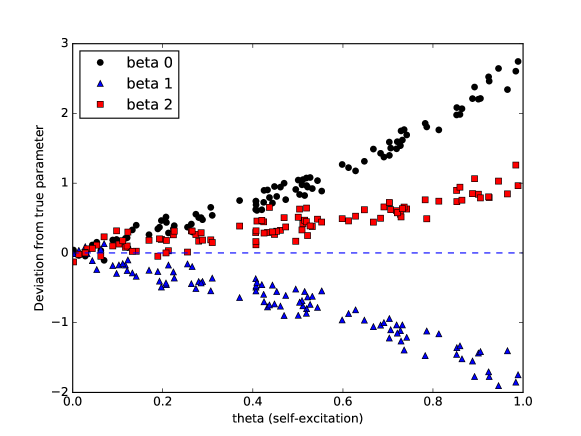
Figure 2: As the near-repeat effect increases from 0 crimes triggered to 1 crime triggered for every observed crime, spatial Poisson regression coefficients gradually become more and more biased.

In certain circumstances, using spatial risk factors with particular patterns, near-repeats can cause false positives: risk factors that appear related to crime rates but are not. For example, Fig. 3 shows two synthetic spatial covariates. One is nonzero in a center square, the other in a ring around that square. Only the first covariate has a true nonzero coefficient, but because the near-repeat effect produces crimes slightly outside the square, its effect “leaks” to the outer ring, causing the second covariate to appear to have a positive coefficient, as shown in the simulation results in Fig. 4.

Figure 3: Two synthetic covariates. The covariates have value 1 in the white areas and zero elsewhere. The covariate on the left has a true coefficient of zero in the simulations, while the covariate on the right has a positive true effect. The spatial decay distance is $\sigma=5$ pixels, so the effect of the right covariate spreads to the area of the left covariate.

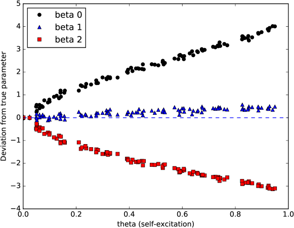
Figure 4: As the amount of self-excitation increases, the coefficient $\beta_{1}$ (the left covariate in Fig. 3) increases from zero, despite its true value being zero. $\beta_{2}$ shrinks toward zero for the same reason as in Fig. 2.

It is hence clear that methods to estimate spatial risk factors must take into account near repeats or suffer bias and potentially false positives in their estimated coefficients. In Section 4.3, further simulations using the model to be developed below will show the opposite effect: unaccounted-for spatial risk factors bias estimates of the rate of near repeats, potentially resulting in estimates that overestimate the boost effect. To resolve these problems, we propose a self-exciting point process model for crime that can account for both near repeats and spatial risk factors simultaneously, eliminating the confounding.

3 Methods

3.1 Self-exciting point process model

Self-exciting point process models are a class of models for spatio-temporal point process data that incorporate “self-excitation”: each event may excite further events, by locally increasing the event rate for some period of time. This corresponds to the near repeat phenomenon we need to account for. Self-exciting point processes are a development of Hawkes processes (Hawkes, 1971), which are purely temporal processes. The theory and applications of self-exciting spatio-temporal point processes were reviewed by Reinhart (2018); we give only a brief summary here.

A spatio-temporal point process is characterized by its conditional intensity function, defined for locations $s\in X\subseteq\operatorname{\mathbb{R}}^{d}$ and times $t\in[0,T)$ as

$$\lambda(s,t\mid{\cal H}_{t})=\lim_{\Delta s,\Delta t\downarrow 0}\frac{\operatorname{\mathbb{E}}\left[N\left(B(s,\Delta s)\times[t,t+\Delta t)\right)\mid{\cal H}_{t}\right]}{|B(s,\Delta s)|\Delta t},$$ (1)

where $|B(s,\Delta s)|$ is the Lebesgue measure of the ball $B(s,\Delta s)$ with radius $\Delta s$, $N(A)$ is the counting measure of events over the set $A\subseteq X\times[0,T)$, and ${\cal H}_{t}$ is the history of events in the process up to time $t$. In the limit, the conditional intensity can be interpreted as the instantaneous rate of events per unit time and area, and hence the expected number of events in time interval $[t_{1},t_{2})$ and region $B$ is

$$\operatorname{\mathbb{E}}[N(B\times[t_{1},t_{2}))]=\int_{t_{1}}^{t_{2}}\int_{B}\lambda(s,t)\operatorname{d\!}s\operatorname{d\!}t.$$

Self-exciting point processes have conditional intensities of the form

$$\lambda(s,t\mid{\cal H}_{t}) =\mu(s)+\sum_{i\mathrel{\mathop{\mathchar 58\relax}}t_{i}<t}g(s-s_{i},t-t_{i})$$

$$=\mu(s)+\int_{0}^{t}\int_{X}g(s-u,t-r)\operatorname{d\!}N(u\times r),$$

where $g$ is a triggering function that determines the form of the self-excitation. In the remainder of this paper, we will refer to $\lambda(s,t)$ without the explicit ${\cal H}_{t}$ to simplify notation, but $\lambda(s,t)$ should still be understood to depend on the past history of the process.

Models of this form have been widely used in a variety of processes exhibiting clustering, such as earthquake epicenters (Ogata, 1999) and the occurrence of infectious diseases (Meyer et al., 2012; Meyer and Held, 2014). Mohler et al. (2011) developed such a model for the occurrence of violent crime by building on the models used in earthquake forecasting, known in the seismology literature as epidemic-type aftershock sequence models (Ogata, 1999). This model allows hotspot estimates to change over time by separating crime into chronic hotspots, which remain fixed in time, and temporary hotspots, which are caused by increases or changes in crime. (In seismological models, earthquakes are similarly divided into main shocks and aftershocks triggered by those main shocks.) Hotspot intensities are modeled with a modification of kernel density smoothing, where past crimes contribute to the intensity with effects that decay away in time, and the bandwidth parameters are estimated to best fit the data instead of being chosen by the operator.

Mohler (2014) further adapted the model to include leading indicator crimes, producing a model that predicts the conditional intensity $\lambda(s,t)$ of crime at each location $s$ and time $t$ as the sum of a background rate and a sum of functions of prior crimes:

$$\lambda(s,t)=\mu(s)+\sum_{\begin{subarray}{c}\text{all events }i\\ \text{ before time }t\end{subarray}}g(s-s_{i},t-t_{i},M_{i}),$$ (2)

where $\mu(s)$ is a background crime rate that does not vary in time, and $s_{i}$ and $t_{i}$ are locations and times of other crimes used as leading indicators. $M_{i}$ represents the type of each leading indicator crime, as different indicators are allowed to have different predictive effects in this model.

The triggering function $g$ is defined to be

$$g(s,t,M)=\frac{\theta_{M}\omega}{2\pi\sigma^{2}}\exp(-\omega t)\exp\left(-\frac{\|s\|^{2}}{2\sigma^{2}}\right),$$

where $\sigma^{2}$ is the bandwidth, $\theta_{M}$ determines how much each type of leading indicator contributes to the intensity, and the effect decays exponentially in time with a rate controlled by $\omega$. Because $g$ is chosen to integrate to $\theta_{M}$, it has a natural interpretation: the expected number of target crimes induced by a single leading indicator crime of type $M$.

Mohler (2014) chose the background crime rate $\mu(s)$ to be a sum of weighted Gaussian kernels centered at prior crimes:

$$\mu(s)=\sum_{i}\frac{\alpha_{M_{i}}}{2\pi\eta^{2}T}\exp\left(-\frac{\|s\|^{2}}{2\eta^{2}}\right).$$ (3)

Here $\alpha_{M_{i}}$ determines the contribution of each leading indicator type to the background rate, $\eta^{2}$ is the bandwidth, and $T$ is the total length of time over which the crime data falls.

This model has several limitations. The background component (3) does not explicitly account for varying spatial features or give estimates of their effects, and the use of weighted Gaussian kernels for both $g(s,t,M)$ and $\mu(s)$ makes the model parameters difficult to identify; to prevent multiple modes in the log-likelihood, Mohler (2014) had to set $\sigma=\eta$.

We have extended this model to replace the nonparametric $\mu(s)$ with one that directly incorporates spatial covariate information, allowing estimates of the effects of each covariate and avoiding identifiability issues. We assume that the observation domain $X$ is divided into cells $c$ of arbitrary shape, inside of which a covariate vector $X_{c}$ (including an intercept term) is known, resulting in the model

$$\lambda(s,t)=\exp\left(\beta X_{C(s)}\right)+\sum_{i\mathrel{\mathop{\mathchar 58\relax}}t_{i}<t}g(s-s_{i},t-t_{i},M_{i}),$$ (4)

where $C(s)$ is the index of the covariate cell containing $s$ and the triggering function $g$ is unchanged. We let $g(s,t,M)=0$ for $s<\delta$, for an arbitrary short distance $\delta$, to prevent crimes that occur at exactly the same location from enticing the model to converge to $\sigma=0$.

In principle, this model could be built with covariates that vary continuously in space, defined by a function $X(s)$. This would increase the generality of the model. However, in practice, this generality is not necessary: most socioeconomic, demographic, or land use variables are observed only in cells such as city blocks, census blocks, or neighborhoods. Piecewise constant covariates also make estimation and simulation more computationally tractable, and so the small loss in generality is worth the substantial gain in practicality.

We may also reasonably ask about the form of the triggering function $g$, which specifies an exponential decay in time and a Gaussian kernel in space. Meyer and Held (2014), for example, analyzing the spread of infectious disease, proposed a power law kernel to account for long-range flows of people. Unfortunately, most alternate spatial kernels make the expectation maximization strategy described below more difficult, by making analytical maximization on each iteration impossible. These kernels could still be used, but with the additional computational cost of numerical maximization.

3.2 Simulation algorithm

Simulations from self-exciting point process models have proved useful both for examining inference and for the simulation studies discussed in Sections 2 and 4. Various simulation algorithms for self-exciting point processes were discussed by Reinhart (2018, Section 3.3). We chose to use an algorithm introduced by Zhuang et al. (2004) for earthquake aftershock sequence models, which is fast and efficient for our model structure. This algorithm draws on a key property of self-exciting point processes shown by Hawkes and Oakes (1974): a self-exciting process can be represented as a cluster process. Cluster centers come from an inhomogeneous Poisson process with rate $\mu(s)$, and each cluster center produces a cluster of offspring events with locations and times determined by the triggering function $g(s,t,M)$. Each of these offspring events may trigger further offspring of its own, and so on.

This leads to a natural simulation procedure that first draws from the inhomogeneous Poisson cluster center process, then draws a generation of offspring based on those cluster centers, and repeats until there are no more offspring. Full details are given by Zhuang et al. (2004). Draws from the cluster center process are made easier by our assumption that the observation domain is divided into cells $c$, inside each of which is a constant covariate vector $X_{c}$; we can hence draw cluster centers from homogeneous Poisson processes inside each cell.

Our simulation system can simulate from the model specified by eq. (4), but can also simulate various violations of assumptions: the spatial distribution of offspring can be Gaussian, $t$ with arbitrary degrees of freedom, Cauchy, or various other shapes, and their temporal distribution can be drawn from an exponential distribution or a Gamma distribution with arbitrary parameters. The framework is flexible and allows additional distributions to be chosen easily; this feature will be used in Section 4.2 to test model performance under various types of misspecification.

3.3 Parameter inference

Mohler (2014) fit the self-exciting model by maximum likelihood, using the log-likelihood function for spatio-temporal point processes:

$$\ell(\Theta)=\sum_{i}\log\lambda(s_{i},t_{i})-\int_{0}^{T}\int_{X}\lambda(s,t)\operatorname{d\!}s\operatorname{d\!}t,$$ (5)

where $X$ is the spatial domain of the observations and $\Theta$ a complete vector of parameters. The log-likelihood is optimized via expectation maximization, using the approximation that $X=\operatorname{\mathbb{R}}^{2}$ to simplify calculation of the triple integral, which is valid when most crime triggered by the observed crimes occurs within the study area (Schoenberg, 2013). Note that, as the model predicts the target crime and not the leading indicators, only the target crimes are included in the sum in Eq. (5). We adapted the expectation maximization procedure to fit our extended model.

The expectation maximization procedure for self-exciting processes was first described by Veen and Schoenberg (2008), and follows the general procedure described by Reinhart (2018, Section 3.1). A latent variable $u_{i}$ is introduced for each event $i$, indicating whether the event came from the background process ($u_{i}=0$) or was triggered by a previous event $j$ ($u_{i}=j$). Augmented with this variable, the log-likelihood simplifies from the form in (5), since the intensity $\lambda(s_{i},t_{i})$ no longer involves a sum over the background $\mu(s)$ and all previous events but only the term indicated by $u_{i}$. We can then take the expectation and maximize. In our model, maximization proceeds in closed form for most parameters, apart from $\beta$, which must be separately numerically maximized on each iteration.

Mohler (2014) did not provide inference for the self-exciting point process model parameters, though they may be of interest: the self-excitation parameters $\sigma^{2}$, $\omega$, and $\theta$ may be used to test hypotheses about the concentration of crime and the nature of leading indicators. Mohler’s nonparametric background (3) also does not incorporate spatial covariates, though $\beta$ in our background indicates the association between spatial covariates and crime. There are several potential routes to deriving asymptotic confidence intervals for these parameters, which we consider in turn.

First, Rathbun (1996) demonstrated the asymptotic normality and consistency of the maximum likelihood estimator for spatiotemporal point processes: $\sqrt{T}(\hat{\Theta}-\Theta)\rightsquigarrow_{u}N(0,\Sigma)$ as $T\to\infty$, where $\rightsquigarrow_{u}$ represents uniform convergence in distribution and $\Theta$ is the complete vector of parameters. The result holds under certain regularity conditions on the conditional intensity. Rathbun (1996) suggested an estimator for the covariance matrix $\hat{\Sigma}$ of the parameter estimate $\hat{\Theta}$,

$$\hat{V}(\hat{\Theta})=\left(\sum_{i=1}^{N_{c}}\frac{\Delta(s_{i},t_{i})}{\lambda(s_{i},t_{i})}\right)^{-1},$$

where $\Delta(s,t)$ is a matrix-valued function with elements

$$\Delta_{ij}(s,t)=\frac{\dfrac{\partial{}}{\partial{\hat{\Theta}_{i}}}\lambda(s,t)\dfrac{\partial{}}{\partial{\hat{\Theta}_{j}}}\lambda(s,t)}{\lambda(s,t)}.$$ (6)

With the full estimated covariance matrix, we calculated standard errors for each estimator, and produced confidence intervals from these.

An alternate approach, following again from the asymptotic normality result, is to use the observed information matrix at the maximum likelihood estimate, based on the Hessian of the log-likelihood:

$$\hat{\Sigma}=-H(\hat{\Theta})^{-1},$$

where $H(\hat{\Theta})$ is the matrix of second partial derivatives of $\ell(\Theta)$ evaluated at $\hat{\Theta}$. This approach was suggested by Ogata (1978) in the context of an asymptotic normality result for temporal point processes, and has been frequently used for spatio-temporal models in seismology; however, Wang et al. (2010), comparing its estimated standard errors with those found by repeated simulation, found that it can be heavily biased for smaller samples.

Nonetheless, we implemented the estimator using Theano (Bergstra et al., 2010), a Python package for describing computations that automatically generates fast C code and automatically computes all necessary derivatives. We then performed a series of 350 simulations to compare the finite-sample performance of both estimators with our model, using randomly chosen parameter values, obtaining the results shown in Table 1. Coverage is worst for the self-excitation parameters $\sigma^{2}$, $\omega$, and $\theta$, which are affected by any remaining boundary effect (see Section 4.1) not compensated for by the buffer region; Rathbun’s covariance estimator achieves nearly nominal coverage for $\beta$, which is less affected. Overall, Rathbun’s estimator achieves 88% coverage and is closest to its nominal 95% coverage. We will use this estimator in our analysis in Section 5.

Table 1: Coverage of nominal 95% CIs

Variable	Hessian (%)	Rathbun (%)
$\sigma^{2}$	86	88
$\omega$	87	91
$\theta$	82	63
$\beta_{0}$	77	83
$\beta_{1}$	89	92
$\beta_{2}$	86	89
Average	85	88

3.4 Residual analysis

Once a model is fit, it is useful to be able to determine where the model fits: what types of systematic deviations are present, where covariates may be lacking, what types of crimes are over- or under-predicted, and so on. Eq. (1) suggests we can produce these detailed analyses: because the point process model predicts a conditional intensity at each location, we can calculate the expected number of crimes within each region in a certain period of time, and compare this against the true occurrences over the same time, producing a residual map. These residuals are defined to be (Daley and Vere-Jones, 2008, chapter 15)

$$R(h)=\int_{\operatorname{\mathbb{R}}\times\operatorname{\mathbb{R}}^{2}}h(s,t)\left[N(\operatorname{d\!}s\times\operatorname{d\!}t)-\lambda(s,t)\operatorname{d\!}t\operatorname{d\!}s\right],$$

where $N(\cdot)$ is the counting measure of events in the given region, and $h(s,t)$ is a bounded window function. Typically, $h(s,t)$ is taken to be an indicator function for a chosen spatio-temporal region.

To calculate $R(h)$, a typical approach is to choose a time window $[t_{1},t_{2})$—say, a particular week or month—and integrate the conditional intensity over this window, producing an integrated intensity function

$$\lambda(s)=\int_{t_{1}}^{t_{2}}\lambda(s,t)\operatorname{d\!}t.$$

Then the spatial region $X$ is divided appropriately and the intensity is integrated over each subdivision, then compared against the number of events in that subdivision during that time window.

Choosing spatial subdivisions for residuals requires care. The obvious choice is a discrete grid, but the right size is elusive: small grid cells produce skewed residuals with high variance (as most cells have no crimes), and positive and negative residual values can cancel each other out in large cells. Bray et al. (2014) instead suggest instead using the Voronoi tessellation of the plane, which produces a set of convex polygons, known as Voronoi cells, each of which contains exactly one crime and all locations that are closer to that crime than to any other.

Given this tessellation, the raw Voronoi residuals $\hat{r}_{i}$ for each cell $C_{i}$ are

$$\hat{r}_{i}=1-\int_{C_{i}}\hat{\lambda}(s)\operatorname{d\!}s.$$

The choice of Voronoi cells ensures that cell sizes adapt to the distribution of the data, and Bray et al. (2014) cite extensive simulations by Tanemura (2003) indicating that the Voronoi residuals of a homogeneous Poisson process have an approximate distribution given by

$$\hat{r}_{i}\sim 1-X,\qquad\text{where }X\sim\text{Gamma}(3.569,3.569),$$

so that $\operatorname{\mathbb{E}}[\hat{r}_{i}]=0$. (Here the gamma distribution is parametrized by its shape and rate.) But because the conditional intensity function (4) is not homogeneous, we performed similar simulations for random parameter values, fitting to 1,332,546 simulated residuals by maximum likelihood the approximate distribution $X\sim\text{Gamma}(3.389,3.400)$.

After each $\hat{r}_{i}$ is found, using Monte Carlo integration over $C_{i}$, the Voronoi cells can be mapped with colors corresponding to their residual values. To ease interpretation, colors are determined by $-\Phi^{-1}(F(1-\hat{r}_{i}))$ where $F$ is the cumulative distribution function of the approximate distribution of $X$ and $\Phi^{-1}$ the inverse normal cdf. Positive residuals hence indicate more observed crime than was predicted, and negative residuals less.

These residual maps provide much more detailed information than previous global measures of hotspot fit, and can indicate areas with unusual patterns of criminal activity. For example, consider a model that predicts homicides using leading indicators such as assault and robbery; this model may perform well in an area that experiences gang-related violence, but would systematically over-predict homicides in a commercial area full of bars and nightclubs, where most assaults are drunken arguments rather than signs of gang conflict. An example residual map is given in Fig. 12 (Section 5.2) for Pittsburgh burglary data, illustrating the use of this method.

The example map does illustrate one weakness of Voronoi residual maps. We would expect areas with large positive residuals (red, in the map) to have a higher crime density than areas with large negative residuals (blue), since positive residuals indicate more crimes occurred than were expected. Hence areas with positive residuals tend to have smaller Voronoi cells than areas with negative residuals, and the map is visually dominated by large cells with negative residuals. Closer inspection reveals clusters of very small cells containing large positive residuals; these are the locations of new crime hotspots. Users should be aware of this problem when interpreting residual maps.

We have also introduced animated residual videos. Instead of a single time window $[t_{1},t_{2})$, we produce a succession of windows $\{[t_{1}+(i-1)\delta_{t},t_{1}+i\delta_{t})\mathrel{\mathop{\mathchar 58\relax}}i=1,2,3\dots\}$. For each window, we calculate the Voronoi tessellation of crimes occurring in that window and the corresponding residuals $\hat{r}_{j}$. These residuals, and the times of the events defining each cell, are used to build a smoothed residual field similar to that suggested by Baddeley et al. (2005). The residual value at each animation frame and each point in space is determined by a kernel smoother, using an exponential kernel in time and a Gaussian kernel in space, with the same structure as the triggering function $g(s,t)$. An animated version of Fig. 12 is provided in the Supplemental Materials as an example.

A purely temporal residual analysis can be useful to illustrate the calibration of the model over time. Consider plotting the index $i$ of each event versus the quantity

$$\tau_{i}=\int_{0}^{t_{i}}\int_{X}\lambda(s,t)\operatorname{d\!}s\operatorname{d\!}t,$$

the expected number of events in the interval $[0,t_{i})$. This is an extension of the standard transformation property of point processes: if the model is correct, the resulting process $\{\tau_{i}\}$ will be a stationary Poisson process with intensity 1 (Papangelou, 1972). Hence the plotted points will fall on the diagonal, and by plotting the deviation from the diagonal, poor calibration becomes obvious. Similar diagnostics have previously been used for seismological models (e.g. Ogata, 1988). An example of this diagnostic will be shown in Section 4.3, demonstrating its use in detecting some forms of model misspecification.

3.5 Prediction evaluation

To compare different methods for locating crime hotspots, fairly simple metrics have been typically used, such as the hit rate: the percentage of crimes during the test period that occur inside the selected hotspots. A modified version is the Prediction Accuracy Index (PAI), which divides the hit rate by the total fraction of the map that is selected as hotspots, to penalize methods that achieve their accuracy by simply selecting a larger total land area (Chainey et al., 2008). However, this still requires selecting a single set of hotspots, and in some simulations, we found the PAI was maximized by shrinking the denominator, selecting a single 100 meter grid cell containing several crimes as the only hotspot. This is hardly practical, and says little about the comparative performance of models. The conditional intensity function $\lambda(s,t)$ provides much richer information: the estimated rate of crime at every location at all times. We would like a metric that is maximized when $\hat{\lambda}(s,t)$ neither underestimates nor overestimates the true crime rate.

Such a metric can be found with proper scoring rules (Gneiting and Raftery, 2007), which have previously been used for self-exciting point process models in seismology (Vere-Jones, 1998). Scoring rules evaluate probabilistic forecasts of events: a score $S(P,x)$ returns the score of a predictive distribution $P$ when outcome $x$ occurs. A scoring rule $S$ is proper if the expected value of $S(P,x)$ is maximized by $P$ when $x$ is drawn from $P$. An example of a proper score is the logarithmic score $S(P,x)=\log p_{x}$, where $p_{x}$ is the forecast probability of event $x$ under the predictive distribution $P$. The expected value of the logarithmic score, under a particular $P$, can be interpreted as the predictability of the outcome $x$, and is related to the entropy of the distribution.

Harte and Vere-Jones (2005), noting this connection, proposed a method for comparing different predictive models. The relative entropy of a predictive distribution $P$ compared to a baseline distribution $\pi$ is

$$I^{*}=\operatorname{\mathbb{E}}_{P}\log\frac{p_{x}}{\pi_{x}},$$

where $\pi$ is a simple default distribution, such as a homogeneous Poisson process model, against which all models are compared. Applied to a self-exciting point process model, we may produce $P$ by performing one-step predictions: after each event, form a predictive distribution for the next event. Because the predictive distribution $P$ is conditional on the past history of the point process, $I^{*}$ is random, depending on the particular realization of the process; the average over all possible realizations $G=\operatorname{\mathbb{E}}[I^{*}]$ is called the expected information gain, and numerically quantifies the intrinsic predictability of the process.

A further connection soon becomes apparent. If we perform this one-step prediction process for each event in a point process realization, the logarithmic score for each event is the log-likelihood of that event, and the relative entropy $I^{*}$ is the expected log-likelihood ratio. The expected information gain $G$ is hence estimated by the log-likelihood ratio on an observed dataset:

$$\hat{G}=\frac{1}{T}\log L_{1}/L_{0},$$ (7)

where $L_{0}$ is the baseline model likelihood and $L_{1}$ the likelihood of the model of interest. The likelihood ratio between two models hence estimates the difference in score between them, in the form of the relative entropy. (The theoretical aspects here were reviewed in more depth by Daley and Vere-Jones (2004).) This quantity an be used to compare the predictive performance of models on test time periods.

Further, this quantity can be connected to the difference in Akaike Information Criterion (AIC) between the two models (Harte and Vere-Jones, 2005). If the baseline model has $k_{0}$ parameters and the model of interest has $k_{1}$ parameters, the difference in AIC can be written as

$$\frac{\Delta\text{AIC}}{2T}=\frac{k_{1}-k_{0}}{T}-\hat{G},$$

where $\Delta\text{AIC}=2(k_{1}-k_{0})-2\log L_{1}/L_{0}$. This suggests the use of $\Delta\text{AIC}$ to compare the predictive performance of models with varying number of parameters, which will be demonstrated in Section 5.2.

4 Simulation studies

4.1 Boundary effects

As noted by Zhuang et al. (2004) and Reinhart (2018), boundary effects can be a problem if events are only observed in a subset of the space, such as if crimes are only recorded inside a specific jurisdiction. If crimes are only observed in the region $X$ and time interval $[0,T)$, but also occur outside $X$ and at $t<0$ or $t\geq T$, maximum likelihood parameter estimates can be biased by boundary effects. Unobserved crimes just outside $X$ or before $t=0$ can produce near repeats that are observed, and observed crimes near the boundary of $X$ can stimulate near repeats outside the boundary that are not. This biases model fits to underestimate the rate of near repeats.

These boundary effects are distinct from boundary effects in kernel density estimation (e.g. Cowling and Hall, 1996), which bias density estimates near the boundary. Similar problems occur here, with $\lambda(s,t)$ biased near the boundary of $X$, but additional biases on parameter estimates occur. The nature of these boundary effects can be seen clearly from the parameter updates in the M step of the EM algorithm. For example, the update step for $\theta_{L}$ is

$$\theta_{L}=\frac{\sum_{\text{responses }i}\sum_{t_{j}<t_{i}}P(u_{i}=j)\operatorname{\mathbb{I}}(M_{j}=L)}{K_{L}-\sum_{\text{crimes }i}\operatorname{\mathbb{I}}(M_{i}=L)e^{-(T-t_{i})/\omega}},$$

which can be interpreted as a weighted average: for all crimes of type $L$, sum up their contributions to response crimes (measured by $P(u_{i}=j)$), and take the average. An average of $0.5$, for example, says a crime of type $L$ can be expected to contribute to about $0.5$ future response crimes. The denominator also contains a temporal boundary correction term that is negligible when $T$ is very large.

Suppose, however, that many crimes of type $L$ occur near the boundary of the observation region $X$, and trigger response crimes that occur outside of $X$. These response crimes will not be included in the sum in the numerator, and hence $\theta_{L}$ will be biased downward. Updates for $\sigma^{2}$ and $\omega$ can also be interpreted as weighted averages, and are subject to similar biases.

Harte (2012) explored the effects of these biases on the seismological models. One common workaround to reduce the bias is to introduce a region $X_{0}\subset X$, chosen so that events inside $X_{0}$ have triggered offspring that mostly occur within $X$. All events in $X$ contribute to the intensity $\lambda(s,t)$, but the weighted averages in the M step only average over events inside $X_{0}$: that is, to update $\theta_{L}$, we average over events of type $L$ within $X_{0}$, counting their contributions to any response crimes within $X$. Since most of their offspring will be within $X$ by construction, the average will not leave much out.

The same subsetting is also done in time, so only events in the interval $[0,T_{0})$ are considered, where $T_{0}<T$. This eliminates bias caused by events at $t$ close to $T$ triggering offspring that occur after $T$ and are hence not observed.

Of course, averaging over events only in a subset of space and time reduces the effective sample size of the fit, introducing additional variance to parameter estimates. It does, however, dramatically reduce bias. To demonstrate this, Table 2 shows parameter values obtained from 50 simulations from a model with known parameter values, with two covariates. The true parameters are $\theta=0.5$, $\omega=7$ days, and $\sigma=4$ feet; the covariate coefficients are $\beta_{1}=1.2$ and $\beta_{2}=-1.5$. The grid is $66\times 60$ feet and no boundary correction was applied, resulting in the biases shown. Note that $\hat{\theta}$ is biased too low, since events triggered outside the grid were not observed, and both $\hat{\omega}$ and $\hat{\sigma}$ are also too small. The covariate coefficients are both biased towards zero because the intercept increased to account for the events no longer accounted for by $\hat{\theta}$.

The third column of Table 2 shows the average fit obtained when an 8-foot boundary was established around the images, so $X_{0}$ was the inner $50\times 44$ box; the simulated events occurred over the course of two years, of which the last thirty days were also left out. These fits suffer from much less bias.

Table 2: Average parameter values with and without boundary correction

Parameter	Uncorrected	Corrected
$\theta$	0.3367	0.4706
$\omega$	6.104 days	6.638 days
$\sigma^{2}$	3.173 feet	3.913 feet
$\beta_{0}$ (intercept)	-19.65	-19.78
$\beta_{1}$	1.135	1.176
$\beta_{2}$	-1.348	-1.498

4.2 Model misspecification

In this section we explore the results of model misspecification on the fit, to determine when misspecification may be detected and corrected. As an example, consider two simulations: one in which event offspring are drawn from the Gaussian $g$ used in fitting our model, and one in which event offspring are drawn from a Cauchy distribution, giving them a heavy tail that is not accounted for by our model. Running 100 simulations under each condition and calculating the log-likelihoods of fits to each, we obtained the information gains $\hat{G}$ shown in Fig. 5, which demonstrate the deterioration in model fit when misspecified. In this situation, the disturbance in model fit is limited to the self-excitation parameters $\theta$ and $\omega$ ($\sigma^{2}$ is not meaningful to compare here), along with the intercept $\beta_{0}$; the estimates of $\beta$ for the simulated covariates are unaffected, suggesting that misspecification of the triggering function need not harm inference about the spatial covariates.

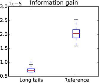
Figure 5: Boxplot of information gains (eq. (7)) obtained from fits to simulated data with Cauchy-distributed offspring (left) or Gaussian offspring (right). The poor fit from model misspecification is noticeable.

We performed several other simulations of different forms of misspecification, using boxcar and double exponential spatial distributions and also a Gamma distribution for offspring times. With spatial misspecification, the covariate coefficients were still unbiased on average, with slight biases in $\theta$ depending on the type of misspecification, and larger biases in $\omega$ (towards longer decay times). Misspecification of the offspring timing did not bias $\theta$, $\beta$, or $\omega$, but did cause systematic understimation of $\sigma^{2}$. These results suggest that the covariate coefficient estimates of the model are robust to misspecification of the self-excitation component, though the self-excitation parameters can be sensitive to misspecification, giving misleading estimates of cluster size and duration.

4.3 Unobserved covariates and confounding

Section 2 discussed the inherent confounding that can occur when estimating the effect of spatial covariates on crime without accounting for self-excitation. Fig. 1 demonstrated that this confounding is generic, occurring whenever there are covariates that affect crime over time. By building a self-exciting point process model that accounts for self-excitation and covariates, we can account for both and avoid the confounding.

We must, however, be aware of other types of confounding that can creep in. The most common is an unobserved covariate: there are many spatial factors that can influence crime rates, and it is unlikely we can directly measure all of them. Fig. 6 demonstrates the danger. A covariate may be causally related to another covariate as well as to crime rates, and if it is not observed and accounted for, the other covariate’s estimated effect will be confounded. This is directly analogous to the situation in ordinary regression, when unobserved predictors may confound regression coefficient estimates.

Figure 6: A simplified causal diagram depicting potential confounding: covariate 1 has a causal relationship with both covariate 2 and crime rates, and so if it is unobserved, estimates of covariate 2’s effect will be confounded.

On the other hand, if the two covariates are not correlated in any way, omitting one does not bias estimates of the other’s effect; in traditional regression its mean effect is simply added to the intercept and the individual effects simply add to the error variance. However, in the more complicated self-exciting point process model, omitted covariates may have other detrimental effects. Though Schoenberg (2016) suggests that parameter estimates remain asymptotically consistent when covariates are omitted, provided the effects of those covariates are sufficiently small, a series of simulations demonstrate the bias that appears in finite samples.

We generated covariates on a grid, drawing the covariate values from a Gaussian process with squared exponential covariance function to ensure there was some spatial structure. We first ran 100 simulations (each with new Gaussian process draws) of independent covariates, fitting a model with both covariates included and one with the second covariate omitted, each using the expectation maximization procedure described in Section 3.3. Simulations were performed with random true parameter values, and these values were recorded, along with the fits. It is apparent from the results that estimates of $\hat{\theta}$ are affected by the missing covariate: Fig. 7 shows the fits, as a function of the true value of $\beta_{2}$ used in the simulation, and a distinct pattern can be seen when the second covariate is omitted from the fit, with $\hat{\theta}$ having larger variance for larger values of $|\beta_{2}|$. On average, the estimated $\hat{\theta}$ with a missing covariate is larger than the true $\theta$ by $0.18$.

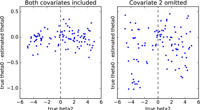
Figure 7: The difference between the true value of $\theta$ and the estimated value, as a function of the coefficient $\beta_{2}$, when the two covariates are independent. On the left, fits made when $\beta_{2}$ is accounted for; on the right, when it is not. Notice the odd behavior around $\beta_{2}=0$: when the omitted covariate does not matter, $\theta$ is estimated to be close to its true value, but when it has a larger effect, $\hat{\theta}$ has much higher variance.

Overestimation of $\theta$ has other consequences. For example, Fig. 8 shows a temporal residual plot (see Section 3.4) for a fit to a simulated dataset with an omitted covariate. An obvious calibration problem is present: by the time the 500th event occurred, the conditional intensity function predicted 150 fewer events than occurred. Near $t=0$, $\lambda(s,t)$ cannot predict the observed events because there is little past history of events; near $t=T$, a long past history and overestimated $\theta$ causes $\lambda(s,t)$ to overestimate the intensity and “catch up” in the cumulative predicted number of events.

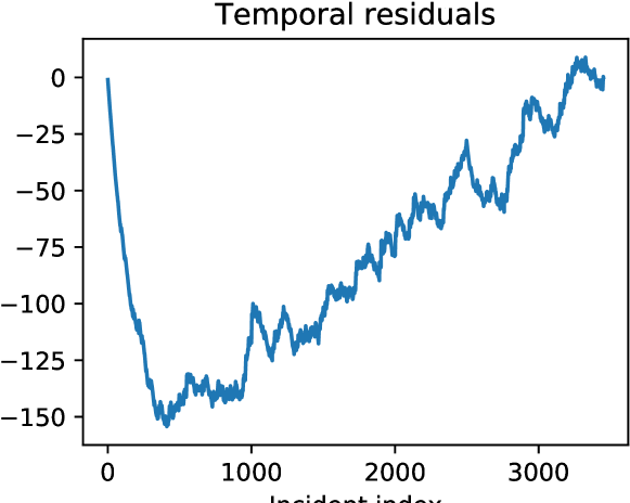
Figure 8: Temporal residual plot for a simulated fit with a missing covariate, demonstrating the effect of the overestimated $\theta$.

Additionally, the time decay parameter $\omega$ is also overestimated by 70% on average. Together, these biases suggest that the clustering induced by the unobserved covariate is being accounted for by increasing self-excitation and by allowing the effects of self-excitation to last longer in the model.

Next, we simulated causally confounded covariates, following the causal model in Fig. 6. Covariate 1 was drawn from a Gaussian process, as before, and Covariate 2 was defined to be the average of Covariate 1 and a separate independent Gaussian process. This gave an average correlation of $r=0.66$ between the covariates. Sample correlated covariates are shown in Fig. 9. Data was simulated from these covariates (with random coefficients) and then models fit with and without Covariate 2 included. Fig. 10 demonstrates the bias in estimates of $\beta_{1}$ that ensues when the effect of $\beta_{2}$ is not accounted for, similar to the biases that can occur in ordinary linear regression when covariates are confounded. The confounding also affects $\hat{\theta}$ and $\hat{\omega}$ in a similar way as in the previous simulation, with bias as $|\beta_{2}|$ increases.

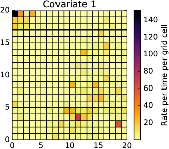
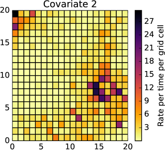
Figure 9: The rate induced (that is, $\exp(\beta X)$, where $\beta=1$ for simplicity and $X$ is the covariate) by two Gaussian process covariates on a $20\times 20$ grid. The second covariate is dependent upon the first. Notice the spatial structure of the Gaussian process.

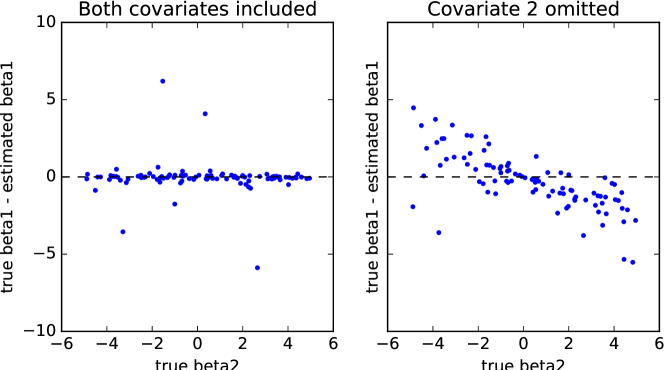
Figure 10: Bias observed in estimated values of $\beta_{1}$ when $\beta_{2}$ is also estimated (left) or is omitted from the fit (right).

Together, these simulations demonstrate two important caveats of self-exciting point process models:

1. Omitted spatial covariates, whether or not they are confounded with observed covariates, can bias estimates of the self-excitation parameter $\theta$, making it seem as though events are more likely to trigger offspring events.

2. Omitted spatial covariates can also bias estimates of the temporal decay parameter $\omega$, making it seem as though self-excitation or near-repeat effects occur over a longer timescale than they really do.

3. If there is a confounding relationship between covariates, such as that shown in Fig. 6, unobserved covariates can bias estimates of observed covariate effects ($\hat{\beta}$) as well as of self-excitation.

The first two points are particularly concerning, since in practical applications it is unlikely that all covariates could ever be accounted for—there will always be unmeasured spatial differences in base rates, or imperfectly measured covariates. This suggests that previous applications of self-exciting point process models may have overestimated the amount and time scale of self-excitation in the process, unless their background estimator was able to capture all spatial variation in base rates.

In some cases, the residual analyses introduced in Section 3.4 may make it possible to detect when there is an important unobserved spatial covariate. Temporal residual plots like Fig. 8 can suggest the presence of unobserved covariates (or other misspecification), while residual maps can make systematic deviations from the predicted event rate visible, and careful examination of the maps may suggest variables that need to be included. Section 5 gives examples of this in Pittsburgh crime data.

General approaches to account for unobserved covariates are more difficult. One strategy, sometimes used in spatial regressions, is to include a spatial random effect term intended to account for the unobserved covariates. However, at least in spatial regression, this method does not achieve its goal: a spatial random effect can bias coefficients of the observed covariates in arbitrary ways, particularly if the unobserved covariate is spatially correlated with any of the observed covariates (Hodges and Reich, 2010). Given the causal diagram in Fig. 1, it does not seem possible for any one adjustment to account for an unobserved covariate and give unbiased estimates of the effects of the other covariates. Users of spatial regression and the self-exciting point process model introduced here need to be aware of their limitations in the presence of unobserved confounders, and interpret results carefully.

5 Application

5.1 Pittsburgh incident data

To demonstrate the spatio-temporal model of crime proposed here, we will analyze a database of 205,485 police incident records filed by the Pittsburgh Bureau of Police (PBP) between June 1, 2011, and June 1, 2016, specifying the time and type of each incident and the city block on which it occurred. (Privacy regulations prevent PBP from releasing the exact addresses or coordinates of crimes, so PBP provides only the coordinates of the block containing the address.) The records include crimes from very minor incidents (such as 38 violations of Pittsburgh’s ordinance against spitting) to violent crimes, such as homicides and assaults. Only crimes reported to PBP are included, so the dataset does not include records from the police departments of Pittsburgh’s several major universities, including the University of Pittsburgh, Carnegie Mellon University, Chatham University, or Carlow University.

Because the database contains only incident reports, offense types are preliminary. Charges listed in the reports may be downgraded or dropped, suspects acquitted, or new charges filed. The reports represent only the charges reported by the initial investigating officers, so they may not correspond with final FBI Uniform Crime Report data or other sources. While this limits the accuracy of our data, it is also the only practical approach—final charges may not be known for months, so predictions based on them would be hopelessly out of date.

Rather than dealing with the numerous sections and subsections of the Pennsylvania Criminal Code represented in the incident data, we used the FBI Uniform Crime Report hierarchy, which splits incident types into a common hierarchy comparable across states and jurisdictions. Among so-called “part I” crimes, homicide, assault, and rape are at the top of the hierarchy, followed by other crimes like theft, burglary, and so on. If an incident involves two distinct types of crime (e.g. a burglary involving an assault on a homeowner), we use the type higher in the hierarchy, following the FBI’s “Hierarchy Rule” (FBI, 2004). The hierarchy of offenses is shown in Table 3. In our analysis we focused on crimes in these categories, though other “part II” crimes, such as simple assault and vandalism, are also available in the dataset, along with every other offense type recorded by the Pittsburgh Bureau of Police. Note that arson, typically hierarchy level 8, was miscoded in the data available to us, though arson was not used in any of our analyses.

Table 3: The part I crime hierarchy

Hierarchy	Crime	Count
1	Homicide	300
2	Forcible rape	893
3	Robbery	5884
4	Aggravated assault	5900
5	Burglary	11943
6	Larceny/theft	37487
7	Motor vehicle theft	3892
8	Arson	0

We also collected, from city and Census Bureau data, various spatial covariates for each Census block, including

• The fraction of residents who are male from age 18–24

• The fraction of residents who are black

• The fraction of homes that are occupied by their owners, rather than rented

• The total population

• Population density (per square meter)

• The fraction of residents who are black or Hispanic.

Some city blocks have no population (e.g. in commercial areas with no residents), so an additional dummy variable was used to record whether each block had a population. In all models that follow, population-based covariates only enter the models when the block has a nonzero population.

These covariates will be used to demonstrate the model’s ability to account for spatial factors that attract crime. They are not intended to be a comprehensive list of all possible risk factors, and undoubtedly there are other relevant covariates; systematic identification and evaluation of relevant spatial features is out of the scope of this work.

5.2 Burglary analysis

Selecting only the first year of burglary data, containing 2892 burglaries, we fit two models, one using only population density as a covariate and the other using additional covariates. The burglaries are mapped in Fig. 11, showing spatial structure in the locations of burglary hotspots across the city. The model fits are shown in Table 4 and Table 5. Asymptotically normal 95% confidence intervals based on Rathbun’s covariance estimator are also shown for each parameter. The additional covariates improve the model AIC from 179750 to 179319, an improvement of about 431 units. Notice the relative consistency of the self-excitation parameters $\hat{\omega}$ and $\hat{\sigma}^{2}$ between fits, and that, as expected from the discussion in Section 4.3, $\hat{\theta}$ decreases when additional covariates are added.

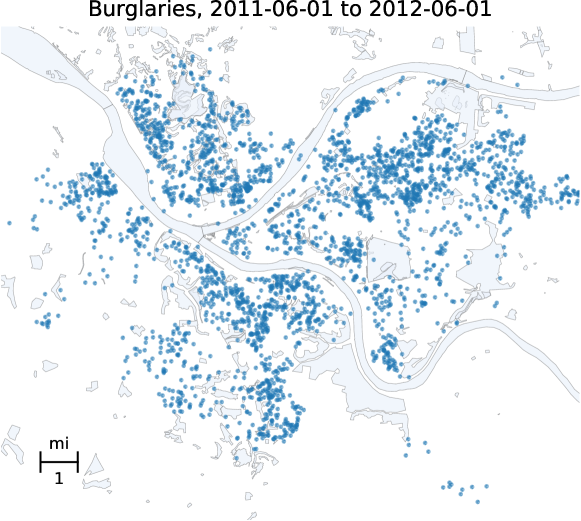
Figure 11: Locations of 2892 burglaries recorded in Pittsburgh between June 1, 2011 and June 1, 2012

Interpretation of the model with all covariates (Table 5) is straightforward. Each burglary stimulates or predicts, on average, $\hat{\theta}=0.59$ further burglaries, distributed with a spatial bandwidth of $\hat{\sigma}\approx 468$ feet at a rate exponentially decaying in time with parameter $\hat{\omega}\approx 47$ days. High population densities predict higher risks of burglary, as there are more residences to burgle; similarly, blocks with populations greater than zero (a proxy for residential vs. commercial blocks) have a higher burglary rate. The remaining covariates enter the model when blocks have a population greater than zero. Higher proportions of young men indicate a lower burglary risk, though the confidence interval for this effect overlaps zero. Home ownership, rather than renting, has a negative effect, while a higher fraction of black residents is correlated with higher burglary rates; these last two factors are likely confounded with poverty and socioeconomic status, which have strong relationships with crime but are not included in this model.

Table 4: Predicting burglary using population density

Parameter	Value	CI
$\theta$	0.764	[0.717, 0.811]
$\omega$	$4.511\times 10^{6}$ (52.21 days)	[47.04, 57.39]
$\sigma^{2}$	$2.664\times 10^{5}$ (516.1 feet)	[487.2, 543.5]
$\beta_{0}$ (intercept)	-31.63	[-31.50, -31.76]
$\beta_{1}$ (pop / $\text{m}^{2}$)	31.66	[8.91, 54.4]
AIC	179750

Table 5: Predicting burglary using additional covariates

Parameter	Value	CI
$\theta$	0.589	[0.544, 0.635]
$\omega$	$4.061\times 10^{6}$ (47.00 days)	[41.97, 52.04]
$\sigma^{2}$	$2.194\times 10^{5}$ (468.4 feet)	[439.0, 496.1]
$\beta_{0}$ (intercept)	-33.15	[-33.53, -32.78]
$\beta_{1}$ (pop / $\text{m}^{2}$)	25.50	[6.13, 44.86]
$\beta_{2}$ (block populated?)	2.49	[2.05, 2.92]
$\beta_{3}$ (frac. male 18–24)	-0.69	[-1.74, 0.36]
$\beta_{4}$ (frac. black)	0.75	[0.55, 0.95]
$\beta_{5}$ (frac. homes owned)	-1.14	[-1.40, -0.88]
AIC	179319

For a larger view of Pittsburgh, Fig. 12 shows an overall residual map of Pittsburgh over two months. Several trends appear, suggesting inadequacies in the available covariates and the presence of boundary effects: commercial areas such as downtown (at the confluence of the two rivers) have fewer burglaries than predicted, and the presence of the University of Pittsburgh and Carnegie Mellon University also results in negative residuals, as each has its own police department whose records are not included in our dataset. Note that, as discussed in Section 3.4, negative (blue) residuals visually dominate, because areas with lower-than-expected crime hence have larger Voronoi cells; also note the presence of several clusters of small cells with large positive residuals, at the locations of temporary burglary hotspots.

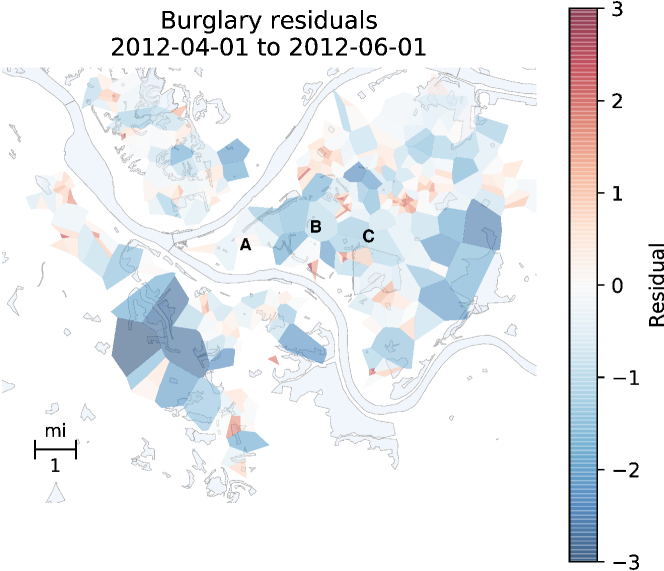
Figure 12: Residual map from the fit shown in Table 4, over two months of burglaries. A: downtown, B: University of Pittsburgh, C: Carnegie Mellon University.

To demonstrate leading indicators, we fit an additional model containing the same set of covariates but also two leading indicators, larceny/theft and motor vehicle theft (hierarchy levels 6 and 7). The fit is shown in Table 6, and shows that motor vehicle theft in particular seems predictive of burglary, with a coefficient of $\hat{\theta}_{2}=0.1167$. The AIC of this model further improved to 179201, by 118 units.

Table 6: Predicting burglary with leading indicators

Parameter	Value	CI
$\theta_{0}$ (self-excitation)	0.4480	[0.404, 0.492]
$\theta_{1}$ (larceny/theft)	0.0632	[0.049, 0.078]
$\theta_{2}$ (motor vehicle theft)	0.1167	[0.037, 0.197]
$\omega$	$3.551\times 10^{6}$ (41.10 days)	[36.5, 45.8] days
$\sigma^{2}$	$1.619\times 10^{5}$ (402.3 feet)	[376, 427] feet
$\beta_{0}$ (intercept)	-33.90	[-34.47, -33.33]
$\beta_{1}$ (pop / $\text{m}^{2}$)	25.19	[2.48, 47.9]
$\beta_{2}$ (block populated?)	3.00	[2.37, 3.63]
$\beta_{3}$ (frac. male 18–24)	-0.85	[-2.14, 0.43]
$\beta_{4}$ (frac. black)	0.94	[0.72, 1.15]
$\beta_{5}$ (frac. homes owned)	-1.00	[-1.30, -0.71]
AIC	179201

Temporal calibration plots for these models show patterns similar to Fig. 8, suggesting, as discussed in Section 4.3, that there is additional spatial heterogeneity in crime rates which is not accounted for by the available covariates in these models, and hence that the self-excitation parameters may be overestimates. Further research is necessary to identify relevant covariates and prepare higher-resolution covariate datasets to adequately model crime.

6 Conclusions

Self-exciting point processes have been used for a wide range of applications, from epidemiology to seismology, and we have built on this work to introduce an improved model for crime, extending previous crime models by incorporating spatial covariate information and providing parameter inference tools to aid understanding of the patterns of crime. Though self-exciting point process models are more complex than ordinary spatial regression, making analysis more difficult for users used to the wealth of tools available for regression, we have helped bridge this gap through interpretable residual diagnostic tools (adapted from related models) and through scoring methods for comparing the predictive performance of models, neither of which has previously been used with any crime hotspot analysis tool.

A contribution of our work is a demonstration, both theoretically and through simulations, that methods that focus purely on the spatial or temporal aspects of crime are generally confounded and can produce misleading results, requiring a method that accounts for both aspects simultaneously. This calls into doubt previous results on the connection of spatial features to crime, and the problem generalizes to self-exciting processes outside of crime, such as models of infectious disease and earthquakes. Extensive simulations characterize our model’s reaction to misspecification and omitted covariates, both likely problems to experience in real-world data.

Together, the tools and simulations presented in this paper provide a single comprehensive package of modeling, diagnostic, and inference tools for self-exciting point processes, which have not previously been assembled in one place. The model and tools will enable new criminological research, revealing patterns of crime, allowing tests of theories about the origin and dynamics of crime, and contributing to improved policing strategies. Additional research will more extensively explore the Pittsburgh crime dataset, along with other cities, and additional covariates and types of crime. Further, the tools and results described here apply beyond the analysis of crime, to any spatio-temporal process with self-excitation.

References

- Andresen et al. (2017) Andresen, M. A., Linning, S. J. and Malleson, N. (2017) Crime at Places and Spatial Concentrations: Exploring the Spatial Stability of Property Crime in Vancouver BC, 2003–2013. Journal of Quantitative Criminology, 33, 255–275.
- Baddeley et al. (2005) Baddeley, A., Turner, R., Møller, J. and Hazelton, M. (2005) Residual analysis for spatial point processes (with discussion). Journal of the Royal Statistical Society: Series B (Statistical Methodology), 67, 617–666.
- Bergstra et al. (2010) Bergstra, J., Breuleux, O., Bastien, F., Lamblin, P., Pascanu, R., Desjardins, G., Turian, J., Warde-Farley, D. and Bengio, Y. (2010) Theano: a CPU and GPU math expression compiler. In Proceedings of the Python for Scientific Computing Conference (SciPy).
- Bernasco et al. (2015) Bernasco, W., Johnson, S. D. and Ruiter, S. (2015) Learning where to offend: Effects of past on future burglary locations. Applied Geography, 60, 120–129.
- Braga et al. (2014) Braga, A. A., Papachristos, A. V. and Hureau, D. M. (2014) The Effects of Hot Spots Policing on Crime: An Updated Systematic Review and Meta-Analysis. Justice Quarterly, 31, 633–663.
- Brantingham and Brantingham (1981) Brantingham, P. J. and Brantingham, P. L. (1981) Environmental Criminology. SAGE Publications.
- Bray et al. (2014) Bray, A., Wong, K., Barr, C. D. and Schoenberg, F. P. (2014) Voronoi residual analysis of spatial point process models with applications to California earthquake forecasts. Annals of Applied Statistics, 8, 2247–2267.
- Cerdá et al. (2009) Cerdá, M., Tracy, M., Messner, S. F., Vlahov, D., Tardiff, K. and Galea, S. (2009) Misdemeanor policing, physical disorder, and gun-related homicide: a spatial analytic test of "broken-windows" theory. Epidemiology, 20, 533–541.
- Chainey et al. (2008) Chainey, S., Tompson, L. and Uhlig, S. (2008) The Utility of Hotspot Mapping for Predicting Spatial Patterns of Crime. Security Journal, 21, 4–28.
- Cohen et al. (2007) Cohen, J., Gorr, W. L. and Olligschlaeger, A. M. (2007) Leading Indicators and Spatial Interactions: A Crime-Forecasting Model for Proactive Police Deployment. Geographical Analysis, 39, 105–127.
- Cowling and Hall (1996) Cowling, A. and Hall, P. (1996) On pseudodata methods for removing boundary effects in kernel density estimation. Journal of the Royal Statistical Society Series B, 58, 551–563.
- Daley and Vere-Jones (2008) Daley, D. J. and Vere-Jones, D. (2008) An Introduction to the Theory of Point Processes, Volume II: General Theory and Structure, vol. 2. Springer, 2 edn.
- Daley and Vere-Jones (2004) Daley, D. T. and Vere-Jones, D. (2004) Scoring Probability Forecasts for Point Processes: The Entropy Score and Information Gain. Journal of Applied Probability, 41, 297–312.
- FBI (2004) FBI (2004) Uniform Crime Reporting Handbook. Department of Justice. URL: https://ucr.fbi.gov/additional-ucr-publications/ucr_handbook.pdf.
- Gneiting and Raftery (2007) Gneiting, T. and Raftery, A. E. (2007) Strictly Proper Scoring Rules, Prediction, and Estimation. Journal of the American Statistical Association, 102, 359–378.
- Gorr (2009) Gorr, W. L. (2009) Forecast accuracy measures for exception reporting using receiver operating characteristic curves. International Journal of Forecasting, 25, 48–61.
- Gorr and Lee (2015) Gorr, W. L. and Lee, Y. (2015) Early Warning System for Temporary Crime Hot Spots. Journal of Quantitative Criminology, 31, 25–47.
- Haberman and Ratcliffe (2012) Haberman, C. P. and Ratcliffe, J. H. (2012) The Predictive Policing Challenges of Near Repeat Armed Street Robberies. Policing, 6, 151–166.
- Harcourt and Ludwig (2006) Harcourt, B. E. and Ludwig, J. (2006) Broken Windows: New Evidence from New York City and a Five-City Social Experiment. The University of Chicago Law Review, 73, 271–320.